Evolution of network structure by temporal learning
Abstract
We study the effect of learning dynamics on network topology. A network of discrete dynamical systems is considered for this purpose and the coupling strengths are made to evolve according to a temporal learning rule that is based on the paradigm of spike-time-dependent plasticity. This incorporates necessary competition between different edges. The final network we obtain is robust and has a broad degree distribution.
1 Max Planck Institute for Mathematics in the Sciences, Inselstrasse
22, D-04103 Leipzig, Germany
2 Department of Physics, Ramniranjan Jhunjhunwala College, Ghatkopar (W), Mumbai 400 086, India
PACS codes: 89.75.Hc, 05.45.Ra, 87.18.Sn
Keywords: Coupled Maps, Scale-free Network, Hebbian Learning, Logistic Map, Synchronization.
∗Corresponding Author.
Email: jjost@mis.mpg.de Phone: +49-341-99 59 550 Fax: +49-341-99 59 555
1 Introduction
In recent years, several paradigms have been advanced for understanding the structural properties of networks in different domains, and certain rather universal features have been identified, like the small world property or a power law degree distribution, [1, 2]. In this context, also some principles for the generation of networks have been proposed that can be captured by slogans like “the rich get richer”[3, 2] or “make friends with the friends of your friends”[4]. We here pursue a somewhat different approach, namely the modification of an existing network by dynamical rules, but again with a view towards universal features. Our model originates from the observation of the temporal development of neuronal networks on the basis of the interplay between a fast activity dynamics at the neurons, the nodes in the network, and a slow learning dynamics affecting the strengths of the synapses, the edge weights of the network, see [5] as a general reference. Our aim here is to explore the possibility that some rather universal features of a learning process operating on and modifying a given edge can lead to robust network structures in the case of coupled chaotic oscillators. The neuronal networks in the brain consist of neurons connected to each other via directed synapses that transmit electrical signals between neurons. The potential of a neuron thus changes on a fast time scale depending on the inputs from other neurons. The strength of a synapse determines the efficiency of this synapse to transmit a signal. The dynamics of the strength of the synapses which is interpreted as learning is much slower than the dynamics of the neurons, see e.g. [6].
It is well-known that just after birth the brain has a very dense population of synaptic connection and, as time goes on, most of the connections are pruned (see, for example, [7]). This obviously happens as a result of learning. This leads to the question about the role of learning dynamics in deciding the final network structure.
2 Model
We wish to explore whether learning dynamics can lead to the pruning of a densely connected network and result in a robust sparsely connected network. We are not focussing on neurobiological details, but rather on general principles. In order that a dynamical network generate nontrivial behavior, we need some interplay of enhancing and reversing features, at the level of the dynamics of the individual elements or as a structural feature of the network connections. In typical neural network paradigms, the latter is achieved by the presence of both excitatory and inhibitory synapses, while the dynamics of an individual formal neuron could be defined by a monotonically increasing function of its inputs, e.g. by a sigmoid function. For suitable parameter regimes, the resulting collective network dynamics can be chaotic. The presence of inhibitory synapses, however, complicates the discussion of the learning rule; in particular, there is no good reason why the learning rules for excitatory and inhibitory synapses should be the same. As an alternative, one can consider a network with excitatory synapses only, but with a nonmonotonic dynamical function for the network elements. Simple such functions are the tent or logistic maps, which, for a suitable parameter choice, can lead to chaotic dynamics of the individual elements. Naturally, the collective network dynamics can then also be chaotic. Here, we choose the second option, with a logistic map for the individual dynamics. We are thus in the framework of coupled map lattices as introduced in [8]. In particular, such coupled map lattices can exhibit synchronized chaotic behavior, see [9] for a systematic analysis. This is helpful also for understanding some of the weight dynamics by our STDP rule below.
Our model thus abstracts from many properties of neurobiological networks, but we hope to thereby identify certain general aspects that should also be helpful for understanding the structure of networks as the result of structural changes from ongoing dynamical activity. We use a coupled map network and a simple learning rule arising from spike-time-dependent plasticity (STDP). The theoretical origin of that learning rule is the well known postulate of Hebb [10] that when an axon of a cell A is near enough to excite cell B or repeatedly or persistently takes part in firing it, some growth process or metabolic change takes place in one or both cells such that A’s efficiency, as one of the cells firing B, is increased.. On the basis of mathematical considerations[13, 14] and experimental findings[11, 12], a precise version says that the synaptic strength increases when the presynaptic neuron fires shortly before the postsynaptic one – in which case a causal contribution can be assumed –, but is weakened when that temporal order is reversed. (This mechanism is called spike-timing-dependent synaptic plasticity (STDP).) The latter feature, in an elegant manner, prevents the unbounded growth in synaptic strengths, a problem with earlier attempts to implement Hebb’s rule.
Such a mechanism would help to stabilize specific neuronal activity patterns in the brain. If neuronal activity patterns correspond to behavior, then the stabilization of specific patterns implies the learning of specific types of behaviors.
2.1 Coupled map network
As already mentioned, our model is not based on the dynamical features of real neurons that are described by Hodgkin-Huxley type equations, see e.g. [5]. We rather consider the following coupled dynamical system
| (1) |
where is an -dim column vector consisting of the state of the nodes of the network, is an coupling matrix that describes how the network is connected, and is a map from onto itself modeling the dynamics of the node. We consider chaotic dynamics, the logistic map defined as:
| (2) |
with . is the coupling strength of the edge from to , and we impose the balancing condition , as usual for coupled map lattices [8]. means that there is no link from to . We should note that we choose the for nonnegative, that is, we do not consider inhibitory synapses. Dynamically, this is compensated by the nonmonotonic behavior of (2). The key point is that we need to generate some nonmonotonic dynamics. This could be caused either by the interplay of excitation and inhibition in the transmission of activity between elements, as in most neural network models, or by a nonmonotonic dynamics of the elements themselves. We choose the latter option, because then the analysis of synchronization is easier.
The dynamics in equation (1) is discrete. The state vector at time instance gets updated by the nonlinear map and the coupling matrix to a new state vector at time instance . Also, the balancing condition mentioned above is imposed at every step.
2.2 The learning rule
In our model, the learning rule assigns a dynamics to the entries in the coupling matrix. For the above discrete dynamics, the learning rule also has to be discrete. We choose the following learning rule:
| (3) |
where is a small parameter deciding the time scale of
the learning dynamics. Thus, the strength of the connection from to grows when the state of at time and the state of at time are correlated, and it decreases when the correlation switches the temporal order, that is, when is active before .
This rule thus represents a discrete time implementation of STDP. When
two nodes are synchronized the coupling strength does not change. We
recall here that coupled map lattices synchronize under a wide range
of conditions, see [9], even though synchronization need not
and does not always occur in our simulations.
From a different perspective, in connection with information flows in networks, a general class of such learning rules has been considered in [15].
2.3 Networks
Our tools chosen for analyzing our networks are motif and eigenvalue distribution. Motif distribution refers to the distribution of small subnetworks and thus yields local information about the network. We consider only triads and count the number of occurences of different instances of connected subnetworks containing three sites. There are 13 different possible connected triads possible. In contrast, the eigenvalue distribution of the matrix yields global information about the network.
3 Results
In order to study the effect of learning on the network topology, we begin with a globally coupled network of discrete dynamical systems described in equations (1) and (2). The dynamics of the coupling strengths is governed by equation (3). We assign small nonzero initial values to the coupling strength and allow the system to evolve for about time steps depending on the number of nodes which we have taken as powers of 2, from 16 to 2048. Whenever the coupling strength of any edge becomes negative we clamp it to zero thereafter. This is pruning of the edge. We find that the evolution leads to a steady state with a robust heavy tailed network.
The initial values of strengths of the edges are distributed randomly (and uniformly) in an interval . The value of is chosen sufficiently small for two reasons. Firstly, we would like avoid initial near synchronization of any pair of nodes which, we observe, only slows the approach to the steady state. Secondly, since we start with a globally coupled network, every node gets an input from many other nodes during the initial phase of the evolution. If as a result of the addition of these inputs the value of the state variable exceeds unity then owing to the definition of the logistic map, it will grow without any limit during subsequent iterations. Therefore we choose . Obviously, the value of has to be smaller than . This severely restricts the choice of the parameter in our simulations. This choice of small initial values of the coupling strength is consistent with the biological example we have in mind. It is natural to expect that, just after birth, synapses will be weak and during the course of time some of them will strengthen and others will be pruned. In any case, only the ratio is relevant in deciding the time to reach the steady state.
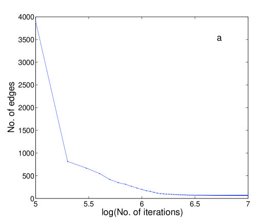
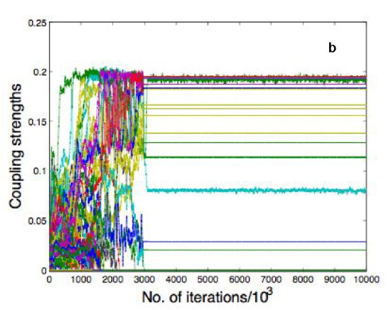
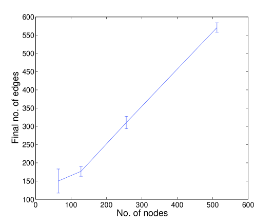
In Fig. 1a, the number of edges is plotted against the logarithm of the number of iterations. We see that the number of edges decreases very fast in the beginning and then reaches a constant value. Fig. 1b shows how individual edges evolve in a small system. The values of coupling strengths perform a random walk and few of them reach a positive value which is either constant or fluctuates around a constant mean value. The strengths of these remaining edges then are unlikely to become zero, preserving the structure of the final residual network intact. We checked this by allowing one realisation to run for iterations. We also added a small random noise with uniform distribution to the learning dynamics. This did not affect the conclusions. Thus it follows that as the system evolves the coupling strength of many edges drops to zero but at the same time some edges become stronger and their strength attains a steady value. This was found to occur for several values of the system size as well as different allowed values of . As depicted in Fig 2, we found that the number of edges in the final network is of the order of . The large error bar for a 64 node network could be a result of the large value of the ratio in this example.
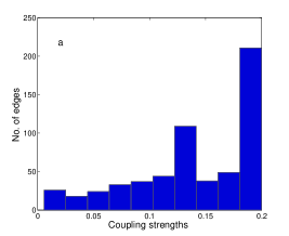
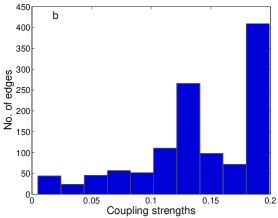
Next we look at the distribution of the coupling strengths in the final network. The Fig. 3 shows two examples. It is clear that the final distribution is the same and it is also consistent with the Fig. 1b which is for a small system.
Having established the existence of a robust network, we can study some of its properties and how robust they are. First we consider the frequency of different connected subnetworks of size three which yields local information about the network. Such a study is thought to be useful in uncovering the structural design principles of the network [16]. The network we obtain is rather sparse so we restrict ourselves only to motifs of size 3. Out of 13 possible only 4 motifs are present in the final network irrespective of the value of and the network size. If A, B and C are three different nodes then the four subnetworks are: (1) links going out from (say) B, (2) opposite of (1), i.e., links coming into B, (3) there is a link from A to B and a link from B to C and (4) a cyclic triangle. The other configurations are absent. In particular, triads with double links, i.e., a link from A to B and also from B to A, are absent. This is expected from the learning rule since is a constant and so, one of the link grows at the expense of the other. Noncyclic triangles are also absent.
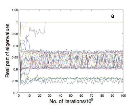
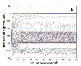
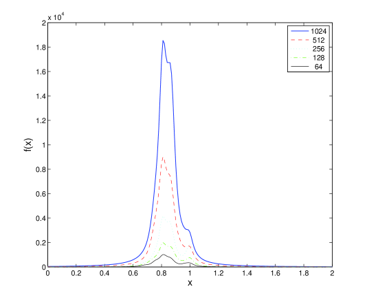
Now we study the eigenvalue distribution of the matrix which yields global information about the network. In Figs. 4a and b we plot the real part of the eigenvalues for a 32-node network and a 64-node network respectively. We see that the real part of a few eigenvalues becomes 1 corresponding to few nodes getting isolated. There is a lower bound which the real part of eigenvalues do not cross. This is a consequence of the existence of triangles. All other eigenvalues reach a steady value which is intermediate. In fact, they separate into bands which are robust. In order to succinctly show this for several system sizes we plot, in Fig. 5, the convolution of the real parts of the eigenvalues with Lorentz kernel as given by the function
| (4) |
where s are the real parts of the eigenvalues of the matrix and . The similar structure of the graphs over several system sizes is evident.
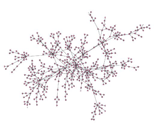
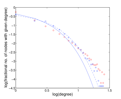
The most interesting outcome of this study is the final structure of the graph. We find that though some nodes and small clusters get separated there is still a single large connected component. In Fig. 6 we show the residual graph of 1024 nodes. The network has broad degree distribution. In Fig. 7, we show the degree distribution for 512 and 1024 node networks. We compare it with a geometric distribution with the same mean. The deviation from the exponential decay is clear.
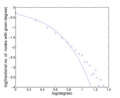
We have also started from a initial random network with degree 100 instead of the globally coupled network. This system reaches a steady state in less number of iterations and allows us to increase the size of the system. The degree distribution arising out of this simulations for 2048 node network is shown in Fig. 8 along with corresponding geometric distribution. This shows that the choice of initial network is not crucial for the final conclusion.
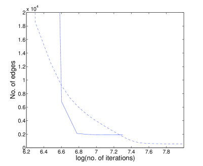
In all these simulations we have made sure that the system has reached a steady state by keeping track of the number of edges. Fig. 9 displays this fact.
Now we study the structure of the underlying network. That is, we consider the network disregarding the directions of the edges and study the eigenvalues of the Laplacian defined by
| (5) |
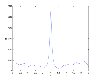
where is the state of site and is the number of neighbors of site . implies that and are neighbors. The spectrum of this operator yields important invariants of the underlying graph, see [17]. We again plot the spectral plot as in equation (4) of the eigenvalues of this operator in Fig 10. The structure of this plot is somewhat different from the ones obtained for other networks, see [18] for a systematic comparison with theoretical paradigms and empirical networks, even though the prominent peak near 1 is a feature exhibited by many empirical networks, see the diverse examples in [18].
4 Discussion
We have studied the effect of a STDP type learning rule on the network dynamics. This learning rule incorporated the necessary competition between different edges. As the network evolves, some edges grow in strength and some edges become weak and are then eliminated. This is much like the biological case wherein the brain is densely wired at the time of birth and then most synapses are pruned in the course of the development. In our setting, the resulting network is sparse and has broad degree distribution. The properties of the final network are universal in the sense that they do not depend on the system size and the value of within the allowed range. This suggests that there exists an attractor of the overall dynamics (nodes, synapses and network) to which the system evolves. This constitutes a mechanism to obtain heavy-tailed networks where no preferential attachment has been explicitly introduced. There exist some other works that obtain scale-free networks without overt preferential attachment, for example, [19, 20, 21]. The network we obtain is rather too sparse as compared to the real biological examples. The reason for this seems to be that our simple model only incorporates pruning due to learning dynamics. There are many processes, like exuberance, that can introduce new links. It remains to study the effects of such or other, biologically more realistic, dynamics and learning rules.
Note: After we had communicated this manuscript we became aware of the work by Shin and Kim [22] in which they have obtained similar results using the FitzHugh-Nagumo model.
Acknowledgement
KMK would like to acknowledge the financial assistance from DST (India). We should also thank the referees for their useful comments.
References
- [1] D. J. Watts and S. H. Strogatz, Nature (London) 393, 440 (1998).
- [2] A. L. Barabasi and R. A. Albert, Science 286, 509 (1999).
- [3] H.Simon, On a class of skew distribution functions, Biometrika 42, 425-440, 1955
- [4] J.Jost and Joy, Evolving networks with distance preferences, Phys.Rev.E 66, 36126-36132, 2002
- [5] P.Dayan and L.Abbott, Theoretical Neuroscience, MIT Press, 2001
- [6] G.Shepherd, Neurobiology, Oxford Univ.Press, 3rd ed., 1994
- [7] D. L. Bishop et al, Neuron 44, 651-661 (2004)
- [8] K. Kaneko. Period-doubling of kink-antikink patterns, quasi-periodicity in antiferro-like structures and spatial intermittency in coupled map lattices – toward a prelude to a field theory of chaos. Prog.Theor.Phys, 72:480–486, 1984.
- [9] J.Jost and Joy, Spectral properties and synchronization in coupled map lattices. Phys. Rev. E 65 (2002) 016201- 1–9
- [10] D.Hebb, The organization of behavior, Wiley, 1949
- [11] H.Markram, J.Lübke, M.Frotscher, B.Sakmann, Science 275, 213-215, 1997
- [12] L.Zhang et al, Nature 395, 37-44, 1998
- [13] R.Kempter, W.Gerstner, J.L.van Hemmen, Phys.Rev.E 59, 4498-4514, 1999
- [14] J.Jost, Theory Bioscienc. 125, 37–53, 2006
- [15] T.Wennekers, N.Ay, Neural Comp. 17, 2258–2290, 2005
- [16] R. Milo, et al, Science 298, 824-827, 2002
- [17] A.Banerjee, J.Jost, Discr.Appl.Math., in press
- [18] A.Banerjee and J.Jost, Spectral plot properties: Towards a qualitative classification of networks, Networks Heterogen.Media 3, 395-411, 2008
- [19] M. Baiesi and S. S. Manna, Phys. Rev. E 68, 047103 (2003)
- [20] H. Ebel and S. Bornholdt, arxiv.org/abs/cond-mat/0211666
- [21] T. Rohlf, arxiv.org/abs/0708.1637
- [22] C.-W. Shin and S. Kim, Phys. Rev. E 74, 045101(R) (2006)