Anisomagnetic quasi-achromats with small effective emittance

Abstract

Quasi-achromat lattices (small dispersion is allowed in their straight sections, between their cells) are considered; in a cell, there are bending magnets of two kinds, of unequal magnetic field. Minimization of the effective emittance is carried out by the following algorithm (which follows Teng, and partly Lee).

(1) Every inner dipole’s contribution to the natural emittance is minimized with respect to all optics parameters (relating to dispersion and beta-function), except for the shift parameter, $s_{0}$, which specifies the interval between the beta-function minimum and the center of a magnet; for a side bending magnet, its contribution to an integral relating to the effective emittance (the relation uses the fact that the arithmetic mean majorizes the geometric mean) is minimized. (2) The other parameters of dipoles (fields, lengths or angles ratios, shifts) are restricted with the boundary conditions: the equality of Courant-Snyder invariants on the exit from a magnet and on the entrance to the following one. (3) The minimum of effective emittance and the last free parameters (two or three) can be found by computation.

The accuracy of this method falls with decreasing of the number of internal dipoles in a cell, and still the isomagnetic Tanaka-Ando minimum (for the modified DBA$\!{}^{*}$-lattice which has no inner dipoles) is reproduced with accuracy better than half a percent. If the number of dipoles per cell does not exceed four, the smallest effective emittance (14% lower than TA-limit) is achieved for QBA$\!{}^{**}$-lattice where all dipoles have nonzero shifts.

1 Introduction

Growing requests and needs of users of synchrotron radiation call for further improvements of parameters of specialised synchrotron light sources. One of the most important parameters is the horizontal natural emittance, ${\epsilon}_{x}$ (it also defines, through some coupling, the vertical emittance). Its value depends on the magnetic structure (lattice) of a storage ring, and first of all – on parameters and arrangement of dipole magnets, which should provide a closed orbit for the electron beam. For achromatic lattices DBA (double bend achromat – two dipole magnets per cell), TBA, QBA, where the ‘intercell’ regions have zero dispersion, the conditions of natural emittance minimization are well known from the works of Teng, and Lee, [1, 2]. The emittance strongly decreases with increase of the number of dipole magnets in a ring,

$${\epsilon}_{x}\propto N^{-3}\,;$$

at that, the size and costs of storage ring grow with $N$ as well.

The figure of merit of an insertion device (ID), serving as a SR-source, is defined, however, by the effective emittance, which depends on dispersion (or Courant-Snider invariant) in the ID straight section. It turns out that the effective emittance can be lowered if to weaken the dispersion-free condition [3, 4]. Therefore, the beam optics of some electron rings (Elettra, ESRF), initially achromatic, of DBA kind, was modified (so called distributed dispersion lattice, or quasi-achromat, DBA*).

With the aim to further reduce the emittance in ESRF, together with the doubling of the number of dipoles, from 64 to 128, they are considering the possibility to use dipoles with varying (along the orbit) magnetic field [3, 5].

In this work the problem of minimization of the effective emittance is to be solved for the case when the lattice cell is symmetric (with respect to inversion in its center) and includes magnets of two types: internal dipoles $M_{0}$ and a pair of the end (or side) dipoles $M_{1}$; the total number of magnets in a cell is $m=m_{0}+2$. Modified lattices TBA* and DBA* correspond to $m_{0}=1$ and $m_{0}=0$, respectively. In the case $m_{0}=2$, the internal dipoles can also have non-zero shift; this case will be denoted as QBA**.

Dipoles with unequal fields serve as SR sources with different critical energy, i.e, with peak regions in different parts of X-ray spectrum, so they can serve better for different ‘classes’ of SR users. However, large number of free parameters, which describe anisomagnetic cell, makes the search of the best parameters (when the effective emittance is minimal) a very difficult problem.

Here a possible way, an algorithm to solve this problem is suggested, which divides the problem into a few more simple parts. In principle, this approach allows to consider more complex lattice, with three or even four kinds of dipole magnets.

2 Effective emittance

The horizontal emittance of electrons, ${\epsilon}_{x}$, and the effective (horizontal) emittance, ${\epsilon}_{\rm eff}$, are defined by the next expressions, relating to some integrals along the orbit (they depend on the orbit’s radius, $\rho$, and optics function, including $\beta$-function) [2, 3, 4]:

$${\epsilon}_{x}=C_{q}\,\gamma^{2}\,\varepsilon_{x},\ \varepsilon_{x}=\frac{I_{5}}{J_{x}I_{2}}=\frac{I_{5}}{I_{2}-I_{4}},$$ (1)

$${\epsilon}_{\rm eff}=C_{q}\,\gamma^{2}\,\varepsilon_{\rm eff}\,,\ \varepsilon^{2}_{\rm eff}=\varepsilon_{x}\left(\varepsilon_{x}+\frac{H_{\rm ID}\,I_{3}}{2I_{2}+I_{4}}\right).$$ (2)

Here $\gamma$ is relativistic factor,

$$C_{q}=3.84\times 10^{-13}\,\mbox{m},\ \,C_{q}\gamma^{2}=1470\,{\rm nm}\,(E[{\rm GeV}])^{2};$$

these are the usual notations of some ring integrals:

$$\begin{array}[]{l}I_{2}=\oint\rho^{-2}\,ds,\ \ I_{4}=\oint\eta\rho^{-3}(1+2k\rho^{2})\,ds,\\ I_{3}=\oint|\rho|^{-3}\,ds\,,\ I_{5}=\oint|\rho|^{-3}H\,ds\,;\end{array}$$ (3)

$H_{\rm ID}$ in (2) is the Courant–Snyder invariant in the region of insertion devise,

$$H=\beta^{-1}\{\eta^{2}+(\alpha\eta+\beta\eta^{\prime})^{2}\},$$ (4)

$\alpha=-\frac{1}{2}\beta^{\prime}$; $\eta$ is dispersion function.

Some rings, sources of SR, were designed that the regions of ID would have invariant $H_{\rm ID}$ vanishing (i.e., dispersion and its derivative are both zero), but in the curse of time, lattice parameters were changed to reach better minimization of the effective emittance (2).

Integral $I_{4}$ is small in comparison with $I_{2}$, so it can be neglected, in the case of separate function magnets (dipoles have no quadrupole component, and $k=0$).

So, we seek to minimize the next combination of ring integral:

$$\varepsilon^{2}_{\rm eff}=\frac{I_{5}I_{6}}{I_{2}^{2}}=\frac{I_{5}(I_{5}+H_{\rm ID}\,I_{3}/2)}{I_{2}^{2}}\,;$$ (5)

and here one should note that integrals $I_{2}$ and $I_{3}$ depends only on the field of dipoles (radius of the orbit), but does not depend on betatron and dispersion functions. On the other hand, integrals $I_{5}$ and $I_{6}=I_{5}+H_{\rm ID}\,I_{3}/2$ are a sum of positive contributions from all magnets (because the Courant-Snyder invariant is always positive).

Therefore this problem of optimization can be attempted to be divided into a few relatively simple steps, that is, to be factorized:

(1) Firstly, we make minimization of a magnet’s contribution to $I_{5}$ with respect to parameters $\beta_{0},\,\eta_{0},\,\eta^{\prime}_{0}$, i.e., the value of beta-function at its minimum, and the dispersion functions in the point of this minimum (this point serves as the reference point, zero point of the orbit coordinate $s$ in a dipole); for the end magnets, which neighbour ID straight sections and directly define invariant $H_{\rm ID}$, we minimize their contribution to the sum $I_{5}+I_{6}$, because it approximates in a good way the necessary minimization of the product $I_{5}I_{6}$ (the arithmetic mean majorizes the geometric mean).

(2) The other dipole’s parameters – the curvature $\rho^{-1}$ (or the field), the length or the angle of rotation, $l=\vartheta\rho$, as well as the the coordinate of dipole’s center, $s_{0}$, or the (dimensionless parameter) shift, $x=-2s_{0}/l$, – should be restricted with the matching condition, which states the equality of the Courant–Snyder invariants on the exit from a dipole and on the entrance to the next one. One more restriction is that the orbit is closed, i.e., the sum of angles $\vartheta_{i}$ of all dipole magnets is equal to $2\pi$.

(3) After eliminating the angles, one can minimize the effective emittance with respect to the rest (two or three) parameters:

$$\kappa=\rho_{1}/\rho_{0},\ x=x_{0},\ y=x_{1}$$

(the internal magnets can have nonzero shift $x_{0}$, if their number is two).

It is well known that the contribution of a dipole magnet to the (natural) emittance is minimal when its center coincide with the minimum of beta-function (besides, this minimum and the dispersion parameters should have definite values depending on the magnet’s field [1, 2]). Such a magnet can be called symmetric (of symmetric arrangement), or unshifted; otherwise, we have a magnet with a shift.

As a rule, lattices consist of repeating, equal collections of dipole magnets – cells or periods (or superperiods). We will consider quite general case of a periodic lattice of $n$ symmetric cells (inversion in the cell center). Every cell contains $m$ dipole magnets, including $m_{0}=m-2$ internal magnets $M_{0}$ (unshifted, as a rule), and two (one on each side) end magnets $M_{1}$, with a shift $x_{1}$. Considering the right half of the cell, we will imply that the shift of the end magnet is positive (and it is negative in the left half of the cell). The total number of dipoles is $N=n\cdot m$; their rotation angles, $\vartheta_{0},\,\vartheta_{1}$, should comply with the requirement:

$$\sum\vartheta_{i}=n(m_{0}\vartheta_{0}+2\vartheta_{1})=2\pi\,.$$ (6)

Let us introduce the notation of the mean angle: $\bar{\vartheta}=2\pi/N$.

3 Minimization of contribution (to the emittance) of the internal dipoles

Let the length of a magnet is $l=\rho\vartheta$, and the coordinate of its center (from the minimum of beta-function) is $s_{0}=-xl/2$.

Following Teng [1], one can write the contribution of a magnet to integral $I_{5}$, as well as the Courant–Snyder invariant at its right and left edges, $H_{\pm}$, in the next form (see the expression (9)–(11) from [1]):

$$H_{\!\pm}=\beta_{0}(\eta^{\prime}_{0}+\sin\varphi_{\!\pm})^{2}+\frac{\rho^{2}}{\beta_{0}}\left(\!1-\frac{\eta_{0}}{\rho}-\cos\varphi_{\!\pm}\!\right)^{\!2}\!\!,$$ (7)

$$\Delta I_{5} \equiv \frac{1}{\rho^{3}}\int_{s_{-}}^{s_{+}}\!H\,ds=\frac{\vartheta\beta_{0}}{\rho^{2}}[A+D+(\eta^{\prime}_{0}+E\sin\varphi_{0})^{2}]$$ (8)

$$+ \frac{\vartheta}{\beta_{0}}[A-D+(1-\frac{\eta_{0}}{\rho}-E\cos\varphi_{0})^{2}],$$

$$\mbox{where }s_{\pm}=s_{0}\pm\frac{l}{2},\ \varphi_{\pm}=\frac{s_{\pm}}{\rho},\ \varphi_{0}=\frac{s_{0}}{\rho}=-\frac{x\vartheta}{2},$$

$$\!\left\{\!\!\begin{array}[]{l}A=\frac{1}{2}-\frac{1-\cos\vartheta}{\vartheta^{2}}\approx\frac{\vartheta^{2}}{4!}-\frac{\vartheta^{4}}{6!},\\[5.0pt] B=\frac{1}{2}-A-\frac{\sin\vartheta}{2\vartheta}\approx\frac{\vartheta^{2}}{4!}-\frac{2\vartheta^{4}}{6!},\\[5.0pt] D=B\cos 2\varphi_{0}\approx\frac{\vartheta^{2}}{24}\left[1-\frac{\vartheta^{2}}{30}(2+15x^{2})\right],\\[5.0pt] E=\frac{\sin(\vartheta/2)}{\vartheta/2}\approx 1-\frac{\vartheta^{2}}{24}+\frac{\vartheta^{4}}{16\cdot 5!}.\end{array}\right.$$ (13)

The last term in the last equation is added to show how quickly decreases the contribution of the further series terms. It is assumed that angles $\vartheta_{i}$ are small enough (for all dipoles of the storage ring), so already the first terms of angle expansion gives a sufficient accuracy.

Minimization of expression (8) with respect to $\eta_{0},\,\eta^{\prime}_{0}$ is reached if these parameters complies with the next conditions [1]:

$$\left\{\begin{array}[]{l}\eta^{\prime}_{0}=-E\sin\varphi_{0}\approx\frac{\,x\vartheta}{2},\\[5.0pt] \eta_{0}=\rho-\rho E\cos\varphi_{0}\approx\rho\vartheta^{2}\frac{1+3x^{2}}{24}\,.\end{array}\right.$$ (14)

The dipole’s contribution to the integral takes the form

$$\Delta I_{5}=\frac{\vartheta}{\rho}\left\{\frac{\beta_{0}}{\rho}(A+D)+\frac{\rho}{\beta_{0}}(A-D)\right\}\,;$$

further minimization with respect to $\beta_{0}$ gives now

$$\beta_{0}^{2} = \rho^{2}\frac{A-D}{A+D}\approx\rho^{2}\vartheta^{2}\frac{1+15x^{2}}{60},$$ (15)

$$\Delta I^{\rm(min)}_{5} = \frac{2\vartheta}{\rho}\sqrt{A^{2}-D^{2}}\approx\frac{\vartheta^{4}\sqrt{1+15x^{2}}}{12\sqrt{15}\rho}.$$ (16)

Taking into account (14), (15), one can reduce equation (7) to the following one:

$$H_{\pm}\approx\rho\vartheta^{3}\frac{4\mp 15x+45x^{2}}{12\sqrt{15}\sqrt{1+15x^{2}}}\,.$$ (17)

At $x=0$, we obtain the expressions for the central (unshifted) magnet (the case A of Teng). A lattice composed of $N$ such magnets (let $\rho=1$, then $I_{2}=I_{3}=N\vartheta,\ I_{5}=N\Delta I_{5}$), corresponds to the case of minimal natural emittance,

$$\varepsilon_{0}=\frac{\bar{\vartheta}^{\,3}}{12\sqrt{15}}\,\left(=\frac{I_{5}}{I_{2}}\right);\ \ \bar{\vartheta}=\frac{2\pi}{N}\,(=\vartheta);$$ (18)

the effective emittance of this lattice is equal to $3\varepsilon_{0}$.

It is convenient to measure emittances in units of $\varepsilon_{0}$, through introduction of dimensionless values $f,\,g$. It is known [2], that for the DBA lattice

$$f\equiv\frac{\varepsilon_{x}}{\varepsilon_{0}}=3,\ \ g\equiv\frac{\varepsilon_{\rm eff}}{\varepsilon_{0}}=3.$$

Dipoles of DBA-lattice have the shift $x=\frac{1}{4}$; using this value $x=\frac{1}{4}$ in (14)–(17), one can obtain (the effective emittance of such a quasi-achromat lattice is smaller in comparison with DBA case) $f=\frac{\sqrt{31}}{4},\ g=\frac{111}{8\sqrt{31}}\approx 2.49.$ At the point of minimum of $H_{+}(x)$, see (17), $x=0.229$ (this is the root of equation $45x^{3}+2x=1$), the effective emittance becomes yet some smaller: $g=2.43$. However, the more exact approach to minimize DBA* is to use another way to choose the optics parameters – as for the end dipoles.

4 Minimization of the end dipoles’ contribution to the effective emittance

Let the integral over all cell dipoles but the end ones is equal to $I^{*}_{5}$, and the end dipole’s contribution is $\Delta I_{5}$. Accounting for equation (5), we have

$$\Delta(I_{5}I_{6}) = n^{2}(I^{*}_{5}+2\Delta I_{5})(I^{*}_{5}+2\Delta I_{6})-n^{2}(I^{*}_{5})^{2}$$

$$\approx 2n^{2}I^{*}_{5}(\Delta I_{5}+\Delta I_{6})\propto 2\Delta I_{5}+JH_{+}/2\,.$$

Here $J=I_{3}/(2n)$ – integral along the half-cell, $n$ is the number of cells. Using (7)–(13), one can find the expression, which should be minimized (with respect to dipole’s parameters $\eta_{0},\eta^{\prime}_{0},\beta_{0}$; for simplicity sake, take for a while $\rho=1$):

$$\Delta I_{5} + \Delta I_{6}=2\vartheta\beta_{0}[A+D+(\eta^{\prime}_{0}+E\sin\varphi_{0})^{2}]$$

$$+\frac{2\vartheta}{\beta_{0}}[A-D+(1-\eta_{0}-E\cos\varphi_{0})^{2}]$$

$$+ \frac{J\beta_{0}}{2}(\eta^{\prime}_{0}+\sin\varphi_{\!+})^{2}+\frac{J}{2\beta_{0}}(1-\eta_{0}-\cos\varphi_{\!+})^{2}.$$

Zeroing the derivatives by $\eta^{\prime}_{0}$ and $\eta_{0}$, one can find the values of these parameters when the minimum occurs (restore $\rho$):

$$\left\{\begin{array}[]{l}\eta^{\prime}_{0}\approx\frac{\,\vartheta}{2}\cdot\frac{4y\vartheta-J\rho^{2}(1-y)}{4\vartheta+J\rho^{2}}\,,\\[5.0pt] \eta_{0}\approx\frac{\rho\vartheta^{2}}{24}\cdot\frac{4\vartheta(1+3y^{2})+3J\rho^{2}(1-y)^{2}}{4\vartheta+J\rho^{2}}\,;\end{array}\right.$$ (20)

here $y$ is the shift of end dipoles. Substituting this values to (4) one can obtain:

$$\Delta I_{5} + \Delta I_{6}=\frac{\vartheta^{3}}{6}\left\{4\beta_{0}\frac{\vartheta+J}{4\vartheta+J}\right.$$ (21)

$$+ \left.\frac{\vartheta^{2}}{60\beta_{0}}\left[1+15y^{2}+\frac{5J(1-3y)^{2}}{4\vartheta+J}\right]\right\}\,;$$

the minimum is reached if (restore $\rho$)

$$\beta^{2}_{0}=\rho^{2}\vartheta^{2}\frac{2\vartheta(1{+}15y^{2})+3J\rho^{2}(1{-}5y{+}10y^{2})}{120(\vartheta+J\rho^{2})}\,.$$ (22)

The edge CS-invariant takes the form:

$$H_{\pm} = \frac{\beta_{0}\vartheta^{2}}{4}\left[\frac{4\vartheta+J\mp J}{4\vartheta+J}\right]^{2}$$ (23)

$$+ \frac{\vartheta^{4}}{9\beta_{0}}\left[\frac{\vartheta\mp 3y\vartheta+(3\mp 3)yJ/4}{4\vartheta+J}\right]^{2}\,.$$

In principle, now all is ready for the final minimization: in addition to equations (21)–(23) one has to take into account that $\Delta I_{6}-\Delta I_{5}=JH_{+}/2\,.$

5 Minimization for DBA*-lattice

In order to check the appropriateness of the equations of the previous section, let us consider the simplest quasi-achromat lattice, with two magnets in a cell. In this case (in this section again $\rho=1$)

$$J\equiv I_{3}/N=\vartheta=\bar{\vartheta},$$

and equations (20)–(23) lead to

$$\left\{\begin{array}[]{l}\eta^{\prime}_{0}=\vartheta\frac{5y-1}{10}\,,\ \,\eta_{0}=\vartheta^{2}\frac{7-6y+15y^{2}}{120}\,,\\[5.0pt] \beta_{0}=\frac{\vartheta\sqrt{1-3y+12y^{2}}}{4\sqrt{3}}\,.\end{array}\right.$$

$$\Delta I_{5} + \Delta I_{6}=2\vartheta^{4}\frac{\sqrt{1-3y+12y^{2}}}{15\sqrt{3}},$$

$$H_{+} = \vartheta^{3}\frac{7-33y+72y^{2}}{75\sqrt{3}\sqrt{1-3y+12y^{2}}}.$$

As a result, we find the expressions for the ‘simple’ dimensionless emittances (natural and effective, respectively), see (18):

$$\begin{array}[]{l}f=\frac{\Delta I_{5}}{\vartheta\varepsilon_{0}}=\frac{13-27y+168y^{2}}{5\sqrt{5{-}15y{+}60y^{2}}}\,,\ g^{2}{=}\frac{\Delta I_{5}\Delta I_{6}}{\vartheta^{2}\varepsilon^{2}_{0}},\\[7.0pt] g^{2}=\frac{3(13-27y+168y^{2})(9-31y+104y^{2})}{125(1-3y+12y^{2})}\,.\end{array}$$ (24)

Figure 1: ‘Simple’ emittances of DBA* quasi-achromat lattice: $f$ – natural, $g$ – effective.

The corresponding curves are shown at the fig. 1. The minimum of effective emittance if reached at $y=0.107$, and its value is $g_{\rm min}=1.559$. So, the suggested minimization algorithm reproduces with an accuracy better than half a percent the minimum of Tanaka–Ando [4], which is 1.552.

It the next section we will consider more complex lattices, when the cell includes internal dipoles, with zero shift.

6 Lattices TBA*, QBA*, et cet.

Let $m_{0}$ is the number of internal dipoles, and $m=m_{0}+2$ is the total number of dipoles in a cell. We introduce the next dimensionless parameters:

$$q=\vartheta_{1}/\bar{\vartheta},\ p=\vartheta_{0}/\vartheta_{1},\ \kappa=\rho_{1}/\rho_{0},$$

and let $\rho_{1}=1$ (unit length). We will also omit in equations the mean angle (i.e., taking formally $\bar{\vartheta}=1$), because it should not enter into the simple emittance, both $f$ and $g$.

Still it is impossible to find $g(y,\kappa;\,m_{0})$ in an explicit form, but one can find this function through a numerical computing, according the following algorithm.

The orbit’s closure condition and the first integrals along the half-cell, normalized on $\vartheta_{1}$, see (3), read:

$$q=\frac{m}{m_{0}p+2}\,,\ \ i_{2}\equiv I_{2}/(2n\vartheta_{1})=1+\frac{m_{0}}{2}p\kappa\,,$$

$$j\equiv J/\vartheta_{1}=I_{3}/(2n\vartheta_{1})=1+\frac{m_{0}}{2}p\kappa^{2}\,.$$ (25)

Equation (22) gives (after normalization)

$$b\equiv\frac{\beta^{(1)}_{0}}{\vartheta_{1}}=\sqrt{\frac{2+30y^{2}+3j(1-5y+10y^{2})}{120(1+j)}}\,.$$

In the same way (23) and (21) transform to

$$h_{\pm}\equiv\frac{H^{(1)}_{\pm}}{\vartheta^{3}_{1}},\ \,S\equiv\frac{\Delta I^{(1)}_{5}+\Delta I^{(1)}_{6}}{\vartheta_{1}^{4}}=\frac{4b(1+j)}{3(4+j)}\,.$$

The matching condition $H_{+}^{(0)}=H_{-}^{(1)}$ gives

$$\frac{p^{3}}{3\sqrt{15}\kappa}=b\frac{(2+j)^{2}}{(4+j)^{2}}+\frac{(2+6y+3jy)^{2}}{36b(4+j)^{2}}\,(=h_{-}).$$ (26)

Equation (26) subject to (25) can be solved numerically; this gives a unique solution $p(y,\kappa;\,m_{0})$. Now, one can find $b(y,\kappa;\,m_{0})$ (i.e., the minimum of beta-function of the end dipole, $\beta^{(1)}_{0}$), and, at last, calculate $f$ and $g$:

$$i_{5}=\frac{I_{5}}{2n\vartheta_{1}}=\frac{q^{3}}{4}(2m_{0}\varepsilon_{0}p^{4}\kappa+2s-jh_{+}),$$ (27)

$$f=\frac{i_{5}}{\varepsilon_{0}i_{2}}\,,\ \,g^{2}=f\!\left(\!f+\frac{q^{3}jh_{+}}{2i_{2}\varepsilon_{0}}\!\right);\ \varepsilon_{0}{=}\frac{1}{12\sqrt{15}}\,.$$ (28)

Fig. 2 shows the region of the effective emittance minimum, $g(y,\kappa)$, for TBA* lattice. The Table contains parameters, including the natural emittance, for quasi-achromat lattices mBA* up to $m=10$.

Table 1: Parameters of quasi-achromats mBA*

$m$	2	3	4	5	6	7	8	9	10
$g_{\rm min}$	1.559	1.435	1.353	1.297	1.257	1.226	1.202	1.182	1.166
$f$	1.191	1.207	1.196	1.182	1.169	1.156	1.146	1.136	1.128
$y$	0.107	0.157	0.185	0.203	0.215	0.224	0.231	0.236	0.240
$\kappa$	–	0.850	0.835	0.830	0.831	0.832	0.835	0.839	0.843
$p$	–	1.134	1.170	1.198	1.222	1.241	1.258	1.272	1.285

Figure 2: Effective emittance $g(\kappa,y)$ for TBA$\!{}^{*}\!$ lattice.

7 Lattice QBA**

If $m=4$, i.e., four dipoles in a cell, the internal dipoles can also have a non-zero shift, $x_{0}=x$ (the shift of side dipoles is $x_{1}=y$). This time, one should change the left hand side of equation (26) using equation (17):

$$\frac{p^{3}(4-15x+45x^{2})}{12\kappa\sqrt{15}\sqrt{1+15x^{2}}}=h_{-}(j,y).$$

Moreover, in eq-n (27) for $i_{5}$, the contribution of internal dipoles should be changed [see(16)]:

$$i_{5}=\frac{q^{3}}{4}(2m_{0}\varepsilon_{0}p^{4}\kappa\sqrt{1+15x^{2}}+2s-jh_{+}).$$

Now we need to find a minimum of the function of three variables, $g(y,x,\kappa)$. One can consider two-dimensional sections, for different values of $\kappa$, seeking for the minimum $g_{\rm min}(\kappa)$; the plot of this function is shown on the fig. 3.

Fig. 4 shows the region of $g$-minimum for the case $\kappa=0.74$ (one can compare with the fig. 2). The minimum itself, $g_{\rm min}=1.345$, is reached at $y=0.181,\ x=0.046$ (at that $p=1.184$).

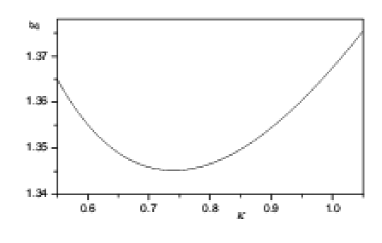
Figure 3: Lattice QBA**: emittance $g_{\rm min}$ vs. $\kappa=\rho_{1}/\rho_{0}$.

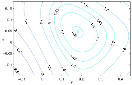
Figure 4: QBA$\!{}^{**}$: $g(y,x)$ near its minimum; at $\kappa=0.74$.

8 Conclusion

Anisomagnetic lattices with two sorts of magnets, TBA*, QBA*, and especially QBA** (internal magnets are shifted too) can have a bit smaller effective emittance, below the Tanaka–Ando minimum $g_{\rm TA}=1.552$; in the case of QBA** – up to $g_{\rm min}=1.345$. It is interesting that the new minimum is reached when the field of the internal magnets is smaller, at the level 74%, than that of the side magnets (so, one can consider the variants when internal magnets have quadrupole and/or sextupole component). One can consider more complex lattices, with tree kinds of magnets; note that the matching condition between internal dipoles is much simpler than between internal and end magnets.

The region of minimum is of clear advantages, like the better stability with respect to different tolerances, misplacement and misalignment errors, and so on, – because all gradients are small there.

The suggested minimization algorithm is heuristic in a sense; perhaps, it could be a bit complicated. For the end magnets, instead of the sum $2\Delta I_{5}+H_{+}J/2$, one can minimize a general linear combination $2\Delta I_{5}+\lambda H_{+}J$; the additional parameter $\lambda\approx 0.5$ should be chosen to lower the minimum $g_{\rm min}$.

I express my thanks to K. V. Zolotarev, who has attracted my attention to this problem, for interest to this work and a number of useful remarks.