An Analysis of Node-Based Cluster Summation Rules in the Quasicontinuum Method

Abstract.

We investigate two examples of node-based cluster summation rules that have been proposed for the quasicontinuum method: a force-based approach (Knap & Ortiz, J. Mech. Phys. Solids 49, 2001), and an energy-based approach which is a generalization of the non-local quasicontinuum method (Eidel & Stukowski, J. Mech. Phys. Solids, to appear). We show that, even for the case of nearest neighbour interaction in a one-dimensional periodic chain, both of these approaches create large errors when used with graded and, more generally, non-smooth meshes. These errors cannot be removed by increasing the cluster size. We offer some suggestions how the accuracy of (cluster) summation rules may be improved.

1. Introduction

The quasicontinuum (QC) method [16, 15, 18, 19] is a prototypical coarse-graining technique for the static and quasi-static simulation of crystalline solids. One of its key features is that, instead of coupling an atomistic model to a continuum model, it uses the atomistic model also in the continuum region where degrees of freedom are removed from the model by means of piecewise linear interpolation.

However, the nonlocal nature of the atomistic interactions makes further approximation necessary to enable the computation of energies or forces with complexity proportional to the number of coarse degrees of freedom. Two families of approximations have been developed to achieve this goal. One family of approximations localizes the interactions by a strain energy density (based on the Cauchy–Born rule) which provides sufficient accuracy in regions away from defects where the strain gradient varies slowly. Classical finite element methodology can then be utilized in those regions modeled by the strain energy density. This class of quasicontinuum approximations have been the subject of many recent mathematical analyses  [5, 12, 13, 6, 4, 2, 3, 7, 17].

The purpose of the present paper is to investigate the second family of approximations that have been developed to reduce the computational complexity of the quasicontinuum method. These methods, which have received far less mathematical attention, use summation rules (discrete variants of continuous quadrature rules) to approximate the sums that define the quasicontinuum energy or forces. To the best of our knowledge, the force-based cluster summation rule of Knap and Ortiz [11], the non-local QC method based on a simple trapezoidal rule [15, Sec. 3.3], or its extension to energy-based cluster summation rules [8] have not been analyzed to date. These cluster summation rules approximate the sum over atom-based quantities by uniformly averaging over atoms in clusters (balls) around the nodes and then by weighting these cluster averages so that summands that are obtained from piecewise linear interpolation with respect to the quasicontinuum mesh are exactly computed.

In a recent benchmark of different QC methods [14], the cluster summation rules do not compare favorably with quasicontinuum approximations that utilize the strain energy density or with other atomistic-to-continuum coupling methods. In the present paper, we give a simple yet rigorous analytical explanation for this poor performance. We demonstrate that, even for the simplest imaginable atomistic model, a periodic one-dimensional chain with harmonic nearest-neighbour interaction, the cluster summation rules formulated in [11, 8] lead to inconsistent and inaccurate QC methods when used with graded and non-smooth meshes. Increasing the cluster size does not resolve this problem. The benchmark [14] uses a mesh that is refined from large triangles to the atomistic scale as is typical for quasicontinuum computations. Our analysis shows that this kind of refined mesh would lead to an inconsistent and inaccurate method for the approximation of our one-dimensional model by cluster summation rules.

The atomistic model, the finite element space (coarse space), and some additional notation are introduced in Sections 1.1 and 1.2. We treat the two classes of cluster summation methods separately; the force-based summation rule in Section 2 and the energy-based summation rule in Section 3. These sections can be read independently of each other. Finally, in the conclusion, several possibilities are identified how cluster summation rules might be modified in order to lead to accuracte QC methods.

Although our analysis treats the approximation of the discrete sums in the quasicontinuum energy, the reasons for the lack of accuracy of the cluster summation rules can already be understood from applying the cluster-method concepts to the finite element approximation of continuum elasticity [1]. The force conjugate to a finite element nodal degree of freedom (the negative of the partial derivative of the elastic energy functional constrained to the space of finite element trial functions) depends only on integrals of the jump of the displacement gradient across the element boundaries (the finite element force density). The accuracy of cluster-based quadrature relies on the finite element force density being smooth in space; however, the support of this force is concentrated on the element boundaries. Thus, the conjugate forces obtained from the cluster-based quadrature will be much too large.

Accurate node-based quadrature rules used in the approximation of a continuum finite element energy are computed within each element during the assembly process, which leads naturally to an accurate mesh-dependent non-uniform weighting of the energy density in any ball surrounding each node. The cluster-based quadrature approximation uses a uniform weighting in the ball surrounding each node. Thus, since the energy density for a displacement in the finite element trial space is generally discontinuous at the nodes, the cluster-based quadrature rules are likely to be inaccurate for nonuniform meshes.

Remark 1. We have not included the formulations of Lin [13] or of Gunzburger & Zhang [9, 10], which are closely related to cluster summation methods, in our analysis. Our main reason for this exclusion is that their formulations do not suffer from the same deficiencies as the methods which we investiate here. If errors are present in their approach (we have not investigated this further), they would most likely be caused by finite range interaction and cannot be observed for the simple nearest-neighbour interaction system which we investigate here.

1.1. The model problem

We choose the simplest immaginable atomistic model problem, a one-dimensional periodic chain with nearest-neighbour pair potential interaction. The continuum reference domain will be $(-1,1]$. For fixed $N\in\mathbb{N}$, the atomic spacing is given by $\varepsilon=1/N$, and the atomistic reference lattice by

$$\mathcal{L}=\big{\{}\varepsilon\ell:\ell=-N+1,\dots,N\big{\}}.$$

The space of periodic displacements of $\mathcal{L}$ is denoted

$$\mathcal{X}=\big{\{}v\in\mathbb{R}^{\mathbb{Z}}:v_{\ell+2N}=v_{\ell}\text{~{}for~{}}\ell\in\mathbb{Z},\text{~{}and~{}}v_{0}=0\big{\}}.$$ (1)

We refer to Remark 1.1 for a motivation of the constraint $v_{0}=0$.

We assume that the interatomic interaction reaches only nearest neighbours, and that the only external force is a dead load. Thus, we can write the total energy as a sum of a stored energy $\mathcal{E}(v)$ and an external potential energy $-f[v]:$

$$\Phi(v)=~{} \mathcal{E}(v)-f[v],$$ (2)

where

$$\mathcal{E}(v)=~{} \sum_{\ell=-N+1}^{N}\varepsilon\phi\big{(}\varepsilon^{-1}(v_{\ell}-v_{\ell-1})\big{)},\quad\text{and}$$

$$f[v]=~{} \sum_{-N+1}^{N}\varepsilon f_{\ell}v_{\ell}.$$

Here $\phi$ is assumed to be smooth, at least in a neighbourhood of zero, and $(f_{\ell})_{\ell\in\mathbb{Z}}$ is a fixed $2N$-periodic sequence. In fact, we shall usually make the simplifying assumption that $\phi$ is a convex quadratic and that $f$ is obtained, for example, by nodal interpolation from a smooth 2-periodic function $\bar{f}(x)$. Such assumptions are valid for small displacements from the reference state.

Rescaling the domain (and the energy) by the atomistic spacing $\varepsilon$ is not strictly necessary, but it helps us understand the connection of the atomistic problem to continuum theory.

The atomistic problem is to find

$$u\in{\rm argmin}\,\Phi(\mathcal{X}),$$ (3)

where ‘${\rm argmin}\,\Phi(\mathcal{X})$’ denotes the set of local minimizers of $\Phi$ in $\mathcal{X}$. The first order necessary criticality condition, in variational form, is

$$\mathcal{E}^{\prime}(u)[v]=f[v]\qquad\forall v\in\mathcal{X},$$ (4)

in short, $\mathcal{E}^{\prime}(u)=f$.

Remark 2. In the definition of the displacement space (1), we have imposed the condition $v_{0}=0$ for admissible displacements. This is one of several ways to remove the zero mode from the space in order to render the energy functional $\Phi$ coercive. Furthermore, this constraint allows us to easily construct a problem with a ‘singularity’ at the origin (cf. Section 3.2). In general, if the external force $f$ is ‘smooth’ and anti-symmetric, then the solution will be ‘smooth’ as well. If $f$ is not anti-symmetric, then the solution may have a ‘kink’ at the origin even if $f$ is smooth.

We fix some additional notation, some of which we have already used above. The arguments of nonlinear functionals are enclosed in round brackets while those of (multi-)linear forms are enclosed in square brackets, for example, $\mathcal{E}(u)$ or $f[u]$. The Fréchet derivatives are denoted by ^′, for example, $\mathcal{E}^{\prime}(u)$ is a linear form on $\mathcal{X}$. Consequently, $\mathcal{E}^{\prime}(u)[v]$ denotes a directional derivative. Similarly, $\mathcal{E}^{\prime\prime}(u)$ is a bilinear form on $\mathcal{X}$, and it is written $\mathcal{E}^{\prime\prime}(u)[v,w]$ with arguments $v,w\in\mathcal{X}$. Finally, we will frequently use the notation $v_{\ell}^{\prime}=\varepsilon^{-1}(v_{\ell}-v_{\ell-1})$ to denote the differences.

Atomistic displacements are always identified with their piecewise affine interpolants. In particular, for $v\in\mathcal{X}$, we have $v_{\ell}^{\prime}=v^{\prime}(x)$ for $x\in\left((\ell-1)\varepsilon,\ell\varepsilon\right)$. Through this identification, the space $\mathcal{X}$ is naturally embedded in the spaces

$${\rm W}^{1,p}_{\#}(-1,1)=\big{\{}v\in{\rm W}^{1,p}(\mathbb{R}):v(0)=0,\ v(x+2)=v(x)\quad\forall x\in\mathbb{R}\big{\}},$$

for $1\leq p\leq\infty.$

1.2. The constrained approximation

The quasicontinuum approximation to the atomistic model problem (3) is obtained in two steps: (i) replacing the displacement space $\mathcal{X}$ by a low-dimensional coarse space $\mathcal{X}_{h}$, and (ii) approximating the nonlinear system (4) for arguments from the coarse space. Often, the process is in fact reversed, however, for the class of QC methods which we consider in the present paper, the order is as stated above.

We fix a set of rep-atoms

$$\mathcal{L}_{h}=\big{\{}\varepsilon\ell_{k}:k=-K+1,\dots,K\big{\}}\subset\mathcal{L},$$

so that $\#\mathcal{L}_{h}\ll\#\mathcal{L}$. The set $\mathcal{L}_{h}$ is $2K$-periodically extended, that is, we define $\ell_{k+2K}=\ell_{k}+2N$ for all $k\in\mathbb{Z}$. The coarse space can therefore be written as

$$\mathcal{X}_{h}=\big{\{}v_{h}\in\mathcal{X}:v_{h}\text{~{}is~{}piecewise~{}affine~{}with respect to~{}}(\varepsilon\ell_{k})_{k\in\mathbb{Z}}\big{\}}.$$

The constrained atomistic approximation is to find

$$\bar{u}_{h}\in{\rm argmin}\,\Phi(\mathcal{X}_{h}),$$ (5)

for which the first order criticality condition is

$$\mathcal{E}^{\prime}(\bar{u}_{h})[v_{h}]=f[v_{h}]\qquad\forall v_{h}\in\mathcal{X}_{h}.$$ (6)

Even though the number of degrees of freedom is significantly reduced in (5), the nonlinear system (6) is still prohibitively expensive to evaluate since it requires summation over all atoms. Hence, the second step of the QC method, the approximation of the nonlinear system, is as important as the coarsening step. One class of methods to achieve this are the (cluster-)summation rules which we investigate in the following sections [11, 8].

We conclude the introduction with some additional notation related to the coarse space $\mathcal{X}_{h}$. For $k\in\mathbb{Z},$ we denote $h_{k}=\varepsilon(\ell_{k}-\ell_{k-1})$. We will assume throughout that the mesh satisfies a local regularity condition: there exists a constant $\kappa\geq 1$ such that

$$\kappa^{-1}h_{k-1}\leq h_{k}\leq\kappa h_{k-1}\qquad\text{for~{}}k=-K+1,\dots,K.$$ (7)

For $v_{h}\in\mathcal{X}_{h},$ we denote $V=(V_{k})_{k\in\mathbb{Z}}=(v_{\ell_{k}})_{k\in\mathbb{Z}}$ the ($2K$-periodic) vector of nodal values, so that

$$v_{h,\ell}=\sum_{k=-K+1}^{K}V_{k}\zeta_{k}(\varepsilon\ell),\qquad\ell=-N+1,\dots,N,$$ (8)

where $\zeta_{k}$ denotes the periodic nodal basis function associated with node $\varepsilon\ell_{k}$. Furthermore, we denote $V_{k}^{\prime}=(V_{k}-V_{k-1})/h_{k}$ the gradient of $v_{h}$ in the element $(\varepsilon\ell_{k-1},\varepsilon\ell_{k})$. In particular, we have $v_{h,\ell}^{\prime}=V_{k}^{\prime}$ if $\ell_{k-1}<\ell\leq\ell_{k}$.

2. Force-based summation rules

Since they are more easily understood, we shall first investigate the force-based summation rules, introduced by Knap and Ortiz [11]. Our presentation closely follows their formulation.

Instead of viewing the constrained approximation (5) as a minimization problem, we concentrate purely on the equilibrium equations (6). However, instead of the variational formulation (6), we use the nodal force formulation

$$\frac{\partial\Phi(u_{h})}{\partial U_{j}}=0,\qquad j=-K+1,\dots,K.$$ (9)

Using the expansion (8) of $u_{h}$ in the nodal basis $(\zeta_{k})_{k=-K+1}^{K}$, the nodal forces are rewritten in the form

$$\frac{\partial\Phi(u_{h})}{\partial U_{j}}=\sum_{\ell=-N+1}^{N}\frac{\partial\Phi(u)}{\partial u_{\ell}}\Big{|}_{u=u_{h}}\frac{\partial u_{h}(\varepsilon\ell)}{\partial U_{j}}=\sum_{\ell=-N+1}^{N}\frac{\partial\Phi(u)}{\partial u_{\ell}}\Big{|}_{u=u_{h}}\zeta_{j}(\varepsilon\ell),$$

that is,

$$\frac{\partial\Phi(u_{h})}{\partial U_{j}}=~{} \sum_{\ell=-N+1}^{N}F_{\ell}(u_{h})\zeta_{j}(\varepsilon\ell),$$ (10)

where

$$F_{\ell}(u)=~{} \frac{\partial\Phi(u)}{\partial u_{\ell}}.$$

At this point, we apply a cluster summation rule to approximate the sum in (10),

$$F_{j,h}(u_{h}):=\sum_{k=-K+1}^{K}\nu_{k}\sum_{\ell\in\mathcal{C}_{k}}F_{\ell}(u_{h})\zeta_{j}(\varepsilon\ell),\qquad j=-K+1,\dots,K,$$ (11)

where the sets $\mathcal{C}_{k}$ are clusters surrounding the repatoms $\ell_{k}$,

$$\mathcal{C}_{k}=\{\ell_{k}-r_{k}^{-},\dots,\ell_{k}+r_{k}^{+}\},\qquad k=-K+1,\dots,K,$$

and the weights $\nu_{k}$ are defined by the requirement that the basis functions are summed exactly,

$$\sum_{\ell=-N+1}^{N}\zeta_{j}(\varepsilon\ell)=\sum_{k=-K+1}^{K}\nu_{k}\sum_{\mathcal{C}_{k}}\zeta_{j}(\varepsilon\ell),\qquad j=-K+1,\dots,K.$$ (12)

In practice, the system (12) is solving using a mass lumping approximation [11, Sec. 3.2] yielding approximate weights $\bar{\nu}_{k}$. We will only investigate the effect of the cluster summation rule in the situation when $\varepsilon\ll h_{k}$ for all $k$, hence we shall assume throughout that $r_{k}^{\pm}\equiv r$ for all $k$. In this particular case, we show in Appendix A.1 that

$$\bar{\nu}_{k}=\frac{h_{k}+h_{k+1}}{2(2r+1)\varepsilon},\qquad\text{and}\qquad\nu_{k}=\bar{\nu}_{k}+\mathcal{O}(1).$$

We note that the relative error is of order $\mathcal{O}(r\varepsilon/(h_{k}+h_{k+1}))$.

2.1. Analysis without external forces

In this section, we assume that $f\equiv 0$. To motivate this assumption, we note that external body forces are only rarely the driving force in an atomistic simulation and would therefore distort the picture we are about to present. We shall simply ignore the fact that, as a result, the atomistic problem becomes trivial.

If $f\equiv 0$, it follows that

$$F_{\ell}(u)=\phi^{\prime}(u_{\ell}^{\prime})-\phi^{\prime}(u_{\ell+1}^{\prime}),\qquad\ell=-N+1,\dots,N,$$

and, if we insert $u=u_{h}\in\mathcal{X}_{h}$, we obtain

$$F_{\ell}(u_{h})=\left\{\begin{array}[]{rl}\phi^{\prime}(U_{k}^{\prime})-\phi^{\prime}(U_{k+1}^{\prime}),&\quad\text{if~{}}\ell=\ell_{k},\\ 0,&\quad\text{otherwise.}\end{array}\right.$$ (13)

It follows that, independently of the cluster size, we obtain

$$F_{k,h}(u_{h})=\nu_{k}\big{(}\phi^{\prime}(U_{k}^{\prime})-\phi^{\prime}(U_{k+1}^{\prime})\big{)}.$$

Since $\nu_{k}\neq 0$, for all $k$, the equation $F_{k,h}(u_{h})=0$ is equivalent to

$$\frac{\partial\Phi(u_{h})}{\partial U_{k}}=\phi^{\prime}(U_{k}^{\prime})-\phi^{\prime}(U_{k+1}^{\prime})=0.$$

Thus, we see that, even though the cluster summation rule (11) is grossly inaccurate for moderate cluster radii (the weights $\nu_{k}$ are of order $\mathcal{O}(h_{k}/(r\varepsilon))$), the resulting system is nevertheless equivalent to an exact evaluation of the full constrained approximation which is known to be an excellent approximation to the full atomistic system [17].

Remark 3. We need to be careful in extrapolating this observation to the case of finite range interaction and indeed the much more subtle and interesting two- and three-dimensional setting. These situations need to be investigated in more detail. Nevertheless, we can make some comments to motivate further investigation. The main observation that we have made in the present section, that forces are concentrated on the interfaces is still valid. In 2D and 3D, and for general atomistic models, the identity

$$\frac{\partial\Phi(u_{h})}{\partial U_{k}}=\sum_{\ell\in\mathcal{L}}\frac{\partial\Phi(u)}{\partial u_{\ell}}|_{u=u_{h}}\zeta_{k}(\varepsilon\ell)$$

remains true (note, however, that now $\mathcal{L}\subset\mathbb{R}^{d}$, $d\in\{2,3\}$, and $u:\mathcal{L}\rightarrow\mathbb{R}^{d}$). Furthermore, in the absence of an external force, in the interior of a large element, the force $\frac{\partial\Phi(u)}{\partial u_{\ell}}|_{u=u_{h}}$ is zero (or negligibly small) for an atomistic model with short range interaction. From this, we see that the contributions to the force on the node $\ell_{k}$ are concentrated near all element faces which touch the repatom $\ell_{k}$. This shows that the summation rule used to obtain $F_{k,h}(u_{h})$ should be obtained from a summation over these faces (surface integration) instead of summation over the entire patch (volume integration).

2.2. Analysis with non-zero forces

We now return to the case of non-zero forces. We shall assume that the forces $(f_{\ell})_{\ell\in\mathbb{Z}}$ are obtained by interpolating a smooth 2-periodic function $\bar{f}\in{\rm C}^{2}[-1,1]$. In this case, we obtain

$$F_{\ell}(u)=\phi^{\prime}(u_{\ell}^{\prime})-\phi^{\prime}(u_{\ell+1}^{\prime})-\varepsilon f_{\ell},\qquad\ell=-N+1,\dots,N,$$

and hence,

$$F_{\ell}(u_{h})=\left\{\begin{array}[]{rl}\phi^{\prime}(U_{k}^{\prime})-\phi^{\prime}(U_{k+1}^{\prime})-\varepsilon f_{\ell_{k}},&\quad\text{if~{}}\ell=\ell_{k},\\ -\,\varepsilon f_{\ell}\,\;,&\quad\text{otherwise.}\end{array}\right.$$ (14)

It is then fairly straightforward to see that

$$F_{k,h}(u_{h})=\nu_{k}\big{(}\phi^{\prime}(U_{k}^{\prime})-\phi^{\prime}(U_{k+1}^{\prime})\big{)}-\tilde{f}_{k},$$

where $\tilde{f}_{k}$ is obtained by applying the cluster summation rule to the external forces only,

$$\tilde{f}_{j}=\sum_{k=-K+1}^{K}\nu_{k}\sum_{\ell\in\mathcal{C}_{k}}\varepsilon f_{\ell}\zeta_{j}(\varepsilon\ell),\qquad j=-K+1,\dots,K.$$

Since we assumed that $\bar{f}\in{\rm C}^{2}[-1,1]$, we can deduce from a fairly straightforward interpolation error analysis (cf. Appendix A.2) that

$$\tilde{f}_{j}=\sum_{\ell=-N+1}^{N}\varepsilon f_{\ell}\zeta_{j}(\varepsilon\ell)+\mathcal{O}(h_{j}^{2}+h_{j+1}^{2})=f[\zeta_{j}]+\mathcal{O}(h_{j}^{2}+h_{j+1}^{2}).$$ (15)

The force-based cluster quasicontinuum equations (11) therefore become

$$\nu_{k}\big{(}\phi^{\prime}(U_{k}^{\prime})-\phi^{\prime}(U_{k+1}^{\prime})\big{)}=f[\zeta_{k}]+\mathcal{O}(h_{k}^{2}+h_{k+1}^{2}),$$

as opposed to the ‘exact’ equations of the constrained quasicontinuum approximation

$$\phi^{\prime}(U_{k}^{\prime})-\phi^{\prime}(U_{k+1}^{\prime})=f[\zeta_{k}].$$

To illustrate this point further, let us assume that the interaction is harmonic, that is $\phi(r)={\textstyle\frac{1}{2}}r^{2}$, and that the mesh is uniform ($h_{k}=h$ for all $k$). In that case, the weights are given by $\nu_{k}=h/(\varepsilon(2r+1))$ (cf. Appendix A.1), and hence

$$\phi^{\prime}(U_{k}^{\prime})-\phi^{\prime}(U_{k+1}^{\prime})=\frac{\varepsilon(2r+1)}{h}f[\zeta_{k}]+\mathcal{O}(h^{2}).$$

Since the difference operator on the left-hand side is linear, we therefore deduce that

$$u_{h}=\frac{\varepsilon(2r+1)}{h}\bar{u}_{h}+\mathcal{O}(h^{2}),$$

where $\bar{u}_{h}$ is the solution of the constrained atomistic system (6). In the typical case when $\varepsilon r\ll h,$ this result demonstrates the catastrophic error made in the force-based cluster summation rule. The reason why we do not observe a similar cancellation effect as in Section 2.1 is because the external force contribution was summed accurately, while the summation of the interatomic forces is grossly inaccurate.

3. Energy-based summation rules

We have seen in the previous section that the failure of the cluster summation rule applied to the force balance equations fails because a ‘volume integration’ method was applied to a ‘surface integral’. It is natural, therefore, to investigate the cluster summation rule applied to the energy functional. This would lead to a conservative coarse grained system, which was the main motivation for Eidel and Stukowski [8] to use this method. They have noted in [8, Sec. 5] that this method also has shortcomings, and we shall analyze these in detail in the present section.

To formulate the energy-based cluster summation rule, we first rewrite the stored energy functional $\mathcal{E}$ in the form

$$\mathcal{E}(u)=~{} \sum_{\ell=-N+1}^{N}\varepsilon\mathcal{E}_{\ell}(u),\quad$$

where

$$\mathcal{E}_{\ell}(u)=~{} {\textstyle\frac{1}{2}}\big{(}\phi(u_{\ell}^{\prime})+\phi(u_{\ell+1}^{\prime})\big{)}.$$

The term $\mathcal{E}_{\ell}(u)$ is the contribution of the atom at site $\ell$ to the overall energy. The sum over the terms $\mathcal{E}_{\ell}(u)$ is approximated by a summation rule of the form

$$\sum_{\ell=-N+1}^{N}\varepsilon g_{\ell}\approx\sum_{k=-K+1}^{K}\omega_{k}\sum_{\ell\in\mathcal{C}_{k}}g_{\ell},$$ (16)

where the sets $\mathcal{C}_{k}=\{\ell_{k}-r_{k}^{-},\dots,\ell_{k}+r_{k}^{+}\}$ are non-overlapping clusters surrounding the repatoms. The weights $\omega_{k}$ are determined by requiring that the summation rule is exact for all basis functions, that is,

$$\sum_{\ell=-N+1}^{N}\varepsilon\zeta_{j}(\varepsilon\ell)=\sum_{k=-K+1}^{K}\omega_{k}\sum_{\ell\in\mathcal{C}_{k}}\zeta_{j}(\varepsilon\ell),\qquad j=-K+1,\dots,K.$$ (17)

To motivate a simplification which we are about to make, assume, for the moment, that $r_{k}^{\pm}\equiv r$ for all $k$. For this case, we have shown in Appendix A.1 that

$$\omega_{k}=\frac{h_{k}+h_{k+1}}{2(2r+1)}+\mathcal{O}(\varepsilon).$$ (18)

Furthermore, we observe that

$$\sum_{\ell\in\mathcal{C}_{k}}\mathcal{E}_{\ell}(v_{h})=~{} r\phi(V_{k}^{\prime})+{\textstyle\frac{1}{2}}\big{(}\phi(V_{k}^{\prime})+\phi(V_{k+1}^{\prime})\big{)}+r\phi(V_{k+1}^{\prime})$$

$$=~{} {\textstyle\frac{1}{2}}(2r+1)\big{(}\phi(V_{k}^{\prime})+\phi(V_{k+1}^{\prime})\big{)}$$

$$=~{} (2r+1)\mathcal{E}_{\ell_{k}}(v_{h}).$$

Thus, we see that, up to an error of order $\mathcal{O}(\varepsilon)$, a finite cluster size reduces immediately to a discrete trapezoidal rule.

In view of this observation, we shall assume throughout this section that $\mathcal{C}_{k}=\{\ell_{k}\}$. The approximate energy functional becomes

$$\mathcal{E}_{h}(v_{h})=\sum_{k=-K+1}^{K}\omega_{k}\mathcal{E}_{\ell_{k}}(v_{h}),$$ (19)

with weights $\omega_{k}={\textstyle\frac{1}{2}}(h_{k}+h_{k+1})$. This method (19) is sometimes labelled the non-local QC method [15, Sec. 3.3].

Remark 4. 1. The observations made above are only partially valid for non-nearest neighbour interaction. In that case, additional interface terms of the form $\phi(V_{k}^{\prime}+V_{k+1}^{\prime})$ enter the QC energy functional.

2. A further correction from our simplifying assumption needs to be taken into account when the mesh is refined to atomistic level where we need to use variable cluster sizes. For simplicity, we have chosen to ignore this further complication, but note that our analysis in Appendix A.1 can be generalized to variable cluster sizes provided the cluster radii are symmetric in each element (that is, $r_{k-1}^{+}=r_{k}^{-}$). In that case, we would obtain a similar formula as (18) but with an error of order $\mathcal{O}(\varepsilon\max_{k}r_{k}^{\pm})$.

For simplicity, we assume that the dead load $f[v]$ is not approximated. The total energy for the QC method is therefore given by

$$\Phi_{h}(v_{h})=\mathcal{E}_{h}(v_{h})-f[v_{h}],$$

where $\mathcal{E}_{h}$ is defined in (19). The corresponding criticality condition is

$$\mathcal{E}_{h}^{\prime}(u_{h})[v_{h}]=f[v_{h}]\qquad\forall v_{h}\in\mathcal{X}_{h}.$$ (20)

In order to analyze the (non-local) QC method, we first rewrite $\mathcal{E}_{h}$ in the form

$$\mathcal{E}_{h}(v_{h})=\sum_{k=-K+1}^{K}\omega_{k}{\textstyle\frac{1}{2}}\big{(}\phi(V_{k}^{\prime})+\phi(V_{k+1}^{\prime})\big{)}=\sum_{k=-K+1}^{K}{\textstyle\frac{1}{2}}(\omega_{k}+\omega_{k-1})\phi(V_{k}^{\prime}).$$

Using $\omega_{k}={\textstyle\frac{1}{2}}(h_{k}+h_{k+1})$, we see that

$${\textstyle\frac{1}{2}}(\omega_{k}+\omega_{k-1})=~{} {\textstyle\frac{1}{4}}(h_{k-1}+h_{k}+k_{k}+h_{k+1})$$

$$=~{} h_{k}+{\textstyle\frac{1}{4}}(h_{k-1}-2h_{k}+h_{k+1})$$

$$=:~{} h_{k}(1+\hat{\omega}_{k}),$$

where

$$\hat{\omega}_{k}=\frac{h_{k-1}-2h_{k}+h_{k+1}}{4h_{k}},$$ (21)

and hence, we obtain

$$\mathcal{E}_{h}(v_{h})=\mathcal{E}(v_{h})+\sum_{k=1}^{K}h_{k}\hat{\omega}_{k}\phi(V_{k}^{\prime}).$$ (22)

We use $\hat{\omega}$ to denote the piecewise constant function taking values $\hat{\omega}_{k}$ in the elements $(\varepsilon\ell_{k-1},\varepsilon\ell_{k})$.

We can relate the connection between the error in the cluster approximation to the error in the trapezoidal rule by noting that (22) is equivalent to

$$\mathcal{E}_{h}(v_{h})=\mathcal{E}(v_{h})+{\textstyle\frac{1}{4}}\sum_{k=1}^{K}h_{k}\left(\phi(V_{k+1}^{\prime})-2\phi(V_{k}^{\prime})+\phi(V_{k-1}^{\prime})\right).$$ (23)

From (22) and (23), we already anticipate that the local mesh smoothness will have a significant impact on the accuracy of the method. For example, if the $\hat{\omega}_{k}$ are oscillatory, then it is possible to lower the energy by introducing a ‘microstructure’ into the quasi-continuum displacement. We will see this in detail in Example 3 below. In Example 2, we discuss another effect that may introduce large errors in the simulation.

Remark 5. We could analyze the consistency of the method using finite difference techniques. Taking the derivative of $\mathcal{E}_{h}(u_{h})$ with respect to the nodal value $U_{k}$, we obtain

$$\frac{\partial\mathcal{E}_{h}(u_{h})}{\partial U_{k}}=\big{(}1+\hat{\omega}_{k}\big{)}\phi^{\prime}(U_{k}^{\prime})-\big{(}1+\hat{\omega}_{k+1}\big{)}\phi^{\prime}(U_{k+1}^{\prime})=f[\zeta_{k}],$$

where $\hat{\omega}_{k}$ is given by (21). One can see here as well that, if the terms $\hat{\omega}_{k}$ are not close to zero, then the method is inconsistent. However, a rigorous error analysis is more conveniently performed in the variational setting of the finite element method.

To further simplify the analysis, we assume from now on that the interaction is harmonic, that is, $\phi(r)={\textstyle\frac{1}{2}}r^{2}$. This assumption can be justified, for example, for small perturbations from a reference state. In that case, the fully atomistic problem (4) has a unique solution $u$. Furthermore, let $\bar{u}_{h}$ be the unique solution of the constrained approximation, which is the best approximation to $u$ from $\mathcal{X}_{h}$ in the energy norm. Since all weights $\omega_{k}$, $k=1,\dots,K,$ are positive, it follows that the QC functional $\Phi_{h}$ also has a unique critical point, $u_{h}$.

Since $\mathcal{E}$ and $\mathcal{E}_{h}$ are both quadratic, their Hessians are independent of the arguments. Thus, we will write $\mathcal{E}^{\prime\prime}_{(h)}[v_{h},w_{h}]$ instead of, say, $\mathcal{E}^{\prime\prime}(u_{h})[v_{h},w_{h}]$. With this notation, the criticality conditions (6) and (20) become, respectively,

$$\mathcal{E}^{\prime\prime}[\bar{u}_{h},v_{h}]=~{} f[v_{h}]\qquad\forall v_{h}\in\mathcal{X}_{h},\quad$$

$$\mathcal{E}_{h}^{\prime\prime}[u_{h},v_{h}]=~{} f[v_{h}]\qquad\forall v_{h}\in\mathcal{X}_{h}.$$

Thus, the error $u_{h}-\bar{u}_{h}$ satisfies, for all $v_{h}\in\mathcal{X}_{h}$,

$$\mathcal{E}_{h}^{\prime\prime}[u_{h}-\bar{u}_{h},v_{h}]=f[v_{h}]-\mathcal{E}_{h}^{\prime\prime}[\bar{u}_{h},v_{h}]=\mathcal{E}^{\prime\prime}[\bar{u}_{h},v_{h}]-\mathcal{E}_{h}^{\prime\prime}[\bar{u}_{h},v_{h}].$$

Using Strang’s First Lemma [1, Thm. 4.1.1] and the mesh regularity condition (7), we obtain

$${\textstyle\frac{1}{2}}(1+\kappa^{-1})\|u_{h}^{\prime}-\bar{u}_{h}^{\prime}\|_{{\rm L}^{2}}\leq~{} \big{(}\mathcal{E}_{h}^{\prime\prime}[u_{h}-\bar{u}_{h},u_{h}-\bar{u}_{h}]\big{)}^{1/2}$$ (24)

$$\leq~{} \sup_{v_{h}\in\mathcal{X},\|v_{h}^{\prime}\|_{{\rm L}^{2}}=1}\big{|}\mathcal{E}^{\prime\prime}[\bar{u}_{h},v_{h}]-\mathcal{E}_{h}^{\prime\prime}[\bar{u}_{h},v_{h}]\big{|}.$$

We wish to obtain sharp upper and lower bounds on the variational crime. To this end, we first note that a piecewise constant function $r_{h}$, is the gradient of an element of $\mathcal{X}_{h}$ if, and only if, $\int_{-1}^{1}r_{h}\,{\rm d}x=0$. Thus, setting

$$a={\textstyle\frac{1}{2}}\sum_{k=-K+1}^{K}h_{k}\hat{\omega}_{k}\bar{U}_{k}^{\prime}={\textstyle\frac{1}{2}}\int_{-1}^{1}\hat{\omega}\bar{u}_{h}^{\prime}\,{\rm d}x,$$ (25)

we obtain

$$\sup_{\genfrac{}{}{0.0pt}{}{v_{h}\in\mathcal{X}_{h}}{\|v_{h}^{\prime}\|_{{\rm L}^{2}}=1}}\big{|}\mathcal{E}^{\prime\prime}(\bar{u}_{h},v_{h})-\mathcal{E}_{h}^{\prime\prime}(\bar{u}_{h},v_{h})\big{|}=~{} \sup_{\genfrac{}{}{0.0pt}{}{v_{h}\in\mathcal{X}_{h}}{\|v_{h}^{\prime}\|_{{\rm L}^{2}}=1}}\Big{|}\int_{-1}^{1}\big{(}\hat{\omega}\bar{u}_{h}^{\prime}-a\big{)}v_{h}^{\prime}\,{\rm d}x\Big{|}$$

$$=~{} \|\hat{\omega}\bar{u}_{h}^{\prime}-a\|_{{\rm L}^{2}}=:\rho(\bar{u}_{h}),$$ (26)

which gives an upper bound on the error. To obtain a lower bound as well, we reverse the argument in (24), yielding

$$\rho(\bar{u}_{h})=~{} \sup_{v_{h}\in\mathcal{X}_{h},\|v_{h}^{\prime}\|_{{\rm L}^{2}}=1}\big{|}\mathcal{E}^{\prime\prime}[\bar{u}_{h},v_{h}]-\mathcal{E}_{h}^{\prime\prime}[\bar{u}_{h},v_{h}]\big{|}$$

$$=~{} \sup_{v_{h}\in\mathcal{X}_{h},\|v_{h}^{\prime}\|_{{\rm L}^{2}}=1}\big{|}\mathcal{E}_{h}^{\prime\prime}[u_{h}-\bar{u}_{h},v_{h}]\big{|}$$

$$\leq~{} {\textstyle\frac{1}{2}}(1+\kappa)\|\bar{u}_{h}^{\prime}-u_{h}^{\prime}\|_{{\rm L}^{2}}.$$

Combining this estimate with (24) and (26), we finally arrive at

$${\textstyle\frac{1}{2}}(1+\kappa^{-1})\|\bar{u}_{h}^{\prime}-u_{h}^{\prime}\|_{{\rm L}^{2}}\leq\rho(\bar{u}_{h})\leq{\textstyle\frac{1}{2}}(1+\kappa)\|\bar{u}_{h}^{\prime}-u_{h}^{\prime}\|_{{\rm L}^{2}},$$ (27)

where

$$\quad\rho(\bar{u}_{h})^{2}=\sum_{k=-K+1}^{K}h_{k}\big{|}\hat{\omega}_{k}\bar{U}_{k}^{\prime}-a\big{|}^{2}=\|\hat{\omega}\bar{u}_{h}^{\prime}-a\|_{{\rm L}^{2}}^{2}$$

Note that (27) does not estimate the actual error $u-u_{h}$ but the deviation from the best approximation in the energy norm. In the following, we will investigate the term $\rho(\bar{u}_{h})$ for three typical meshes that may occur in a simulation.

3.1. Example 1: smooth meshes

We begin by looking at a somewhat idealistic situation. We assume that $\varepsilon\ll h$ and that the mesh nodes at $\varepsilon\ell_{k}$, $k=-K+1,\dots,K,$ are given by a smooth (and periodic) deformation $\varphi$ of the periodic domain $(-1,1]$, that is,

$$\varepsilon\ell_{k}=\varphi(hk),\qquad k=-K+1,\dots,K,$$

where $h=1/K$, and $\varphi(x)=\varphi(x)+2$ for all $x\in\mathbb{R}$. In that case, the term $\hat{\omega}_{k}$ can be estimated, using Taylor’s Theorem, to obtain

$$\hat{\omega}_{k}=~{} \frac{h_{k+1}-2h_{k}+h_{k-1}}{4h_{k}}$$

$$=~{} \frac{\varphi(h(k+1))-3\varphi(hk)+3\varphi(h(k-1))-\varphi(h(k-2))}{4(\varphi(hk)-\varphi((h-1)k))}$$

$$=~{} {\textstyle\frac{1}{4}}h^{2}\frac{\varphi^{\prime\prime\prime}(\bar{x}_{k})}{\varphi^{\prime}(\bar{x}_{k})}+\mathcal{O}(h^{3}),$$

where $\bar{x}_{k}=(k-{\textstyle\frac{1}{2}})h$. In particular, we obtain

$$|\hat{\omega}_{k}|\leq Ch^{2}+\mathcal{O}(h^{3}),$$

where $C={\textstyle\frac{1}{4}}\max_{x\in[-1,1]}|\varphi^{\prime\prime\prime}(x)/\varphi^{\prime}(x)|$. Since

$$\rho(\bar{u}_{h})^{2}=\sum_{k=-K+1}^{K}h_{k}\big{|}\hat{\omega}_{k}\bar{U}_{k}^{\prime}\big{|}^{2}-2a^{2},$$

it follows that

$$\rho(\bar{u}_{h})^{2}\leq\sum_{k=-K+1}^{K}h_{k}\big{|}\hat{\omega}_{k}\bar{U}_{k}^{\prime}\big{|}^{2}\leq C^{2}h^{4}\|\bar{u}_{h}^{\prime}\|_{{\rm L}^{2}}^{2}+\mathcal{O}(h^{6}),$$

which is of a smaller order than the best approximation error.

3.2. Example 2: graded meshes

Since the main target of the quasicontinuum method are problems with defects or singularities, extremely smooth meshes satisfying the assumptions of Example 1 are rare in quasicontinuum applications. The most important example for the QC method is a mesh which refines to atomistic level. To investigate this situation, we construct an exponentially graded mesh as follows. We fix $K>0$ and $N=2^{K-1}$, and define $\ell_{0}=0$ and

$$\ell_{k}={\rm sgn}(k)2^{|k|-1},\quad k=-K+1,\dots,K.$$

In that case, we obtain

$$h_{k}=\left\{\begin{array}[]{rl}\varepsilon,&k=0,1,\\ 2^{k-2}\varepsilon,&k=2,\dots,K,\\ 2^{|k|-1}\varepsilon,&k=-1,-2,\dots,-K+1,\end{array}\right.$$

which, in particular, gives the mesh regularity parameter $\kappa=2$. We can, furthermore, explicitly compute the coefficients

$$\hat{\omega}_{k}=\left\{\begin{array}[]{rl}0,&k=0,1,\\ 1/4,&k=-1,2,\\ 1/8,&k=-K+2,\dots,-2,3,\dots,K-1,\\ -1/8,&k=-K+1,K.\end{array}\right.$$

To further investigate the error, let us assume that the displacement gradient in the ‘continuum region’ is negligable. Let us further assume that the displacement gradient does not vary considerably between the elements $(0,h)$ and $(h,2h)$ as well as between $(-h,0)$ and $(-2h,-h)$. In that case, we can ignore the $\hat{\omega}_{K}=\hat{\omega}_{-K+1}=-\frac{1}{8}$ coefficients in the outmost elements, and we can ‘split’ the coefficients $\hat{\omega}_{2}=\hat{\omega}_{-1}$ among the purely atomistic elements in order to obtain $a\approx 0$ and

$$\rho(\bar{u}_{h})^{2}=\sum_{k=-K+1}^{K}h_{k}\big{|}\hat{\omega}_{k}\bar{U}_{k}^{\prime}-a\big{|}^{2}\approx{\textstyle\frac{1}{8^{2}}}\sum_{-K+1}^{K}h_{k}\big{|}\bar{U}_{k}^{\prime}\big{|}^{2}=\big{(}{\textstyle\frac{1}{8}}\|\bar{u}_{h}^{\prime}\|_{{\rm L}^{2}}\big{)}^{2}.$$

From (27), we would therefore expect a relative error of size $1/8$ (that is $12\%$), independent of the mesh size $h$. This is in perfect agreement with the computational example we present in Figure 1.

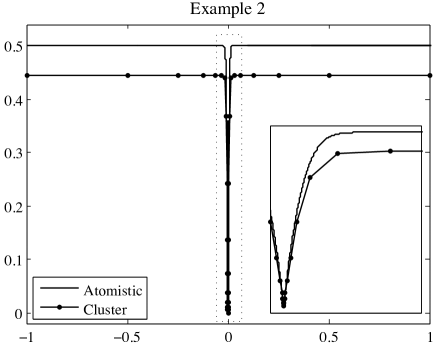
Figure 1. Computational example on a highly graded mesh with force $f(x)=10^{4}\exp(-10^{4}x^{2})$, $N=2^{14},$ and $K=15$. Since $f$ is not anti-symmetric, the solution is non-smooth at the origin (cf. Remark 1.1). The relative error in the energy norm satisfies $\|u_{h}^{\prime}-\bar{u}_{h}^{\prime}\|_{{\rm L}^{2}}/\|\bar{u}_{h}^{\prime}\|_{{\rm L}^{2}}\approx 0.11$ (that is $11\%$), which is in excellent agreement with our prediction. The relative error for the energy satisfies $(\mathcal{E}(u)-\mathcal{E}_{h}(u_{h}))/|\mathcal{E}(u)|\approx-0.13$ (that is $13\%$). Precisely as we predicted, we see that the failure in the coefficients enforces a smaller QC displacement which results in a higher energy.

3.3. Example 3: a non-smooth mesh

In the final example of our analysis of the energy-based cluster summation rule, we consider a mesh which is quasi-uniform, but not smooth. We assume that $\varepsilon\ll h$, and that

$$h_{k}={\textstyle\frac{1}{2}}h\big{(}3+(-1)^{k}\big{)},\qquad k=-K+1,\dots,K,$$ (28)

that is, we have $h_{1}=h$, $h_{2}=2h$, $h_{3}=h$, and so forth. A mesh of precisely this type will rarely be found in practise, however, it is an excellent model situation that demonstrates a source of error for non-smooth meshes.

In this situation, the coeffcients $\hat{\omega}_{k}$ satisfy

$$\hat{\omega}_{k}=\left\{\begin{array}[]{rl}-1/4,&\text{if~{}}k\text{~{}is~{}even,}\\ 1/2,&\text{if~{}}k\text{~{}is~{}odd.}\end{array}\right.$$

Suppose that $\bar{u}_{h}$ is the interpolant of a smooth function $\bar{u}$, so that $\bar{U}_{k}^{\prime}$ varies little between elements. Then the oscillatory nature of the coefficients $\hat{\omega}_{k}$, weighted according to the size of the elements, indicates that $a\approx 0$. More precisely, we have

$$h_{k}\hat{\omega}_{k}\bar{U}_{k}^{\prime}=\left\{\begin{array}[]{rl}{\textstyle\frac{1}{6}}(h_{k}\bar{U}_{k}^{\prime}+h_{k+1}\bar{U}_{k+1}^{\prime})+{\textstyle\frac{1}{6}}h_{k+1}(\bar{U}_{k+1}^{\prime}-\bar{U}_{k}^{\prime}),&k\text{~{}odd},\\ -{\textstyle\frac{1}{6}}(h_{k-1}\bar{U}_{k-1}^{\prime}+h_{k}\bar{U}_{k}^{\prime})+{\textstyle\frac{1}{6}}h_{k}(\bar{U}_{k}^{\prime}-\bar{U}_{k-1}^{\prime}),&k\text{~{}even},\end{array}\right.$$

from which we can easily deduce that $|a|\leq Ch$, where $C$ depends on the second differences of $\bar{U}_{k}$ (which we assumed to be moderately small). Some similar, algebraic manipulations show that

$$\sum_{k=-K+1}^{K}h_{k}\big{|}\hat{\omega}_{k}\bar{U}_{k}^{\prime}\big{|}^{2}={\textstyle\frac{1}{8}}\|\bar{u}_{h}^{\prime}\|_{{\rm L}^{2}}^{2}+\mathcal{O}(h),$$

and thus, we obtain

$$\rho(\bar{u}_{h})^{2}=\sum_{k=-K+1}^{K}h_{k}\big{|}\hat{\omega}_{k}\bar{U}_{k}^{\prime}\big{|}^{2}-2a^{2}\geq{\textstyle\frac{1}{8}}\|\bar{u}_{h}^{\prime}\|_{{\rm L}^{2}}^{2}-\mathcal{O}(h).$$

From our general error estimate (27), we therefore expect the relative error to be roughly of the order $1/\sqrt{8}$ (that is $35\%$), which is in excellent agreement with the numerical example shown in Figure 2.

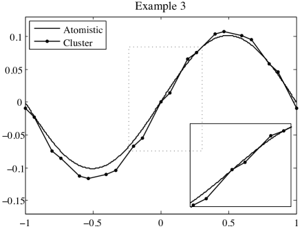
Figure 2. Computational example on an oscillatory mesh with force $f(x)=\sin(\pi x)$, $N=10^{4}$ and $K=20$. The fully atomistic solution is given by $u(x)=\pi^{-2}\sin(\pi x)$. The relative error in the energy norm satisfies $\|u_{h}^{\prime}-\bar{u}_{h}^{\prime}\|_{{\rm L}^{2}}/\|\bar{u}_{h}^{\prime}\|_{{\rm L}^{2}}\approx 0.33$ (that is $33\%$) while the relative error for the energy satisfies $(\mathcal{E}(u)-\mathcal{E}_{h}(u_{h}))/|\mathcal{E}(u)|\approx 0.097$ (that is $9.7\%$). In the zoomed box, we see that the microstructure, induced by the oscillatory coefficients, is lowering the energy and creates a ‘non-smooth’ quasicontinuum solution.

4. Conclusion

We have shown that node-based cluster summation rules, applied either to the force-based formulation of the QC method or to the energy-based formulation of the QC method lead to inconsistent and inaccurate numerical schemes when used with graded or non-smooth meshes. We stress, furthermore, that increasing the cluster size is not a remedy for the sources of error which we have discussed.

We do not rule out, however, that QC methods based on a more careful choice of summation points may yet lead to excellent computational tools. We would like to comment on three options which qualify for further investigation:

Lin’s formulation [13] and the formulation of Gunzburger & Zhang [9, 10], which are based on summation points in the interior of the elements do not suffer from any of the deficiencies which we have found in the present work. It will be necessary, however, to carefully investigate the effect of next-nearest neighbour and finite range interaction in the transition region in which the mesh is refined from large triangles to the atomistic scale where all degrees of freedom are retained.

A force-based formulation, where the summation is performed over element interfaces rather than elements may yet lead to an accurate QC method. This is clearly true in one dimension, but needs to be carefully studied in higher dimensions.

Finally, we propose to investigate the possibility of assigning variable weights to atoms within the same cluster, in an energy-based cluster summation rule. It can be readily verified, following the analogy with continuum finite element energies discussed at the end of the introduction, that if the average over atoms in a cluster is weighted according to element sizes, then the resulting method will be accurate for nearest-neighbour interaction. Once again, the crucial questions are whether this accuracy can be retained for finite range interaction and the application relevant two- three-dimensional situations.

Appendix A Proofs

A.1. Computation of summation weights

The analysis presented in this appendix applies to both the energy-based and the force-based summation rules, since the weights satisfy $\omega_{j}=\varepsilon\nu_{j}$. For no particular reason, we chose to work with the weights $(\omega_{j})_{j=-K+1}^{K}$.

We assume throughout that $r_{k}^{\pm}\equiv r$. According to the requirement (17), the governing equations for the weights $\omega=(\omega_{k})_{k=-K+1}^{K}$ are $M\omega=g$ where

$$(M\omega)_{j}:=~{} \sum_{k=-K+1}^{K}\omega_{k}\sum_{\ell\in\mathcal{C}_{k}}\zeta_{j}(\varepsilon\ell)$$

$$=~{} \omega_{j-1}\big{(}{\textstyle\frac{1}{2}}r(r+1)\varepsilon h_{j}^{-1}\big{)}+\omega_{j+1}\big{(}{\textstyle\frac{1}{2}}r(r+1)\varepsilon h_{j+1}^{-1}\big{)}$$

$$+\omega_{j}\big{(}(2r+1)-{\textstyle\frac{1}{2}}r(r+1)\varepsilon h_{j}^{-1}-{\textstyle\frac{1}{2}}r(r+1)\varepsilon h_{j+1}^{-1}\big{)}$$

and

$$g_{j}:=\sum_{\ell=-N+1}^{N}\varepsilon\zeta_{j}(\varepsilon\ell)={\textstyle\frac{1}{2}}(h_{j+1}+h_{j}).$$

To prove that $M$ is invertible, we show that it is row-diagonally dominant. For each $j,$ we have

$$M_{jj}-\sum_{k\neq j}|M_{j,k}|=(2r+1)-r(r+1)\varepsilon(h_{j}^{-1}+h_{j+1}^{-1}).$$

Since we assumed that the clusters do not overlap, it follows that $\ell_{j}-\ell_{j-1}\geq 2r+1$, in particular, $-\varepsilon r>-{\textstyle\frac{1}{2}}h_{j}$, from which we deduce that

$$M_{jj}-\sum_{k\neq j}|M_{j,k}|>(2r+1)-(r+1)=r.$$ (29)

Thus, $M$ is invertible and $\omega$ is well-defined. We note, furthermore, that (29) implies that

$$\|M^{-1}\|_{\ell^{\infty}}\leq\left\{\begin{array}[]{rl}1/r,&\text{if~{}}r\geq 1,\\ 1,&\text{if~{}}r=0.\end{array}\right.$$ (30)

Our next observation is that the lumped system for computing the approximate weights $\bar{\omega}=(\bar{\omega}_{k})_{k=-K+1}^{K}$ is

$$(2r+1)\bar{\omega}_{j}={\textstyle\frac{1}{2}}(h_{j+1}+h_{j}),\qquad j=-K+1,\dots,K,$$

that is,

$$\bar{\omega}_{j}=\frac{h_{j+1}+h_{j}}{2(2r+1)},\qquad j=-K+1,\dots,K.$$ (31)

We shall now prove that the exact weights $(\omega_{k})_{k=-K+1}^{K}$ are only $\mathcal{O}(\varepsilon)$ perturbations from the approximate weights obtained by mass-lumping. To this end, we define the residual $\rho=(\rho_{k})_{k=-K+1}^{K}$,

$$\rho_{j}:=~{} (M\bar{\omega})_{j}-g_{j}$$

$$=~{} (\bar{\omega}_{j-1}-\bar{\omega}_{j})\big{(}{\textstyle\frac{1}{2}}r(r+1)\varepsilon h_{j}^{-1}\big{)}+(\bar{\omega}_{j+1}-\bar{\omega}_{j})\big{(}{\textstyle\frac{1}{2}}r(r+1)\varepsilon h_{j+1}^{-1}\big{)}.$$

If the mesh is uniform or if $r=0$, then $\rho=0$. In general, under the mesh regularity assumption (7) we obtain the residual estimate

$$\|\rho\|_{\ell^{\infty}}\leq C(\kappa)\varepsilon r.$$ (32)

To estimate the error on the weights, we note that $M(\bar{\omega}-\omega)=\rho$, and hence

$$\|\bar{\omega}-\omega\|_{\ell^{\infty}}\leq\|M^{-1}\|_{\ell^{\infty}}\|\rho\|_{\ell^{\infty}}\leq\max(1,r)^{-1}C(\kappa)r\varepsilon,$$

that is, we obtain

$$\|\bar{\omega}-\omega\|_{\ell^{\infty}}\leq\left\{\begin{array}[]{rl}C(\kappa)\varepsilon\quad\text{if~{}}r\geq 1,\\ 0\quad\text{if~{}}r=0.\end{array}\right.$$ (33)

This may seem an impossibly strong result at first glance, however, we note that it is only true under the restriction that $r_{k}^{\pm}\equiv r$ for all $k$. We expect that, in general, the cluster size will influence the estimate to give an error of order $\mathcal{O}(\varepsilon\max r_{k}^{\pm})$.

Upon noticing that the weights for the force-based summation rule satisfy $\nu_{j}=\omega_{j}/\varepsilon$, an estimate for the weights $\nu_{j}$ follows immediately.

A.2. Proof of (15)

Let $I$ be the interpolation operator for the quasicontinuum mesh, that is, $I:\mathcal{X}\rightarrow\mathcal{X}_{h}$ with $(Iv_{h})_{\ell_{k}}=v_{h,\ell_{k}}$, $k=-K+1,\dots,K$. Let $g\in\mathcal{X}$ be given by $g_{\ell}=f_{\ell}\zeta_{j}(\varepsilon\ell)$, then

$$\sum_{\ell=-N+1}^{N}\varepsilon g_{\ell}=\sum_{-N+1}^{N}\varepsilon Ig_{\ell}+\sum_{-N+1}^{N}\varepsilon(g_{\ell}-Ig_{\ell}).$$

In view of our assumption that $f_{\ell}=\bar{f}(\varepsilon\ell),$ where $\bar{f}\in{\rm C}^{2}[-1,1]$, and the interpolation error estimate of [17, Thm A.4], it follows that

$$\sum_{\ell=-N+1}^{N}\varepsilon g_{\ell}=\sum_{-N+1}^{N}\varepsilon Ig_{\ell}+\mathcal{O}(h_{j}^{2}+h_{j+1}^{2}).$$

Since, by definition, piecewise affine functions are summed exactly by the cluster summation rule, it follows that

$$\sum_{\ell=-N+1}^{N}\varepsilon g_{\ell}=\sum_{k=-K+1}^{K}\nu_{k}\sum_{\ell\in\mathcal{C}_{k}}\varepsilon Ig_{\ell}+\mathcal{O}(h_{j}^{2}+h_{j+1}^{2}).$$

Applying the same argument as above, we can deduce that

$$\sum_{k=-K+1}^{K}\nu_{k}\sum_{\ell\in\mathcal{C}_{k}}\varepsilon Ig_{\ell}=\sum_{k=-K+1}^{K}\nu_{k}\sum_{\ell\in\mathcal{C}_{k}}\varepsilon g_{\ell}+\mathcal{O}(h_{j}^{2}+h_{j+1}^{2}),$$

from which the desired result follows.

References

• [1] P. G. Ciarlet. The finite element method for elliptic problems, volume 40 of Classics in Applied Mathematics. Society for Industrial and Applied Mathematics (SIAM), Philadelphia, PA, 2002. Reprint of the 1978 original [North-Holland, Amsterdam; MR0520174 (58 #25001)].
• [2] M. Dobson and M. Luskin. An analysis of the effect of ghost force oscillation on the quasicontinuum error. manuscript, 2008.
• [3] M. Dobson and M. Luskin. An optimal order error analysis of the one-dimensional quasicontinuum approximation. manuscript, 2008.
• [4] M. Dobson and M. Luskin. Analysis of a force-based quasicontinuum approximation. M2AN Math. Model. Numer. Anal., 42(1):113–139, 2008.
• [5] W. E, J. Lu, and J.Z. Yang. Uniform accuracy of the quasicontinuum method. Phys. Rev. B, 74(21):214115, 2004.
• [6] W. E and P. Ming. Analysis of the local quasicontinuum method. In Frontiers and prospects of contemporary applied mathematics, volume 6 of Ser. Contemp. Appl. Math. CAM, pages 18–32. Higher Ed. Press, Beijing, 2005.
• [7] W. E, P. Ming, and J. Yang. Analysis of the quasicontinuum method. manuscript, 2007.
• [8] B. Eidel and A. Stukowski. A variational formulation of the quasicontinuum method based on energy sampling in clusters. to appear in J. Mech. Phys. Solids, 2008.
• [9] M. Gunzburger and Y. Zhang. A quadrature-rule type approximation for the quasicontinuum method. manuscript, 2008.
• [10] M. Gunzburger and Y. Zhang. Quadrature-rule type approximations to the quasicontinuum method for short and long-range interatomic interactions. manuscript, 2008.
• [11] J. Knap and M. Ortiz. An Analysis of the Quasicontinuum Method. J. Mech. Phys. Solids, 49:1899–1923, 2001.
• [12] P. Lin. Theoretical and numerical analysis for the quasi-continuum approximation of a material particle model. Math. Comp., 72(242):657–675, 2003.
• [13] P. Lin. Convergence analysis of a quasi-continuum approximation for a two-dimensional material without defects. SIAM J. Numer. Anal., 45(1):313–332 (electronic), 2007.
• [14] R. Miller and E. Tadmor. Benchmarking multiscale methods. Modeling and Simulation in Materials Science and Engineering, submitted.
• [15] R.E. Miller and E.B. Tadmor. The Quasicontinuum Method: Overview, Applications and Current Directions. Journal of Computer-Aided Materials Design, 9:203–239, 2003.
• [16] M. Ortiz, R. Phillips, and E. B. Tadmor. Quasicontinuum Analysis of Defects in Solids. Philosophical Magazine A, 73(6):1529–1563, 1996.
• [17] C. Ortner and E. Süli. Analysis of a quasicontinuum method in one dimension. M2AN Math. Model. Numer. Anal., 42(1):57–91, 2008.
• [18] V. B. Shenoy, R. Miller, E. B. Tadmor, D. Rodney, R. Phillips, and M. Ortiz. An adaptive finite element approach to atomic-scale mechanics–the quasicontinuum method. J. Mech. Phys. Solids, 47(3):611–642, 1999.
• [19] T. Shimokawa, J.J. Mortensen, J. Schiotz, and K.W. Jacobsen. Matching conditions in the quasicontinuum method: Removal of the error introduced at the interface between the coarse-grained and fully atomistic region. Phys. Rev. B, 69(21):214104, 2004.