Chiral-odd generalized parton distributions,
transversity decomposition of angular momentum,
and tensor charges of the nucleon

Abstract

The forward limit of the chiral-odd generalized parton distributions (GPDs) and their lower moments are investigated within the framework of the chiral quark soliton model (CQSM), with particular emphasis upon the transversity decomposition of nucleon angular momentum proposed by Burkardt. A strong correlation between quark spin and orbital angular momentum inside the nucleon is manifest itself in the derived second moment sum rule within the CQSM, thereby providing with an additional support to the qualitative connection between chiral-odd GPDs and the Boer-Mulders effects. We further confirm isoscalar dominance of the corresponding first moment sum rule, which indicates that the Boer-Mulders functions for the $u$- and $d$-quarks have roughly equal magnitude with the same sign. Also made are some comments on the recent empirical extraction of the tensor charges of the nucleon by Anselmino et al. We demonstrate that a comparison of their result with any theoretical predictions must be done with great care, in consideration of fairly strong scale dependence of tensor charges, especially at lower renormalization scale.

I Introduction

The concept of generalized parton distributions (GPDs) has recently attracted considerable interest MRGDH94 - BR05 . Naturally, these new quantities contain richer information on the internal quark-gluon structure of the nucleon, well beyond what can be learned from the usual parton distribution functions (PDFs). A complete set of quark GPDs at the leading twist 2 contains four helicity conserving distributions, usually denoted as $H^{q},E^{q},\tilde{H}^{q},\tilde{E}^{q}$, and four helicity-flip (chiral-odd) distributions, labeled as $H_{T}^{q},E_{T}^{q},\tilde{H}_{T}^{q},\tilde{E}_{T}^{q}$ HJ98 ,Diehl01 . These GPDs are all functions of three kinematical variables, $x$, $\xi$, and $t$, where $x$ is a generalized Bjorken variable, $t$ is the four-momentum-transfer square of the nucleon, while $\xi$ is the longitudinal momentum transfer, usually called the skewdness parameter. The standard PFDs are naturally contained as a subset of these GPDs. That is, in the forward limit $\xi,\,t\rightarrow 0$ of zero momentum transfer, $H^{q}(x,\xi,t)$ and $\tilde{H}^{q}(x,\xi,t)$ reduce to the unpolarized distribution function $q(x)$, and the longitudinally polarized distribution functions $\Delta q(x)$, respectively. On the other hand, $H_{T}^{q}(x,\xi,t)$ reduces to the so-called transversity distribution function $\Delta_{T}q(x)$.

Experimental studies so far have mostly been concentrated on the helicity-conserving (chiral-even) GPDs, especially on $H^{q}(x,\xi,t)$ and $E^{q}(x,\xi,t)$ ENV06 -JLabHallA07 , because they are very interesting quantities for clarifying the role of quark orbital angular momentum in the nucleon spin problem Ji98 ,Ji97 -JTH96 and also because they are easier to access experimentally as compared with the helicity-flip (chiral-odd) GPDs. Although there exist some proposals to access to the chiral-odd GPDs in diffractive double meson production IPST02 ,IPST04 , we now have almost no empirical information on them. (An exception is the forward limit of GPD $H^{q}(x,\xi,t)$, i.e. the transversity $\Delta_{T}q(x)$. The first empirical extraction of the transversity distribution has recently been done by Anselmino et al. based on the combined global analysis of the measured azimuthal asymmetries in semi-inclusive scatterings and those in $e^{+}e^{-}\rightarrow h_{1}h_{2}X$ processes ABDKMPT07 ,ABDLMM08 .)

Although a direct experimental access to the chiral-odd GPDs is not very easy at the present moment, it was shown by Burkardt that they are not only interesting from a theoretical viewpoint but also they have important influence on some physical observables Burkardt05 ,Burkardt06 . First, the transversity decomposition of quark angular momentum in the nucleon introduced by him indicates that a strong correlation between quark spin and angular momentum is hidden in the 2nd moment of chiral-odd GPDs, more specifically in the combination $H_{T}^{q}+2\,\tilde{H}_{T}^{q}+\tilde{E}_{T}^{q}$. He also suggested that a strong correlation would exist between the 1st moment of $2\,\tilde{H}^{q}+\tilde{E}^{q}$ and the Boer-Mulders functions $h_{1}^{\perp q}$ describing the asymmetry of the transverse momentum of quarks perpendicular to the quark spin in an unpolarized target BM98 . (This is a variant of the analogous relation between the Sivers function Sivers91 and the anomalous magnetic moment of a quark with the flavor $q$ also proposed by him Burkardt04A ,Burkardt04B .)

Turning to the status of theoretical studies of chiral-odd GPDs, most works so far have been restricted to the studies of the transversity $\Delta q(x)$, which is the forward limit of the GPD $H_{T}^{q}(x,\xi,t)$. A lot of model calculations were reported on the transversity and its 1st moment, i.e. the tensor charge Olness93 -CBT08 . There also exist lattice QCD studies on the lower moments of $H_{T}^{q}(x,\xi,t)$. Its 1st moment, i.e. the tensor charge, was first investigated in ADHK97 , while the simulations were extended to include its 2nd moment as well in GHHPRSSZ05 . However, the lattice QCD studies on the moments of other GPDs, i.e. $E_{T}^{q},\tilde{H}_{T}^{q},\tilde{E}_{T}^{q}$, have not been reported yet. Concerning the full $x$, $\xi$, $t$ dependence of the chiral-odd GPDs, there have been only a few model calculations. The one is the investigation by Pasquini, Pincetti, and Boffi PPB05 -BP08 within the framework of the light-front constituent quark model (see also a similar investigation by Dahiya and Mukherjee DM08 ), and the other is the calculation by Scopetta based on a simple version of the MIT bag model. Probably, most extensive is the investigation by Pasquini et al. PPB05 . They gave predictions not only for the lower moments of GPDs but also for the full $x,\xi,t$-dependence of those GPDs. Note however that their calculations were made possible in price of one crude approximation. That is, in their model calculations, only the lowest-order Fock-space components of the light-front wave functions with three valence quarks are taken into account. The previous investigation of the chiral-even unpolarized GPD $H^{(I=0)}(x,\xi,t)$ based on the approximate treatment of the CQSM PPPBGW98 indicates that this approximation is not necessarily justified, and the inclusion of higher Fock-components may bring about richer $x$- and $\xi$-dependence in the GPDs.

In the present investigation, we try to investigate chiral-odd GPDs beyond the three valence quark approximation. Within the CQSM, which we shall use, the effects of higher Fock-space components can be included nonperturbatively as contributions of deformed Dirac-sea quarks in the hedgehog mean field DPP88 ,WY91 , not through the perturbative Fock-space expansion. Unfortunately, technical hardness of this ambitious program does not allow us complete calculation of GPDs in full dependence of the three kinematical variables, $x,\xi$ and $t$, at the present stage. In the present investigation, we therefore content ourselves in the calculation of the forward limit of a GPD, i.e. $G_{T}^{q}(x,0,0)\equiv\lim_{\xi\rightarrow 0,t\rightarrow 0}\,[\,H_{T}^{q}(x,\xi,t)+2\,\tilde{H}_{T}^{q}(x,\xi,t)+E_{T}^{q}(x,\xi,t)\,]$, since, except for the transversity distribution $H_{T}^{q}(x,0,0)$, this distribution is physically the most interesting quantity, which is thought to contain valuable information on the correlation between the quark spin and orbital angular momentum inside the nucleon as pointed out by Burkardt Burkardt05 , Burkardt06 . (There already exist several investigations within the CQSM on the forward limit of chiral-even GPD $E(x,\xi,t)$ OPSUG05 ,WT05 as well as on the generalized form factors corresponding to its lower moments WN06 -GGOPSSU07B .) Concerning the transversity $\Delta_{T}q(x)=H_{T}^{q}(x,0,0)$ contained in the combination to define $G_{T}^{q}(x,0,0)$, the first empirical information has recently obtained by Anselmino et al. through the semi-inclusive deep inelastic scatterings ABDKMPT07 ,ABDLMM08 . The extracted transversities and/or their 1st moments were compared with some model predictions. We shall discuss in the present paper, that such a comparison is potentially very dangerous if one does not pay the closest attention to the fairly strong scale dependence of the transversities.

The paper is organized as follows. First, in sect.II, we shall derive theoretical formulas, which are necessary for evaluating the relevant GPDs within the framework of the CQSM. Next, in the first part of sect.III, we show the results of numerical calculation for the isoscalar and isovector part of $G_{T}^{q}(x,0,0)$ as well as their 1st and 2nd moments. The second part of sect.III is devoted to the discussion on the delicacy, which is shown to arise in a comparison between the recent empirical determination of the tensor charges and the corresponding theoretical predictions. Some concluding remarks are then given in sect.IV.

II Chiral-odd GPDs in the CQSM

The chiral-odd GPDs are defined as nonforward matrix elements of light-cone correlation of the tensor current as

$${\cal M} = \frac{1}{2}\,\int\,\frac{dz^{-}}{2\,\pi}\,e^{i\,x\,P^{+}\,z^{-}}\,\langle p^{\prime},\lambda^{\prime}\,|\,\bar{\psi}\left(-\,\frac{z}{2}\right)\,i\,\sigma^{+j}\,\gamma_{5}\,\psi\left(-\,\frac{z}{2}\right)\,|\,p,\lambda\rangle$$ (1)

$$= \frac{1}{2\,P^{+}}\,\bar{u}(p^{\prime},\lambda^{\prime})\,\left[\,H_{T}(x,\xi,t)\,i\,\sigma^{+j}\,\gamma_{5}\ +\ \tilde{H}_{T}(x,\xi,t)\,\frac{i\,\epsilon^{+j\alpha\beta}\,\Delta_{\alpha}\,P_{\beta}}{M_{N}^{2}}\right.$$

$$\hskip 56.9055pt\left.+\ E_{T}(x,\xi,t)\,\frac{i\,\epsilon^{+j\alpha\beta}\,\Delta_{\alpha}\,\gamma_{5}}{2\,M_{N}}\ +\ \tilde{E}_{T}(x,\xi,t)\,\frac{i\,\epsilon^{+j\alpha\beta}\,P_{\alpha}\,\gamma_{\beta}}{M_{N}}\,\right]\,u(p,\lambda),$$

where $i=1,2$ is a transverse index, while $p\,(p^{\prime})$ and $\lambda\,(\lambda^{\prime})$ are the momentum and the helicity of the initial (final) nucleon, respectively. We use here the light-cone coordinates $v^{\pm}=(v^{0}\pm v^{3})\,/\,\sqrt{2}$, and $\mbox{\boldmath$v$}_{\perp}=(v^{1},v^{2})$ for any four-vector $v^{\mu}$. We also use the notation

$$P\ =\ \frac{1}{2}\,(p^{\prime}\ +\ p),\ \ \ \ \ \Delta\ =\ p^{\prime}-p.$$ (2)

As is widely known, the GPDs depends on three kinematical variables, $x$, $\xi$, and $t$, where $x$ is a generalized Bjorken variable, $t=\Delta^{2}$ is the four-momentum-transfer squared of the nucleon, and $\xi=-\,\Delta^{+}\,/\,(2\,P^{+})$ denotes the longitudinal momentum transfer, usually called the skewdness parameter.

For model calculation, it is convenient to work in the so-called Breit frame, in which

$$p^{\prime}\ =\ \left(E_{\mbox{\boldmath$\Delta$}/2},+\,\mbox{\boldmath$\Delta$}/2\right),\ \ \ \ \ p\ =\ \left(E_{\mbox{\boldmath$\Delta$}/2},-\,\mbox{\boldmath$\Delta$}/2\right),\ \ \ \ \$$ (3)

so that

$$P = \left(E_{\mbox{\boldmath$\Delta$}/2},\mbox{\boldmath$0$}\right),\ \ \ \ \ \Delta\ =\ \left(0,\mbox{\boldmath$\Delta$}\right).$$ (4)

We also assume large $N_{c}$ kinematics, in which the nucleon is heavy, $M_{N}\sim O(N_{c})$, and its center-of-mass motion is essentially nonrelativistic. Under these circumstances, $\Delta^{i}=O(N_{c}^{0})$ and $\Delta^{0}=O(N_{c}^{-1})$, so that the hierarchy holds that $M_{N}\gg|\Delta^{i}|\gg|\Delta^{0}|$. Note also that $t=-\,\mbox{\boldmath$\Delta$}=O(N_{c}^{0})$ and $\xi=-\,\Delta^{3}/(2\,M_{N})=O(N_{c}^{-1})$. Then, noting that $\mbox{\boldmath$\Delta$}=(\mbox{\boldmath$\Delta$}_{\perp},-\,2\,M_{N}\,\xi)$, we evaluate the right hand side of eq. (1), to obtain

$${\cal M} \sim \left[\,H_{T}\ +\ \frac{\mbox{\boldmath$\Delta$}_{\perp}^{2}}{8\,M_{N}^{2}}\,\left(E_{T}-\frac{1}{2}\,H_{T}\right)\ +\ \xi\,\tilde{E}_{T}\,\right]\,\sigma_{1}$$ (5)

$$+ \frac{1}{2\,M_{N}}\,\left[\,H_{T}\ +\ 2\,\tilde{H}_{T}\ +\ E_{T}\,\right]\,i\,\Delta_{2}$$

$$+ \frac{1}{2\,M_{N}}\,\tilde{E}_{T}\,\,\Delta_{1}\,\sigma_{3}$$

$$- \left[\,E_{T}\ -\ \frac{1}{2}\,H_{T}\,\right]\,\frac{1}{4\,M_{N}^{2}}\,\left\{\,\Delta_{1}\,(\mbox{\boldmath$\sigma$}\cdot\mbox{\boldmath$\Delta$}_{\perp})\ -\ \frac{1}{2}\,\mbox{\boldmath$\Delta$}_{\perp}^{2}\,\sigma_{1}\,\right\}.$$

Since we are interested in the forward limit ($\mbox{\boldmath$\Delta$}_{\perp}\rightarrow 0$, $\xi\rightarrow 0$) in the present investigation, we can project out these four independent pieces as

$$H_{T}(x,0,0) = \frac{1}{2\,\pi}\,\int_{0}^{2\,\pi}\,d\phi\,\,\,\frac{1}{2}\,\mbox{tr}\,\sigma_{1}\,{\cal M},$$ (6)

$$\frac{1}{2\,M_{N}}\,\left[\,H_{T}\ +\ 2\,\tilde{H}_{T}\ +\ E_{T}\,\right]\,(x,0,0) = \frac{1}{\pi}\,\int_{0}^{2\,\pi}\,d\phi\,\,\frac{\Delta_{2}}{i\,|\mbox{\boldmath$\Delta$}_{\perp}|^{2}}\,\,\frac{1}{2}\,\mbox{tr}\,{\cal M},$$ (7)

$$\frac{1}{2\,M_{N}}\,\tilde{E}_{T}(x,0,0) = \frac{1}{\pi}\,\int_{0}^{2\,\pi}\,\,d\phi\,\,\frac{\Delta_{1}}{|\mbox{\boldmath$\Delta$}_{\perp}|^{2}}\,\,\frac{1}{2}\,\mbox{tr}\,\sigma_{3}\,{\cal M},$$ (8)

$$-\,\frac{1}{4\,M_{N}^{2}}\,\left[\,E_{T}\ -\ \frac{1}{2}\,H_{T}\,\right]\,(x,0,0) = \frac{2}{\pi}\,\int_{0}^{2\,\pi}\,d\phi\,\,\frac{1}{|\mbox{\boldmath$\Delta$}_{\perp}|^{4}}$$ (9)

$$\times \frac{1}{2}\,\,\mbox{tr}\,\left[\,(\mbox{\boldmath$\Delta$}_{\perp}\cdot\mbox{\boldmath$\sigma$})\,\Delta_{1}\ -\ \frac{1}{2}\,\mbox{\boldmath$\Delta$}_{\perp}^{2}\,\sigma_{1}\,\right]\,{\cal M},$$

where $\phi$ is the azimuthal angle of the transverse vector $\mbox{\boldmath$\Delta$}_{\perp}$, i.e. $\mbox{\boldmath$\Delta$}_{\perp}=|\mbox{\boldmath$\Delta$}_{\perp}|\,(\cos\phi,\sin\phi)$. For convenience, let us use below the shorthand notation :

$$G_{T}(x,\xi,t) \equiv \ H_{T}(x,\xi,t)\ +\ 2\,\tilde{H}_{T}(x,\xi,t)\ +\ E_{T}(x,\xi,t),$$ (10)

$$K_{T}(x,\xi,t) \equiv \ E_{T}(x,\xi,t)\ -\ \frac{1}{2}\,H_{T}(x,\xi,t).$$ (11)

Now, we are ready to evaluate the amplitudes ${\cal M}$ explicitly in the CQSM. We first investigate the answer at the mean field level, i.e. we derive theoretical expressions for the $O(\Omega^{0})$ contribution to ${\cal M}$, with $\Omega$ being the collective angular velocity of the rotating hedgehog mean field. Using the formalism developed in the previous studies WK99 , DPPPW96 -Wakamatsu03B , the isoscalar part of ${\cal M}(x,0,t)$ at the $O(\Omega^{0})$ is given as a sum over all the occupied eigen-states of the Dirac Hamiltonian $H$ :

$${\cal M}^{(I=0)}(x,0,t) = M_{N}\,\int\,\frac{dz_{0}}{2\,\pi}\,\int\,d^{3}\mbox{\boldmath$x$}\,\,e^{\,i\,\mbox{\boldmath$\Delta$}_{\perp}\cdot\mbox{\boldmath$x$}}$$ (12)

$$\times N_{c}\,\sum_{n\in occ}\,e^{i\,z_{0}\,(x\,M_{N}-E_{n})}\,\Phi_{n}^{\dagger}(\mbox{\boldmath$x$})\,(\gamma_{1}\,\gamma_{5}-i\,\gamma_{2})\,\Phi_{n}(\mbox{\boldmath$x$}-z_{0}\,\mbox{\boldmath$e$}_{3}),$$

with $\mbox{\boldmath$e$}_{3}=(0,0,1)$ being a unit vector in the $z$ direction. Here, $\Phi_{n}(\mbox{\boldmath$X$})$ are the eigenfunctions of the Dirac hamiltonian with the hedgehog mean field, i.e.

$$H\,\Phi_{n}(\mbox{\boldmath$x$})\ =\ E_{n}\,\Phi_{n}(\mbox{\boldmath$x$}),$$ (13)

with

$$H\ =\ \frac{\mbox{\boldmath$\alpha$}\cdot\nabla}{i}\ +\ \beta\,M\,e^{i\,\gamma_{5}\,\mbox{\boldmath$\tau$}\cdot\hat{\mbox{\boldmath$r$}}\,F(r)}.$$ (14)

Noting that

$$e^{\,i\,\mbox{\boldmath$\Delta$}_{\perp}\cdot\mbox{\boldmath$x$}}\ =\ 1\ +\ i\,\mbox{\boldmath$\Delta$}_{\perp}\cdot\mbox{\boldmath$x$}\ -\ \frac{1}{2}\,(\mbox{\boldmath$\Delta$}_{\perp}\cdot\mbox{\boldmath$x$})^{2}\ +\ \cdots,$$ (15)

we easily find that

$$H_{T}^{(I=0)}(x,0,0) = 0$$ (16)

$$\frac{1}{2\,M_{N}}\,G_{T}^{(I=0)}(x,0,0) = M_{N}\,N_{c}\,\sum_{n\in occ}\,\langle n\,|\,x_{2}\,(\gamma_{1}\,\gamma_{5}-i\,\gamma_{2})\,\delta(x\,M_{N}-E_{n}-p_{3})\,|n\rangle,\hskip 28.45274pt$$ (17)

$$\frac{1}{2\,M_{N}}\,\tilde{E}_{T}^{(I=0)}(x,0,0) = 0,$$ (18)

$$\frac{1}{4\,M_{N}^{2}}\,K_{T}^{(I=0)}(x,0,0) = 0,$$ (19)

which shows that only $G_{T}^{(I=0)}(x,0,0)$ survives among the four GPDs, at the lowest order in $\Omega$, or in $1/N_{c}$ expansion.

Next, we turn to the isovector part. The isovector part of ${\cal M}(x,0,t)$ is given as

$${\cal M}^{(I=1)}(x,0,t) = M_{N}\,\int\,\frac{dz_{0}}{2\,\pi}\,\int\,d^{3}\mbox{\boldmath$x$}\,\,e^{\,i\,\mbox{\boldmath$\Delta$}_{\perp}\cdot\mbox{\boldmath$x$}}$$ (20)

$$\times N_{c}\,\sum_{n\in occ}\,e^{i\,z_{0}\,(x\,M_{N}-E_{n})}\,\Phi_{n}^{\dagger}(\mbox{\boldmath$x$})\,A^{\dagger}\,\tau_{3}\,A\,(\gamma_{1}\,\gamma_{5}-i\,\gamma_{2})\,\Phi_{n}(\mbox{\boldmath$x$}-z_{0}\,\mbox{\boldmath$e$}_{3}),\ \ \ \ \$$

where $A$ is the rotation matrix belonging to flavor $SU(2)$. Here we use the identity

$$A^{\dagger}\,\tau_{3}\,A\ =\ D_{3k}(A)\,\tau_{k},$$ (21)

where $D_{3k}(A)$ is a Wigner’s rotation matrix, which should eventually be sandwiched between the rotational wave functions $\Psi_{T_{3},J_{3}}^{(T=S=1/2)}[A]$ representing the spin-isospin states of the nucleon. Using the expansion (15), together with the replacement

$$D_{3k}(A)\ \longrightarrow\ -\,\frac{1}{3}\,\left(\tau_{3}\right)_{T_{3}^{\prime}T_{3}}\,\left(\sigma_{k}\right)_{S_{3}^{\prime}S_{3}},$$ (22)

which should be interpreted as an abbreviation of the identity

$$\int\,\Psi_{T_{3}^{\prime},S_{3}^{\prime}}^{(T=S=1/2)*}[A]\,\,D_{3k}(A)\,\,\Psi_{T_{3},S_{3}}^{(T=S=1/2)}[A]\,\,{\cal D}A\ =\ -\,\frac{1}{3}\,\left(\tau_{3}\right)_{T_{3}^{\prime}T_{3}}\,\left(\sigma_{k}\right)_{S_{3}^{\prime}S_{3}},$$ (23)

in the projection formulas (7) - (9), we are led to the following expressions for the $O(\Omega^{0})$ contributions to the isovector parts of four GPDs as

$$H_{T}^{(I=1)}(x,0,0) = M_{N}\,\left(-\,\frac{N_{c}}{3}\right)\,\sum_{n\in occ}\,\langle n\,|\,\tau_{1}\,(\gamma_{1}\,\gamma_{5}-i\,\gamma_{2})\,\delta(xM_{N}-E_{n}-p_{3})\,|\,n\rangle,\hskip 28.45274pt$$ (24)

$$\frac{1}{2\,M_{N}}\,G_{T}^{(I=1)}(x,0,0) = 0,$$ (25)

$$\frac{1}{2\,M_{N}}\,\tilde{E}_{T}^{(I=1)}(x,0,0) = M_{N}\,\left(-\,\frac{N_{c}}{3}\right)\,\sum_{n\in occ}\,\langle n\,|\,i\,x_{1}\,\tau_{3}\,(\gamma_{1}\,\gamma_{5}-i\,\gamma_{2})\,\delta(xM_{N}-E_{n}-p_{3})\,|\,n\rangle,\hskip 28.45274pt$$ (26)

$$\frac{1}{4\,M_{N}^{2}}\,K_{T}^{(I=1)}(x,0,0) = M_{N}\,\left(-\,\frac{N_{c}}{3}\right)\,\sum_{n\in occ}$$ (27)

$$\times \langle n\,|\,\frac{1}{2}\,[\,2\,(\mbox{\boldmath$x$}_{\perp}\cdot\mbox{\boldmath$\tau$})\,x_{1}-\mbox{\boldmath$x$}_{\perp}^{2}\,\tau_{1}\,]\,(\gamma_{1}\,\gamma_{5}-i\,\gamma_{2})\,\delta(xM_{N}-E_{n}-p_{3})\,|\,n\rangle.$$

Note that, just opposite to the isoscalar case, only $G_{T}^{(I=1)}(x,0,0)$ vanishes, while other three GPDs are generally nonzero.

The $O(\Omega^{1})$ contributions, or equivalently, the next-to-leading contributions in $1/N_{c}$ expansion, can similarly be evaluated, although the manipulation is much more complicated. Skipping the detailed derivation, we first write down the answers for the isoscalar parts :

$$H_{T}^{(I=0)}(x,0,0)\ =\ -\,M_{N}\,\frac{N_{c}}{2\,I}\,\sum_{m\in all,n\in occ}\,\langle m\,|\,\tau_{1}\,|\,n\rangle$$ (28)

$$\hskip 56.9055pt\times\ \langle n\,|\,(\gamma_{1}\,\gamma_{5}-i\,\gamma_{2})\,\left(\frac{1}{E_{m}-E_{n}}-\frac{1}{2\,M_{N}}\,\frac{d}{dx}\right)\,\delta(x\,M_{N}-E_{n}-p_{3})\,|\,m\rangle,$$

$$\frac{1}{2\,M_{N}}\,G_{T}^{(I=0)}(x,0,0)\ =\ 0,$$

$$\frac{1}{2\,M_{N}}\,\tilde{E}_{T}^{(I=0)}(x,0,0)\ =\ -\,M_{N}\,\frac{N_{c}}{2\,I}\,\sum_{m\in all,n\in occ}\,\langle m\,|\,\tau_{3}\,|\,n\rangle$$

$$\hskip 42.67912pt\times\ \langle n\,|\,i\,x_{1}\,(\gamma_{1}\,\gamma_{5}-i\,\gamma_{2})\,\left(\frac{1}{E_{m}-E_{n}}-\frac{1}{2\,M_{N}}\,\frac{d}{dx}\right)\,\delta(x\,M_{N}-E_{n}-p_{3})\,|\,m\rangle,\hskip 42.67912pt$$

$$\frac{1}{4\,M_{N}^{2}}\,K_{T}^{(I=0)}(x,0,0)\ =\ -\,M_{N}\,\frac{N_{c}}{2\,I}\,\sum_{m\in all,n\in occ}\,\langle m\,|\,\tau_{c}\,|\,n\rangle$$

$$\hskip 142.26378pt\times\ \,\langle n\,|\,\frac{1}{2}\,[\,(x_{1}^{2}-x_{2}^{2})\,\delta_{c,1}\ +\ 2\,x_{1}\,x_{2}\,\delta_{c,2}\,]\,(\gamma_{1}\,\gamma_{5}-i\,\gamma_{2})$$

$$\hskip 142.26378pt\times\ \left(\frac{1}{E_{m}-E_{n}}-\frac{1}{2\,M_{N}}\,\frac{d}{dx}\right)\,\delta(x\,M_{N}-E_{n}-p_{3})\,|\,m\rangle.$$ (31)

On the other hand, the $O(\Omega^{1})$ contributions to the isovector part are given as

$$H_{T}^{(I=1)}(x,0,0)\ =\ i\,\varepsilon_{1ac}\,M_{N}\,\frac{N_{c}}{6\,I}\,\sum_{m\in nocc,n\in occ}\,\frac{1}{E_{m}-E_{n}}$$

$$\hskip 142.26378pt\times\ \langle m\,|\,\tau_{c}\,|\,n\rangle\,\langle n\,|\,\tau_{a}\,(\gamma_{1}\,\gamma_{5}-i\,\gamma_{2})\,\delta(x\,M_{N}-E_{n}-p_{3})\,|\,m\rangle,$$

$$\frac{1}{2\,M_{N}}\,G_{T}^{(I=1)}(x,0,0)\ =\ -\,M_{N}\,\frac{N_{c}}{6\,I}\,\sum_{m\in all,n\in occ}\,\,\langle m\,|\,\tau_{c}\,|\,n\rangle$$

$$\hskip 42.67912pt\times\ \langle n\,|\,\tau_{c}\,x_{2}\,(\gamma_{1}\,\gamma_{5}-i\,\gamma_{2})\,\left(\frac{1}{E_{m}-E_{n}}-\frac{1}{2\,M_{N}}\,\frac{d}{dx}\right)\,\delta(x\,M_{N}-E_{n}-p_{3})\,|\,m\rangle,\hskip 28.45274pt$$

$$\frac{1}{2\,M_{N}}\,\tilde{E}_{T}^{(I=1)}(x,0,0)\ =\ i\,\varepsilon_{3ac}\,M_{N}\,\frac{N_{c}}{6\,I}\,\sum_{m\in nocc,n\in occ}\,\frac{1}{E_{m}-E_{n}}$$

$$\hskip 113.81102pt\times\ \,\langle m\,|\,\tau_{c}\,|\,n\rangle\,\langle n\,|\,\tau_{a}\,i\,x_{1}\,(\gamma_{1}\,\gamma_{5}-i\,\gamma_{2})\,\delta(x\,M_{N}-E_{n}-p_{3})\,|\,m\rangle,\hskip 28.45274pt$$

$$\frac{1}{4\,M_{N}^{2}}\,K_{T}^{(I=1)}(x,0,0)\ =\ i\,\varepsilon_{bac}\,M_{N}\,\frac{N_{c}}{6\,I}\,\sum_{m\in nocc,n\in occ}\,\frac{1}{E_{m}-E_{n}}\,\langle m\,|\,\tau_{c}\,|\,n\rangle$$

$$\hskip 28.45274pt\times\ \langle n\,|\,\tau_{a}\,\frac{1}{2}\,[\,(x_{1}^{2}-x_{2}^{2})\,\delta_{b,1}\ +\ 2\,x_{2}\,x_{2}\,\delta_{b,2}\,]\,(\gamma_{1}\,\gamma_{5}-i\,\gamma_{2})\,\delta(x\,M_{N}-E_{n}-p_{3})\,|\,m\rangle\,.$$ (35)

To sum up, we can summarize the novel $\Omega$ dependence of the eight GPDs as

$$H_{T}^{(I=0)}(x,0,0) = \ \ 0\ \ \ +\ O(\Omega^{1}),$$ (36)

$$G_{T}^{(I=0)}(x,0,0) = \ O(\Omega^{0})\ +\ 0,$$ (37)

$$\tilde{E}_{T}^{(I=0)}(x,0,0) = \ \ 0\ \ \ +\ O(\Omega^{1}),$$ (38)

$$K_{T}^{(I=0)}(x,0,0) = \ \ 0\ \ \ +\ O(\Omega^{1}),$$ (39)

and

$$H_{T}^{(I=1)}(x,0,0) = \ O(\Omega^{0})\ +\ O(\Omega^{1}),$$ (40)

$$G_{T}^{(I=1)}(x,0,0) = \ \ \ 0\ \ \ \ +\ O(\Omega^{1}),$$ (41)

$$\tilde{E}_{T}^{(I=1)}(x,0,0) = \ O(\Omega^{0})\ +\ O(\Omega^{1}),$$ (42)

$$K_{T}^{(I=1)}(x,0,0) = \ O(\Omega^{0})\ +\ O(\Omega^{1}),$$ (43)

where terms which do not contribute are denoted as $0$. Since $\Omega$ is an $O(1/N_{c})$ quantity, this especially means that $G_{T}(x,0,0)$ is a quantity with isoscalar dominance, although the isovector component also exists as an $1/N_{c}$ correction. (See the discussion in sect.III.) One may also notice that the contributions to the isovector GPDs, $H_{T}^{(I=1)}$, $\tilde{E}_{T}^{(I=1)}$, and $K_{T}^{(I=1)}$, survive at the mean-field level, or at the $O(\Omega^{0})$ level, while these GPDs receive $O(\Omega^{1})$ contributions as well. The appearance of the antisymmetric $\varepsilon$-tensor, as observed in Eqs.(40), (42) and (43), is a characteristic feature of this novel $1/N_{c}$ correction. This unique $1/N_{c}$ correction is known to play an important role for resolving the notorious underestimation problem of some isovector observables of the nucleon like the isovector axial charge and the isovector magnetic moment, inherent in the hedgehog-type soliton model WW93 , CBGPPWW94 ,Wakamatsu96 .

So far, we have derived the theoretical expressions for the forward limits of four chiral-odd GPDs, $H_{T}(x,\xi,t)$, $E_{T}(x,\xi,t)$, $\tilde{H}_{T}(x,\xi,t)$, and $\tilde{E}_{T}(x,\xi,t)$ in the CQSM. Since the forward limit of $H_{T}(x,\xi,t)$, which is known to reduce to the familiar transversity distribution $\Delta_{T}q(x)$, has already been investigated within the CQSM WK99 -Wakamatsu07 , we need to evaluate the remaining three independent GPDs, $E_{T}(x,0,0)$, $\tilde{H}_{T}(x,0,0)$, and $\tilde{E}_{T}(x,0,0)$, or equivalently, $G_{T}(x,0,0)$, $K_{T}(x,0,0)$, and $\tilde{E}_{T}(x,0,0)$. Unfortunately, we find that the numerical calculation of $K_{T}(x,0,0)$ is quite involved. In the present study, we therefore concentrate on $G_{T}(x,0,0)$, which is a special combination of three GPDs, $H_{T}(x,0,0)$, $\tilde{H}_{T}(x,0,0)$, and $E_{T}(x,0,0)$, as given by (10). From a physical viewpoint, this is the most interesting quantity, which appears in Burkardt’s transversity decomposition of quark angular momentum Burkardt05 ,Burkardt06 .

According to Burkardt, the transverse decomposition of angular momentum in the nucleon is given in the form

$$\langle J_{q}^{x}\rangle\ =\ \langle J_{q,+\hat{x}}^{x}\rangle\ +\ \langle J_{q,-\hat{x}}^{x}\rangle,$$ (44)

where the 1st and the 2nd terms in the right hand side respectively stand for the angular momentum carried by quarks with transverse polarization in the $+\,\hat{x}$ and $-\,\hat{x}$ directions in an unpolarized nucleon at rest. On the other hand, the difference of the above two quantities gives the transverse asymmetry

$$\langle\delta^{x}\,J_{q}^{x}\rangle\ =\ \langle J_{q,+\hat{x}}^{x}\rangle\ -\ \langle J_{q,-\hat{x}}^{x}\rangle,$$ (45)

which can be interpreted as representing a correlation between quark spin and orbital angular momentum in an unpolarized nucleon. Burkardt has derived the identities, which relate the above two quantities to the 1st and the 2nd moment of GPDs as

$$\langle J_{q}^{x}\rangle = \frac{S^{x}}{2}\,\int_{-1}^{1}\,\left[\,H(x,0,0)\ +\ E(x,0,0)\,\right]\,dx$$ (46)

$$\langle\delta J_{q}^{x}\rangle = \frac{1}{2}\,\int_{-1}^{1}\,x\,\left[\,H_{T}(x,0,0)\ +\ 2\,\tilde{H}_{T}(x,0,0)\ +\ E_{T}(x,0,0)\,\right]\,dx$$ (47)

$$= \frac{1}{2}\,\int_{=1}^{1}\,x\,G_{T}(x,0,0)\,dx.$$

The quantities appearing in the 1st sum rule are the forward limit of the familiar (chiral-even) unpolarized GPDs, $H(x,\xi,t)$ and $E(x,\xi,t)$. This identity is essentially Ji’s nucleon spin sum rule and nothing new Ji98 . What is new is the second sum rule. It relates the above-mentioned transverse asymmetry to the 2nd moment of the chiral-odd GPD $G_{T}$, which we recall is a particular combination of $H_{T}$, $\tilde{H}_{T}$, and $E_{T}$. It is interesting to see the explicit form for the 2nd moment of $G_{T}^{(I=0)}(x,0,0)$ in the CQSM. From (17), we readily find that

$$\int_{-1}^{1}\,x\,G_{T}^{(I=0)}(x,0,0)\,dx$$ (52)

$$=\,\frac{2}{3}\,N_{c}\,\sum_{n\in occ}\,\left\{\,E_{n}\,\langle n\,|\,(-\,i)\,\mbox{\boldmath$\gamma$}\cdot\mbox{\boldmath$x$}\,|\,n\rangle\ +\ \frac{1}{2}\,\langle n\,|\,\gamma^{0}\,\mbox{\boldmath$\Sigma$}\cdot\mbox{\boldmath$L$}\,|\,n\rangle\,\right\}$$

$$=\,\frac{2}{3}\,N_{c}\,\sum_{n\in occ}\,\left\{\,E_{n}\,\langle n\,|\,\left(\begin{array}[]{cc}0&\,-\,i\,\mbox{\boldmath$\sigma$}\cdot\mbox{\boldmath$x$}\\ i\,\mbox{\boldmath$\sigma$}\cdot\mbox{\boldmath$x$}&0\\ \end{array}\right)\,|\,n\rangle\ +\ \frac{1}{2}\,\langle n\,|\,\left(\begin{array}[]{cc}\mbox{\boldmath$\sigma$}\cdot\mbox{\boldmath$L$}&0\\ 0&-\,\mbox{\boldmath$\sigma$}\cdot\mbox{\boldmath$L$}\\ \end{array}\right)\,|\,n\rangle\,\right\},\ \ \ \ \$$

with $\mbox{\boldmath$\Sigma$}\equiv\gamma^{0}\,\mbox{\boldmath$\gamma$}\,\gamma_{5}$ being the relativistic spin operator of quark field. As argued by Burkardt, the transverse asymmetry signals the correlation between quark spin and orbital angular momentum in an unpolarized target. One can clearly see that such correlation manifests itself in the 2nd term of the above sum rule (52), since it reduces to the nucleon matrix element (at the mean-field level) of the operator $\gamma^{0}\,\mbox{\boldmath$\Sigma$}\cdot\mbox{\boldmath$L$}$, which is certainly the scalar product of the relativistic spin and orbital angular momentum of quarks aside from an extra factor $\gamma^{0}$. Unfortunately, the 1st term of eq.(52) is a highly model dependent expression, as convinced from the appearance of the single-particle energy $E_{n}$ of the Dirac Hamiltonian $H$ with the hedgehog mean field. This makes a simple physical interpretation of the 1st term not so easy.

Before ending this section, we want to make a brief comment on the GPD $\tilde{E}_{T}(x,\xi,t)$. Although this GPD is generally nonzero (see Eqs. (26), (II), and (II)), its 1st moment is known to vanish by time reversal invariance Diehl01 . As a consistency check of our theoretical framework, we shall explicitly prove in Appendix that the 1st moment of $\tilde{E}_{T}(x,0,0)$ in fact vanishes identically.

III Numerical results and discussions

III.1 chiral-odd GPDs and transversity decomposition of angular momentum

Within the framework of the CQSM, the expression of any nucleon observable is divided into two parts, i.e. the contribution of what-we-call the valence quark level (it is the lowest energy eigenstate of a Dirac equation with the hedgehog mean field, which emerges from the positive energy continuum) and that of the deformed Dirac sea quarks. Since the latter contains ultraviolet divergences, it must be regularized. Here, we use the Pauli-Villars regularization scheme with single subtraction, for simplicity DPPPW96 -WK99 . The Pauli-Villars regulator mass $M_{PV}$ is not an adjustable parameter of the model. It is uniquely determined from a model consistency, once the dynamical quark mass $M$, the only one parameter of the CQSM, is fixed to be $M=375\,\mbox{MeV}$ from the phenomenology of the nucleon low energy observables.

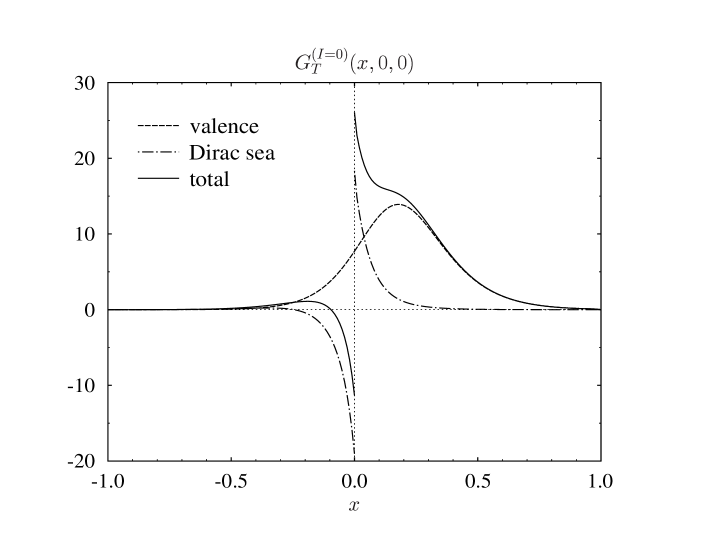
Figure 1: The prediction of the CQSM for the forward limit of the isoscalar GPD $G_{T}^{(I=0)}(x,0,0)\equiv\lim_{\xi\rightarrow 0,t\rightarrow 0}\,[\,H_{T}^{(I=0)}(x,\xi,t)+2\,\tilde{H}_{T}^{(I=0)}(x,\xi,t)+E_{T}^{(I=0)}(x,\xi,t)\,]$. The dashed and dotted curves respectively stand for the contributions of $N_{c}\,(\,=3)$ valence quarks and of deformed Dirac-sea quarks, while their sum is shown by the solid curve.

We first show in Fig.1 the CQSM predictions for the forward limit of the isoscalar GPD $G_{T}^{(I=0)}(x,\xi,t)$, i.e. $G_{T}^{(I=0)}(x,0,0)\ \equiv\ \lim_{\xi\rightarrow 0,t\rightarrow 0}\,[\,H_{T}^{(I=0)}(x,\xi,t)\ +\ 2\,\tilde{H}_{T}^{(I=0)}(x,\xi,t)\ +\ E_{T}^{(I=0)}(x,\xi,t)\,]$. Here, the dashed and dash-dotted curves respectively stand for the contribution of $N_{c}\,(\,=3\,)$ valence quarks and that of deformed Dirac-sea quarks, while their sum is shown by the solid curve. The distribution function in the negative $x$ region should be interpreted as antiquark distribution except for an extra minus sign related to the charge-conjugation property of this distribution. One clearly sees a strong chiral enhancement of the deformed Dirac-sea contribution in the small $x$ region. We recall the fact that a similar chiral enhancement of the Dirac-sea contribution is also observed in the CQSM prediction for more familiar unpolarized parton distribution function of isoscalar type, and that it plays a crucial role for ensuring the positivity condition of the antiquark distribution $\bar{u}(x)+\bar{d}(x)$ DPPPW96 ,DPPPW97 . Naturally, such chiral enhancement of the antiquark distribution cannot be reproduced by such a model as light-cone constituent quark model with $N_{c}\,(\,=3)$ quark approximation.

Next, shown in Fig.2 is the CQSM prediction for the forward limit of the isovector GPD $G_{T}^{(I=1)}(x,\xi,t)$, i.e. $G_{T}^{(I=1)}(x,0,0)\ \equiv\ \lim_{\xi\rightarrow 0,t\rightarrow 0}\,[\,H_{T}^{(I=1)}(x,\xi,t)\ +\ 2\,\tilde{H}_{T}^{(I=1)}(x,\xi,t)\ +\ E_{T}^{(I=1)}(x,\xi,t)\,]$. Here, the meaning of the curves is the same as in the previous figure. Also for the isovector distribution, one observes a strong chiral enhancement of the deformed Dirac-sea contribution in the small $x$ region. The $x$ dependence of the Dirac-sea contribution for this isovector distribution turns out to be totally different from the isoscalar distribution, however. The deformed Dirac-sea contribution for the isovector distribution is nearly symmetric with respect to the variable change $x\rightarrow-\,x$, in sharp contrast to the isoscalar distribution, which is approximately antisymmetric. This behavior is again resembling more familiar unpolarized parton distribution function of isovector type WK98 ,PPGWW99 , Wakamatsu03A . We recall the fact that this chiral enhancement of the isovector unpolarized distribution is just what is required by the celebrated NMC measurement, which established the dominance of $\bar{d}$ sea over the $\bar{u}$ sea inside the proton NMC91 . Unfortunately, we do not have any simple explanation about why such a similarity exists between the small $x$ behaviors of the unpolarized parton distribution functions $q(x)$ and the forward limit of the GPD $G_{T}(x,\xi,t)$.

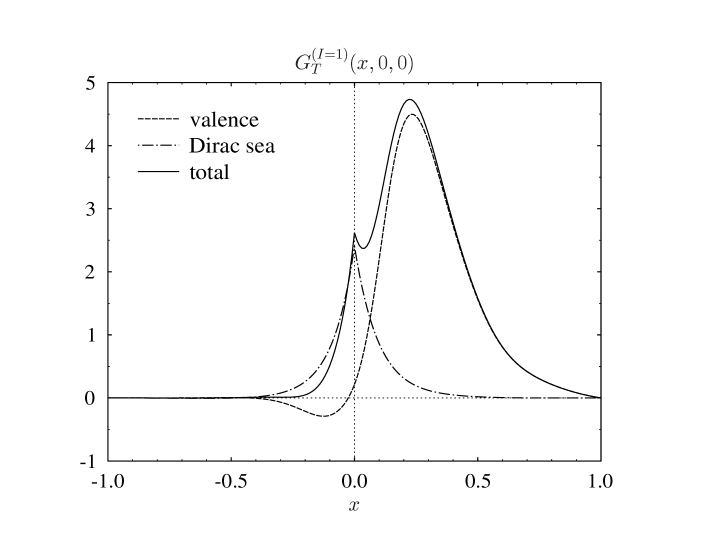
Figure 2: The prediction of the CQSM for the forward limit of the isovector GPD $G_{T}^{(I=1)}(x,0,0)\equiv\lim_{\xi\rightarrow 0,t\rightarrow 0}\,[\,H_{T}^{(I=1)}(x,\xi,t)+2\,\tilde{H}_{T}^{(I=1)}(x,\xi,t)+E_{T}^{(I=1)}(x,\xi,t)\,]$. The meaning of the curves is the same as in Fig.1.

As discussed before, the above two distribution, i.e, $G_{T}^{(I=0)}(x,0,0)$ and $G_{T}^{(I=1)}(x,0,0)$, are very interesting quantities from a physical viewpoint, since they give the transversity decomposition of the angular momentum inside the nucleon. So far, there exist only a few theoretical investigations on the chiral-odd GPDs and their moments. In table 1, we compare the CQSM predictions for the transverse asymmetries with those of the two versions of the light-front constituent quark model by Pasquini et al., that is the harmonic oscillator (HO) model and the hyper central model PPB05 . Note that their models are essentially the three quark model with relativistic kinematics. One finds that the predictions of the CQSM just lie between the HO model and the hyper central model. In all the three models, the isoscalar transverse asymmetry is seen to be larger than the isovector one, but the isoscalar-to-isovector ratio is largest in the CQSM. This observation is qualitatively consistent with the large $N_{c}$ prediction given in Pobylitsa05 . However, literally taking the $N_{c}\rightarrow\infty$ limit, the ratio $\langle\delta^{x}J_{x}^{u+d}\rangle\,/\,\langle\delta^{x}J_{x}^{u-d}\rangle$ would become infinite. Our present analysis here shows that $G_{T}(x,\xi,t)$ is an isoscalar-dominant quantity but the isovector component, which arises as a $1/N_{c}$ correction, is also important.

transverse asymmetry	HO	Hypercentral	CQSM
$\langle\delta^{x}J_{x}^{u}\rangle$	0.68	0.39	0.49
$\langle\delta^{x}J_{x}^{d}\rangle$	0.28	0.10	0.22
$2\,\langle\delta^{x}J_{x}^{u+d}\rangle$	1.92	0.98	1.41
$2\,\langle\delta^{x}J_{x}^{u-d}\rangle$	0.80	0.58	0.54
$\langle\delta^{x}J_{x}^{u+d}\rangle\,/\,\langle\delta^{x}J_{x}^{u-d}\rangle$	2.40	1.69	2.61

Table 1: Some theoretical predictions for the transverse asymmetry. Here, the second and the third columns stand for the two versions of the light-front constituent quark model of Pasquini et al. PPB05 , i.e. the harmonic oscillator model (HO) and the hyper central model (HYP), while the predictions of the CQSM are shown in the fourth column.

Also interesting is the 1st moment sum rule for $G_{T}$, which can be divided into two pieces, i.e. the 1st moment of the transversity $H_{T}^{q}(x,0,0)$ and that of the distribution $2\,\tilde{H}_{T}^{q}(x,0,0)+E_{T}^{q}(x,0,0)$ as

$$\int_{-1}^{1}\,G_{T}^{q}(x,0,0)\,dx = \int_{-1}^{1}\,H_{T}^{q}(x,0,0)\,dx\ +\ \int_{-1}^{1}\,[\,2\,\tilde{H}_{T}^{q}(x,0,0)\ +\ E_{T}^{q}(x,0,0)\,]\,dx.$$ (53)

Here, the 1st term of the r.h.s. of the above equation, i.e. the 1st moment of the transversity, gives the tensor charge

$$\Delta_{T}q\ =\ \int_{-1}^{1}\,H_{T}^{q}(x,0,0)\,dx.$$ (54)

On the other hand, the 2nd term, i.e. the 1st moment of $2\,\tilde{H}_{T}^{q}(x,0,0)+E_{T}^{q}(x,0,0)$ defined by

$$\kappa_{T}^{q}\ =\ \int_{-1}^{1}\,[\,2\,\tilde{H}_{T}^{q}(x,0,0)\ +\ E_{T}^{q}(x,0,0)\,]\,dx,$$ (55)

was given an interpretation as a quantity governing the transverse spin-flavor dipole moment in an unpolarized target by Burkardt. In fact, he showed that $\kappa_{T}^{q}$ gives us an information on how far and in which direction the average position of quarks with spin in the $\hat{x}$ direction for an unpolarized target relative to the center of momentum. The decomposition (53) corresponds to a similar decomposition of the 1st moment sum rule for the unpolarized GPD, $E_{M}^{q}(x,\xi,t)\equiv H^{q}(x,\xi,t)+E^{q}(x,\xi,t)$, which gives the total magnetic moment consisting of the quark number $N^{q}$ and the anomalous magnetic moment $\kappa^{q}$ as

$$\int_{-1}^{1}\,E_{M}^{q}(x,0,0)\,dx = \int_{-1}^{1}\,H^{q}(x,0,0)\,dx\ +\ \int_{-1}^{1}\,E^{q}(x,0,0)\,dx\ =\ \ \ N^{q}\ +\ \kappa^{q}.$$ (56)

In table 2, we again compare the CQSM predictions for the quantities $\kappa_{T}^{q}$ (here we tentatively call it the “anomalous tensor moment”) with the corresponding predictions of Pasquini et al. Here, the prediction for the isoscalar part is closer to that of the HO model, while the prediction for the isovector part is closer to that of the hyper central model.

1st moment of $2\,\tilde{H}_{T}+E_{T}$	HO	Hypercentral	CQSM
$\kappa_{T}^{u}$	3.60	1.98	3.47
$\kappa_{T}^{d}$	2.36	1.17	2.60
$\kappa_{T}^{u+d}$	5.96	3.15	6.07
$\kappa_{T}^{u-d}$	1.24	0.81	0.88
$\kappa_{T}^{u+d}\,/\,\kappa_{T}^{u-d}$	4.81	3.89	6.90

Table 2: The theoretical predictions for the 1st moment of $2\,\tilde{H}_{T}+E_{T}$.

According to Burkardt’s conjecture, one would expect an intimate connection between the time-reversal-odd (T-odd) transverse momentum-dependent distributions and the GPDs. They are the approximate proportionality relation between Siver’s function and the anomalous magnetic moment with opposite sign Burkardt04A ,Burkardt04B ,

$$f_{1}^{\perp q}(x,\mbox{\boldmath k}_{\perp}^{2})\ \sim\ -\,\kappa^{q},$$ (57)

and also the proportionality relation between Boer-Mulders’ function and the anomalous tensor moment Burkardt05 ,Burkardt06 ,

$$h_{1}^{\perp q}(x,\mbox{\boldmath k}_{\perp}^{2})\ \sim\ -\,\kappa_{T}^{q}.$$ (58)

If his conjecture is combined with with some typical model predictions for the anomalous tensor moments, one would get the following approximate relations :

$$h_{1}^{\perp d}\ \sim\ \frac{1}{2}\,h_{1}^{\perp u}\ \ : \ \ \mbox{MIT bag model},$$

$$h_{1}^{\perp d}\ \sim\ h_{1}^{\perp u}\ \ \ \ : \ \ \mbox{Large $N_{c}$ prediction},$$

$$h_{1}^{\perp d}\ \sim\ \frac{3}{4}\,h_{1}^{\perp u}\ \ : \ \ \mbox{CQSM},$$

thereby dictating that the Boer-Mulders functions for the $u$- and $d$-quarks would have the same sign, although the predictions on the relative magnitudes are a little variant. This should be contrasted with the fact that Sivers functions for the $u$- and $d$-quarks appears to have opposite sign as

$$f_{1}^{\perp d}\ \sim\ -\,f_{1}^{\perp u},$$ (59)

in conformity with empirically known relation

$$\kappa^{d}\ \sim\ -\,\kappa^{u}.$$ (60)

From our viewpoint, the origin of this qualitative difference is very simple. It comes from the fact that the anomalous magnetic moment is a quantity with isovector dominance, whereas the quantities $\kappa_{T}^{q}$ is of isoscalar dominance, as expected from the $N_{c}$ counting rule indicated in Eqs.(36)-(39).

III.2 tensor charges : current empirical information versus theoretical predictions

Some years ago, the first empirical extraction of the transversity distributions has been made by Anselmino et al. based on the combined global analysis of the measured azimuthal asymmetries in semi-inclusive deep inelastic scatterings (SIDIS) and those in $e^{+}e^{-}\rightarrow h_{1}h_{2}X$ processes. More recently, they have further refined their global analysis by using new data from HERMES, COMPASS, and BELLE Collaborations ABDLMM08 . The 1st $x$-moments of the transversity distributions - related to the tensor charge - have been extracted to be

$$\Delta_{T}u\ =\ 0.59\ \begin{array}[]{l}\raisebox{-1.72218pt}[0.0pt]{+ \,0.14}\\ \raisebox{1.72218pt}[0.0pt]{\,-- \,\,0.13}\\ \end{array},\ \ \ \ \ \Delta_{T}d\ =\ -\,0.20\ \begin{array}[]{l}\raisebox{-1.72218pt}[0.0pt]{+ \,0.05}\\ \raisebox{1.72218pt}[0.0pt]{\,-- \,\,0.07}\\ \end{array},$$ (61)

at the renormalization scale $Q^{2}=0.8\,\mbox{GeV}^{2}$. They concluded that their new transversity distributions are close to some model predictions, especially the predictions by a covariant quark-diquark model by Cloët at al. CBT08 . This agreement is related to the fact that the predictions by Cloët et al. give the smallest magnitudes of tensor charges among many theoretical predictions including those of the lattice QCD. As we shall discuss below, this statement appears very misleading, however. A delicate point is that the tensor charges are strongly scale-dependent quantities especially at low renormalization scale. In fact, the bare predictions of the covariant quark-diquark model given in CBT08 for the tensor charges are nothing small. They are

$$\Delta_{T}u\ =\ 1.04,\ \ \ \ \ \Delta_{T}d\ =\ -\,0.24,$$ (62)

or in the isospin language,

$$\Delta_{T}\,q^{(I=1)}\ =\ 1.28,\ \ \ \ \ \Delta_{T}\,q^{(I=0)}\ =\ 0.80.$$ (63)

Cloët et al. regard the transversity distributions, which give the above 1st moments, as initial distributions given at the scale $Q^{2}=0.16\,\mbox{GeV}^{2}$, and take account of their scale dependencies by using the next-to-leading (NLO) evolution equation. This procedure gives the tensor charges at the scale $Q^{2}=0.4\,\mbox{GeV}^{2}$ :

$$\Delta_{T}u\ =\ 0.69,\ \ \ \ \ \Delta_{T}d\ =\ -\,0.16,$$ (64)

or equivalently

$$\Delta_{T}q^{(I=1)}\ =\ 0.85,\ \ \ \ \ \Delta_{T}q^{(I=0)}\ =\ 0.53,$$ (65)

which are much smaller than the bare predictions of the model despite pretty small scale difference.

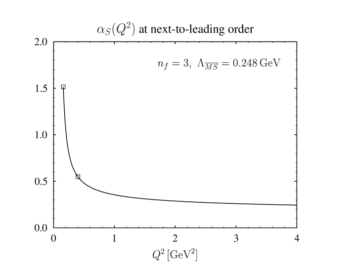
Figure 3: The QCD running coupling constant $\alpha_{S}(Q^{2})$ at the NLO in dependence of $Q^{2}$, obtained with the effective flavor number $n_{f}=3$ and the QCD scale parameter $\Lambda_{\overline{MS}}=0.248\,\mbox{GeV}$. The energy scale $Q^{2}=0.16\,\mbox{GeV}^{2}$ and $Q^{2}=0.40\,\mbox{GeV}^{2}$ are marked by open squares as a guide.

As naturally anticipated, to start the NLO evolution at such low energy scale as $Q^{2}=0.16\,\mbox{GeV}^{2}$ is very dangerous. To convince it more concretely, we first show in Fig.3 the QCD running coupling constant $\alpha_{S}(Q^{2})$ at the NLO as a function of $Q^{2}$. Here, we have used the standard NLO formula

$$\alpha_{S}^{NLO}(Q^{2})\ =\ \frac{4\,\pi}{\beta_{0}\,\ln(Q^{2}/\Lambda^{2})}\,\left[\,1\ -\ \frac{\beta_{1}}{\beta_{0}^{2}}\,\frac{\ln\ln(Q^{2}/\Lambda^{2})}{\ln(Q^{2}/\Lambda^{2})}\,\right],$$ (66)

where

$$\beta_{0}\ =\ 11\ -\ \frac{2}{3}\,n_{f},\ \ \ \ \beta_{1}\ =\ 102\ -\ \frac{38}{3}\,n_{f},$$ (67)

together with the effective flavor number $n_{f}=3$ and the QCD scale parameter $\Lambda=\Lambda_{\overline{MS}}=0.248\,\mbox{GeV}$, taken from the NLO analysis by Glück, Reya, and Vogt GRV95 . One sees that, at $Q^{2}=0.16\,\mbox{GeV}^{2}$, $\alpha_{S}(Q^{2})$ is about 1.5, which immediately throw doubt on the use of the perturbative QCD evolution equation.

The statement can be made more explicit by investigating the NLO evolution of the tensor charges themselves. The anomalous dimensions at the NLO, which control the scale dependencies of the moments of the transversities are given in KM97 ,HKK97 ,Vogelsang98 . We are interested here in the NLO evolution of the 1st moment, i.e. the tensor charges. (Note that, since the transversities do not couple to the gluon distributions, the evolution of the tensor charges is flavor independent. For more detail, see the discussion later.) The solution of the NLO evolution equation for the tensor charge $\Delta_{T}q(Q^{2})$ is given as

$$\frac{\Delta_{T}\,q(Q^{2})}{\Delta_{T}\,q(\mu^{2})}\ =\ \left(\frac{\alpha_{S}(Q^{2})}{\alpha_{S}(\mu^{2})}\right)^{\gamma^{(0)}/2\beta_{0}}\,\,\left[\,\frac{\beta_{0}\ +\ \beta_{1}\,\alpha_{S}(Q^{2})/4\,\pi}{\beta_{0}\ +\ \beta_{1}\,\alpha_{S}(\mu^{2})/4\,\pi}\,\right]^{\frac{1}{2}\,\left(\,\gamma^{(1)}/\beta_{1}\ -\ \gamma^{(0)}/\beta_{0}\right)},$$ (68)

with

$$\gamma^{(1)}/2\beta_{1} = \left(\,\frac{724}{9}\ -\ \frac{104}{27}\,n_{f}\,\right)\,/\,2\,\left(\,102\ -\ \frac{38}{3}\,n_{f}\,\right),$$ (69)

$$\gamma^{(0)}/2\beta_{0} = 4\,/\,\left(\,33-2\,n_{f}\,\right).$$ (70)

To NLO accuracy, the above solution are sometimes expanded as

$$\frac{\Delta_{T}q(Q^{2})}{\Delta_{T}q(\mu^{2})} = \left(\frac{\alpha_{S}(Q^{2})}{\alpha_{S}(\mu^{2})}\right)^{\gamma^{(0)}/2\beta_{0}}\,\left\{\,1\ -\ \frac{1}{4\,\pi}\,\frac{\beta_{1}}{\beta_{0}}\,\left(\,\frac{\gamma^{(1)}}{2\,\beta_{1}}-\frac{\gamma^{(0)}}{2\,\beta_{0}}\,\right)\,[\,\alpha_{S}(\mu^{2})\,-\,\alpha_{S}(Q^{2})\,]\,\right\}\ \ \$$ (71)

$$= \left(\frac{\alpha_{S}(Q^{2})}{\alpha_{S}(\mu^{2})}\right)^{4/27}\,\,\left\{\,1\ -\ \frac{337}{486\,\pi}\,[\,\alpha_{S}(\mu^{2})\,-\,\alpha_{S}(Q^{2})\,]\,\right\}.$$

Here, we have set $n_{f}=3$, which reproduces the form used in CBT08 . For large enough $Q^{2}$, where the QCD running coupling constant is much smaller than unity, both expressions should approximately be equivalent. However, we have already pointed out that, at the scale of $Q^{2}=0.16\,\mbox{GeV}^{2}$, $\alpha_{S}$ is even larger than 1.5.

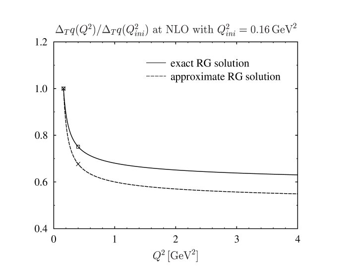
Figure 4: The scale dependence of the tensor charge, where the evolution is started at $\mu^{2}=Q_{ini}^{2}=0.16\,\mbox{GeV}^{2}$. The solid and dashed curves respectively correspond to the results obtained with the exact (Eq.(68)) and approximate (Eq.(71) solution of the NLO evolution equation.

Shown in Fig.4 are the $Q^{2}$-dependence of tensor charge, in which the evolution is started at $\mu^{2}=Q_{ini}^{2}=0.16\,\mbox{GeV}^{2}$. The solid and dashed curves respectively correspond to the answers obtained by using the exact (Eq.(68)) and approximate (Eq.(71)) solutions of the NLO evolution equation. One clearly observes a drastic difference between the two choices.

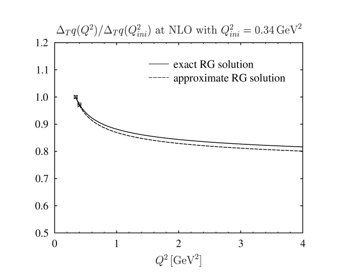
Figure 5: The scale dependence of the tensor charge, where the evolution is started at $\mu^{2}=Q_{ini}^{2}=0.34\,\mbox{GeV}^{2}$. The solid and dashed curves respectively correspond to the results obtained with the exact (Eq.(68)) and approximate (Eq.(71)) solution of the NLO evolution equation.

On the other hand, shown in Fig.5 are the $Q^{2}$ dependence of the same quantity, where the evolution is started at $\mu^{2}=Q_{ini}^{2}=0.34\,\mbox{GeV}^{2}$, which corresponds to the choice adopted in the well-known NLO analysis of the parton distribution functions by Glück, Reya and Vogt. The difference between the two forms of NLO evolution solutions is fairly small, in this case. One might suspect that not only the scale $Q_{ini}^{2}=0.16\,\mbox{GeV}^{2}$ but also the scale $Q_{ini}^{2}=0.34\,\mbox{GeV}^{2}$ is not high enough for the perturbative QCD framework to be justified perfectly. This cannot be denied completely. Still, it is clear from our simple analysis that there is a qualitative difference between the two choices of the starting energy, i.e. $Q_{ini}^{2}=0.16\,\mbox{GeV}^{2}$ and $Q_{ini}^{2}=0.34\,\mbox{GeV}^{2}$. As already pointed out, the authors of CBT08 use an approximate solution of the NLO evolution equation with the choice $Q_{ini}^{2}=0.16\,\mbox{GeV}^{2}$ to estimate the tensor charges at the scale $Q^{2}=0.40\,\mbox{GeV}^{2}$. The reduction of the magnitude of tensor charge after this scale change is significant. It is about 0.75 if one uses Eq.(68), while it is about 0.67 if one uses Eq.(71). (See the open squares and the crosses in Fig.4.) Undoubtedly, this enormous reduction has nothing to do with the nature of their effective model. It is simply a consequence of starting the NLO evolution equation at such a low energy scale.

Generally, for any effective models of baryons, it is very hard to say exactly what energy scale the predictions of those correspond to. Probably, the best we can do at the moment is to follow the spirit of PDF fit by Glück et al. GRV95 , and use the predictions of those models as initial-scale distributions given at the energy scale around $600\,\mbox{MeV}$, or $Q_{ini}^{2}\simeq(0.3-0.4)\,\mbox{GeV}^{2}$. In fact, such approach with use of the predictions of the CQSM has achieved remarkable phenomenological success for both of the unpolarized and longitudinally polarized PDFs WK99 ,Wakamatsu03A . In the following, we shall therefore use the exact solution (68) of the NLO evolution equation with the starting energy $Q_{ini}^{2}=0.34\,\mbox{GeV}^{2}$ to estimate the tensor charges at a desired scale from the predictions of low energy models.

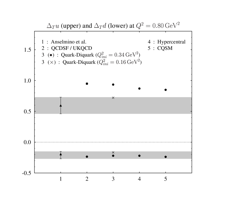
Figure 6: Comparison of empirical and theoretical tensor charges for the $u$- and $d$-quarks. The 1st column and the shaded band stand for the recent empirical determination of the $u$- and $d$-quark tensor charges by Anselmino et al., corresponding to the renormalization scale $Q^{2}=0.8\,\mbox{GeV}^{2}$. The theoretical predictions shown in other columns are all transformed to the same renormalization scale with use of the NLO evolution equation (68). See the text, for more detail.

In Fig.6, we compare the 1st empirical information on the tensor charges for the $u$- and $d$-quarks at the renormalization scale $Q^{2}=0.8\,\mbox{GeV}^{2}$ obtained by Anselmino et al. with the predictions of some low energy models as well as that of the lattice QCD. They all correspond to the scale $Q^{2}=0.8\,\mbox{GeV}^{2}$. For all the low energy models except for the covariant quark-diquark model of CBT08 , the starting energy of the evolution was taken to be $Q_{ini}^{2}=0.34\,\mbox{GeV}^{2}$ following the discussion above. In the case of the covariant quark-diquark model, we have tried two choices of the starting energy, i.e. $Q_{ini}^{2}=0.16\,\mbox{GeV}^{2}$ and $Q_{ini}^{2}=0.34\,\mbox{GeV}^{2}$. On the other hand, the predictions of the lattice QCD are given in GHHPRSSZ05 as

$$\Delta_{T}u\ =\ 0.857\pm 0.013,\ \ \ \ \Delta_{T}d\ =\ -\,0.212\pm 0.005,$$

or

$$\Delta_{T}\,q^{(I-1)}\ =\ 1.069\pm 0.018,\ \ \ \ \Delta_{T}\,q^{(I=0)}\ =\ 0.645\pm 0.018.$$

Since these predictions correspond to the renormalization scale $Q^{2}=4\,\mbox{GeV}^{2}$, we evolve those down by using eq.(68) to obtain the corresponding values at $Q^{2}=0.8\,\mbox{GeV}^{2}$. One sees that all the theoretical predictions for the $d$-quark tensor charge are not largely different and lie within the allowed range of phenomenological extraction. On the other hand, almost all the theoretical predictions for $\Delta_{T}u$ are larger in magnitude than the empirical one, thereby running off the allowed range of the empirical extraction. The prediction of the covariant quark-diquark model with use of the starting energy $Q_{ini}^{2}=0.16\,\mbox{GeV}^{2}$ is an exception. However, we have already pointed out a serious problem of using such a low starting energy.

At any rate, since the choice of the starting energy for low energy models is rather arbitrary, one must be very careful when making a comparison between model predictions for the tensor charges (or more generally transversity distribution) with phenomenologically extracted ones. (This should be contrasted with the case of axial charges. As is widely known, the isovector axial charge is known to be scale independent as a consequence of current conservation. The isoscalar or flavor-singlet axial charge is generally scale dependent, for example, in the standard $\overline{\rm MS}$ factorization scheme, because of the $U_{A}(1)$ anomaly of QCD AR88 -ET88 . However, this scale dependence is known to be fairly weak except very low energy.) Fortunately, we can avoid this troublesome problem of initial scale choice. The key point is that, since the gluon does not couple to the chiral-odd transversities, the evolutions of tensor charges are flavor independent. This in turn means that the ratio of two tensor charges as $\Delta_{T}d/\Delta_{T}u$ or $\Delta_{T}q^{(I=0)}/\Delta_{T}q^{(I=1)}$ is totally scale independent.

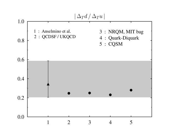
Figure 7: Comparison of empirical and theoretical tensor charge ratio $\Delta_{T}d/\Delta_{T}u$, which is scale independent.

Shown in Fig.7 is the empirically extracted tensor-charge ratio $|\Delta_{T}d/\Delta_{T}u|$ by Anselmino et al. in comparison with several theoretical predictions, i.e. those of lattice QCD GHHPRSSZ05 , non relativistic quark model (NRQM) or the MIT bag model, covariant quark-diquark model CBT08 , and the CQSM Wakamatsu07 . We recall that this ratio is precisely $1/4$ for both of the NRQM and the MIT bag model. One can convince that the predictions of all the models as well as that of the lattice QCD are not extremely far from this reference value, although the prediction of the CQSM is smallest of all. Since the empirical uncertainties for this ratio is still fairly large, we can say that all the theoretical predictions lie within the error-bars.

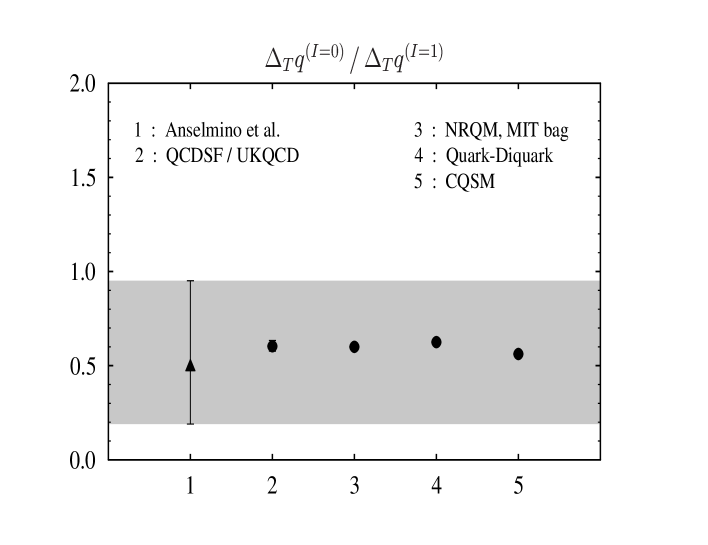
Figure 8: Comparison of empirical and theoretical tensor charge ratio $\Delta_{T}q^{(I=0)}/\Delta_{T}q^{(I=1)}$, which is scale independent.

Next, in Fig.8, a similar comparison is made for the tensor charge ratio $\Delta_{T}q^{(I-0)}/\Delta_{T}q^{(I=1)}$. Again, the prediction of the CQSM gives the smallest value among all the theoretical predictions. Within the large error-bars, however, all the theoretical predictions are consistent with the phenomenological value. We emphasize once again that the tensor charge ratio as $|\Delta_{T}d/\Delta_{T}u|$ and $\Delta_{T}q^{(I=0)}/\Delta_{T}q^{(I=1)}$ are exactly scale independent so that it offers a safe and sound basis of comparison between theoretical predictions and the empirical extractions. Further effort to reduce the uncertainties of phenomenological extraction would be highly desirable.

As a general trend, one observes that the predictions for the tensor charge ratio $\Delta_{T}q^{(I=0)}/\Delta_{T}q^{(I=1)}$ by all the low energy models as well as by the lattice QCD are not extremely far from the reference value of the SU(6) quark model, i.e. 3/5. This feature of the tensor charges should be contrasted with that of axial charges. In Fig.9, we compare the empirically known axial-charge ratio $\Delta q^{(I=0)}/\Delta q^{(I=1)}$ with the predictions of several models and with that of lattice QCD. The empirical value here is taken from the HERMES analysis of the longitudinally polarized structure functions of the deuteron and proton HERMES07 . (See also a similar analysis by COMPASS group COMPASS05 ,COMPASS07 .) One sees that fairly small empirical ratio, which is connected with the famous “nucleon spin crisis”, is reproduced only by the CQSM and the lattice QCD, while the predictions of other low energy models are more or less close to that of the SU(6) quark model, i.e. $\Delta^{(I=0)}/\Delta^{(I-1)}=3/5$, thereby largely overestimating this ratio.

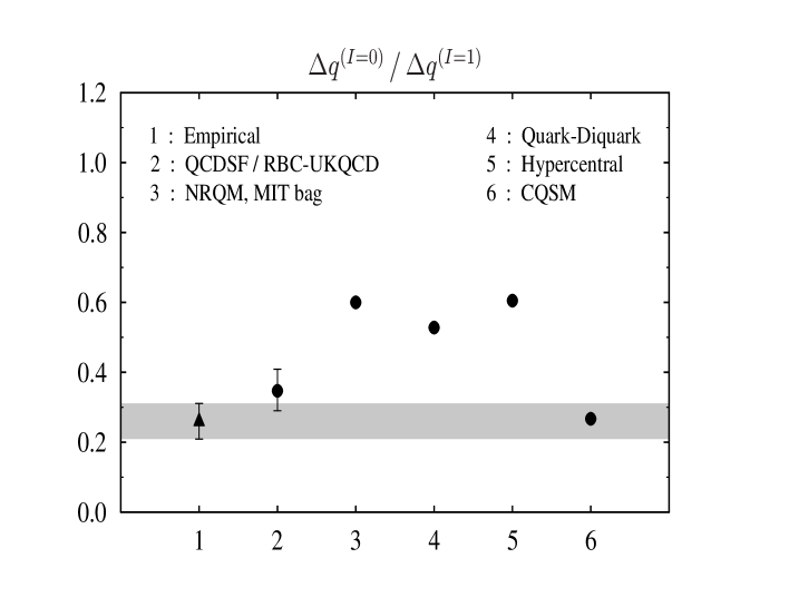
Figure 9: Comparison of empirical and theoretical axial charge ratio $\Delta q^{(I=0)}/\Delta q^{(I=1)}$, which is approximately scale independent.

In any case, as we have repeatedly emphasized, the possible difference between the axial and tensor charges of the nucleon (or more generally, the difference between the longitudinally polarized distribution functions and the transversity distribution functions of the nucleon) offers one of the key information for disentangling the internal spin structure of the nucleon. Particularly useful here, we think, is the comparison between the two ratios, i.e. $\Delta_{T}q^{(I=0)}/\Delta_{T}q^{(I=1)}$ and $\Delta q^{(I=0)}/\Delta q^{(I=1)}$. As we have emphasized, the former ratio is exactly scale independent, while the latter has only a weak scale dependence, so that it offers a safe and sound basis of comparison between theoretical predictions and empirical extractions for them. Further effort to reduce the uncertainties of the phenomenological extraction of the tensor charges is highly desirable to get more definite information on the possible difference of these two fundamental quantities. Do we expect a spin crisis also for the transverse spins, or the tensor charges ?

IV Conclusion

In summary, we have investigated the forward limit of a particular combination of chiral-odd generalized parton distributions, i.e. $G_{T}(x,0,0)\equiv\lim_{\xi\rightarrow 0,t\rightarrow 0}\,[\,H_{T}(x,\xi,t)+2\,\tilde{H}_{T}(x,\xi,t)+E_{T}(x,\xi,t)\,]$ as well as their lower moments within the framework of the chiral quark soliton model, with particular emphasis upon the transversity decomposition of the nucleon angular momentum proposed by Burkardt. We found rather strong chiral enhancement near $x\sim 0$ for both of the isoscalar and isovector GPDs, which reminds us of a similar chiral enhancement observed in the CQSM predictions for more familiar unpolarized distribution functions of isoscalar and isovector types. We have shown that the $G_{T}$ is an isoscalar-dominant quantity, while the isovector component also arises as an $1/N_{c}$ correction. In particular, from the 1st moment sum rule of $G_{T}$ and $H_{T}$, we have confirmed a isoscalar dominance of the “anomalous tensor moments” $\kappa_{T}$, which indicates that the Boer-Mulders functions for the $u$- and $d$-quarks would have roughly equal magnitude with the same sign. It should be contrasted with the probable isovector dominance of the Sivers functions, or of the anomalous magnetic moment of the nucleon. It is therefore a very important experimental challenge to determine the relative sign and the magnitudes of the $u$- and $d$-quark Boer-Mulders functions.

We have also discussed a delicate problem, which may arise when we try to compare the phenomenologically extracted tensor charges with corresponding theoretical predictions. We emphasize that the tensor charges are strongly scale dependent quantities but the ratios as $\Delta_{T}d/\Delta_{T}u$ and $\Delta_{T}q^{(I=0)}/\Delta_{T}q^{(I=1)}$ are exactly scale independent, so that these ratios are expected to provide us with a safe and convenient basis of comparison between empirically determined tensor charges of the nucleon and corresponding theoretical predictions.

Appendix A On the 1st moment of $\tilde{E}_{T}(x,0,0)$

In this appendix, we shall explicitly verify that the 1st moment of $\tilde{E}_{T}(x,0,0)$ vanishes. At the $O(\Omega^{0})$ level, only the isovector part of $\tilde{E}_{T}(x,0,0)$ survives as given by eq.(II). Its 1st moment can easily be written down as

$$\int_{-1}^{1}\,\frac{1}{2\,M_{N}}\,\,\tilde{E}_{T}^{(I=1)}(x,0,0)\,dx = -\,\frac{N_{c}}{3}\,\sum_{n\in occ}\,\langle n\,|\,\tau_{3}\,\,i\,x_{1}\,(\gamma^{1}\,\gamma_{5}-i\,\gamma^{2})\,|\,n\rangle$$ (72)

$$= -\,\frac{N_{c}}{18}\,\sum_{n\in occ}\,\langle n\,|\,\mbox{\boldmath$\tau$}\cdot(\mbox{\boldmath$x$}\times\mbox{\boldmath$\gamma$})\,|\,n\rangle.$$

Very interestingly, this expression resembles that of the $O(\Omega^{0})$ contribution to the isovector magnetic moment of the nucleon in the CQSM given as

$$\mu^{(I=1)}(\Omega^{0}) = -\,M_{N}\,\frac{N_{c}}{9}\,\sum_{n\in occ}\,\langle n\,|\,\mbox{\boldmath$\tau$}\cdot(\mbox{\boldmath$x$}\times\gamma^{0}\,\mbox{\boldmath$\gamma$})\,|\,n\rangle,$$ (73)

where use has been made of the generalized spherical symmetry of the hedgehog configuration. Incidentally, we already know that the time reversal invariance enforces the 1st moment of $\tilde{E}_{T}$ to vanish. As a consistency check of our theoretical framework, we shall verify it explicitly in the following. The formal proof in the CQSM utilizes the invariance under the $G_{5}$ transformation, which is a simultaneous operations of the standard time reversal and a flavor SU(2) rotation. In a standard representation, it is given as

$$G_{5}\ =\ \gamma^{1}\,\gamma^{2}\,\tau_{2},$$ (74)

and satisfies the following identities

$$G_{5}\,\gamma^{\mu}\,G_{5}^{-1} = \left(\gamma^{\mu}\right)^{T},\ \ \ \ \ G_{5}\,\tau_{a}\,G_{5}^{-1}\ =\ -\,\left(\tau_{a}\right)^{T},$$ (75)

$$G_{5}\,\Phi_{n}(\mbox{\boldmath$x$}) = \Phi_{n}^{*}(\mbox{\boldmath$x$}),\ \ \ \ \ G_{5}\,H\,G_{5}^{-1}\ =\ H^{T}.$$ (76)

Using these properties, it is easy to verify the relations

$$\langle n\,|\,\mbox{\boldmath$\tau$}\cdot(\mbox{\boldmath$x$}\times\mbox{\boldmath$\gamma$})\,|\,n\rangle = +\,\langle n\,|\,\mbox{\boldmath$\tau$}\cdot(\mbox{\boldmath$x$}\times\mbox{\boldmath$\gamma$})\,|\,n\rangle,$$

$$\langle n\,|\,\mbox{\boldmath$\tau$}\cdot(\mbox{\boldmath$x$}\times\gamma^{0}\,\mbox{\boldmath$\gamma$})\,|\,n\rangle = -\,\langle n\,|\,\mbox{\boldmath$\tau$}\cdot(\mbox{\boldmath$x$}\times\gamma^{0}\,\mbox{\boldmath$\gamma$})\,|\,n\rangle,$$ (77)

where use has been made of the reality of the relevant matrix elements. These relations then dictates that the 1st moment of $\tilde{E}_{T}^{(I-1)}$ must vanish identically, while $\mu^{(I=1)}$ need not, as expected. At the $O(\Omega^{1})$ level, both the isoscalar and the isovector parts of $\tilde{E}_{T}(x,0,0)$ survive at the first glance. In fact, their contribution to the 1st moments take the following forms :

$$\int_{-1}^{1}\,\frac{1}{2\,M_{N}}\,\tilde{E}_{T}^{(I=0)}(x,0,0)\,dx$$

$$=\ \frac{1}{2\,I}\,\left(\frac{N_{c}}{2}\right)\,\sum_{m\in nocc,n\in occ}\,\frac{1}{E_{m}-E_{n}}\,\langle n\,|\,(\mbox{\boldmath$x$}\times\mbox{\boldmath$\gamma$})_{3}\,|\,m\rangle\,\langle m\,|\,\tau_{3}\,|\,n\rangle,$$

$$\int_{-1}^{1}\,\frac{1}{2\,M_{N}}\,\tilde{E}_{T}^{(I=1)}(x,0,0)\,dx$$

$$=\ i\,\varepsilon_{3ac}\,\,\frac{N_{c}}{6\,I}\,\sum_{m\in nocc,n\in occ}\,\frac{1}{E_{m}-E_{n}}\,\langle n\,|\,\tau_{a}\,x_{1}\,\gamma_{2}\,|\,m\rangle\,\langle m\,|\,\tau_{c}\,|\,n\rangle.$$ (79)

However, it is not so difficult to prove that both of the above expressions vanishes owing to the symmetry under the $G_{5}$ transformation. Since the SU(2) isospin symmetry is naturally respected in our effective theory, this just reconfirms the general statement that the 1st moments $\tilde{E}_{T}^{(I=0,1)}$ vanish by time reversal invariance.

References

- (1) D. Mueller, D. Robaschik, B. Geyer, F.M. Dittes, and J. Horejsi, Fortsch. Phys. 42, 101 (1994).
- (2) F.M. Dittes, D. Mueller, D. Robaschik, B. Geyer, and J. Horejsi, Phys. Lett. B209, 325 (1988).
- (3) X. Ji. J. Phys. G 24, 1181 (1998).
- (4) K. Goeke, M.V. Polyakov, and M. Vanderhaeghen, Prog. Part. Nucl. Phys. 47, 401 (2001).
- (5) M. Diehl, Phys. Rep. 388, 41 (2003).
- (6) A.V. Belitsky and A.V. Radyushkin, Phys. Rep. 418, 1 (2005).
- (7) P. Hoodbhoy and X. Ji, Phys. Rev. D 58, 054006 (1998).
- (8) M. Diehl, Eur. Phys. J. C19, 485 (2001).
- (9) F. Ellinghaus, W.-D. Nowak, and A.V. Vinnikov, Eur. Phys. J. C46, 729 (2006).
- (10) F. Ellinghaus, arXiv:0710.5768 (2007).
- (11) Z. Ye, hep-ex/0606061 (2006).
- (12) JLab Hall A Collaboration, M. Mazous et al., Phys. Rev. Lett. 99, 242501 (2007).
- (13) X. Ji, Phys. Rev. Lett. 78, 610 (1997).
- (14) P. Hoodbhoy, X. Ji, and W. Lu, Phys. Rev. D 59, 014013 (1999).
- (15) X. Ji, J. Tang, and P. Hoodbhoy, Phys. Rev. Lett. 76, 740 (1996).
- (16) D.Yu Ivanov, B. Pire, L. Szymanowski, and O.V. Teryaev, Phys. Lett. B550, 65 (2002).
- (17) D.Yu Ivanov, B. Pire, L. Szymanowski, and O.V. Teryaev, Phys. Part. Nucl. 35, S67 (2004).
- (18) M. Anselmino, M. Boglione, U. D’Alesio, A. Kotzinian, F. Murgia, A. Prokudin, and C. Türk, Phys. Rev. D 75, 054032 (2007).
- (19) A. Anselmino, M. Boglione, U. D’Alesio, E. Leader, S. Melis, and F. Murgia, arXiv:0809.3743 [hep-ph] (2008).
- (20) M. Burkardt, Phys. Rev. D 72, 094020 (2005).
- (21) M. Burkardt, Phys. Lett. B639, 462 (2006).
- (22) D. Boer and P.J. Mulders, Phys. Rev. D 57, 5780 (1998).
- (23) D.W. Sivers, Phys. Rev. D 43, 261 (1991).
- (24) M. Burkardt, Nucl. Phys. A735, 185 (2004) ; Phys. Rev. D 69, 074032 (2004).
- (25) M. Burkardt, Phys. Rev. D 69, 057501 (2004).
- (26) J.M. Olness, Phys. Rev. D 47 (1993) 2136
- (27) H. He and X, Ji, Phys. Rev. D bf 52 (1995) 2960.
- (28) H.-C. Kim, M.V. Polyakov, and K. Goeke, Phys. Lett. B387 (1996) 577.
- (29) H. He and X. Ji, Phys. Rev. D 54 (1996) 6897.
- (30) I. Schmidt and J. Soffer, Phys. Lett. B407 (1997) 331.
- (31) L. Gamberg, H. Reinhardt, and H. Weigel, Phys. Rev. D 58 (1998) 054014.
- (32) M. Wakamatsu and T. Kubota, Phys. Rev. D 60 (1999) 034020
- (33) P. Schweitzer, D. Urbano, M.V. Polyakov, C. Weiss, P.V. Pobylitsa, and K. Goeke, Phys. Rev. D 64 034013 (2001).
- (34) M. Wakamatsu, Phys. Lett. B509, 59 (2001).
- (35) A.V. Efremov, O.V. Teryaev, and P. Zavada, Phys. Rev. D 70 (2004) 054018.
- (36) M. Wakamatsu, Phys. Lett. B653, 398 (2007).
- (37) I.C. Cloët, W. Benz, and A.W. Thomas, Phys. Lett. B659, 214 (2008).
- (38) S. Aoki, M. Doi, T. Hatsuda, and Y. Kuramashi, Phys. Rev. D 56 (1997) 433.
- (39) M. Göckeler, Ph. Hägler, R. Horsley, D. Pleiter, P.E.L. Rakow, A. Scäfer, G. Shierholz, and J.M. Zanotti, Phys. Lett. B627, 113 (2005).
- (40) B. Pasquini, M. Pincetti, and S. Boffi, Phys. Rev. D 72 094029 (2005).
- (41) M. Pincetti, B. Pasquini, and S. Boffi, Czech. J. Phys. 56, F229 (2006).
- (42) S. Boffi and B. Pasquini, Riv. Nuovo Cim. 30, 387 (2007).
- (43) H. Dahiya and A.Mukherjee, Phys. Rev. D 77, 045032 (2008).
- (44) S. Scopetta, Phys. Rev. D 72, 117502 (2005).
- (45) V.Yu. Petrov, P.V. Pobylitsa, M.V. Polyakov, I. Böring, K. Goeke, and C. Weiss, Phys. Rev. D 57, 4325 (1998).
- (46) J. Ossmann, M.V. Polyakov, P. Schweitzer, D. Urbano, and K. Goeke. Phys. Rev. D 71, 034011 (2005).
- (47) M. Wakamatsu and H. Tsujimoto, Phys. Rev. D 71, 074001 (2005).
- (48) M. Wakamatsu and Y. Nakakoji, Phys. Rev. D 74, 054006 (2006).
- (49) M. Wakamatsu and Y. Nakakoji, Phys. Rev. D 77, 074011 (2008)
- (50) K. Goeke, J. Grabis, J. Ossmann, M.V. Polyakov, P. Schweitzer, A. Silve, and D. Urbano, Phys. Rev. C 75, 055207 (2007).
- (51) K. Goeke, J. Grabis, J. Ossmann, M.V. Polyakov, P. Schweitzer, A. Silve, and D. Urbano, Phys. Rev. D 75, 094021 (2007).
- (52) D.I. Diakonov, V.Yu. Petrov, and P.V. Pobylitsa, Nucl. Phys. B306, 809 (1988).
- (53) M. Wakamatsu and H. Yoshiki, Nucl. Phys. A524, 561 (1991).
- (54) D.I. Diakonov, V.Yu. Petrov, P.V. Pobylitsa, M.V. Polyakov, and C. Weiss, Nucl. Phys. B480, 341 (1996).
- (55) D.I. Diakonov, V.Yu. Petrov, P.V. Pobylitsa, M.V. Polyakov, and C. Weiss, Phys. Rev. D56, 4069 (1997).
- (56) H. Weigel, L. Gamberg, H. Reinhardt, Mod. Phys. Lett. A11, 3021 (1996).
- (57) H. Weigel, L. Gamberg, and H. Reinhardt, Phys. Lett. B399, 287 (1997).
- (58) M. Wakamatsu and T. Kubota, Phys. Rev. D 57. 5755 (1998).
- (59) P.V. Pobylitsa, M.V. Polyakov, K. Goeke, T. Watabe, and C. Weiss, Phys. Rev. D 59, 034024 (1999).
- (60) M. Wakamatsu, Phys. Rev. D 67, 034005 (2003).
- (61) M. Wakamatsu, Phys. Rev. D 67, 034006 (2003).
- (62) M. Wakamatsu and T. Watabe, Phys. Lett. B312, 184 (1993).
- (63) Chr.V. Christov, A. Blotz, K. Goeke, P. Pobylitsa, V.Yu. Petrov, M. Wakamatsu, and T. Watabe, Phys. Lett. B325, 467 (1994).
- (64) M. Wakamatsu, Prog. Theor. Phys. 95, 143 (1996).
- (65) NMC Collaboration, P. Amaudruz et al., Phys. Rev. Lett. 66, 2712 (1991).
- (66) P.V. Pobylitsa, in “Large QCD 2004”, eds. J. Goity et al. (World Scientific, 2005), p.302.
- (67) M. Glück, E. Reya, and A. Vogt, Z. Phys. C67, 433 (1995).
- (68) S. Kumano and M. Miyama, Phys. Rev. D 56, R2504 (1997).
- (69) A. Hayashigaki, Y. Kanazawa, and Y. Koike, Phys. Rev. D 56, 7350 (1997).
- (70) W. Vogelsang, Phys. Rev. D 57, 1886 (1998).
- (71) HERMES Collaboration, A. Airapetian et al., Phys. Rev. D 75, 012007 (2007).
- (72) COMPASS Collaboration, E.S. Ageev et al., Phys. Lett. B612, 154 (2005).
- (73) COMPASS Collaboration, V.Yu. Alexakhin et al., Phys. Lett. B647, 8 (2007).
- (74) G. Altarelli and c.G. Ross, Phys. Lett. B212, 391 (1988).
- (75) D. Carlitz, J.C. Collins, and H.A. Müller, Phys. Lett. B214, 229 (1988).
- (76) A.V. Efremov and O.V. Teryaev, JINR Research Report No. E2-88, 287 (1988).