The noise spectra of a biased quantum dot

Abstract

The noise spectra associated with correlations of the current through a single level quantum dot, and with the charge fluctuations on the dot, are calculated for a finite bias voltage. The results turn out to be sensitive to the asymmetry of the dot’s coupling to the two leads. At zero temperature, both spectra exhibit two or four steps (as a function of the frequency), depending on whether the resonant level lies outside or within the range between the chemical potentials on the two leads. In addition, the low frequency shot-noise exhibits dips in the charge noise and dips, peaks, and discontinuities in the derivative of the current noise. In spite of some smearing, several of these features persist at finite temperatures, where a dip can also turn into a peak.

I Introduction

Ten years ago, Landauer coined the phrase “the noise is the signal”.LANDU Indeed, the noise spectrum of electronic transport through mesoscopic systems provides invaluable information on the physics which governs this transport.book ; BB The noise spectrum is given by the Fourier transform of the current-current correlation. The un-symmetrized noise spectrum is defined as book

$$C_{\alpha\alpha^{\prime}}(\omega)=\int_{-\infty}^{\infty}dte^{-i\omega t}\langle\delta\hat{I}_{\alpha}(t)\delta\hat{I}_{\alpha^{\prime}}(0)\rangle\ ,$$ (1)

where $\alpha$ and $\alpha^{\prime}$ mark the leads, which carry the current from the electron reservoirs to the mesoscopic system. In Eq. (1), $\delta\hat{I}_{\alpha}\equiv\hat{I}_{\alpha}-\langle\hat{I}_{\alpha}\rangle$, where $\hat{I}_{\alpha}$ is the current operator in lead $\alpha$, and the average (denoted by $\langle\ldots\rangle$) is taken over the states of the reservoirs (see below). At finite frequencies, this quantity is very sensitive to the locations where those currents are monitored. When $\alpha=\alpha^{\prime}$, Eq. (1) gives the auto-correlation function, while for $\alpha\neq\alpha^{\prime}$ it yields the cross-correlation one. Clearly, $C_{\alpha\alpha^{\prime}}(\omega)=C_{\alpha^{\prime}\alpha}^{\ast}(\omega)$, and consequently the auto-correlation function is real. Some papers prefer to analyze the symmetrized noise spectrum, defined as $[C_{\alpha\alpha^{\prime}}(\omega)+C_{\alpha^{\prime}\alpha}(-\omega)]/2$. However, as we discuss below, this spectrum may miss some important features. Particular measurements require the calculation of different combinations of the $C_{\alpha\alpha^{\prime}}$’s.

In this article we calculate the various current correlations, $C_{\alpha\alpha^{\prime}}(\omega)$, for the simplest mesoscopic system, i.e. a single level quantum dot connected to two electron reservoirs via leads $L$ and $R$. The latter are kept at different chemical potentials, $\mu_{L}$ and $\mu_{R}$. The potential difference,

$$V=(\mu_{L}-\mu_{R})/e\ ,$$ (2)

represents the bias voltage applied to the dot. It is convenient to measure energies relative to the common Fermi energy, $(\mu_{L}+\mu_{R})/2$. Setting this energy to zero, we have $\mu_{L}=-\mu_{R}=eV/2$. Having two leads, one can consider two auto-correlation functions, $C_{LL}(\omega)$ and $C_{RR}(\omega)$, and two cross-correlation functions, $C_{LR}(\omega)$ and $C_{RL}(\omega)$.

The operator of the net current going through the dot is given by

$$\hat{I}=(\hat{I}_{L}-\hat{I}_{R})/2\ .$$ (3)

With a finite bias voltage, $\langle\hat{I}\rangle$ is not necessarily zero. The noise associated with $\hat{I}$ is then given by

$$C^{(-)}(\omega)=\frac{1}{4}\Bigl{(}C_{LL}(\omega)+C_{RR}(\omega)-C_{LR}(\omega)-C_{RL}(\omega)\Bigr{)}\ .$$ (4)

Since $C_{LR}(\omega)=C^{\ast}_{RL}(\omega)$, $C^{(-)}(\omega)$ is real. Alternatively, one could also consider the difference between the currents flowing into the dot from the two leads,

$$\Delta\hat{I}=(\hat{I}_{L}+\hat{I}_{R})/2\ ,$$ (5)

for which $\langle\Delta\hat{I}\rangle=0$.BB The fluctuations in this difference account for the fluctuations in the net charge accumulating on the dot. The noise associated with this charge is given by

$$C^{(+)}(\omega)=\frac{1}{4}\Bigl{(}C_{LL}(\omega)+C_{RR}(\omega)+C_{LR}(\omega)+C_{RL}(\omega)\Bigr{)}\ .$$ (6)

Earlier theoretical papers considered various aspects of noise correlations in mesoscopic systems. Some of these studies analyzed only the low frequency limit of the spectrum, which reduces to the Johnson-Nyquist noise at equilibrium (i.e. at zero bias voltage) and to the shot noise at a finite bias. Specifically, Chen and TingCHEN studied the un-symmetrized noise associated with the net terminal current [our Eq. (3)], and found a Lorentzian peak around zero frequency for a bias which is larger than the resonance level width. AverinAVERIN then studied the shot noise for any value of the bias, but considered only the symmetrized noise at the zero frequency limit. Engel and LossENGEL extended these results to finite frequencies and to the un-symmetrized noise, but considered only the auto-correlation function. They found steps at particular frequencies. For the two level dot they also found a dip in the auto-correlation noise around zero frequency, which they attributed to “the charging effect of the dot”.

Recently, two of us participated in a detailed analysis of $C^{(-)}(\omega)$ in the limit of zero temperature and zero bias.EWIGA Ignoring interactions and capacitance effects, which might add correlations among the currents at relatively high frequencies,BB ; BUT1 ; BUT2 it is convenient to use the single electron scattering formalism for obtaining explicit expressions for the noise spectrum.but0 ; lev Similar to Ref.  ENGEL, , Ref.  EWIGA, found that the current noise spectrum $C^{(-)}(\omega)$ has a step structure as a function of the frequency, with the step edges located roughly at energies corresponding to the resonances of the quantum dot. It was consequently suggested that the noise spectrum can be used to probe the resonance levels of the dot. For the two level quantum dot, Ref.  EWIGA, also found dips in the noise spectrum, which appeared when the Fermi energy was between the two levels and deepened upon increasing the asymmetry of the coupling of the dot to the leads.

The present paper generalizes Ref.  EWIGA, , by introducing a finite bias and and a finite temperature, and by considering also the charge noise. In particular, we discuss the interesting dependence of the various spectra on the spatial asymmetry, denoted by

$$a=\frac{\Gamma_{R}-\Gamma_{L}}{\Gamma_{R}+\Gamma_{L}}\ ,\ \ -1\leq a\leq 1\ ,$$ (7)

where $\Gamma_{L}$ ($\Gamma_{R}$) denote the broadening of the resonance on the dot due to its coupling with the left (right) lead. We find that the single step appearing in $C^{(\pm)}(\omega)$ in the absence of the bias EWIGA splits in the presence of $V$ into two steps when the resonance energy $\epsilon_{d}$ is not between the two chemical potentials ($|\epsilon_{d}|>|eV/2|$) and into four steps when it is within that range. In addition, $C^{(+)}(\omega)$ vanishes at $\omega=0$, exhibiting a dip in the shot noise around $\omega=0$. For $|\epsilon_{d}|<|eV/2|$ and for $0<|a|<1$ there also appears a peak in $C^{(-)}(\omega)$ at $\omega=0$. At zero temperature and close to $|eV/2|=|\epsilon_{d}|$ we also find a discontinuity in the slope of $C^{(-)}(\omega)$. Many of these features are smeared as the temperature $T$ increases. However, both $C^{(+)}(\omega)$ and $C^{(-)}(\omega)$ still exhibit dips and peaks near $\omega=0$ even at $T>0$.

Our paper is divided into two main sections. In Sec. II we discuss some general properties of the noise spectra, present a short review of the scattering matrix formalism, and from that derive the various noise spectra for a single level quantum dot. In the following section we analyze both $C^{(+)}(\omega)$ and $C^{(-)}(\omega)$, with and without a bias voltage and at both zero and non-zero temperatures. The last section summarizes our results.

II The noise spectra

II.1 General relations

We begin our discussion by describing several general properties of the noise spectrum (which also hold for interacting systems). The physical meaning of the auto-correlation function is revealed upon re-writing it in the form GAVISH2

$$C_{\alpha\alpha}(\omega)=2\pi\sum_{i,f}P_{i}|\langle i|\delta\hat{I}_{\alpha}|f\rangle|^{2}\delta(E_{i}-E_{f}-\omega)\ .$$ (8)

Here, $|i\rangle$ and $|f\rangle$ are the initial and final states of the whole system (the dot and its leads), with the corresponding energies $E_{i}$ and $E_{f}$. In Eq. (8), $P_{i}$ is the probability for the system to be in the initial state $|i\rangle$. It is now seen that the auto-correlation is the rate (as given by the Fermi golden-rule) by which the system absorbs energy from a monochromatic electromagnetic field of frequency $\omega$. The symmetrized noise spectrum mixes absorption and emission, and thus loses the separation between the two.

At zero frequency, $\omega=0$, the auto-correlation and the cross-correlation are related to one another. This follows from charge conservation.AVI The equation of motion for $\delta\hat{n}(t)$, the fluctuation of the occupation operator on the dot, is given by

$$e\frac{d\delta\hat{n}(t)}{dt}=\delta\hat{I}_{L}(t)+\delta\hat{I}_{R}(t)\ .$$ (9)

[Note that in our convention, the currents flowing in the left (right) lead, $\hat{I}_{L}$ ($\hat{I}_{R}$), are directed towards the dot.] Equation (9) implies that

$$C_{L\alpha}(0)+C_{R\alpha}(0)=e\int_{-\infty}^{\infty}dt\langle\frac{d\delta\hat{n}(t)}{dt}\delta\hat{I}_{\alpha}(0)\rangle$$

$$=e\lim_{\tau\rightarrow\infty}\langle\delta\hat{n}(\tau)\delta\hat{I}_{\alpha}(0)-\delta\hat{n}(-\tau)\delta\hat{I}_{\alpha}(0)\rangle\ .$$ (10)

At steady-state, assuming no long-term memory, we have $\lim_{\tau\rightarrow\pm\infty}\langle\delta\hat{n}(\tau)\delta\hat{I}_{\alpha}(0)\rangle=\langle\delta\hat{n}\rangle\langle\hat{I}_{\alpha}\rangle$, and therefore $C_{L\alpha}(0)+C_{R\alpha}(0)=0$.AVI As a result,

$$C_{LL}(0)=-C_{RL}(0)\ ,\ \ C_{RR}(0)=-C_{LR}(0)\ .$$ (11)

Moreover, since $C_{LL}(0)$ and $C_{RR}(0)$ are real and positive [see Eq. (8)], it follows that the zero-frequency cross-correlations are real as well, but negative. Since the cross-correlations are real, one has $C_{LR}(0)=C_{RL}(0)$, and therefore

$$C_{LL}(0)=C_{RR}(0)=-C_{LR}(0)=-C_{RL}(0)\ .$$ (12)

In particular, this implies that $C^{(+)}(0)=0$ and $C^{(-)}(0)=C_{LL}(0)$. At zero bias, those are just the Nyquist-Johnson relations, $C_{LL}(0)=C_{RR}(0)=-C_{LR}(0)=-C_{RL}(0)=k_{\rm B}TG(0)$, where $G(0)$ is the dc conductance of the dot.

II.2 The noise spectrum in the scattering formalism

When electron-electron interactions are ignored, one may use the (single-particle) scattering matrix of the dot to obtain an expression for the noise spectrum in terms of the scattering matrix elements. This has been accomplished in Refs.   BUT1, and   BUT2, .

In the scattering formalism, one expresses the current operator $\hat{I}$ in terms of creation [$\hat{a}^{\dagger}_{\alpha}(E)$] and annihilation [$\hat{a}_{\alpha}(E)$] operators of the electrons in the reservoir connected to terminal $\alpha$. These operators are normalized such that

$$\langle\hat{a}^{\dagger}_{\alpha}(E)\hat{a}_{\alpha^{\prime}}(E^{\prime})\rangle=\delta_{\alpha\alpha^{\prime}}\delta(E-E^{\prime})f_{\alpha}(E)\ ,$$ (13)

where $f_{\alpha}(E)\equiv[\exp(E-\mu_{\alpha})/k_{\rm B}T+1]^{-1}$ is the Fermi distribution in reservoir $\alpha$ which is held at the chemical potential $\mu_{\alpha}$. The explicit form for the current operator (using units in which $\hbar=1$) is but0

$$\hat{I}_{\alpha}(t) =\frac{e}{2\pi}\int_{-\infty}^{\infty}dE\int_{-\infty}^{\infty}dE^{\prime}e^{i(E-E^{\prime})t}$$

$$\times\sum_{\gamma\gamma^{\prime}}A_{\gamma\gamma^{\prime}}(\alpha,E,E^{\prime})\hat{a}^{\dagger}_{\gamma}(E)\hat{a}_{\gamma^{\prime}}(E^{\prime})\ ,$$ (14)

with

$$A_{\gamma\gamma^{\prime}}(\alpha,E,E^{\prime})=\delta_{\gamma\gamma^{\prime}}\delta_{\alpha\gamma}-S^{\ast}_{\alpha\gamma}(E)S_{\alpha\gamma^{\prime}}(E^{\prime})\ ,$$ (15)

where Greek letters denote the lead indices and $S_{\alpha\gamma}$ are the elements of the scattering matrix characterizing the dot.

Inserting the expression for the current operator, Eq. (14), into Eq. (1) and calculating the averages according to Eq. (13), we find

$$C_{\alpha\alpha^{\prime}}(\omega) =\frac{e^{2}}{2\pi}\int_{-\infty}^{\infty}dE\sum_{\gamma\gamma^{\prime}}F^{\alpha\alpha^{\prime}}_{\gamma\gamma^{\prime}}(E,\omega)$$

$$\times f_{\gamma}(E+\omega)(1-f_{\gamma^{\prime}}(E))\ ,$$ (16)

where

$$F^{\alpha\alpha^{\prime}}_{\gamma\gamma^{\prime}} (E,\omega)\equiv A_{\gamma\gamma^{\prime}}(\alpha,E+\omega,E)A_{\gamma^{\prime}\gamma}(\alpha^{\prime},E,E+\omega)$$

$$=A_{\gamma\gamma^{\prime}}(\alpha,E+\omega,E)A^{\ast}_{\gamma\gamma^{\prime}}(\alpha^{\prime},E+\omega,E)\ .$$ (17)

It is straightforward to verify, using the unitarity of the scattering matrix, that the zero-frequency relations (12) are obeyed by the form (II.2). Another limit of Eq. (II.2) is obtained upon neglecting the energy dependence of the scattering matrix elements. Then (at zero temperature and for $\omega>0$) one retrieves the well-known result book $C_{LL}(\omega)=(e^{2}/2\pi){\cal T}(1-{\cal T})(eV-\omega)\Theta(eV-\omega)$, where ${\cal T}$ is the transmission of the dot.

We next discuss the correlation functions $C^{(\pm)}(\omega)$, Eqs. (4) and (6). Upon inserting Eqs. (15) and (II.2) into Eqs. (4) and (6) we obtain

$$C^{(\pm)}(\omega) =\frac{e^{2}}{8\pi}\int_{-\infty}^{\infty}dE\sum_{\gamma\gamma^{\prime}}F^{(\pm)}_{\gamma\gamma^{\prime}}(E,\omega)$$

$$\times f_{\gamma}(E+\omega)(1-f_{\gamma^{\prime}}(E)),$$ (18)

where

$$F^{(\pm)}_{LL}(E,\omega)=\Big{|}1-S^{\ast}_{LL}(E+\omega)S_{LL}(E)$$

$$\ \ \ \ \ \ \ \ \ \mp S^{\ast}_{RL}(E+\omega)S_{RL}(E)\Big{|}^{2}\ ,$$

$$F^{(\pm)}_{LR}(E,\omega)=\Big{|}S^{\ast}_{LL}(E+\omega)S_{LR}(E)$$

$$\ \ \ \ \ \ \ \ \ \pm S^{\ast}_{RL}(E+\omega)S_{RR}(E)\Big{|}^{2}\ .$$ (19)

The other correlations, $F^{(\pm)}_{RR}(E,\omega)$ and $F^{(\pm)}_{RL}(E,\omega)$, are obtained from these expressions upon interchanging $L\leftrightarrow R$. In this way we divide the correlation functions $C^{(\pm)}(\omega)$ according to the separate contributions of the various processes: $F^{(\pm)}_{LL}(E,\omega)$ and $F^{(\pm)}_{RR}(E,\omega)$ describe intra-lead transitions of the electron, while $F^{(\pm)}_{LR}(E,\omega)$ and $F^{(\pm)}_{RL}(E,\omega)$ give the contributions of the inter-lead processes. The actual contribution of each process to $C^{(\pm)}(\omega)$ is determined by the relevant product of the Fermi functions. In particular, at zero temperature ($T=0$), this product vanishes everywhere except on a finite segment of the energy axis. Finite temperatures broaden and smear the limits of this section, while the application of the bias voltage may shift it along the energy axis or change its length.

II.3 A single level dot

In our simple configuration, the dot is represented by a single energy level denoted $\epsilon_{d}$. As mentioned, we denote the broadening due to the coupling with the left lead by $\Gamma_{L}$, and that due to the coupling with the right one by $\Gamma_{R}$, such that the total width of the energy level on the dot is

$$\Gamma=\Gamma_{L}+\Gamma_{R}\ .$$ (20)

In this model the scattering matrix takes the form

$$S(E) =\left[\begin{array}[]{cc}S_{LL}(E)&S_{LR}(E)\\ S_{RL}(E)&S_{RR}(E)\end{array}\right]$$ (23)

$$=-1+ig(E)\left[\begin{array}[]{cc}\Gamma_{L}&\sqrt{\Gamma_{L}\Gamma_{R}}\\ \sqrt{\Gamma_{L}\Gamma_{R}}&\Gamma_{R}\end{array}\right]\ ,$$ (26)

where $g(E)$ is the Breit-Wigner resonance formed by the dot,

$$g(E)=\frac{1}{E-\epsilon_{d}+i\Gamma/2}\ .$$ (27)

(Assuming the scattering to take place at about the Fermi energy, we have discarded the energy dependence of the resonance partial widths.)

Since the dot forms a Breit-Wigner resonance, it is useful to express the functions $F^{(\pm)}_{\alpha\alpha^{\prime}}(E,\omega)$, Eq. (II.2), in terms of the resonance phase $\delta(E)$, defined by NG

$${\rm cot}\delta(E)=\frac{2}{\Gamma}(\epsilon_{d}-E)\ ,$$ (28)

such that $g(E)$, Eq. (27), becomes

$$g(E)=-i\frac{2}{\Gamma}\sin\delta(E)e^{-i\delta(E)}\ .$$ (29)

Clearly, $|g(E)|^{2}$ is peaked around $E=\epsilon_{d}$, and the phase $\delta(E)$ changes from 0 to $\pi$ within a range of width $\Gamma$ around this resonance.

Using the identities

$$g(E)\pm g^{\ast}(E+\omega)=a_{\pm}g(E)g^{\ast}(E+\omega),$$ (30)

where

$$a_{-} =\omega-i\Gamma=\frac{\Gamma\sin[\delta(E+\omega)-\delta(E)]}{2\sin\delta(E)\sin\delta(E+\omega)}-i\Gamma,$$

$$a_{+} =2(E-\epsilon_{d})+\omega=-\frac{\Gamma}{2}[\cot\delta(E)+\cot\delta(E+\omega)]$$

$$=-\frac{\Gamma\sin[\delta(E+\omega)+\delta(E)]}{2\sin\delta(E)\sin\delta(E+\omega)}\ ,$$ (31)

we find

$$F^{(+)}_{\gamma\gamma^{\prime}}(E,\omega) =\Gamma_{\gamma}\Gamma_{\gamma^{\prime}}|g(E)g(E+\omega)|^{2}\omega^{2}$$

$$=\frac{16\Gamma_{\gamma}\Gamma_{\gamma^{\prime}}}{\Gamma^{4}}\sin^{2}\delta(E)\sin^{2}\delta(E+\omega)\omega^{2}$$

$$=\frac{4\Gamma_{\gamma}\Gamma_{\gamma^{\prime}}}{\Gamma^{2}}\sin^{2}[\delta(E+\omega)-\delta(E)]\$$ (32)

and

$$F^{(-)}_{LR}(E,\omega) =F^{(+)}_{LR}+\Gamma_{L}\Gamma_{R}[(\Gamma_{L}-\Gamma_{R})^{2}+4(E-\epsilon_{d})(E-\epsilon_{d}+\omega)]|g(E)g(E+\omega)|^{2}$$

$$=\frac{16\Gamma_{L}\Gamma_{R}}{\Gamma^{4}}\Bigl{(}(\Gamma_{L}-\Gamma_{R})^{2}\sin^{2}\delta(E)\sin^{2}\delta(E+\omega)+\frac{\Gamma^{2}}{4}\sin^{2}\bigl{[}\delta(E+\omega)+\delta(E)\bigr{]}\Bigr{)}$$

$$F^{(-)}_{LL}(E,\omega) =F^{(+)}_{LL}+4\Gamma_{L}^{2}\Gamma_{R}^{2}|g(E)g(E+\omega)|^{2}=\frac{16\Gamma_{L}^{2}}{\Gamma^{4}}(4\Gamma_{R}^{2}+\omega^{2})\sin^{2}\delta(E)\sin^{2}\delta(E+\omega)\ .$$ (33)

Hence, each of the integrands appearing in Eq. (II.2) includes two resonances, around $E\simeq\epsilon_{d}$, and around $E+\omega\simeq\epsilon_{d}$. These resonances determine the dependence of the noise spectrum on the frequency. In the next section we study this dependence, allowing for a possible asymmetry between the left and right couplings, Eq. (7).

For maximal asymmetry, $|a|=1$, i.e. when one of the two leads is decoupled from the dot, we have $\Gamma_{L}\Gamma_{R}=0$, and therefore the inter-lead correlations vanish. In this case we have $C^{(+)}(\omega)=C^{(-)}(\omega)$.

Another general feature of Eq. (II.2) is that $C^{(\pm)}(\omega)$ is invariant under the simultaneous sign change of $V$ and of the asymmetry $a$. Therefore, we present below only results for $V>0$. In addition, the noise is also symmetric under the simultaneous sign change of $\epsilon_{d}$ and of the asymmetry parameter $a$, and therefore we present results only for $\epsilon_{d}<0$, i.e. when the localized level on the dot is placed below the common Fermi energy of the reservoirs.

As seen from Eq. (32), the functional form of the charge noise $C^{(+)}(\omega)$ is much simpler than those for the other spectra. Therefore, we start our presentations below with a discussion of $C^{(+)}(\omega)$. It also turns out to be useful to discuss the cross-correlation noise,

$$C^{(\times)}(\omega)\equiv C^{(+)}(\omega)-C^{(-)}(\omega)=[C_{LR}(\omega)+C_{RL}(\omega)]/2.$$ (34)

As we shall see below, $C^{(\times)}(\omega)$ is usually small, and it has interesting structure only in the shot-noise regime near $\omega=0$, where we find differences between $C^{(+)}(\omega)$ and $C^{(-)}(\omega)$.

III Results

III.1 The unbiased dot

The unbiased noise $C^{(-)}(\omega)$ has been treated in Ref.  EWIGA, for $T=0$. Here we extend these results also to $C^{(+)}(\omega)$ and to finite $T$. When the potential (2) vanishes, the two Fermi distributions become identical, and Eq. (II.2) becomes

$$\frac{8\pi}{e^{2}}C^{(\pm)}(\omega) =\int^{\infty}_{-\infty}dEf(E+\omega)[1-f(E)]$$

$$\times\sum_{\gamma\gamma^{\prime}}F^{(\pm)}_{\gamma\gamma^{\prime}}(E,\omega)\ .$$ (35)

In particular, Eq. (32) now implies that

$$\frac{2\pi}{e^{2}}C^{(+)}(\omega)=\int^{\infty}_{-\infty}dEf(E+\omega)[1-f(E)]$$

$$\times\sin^{2}[\delta(E)-\delta(E+\omega)]\ ,$$ (36)

independent of the asymmetry $a$.

Consider first $T=0$. In this case, the integration is over $0<E<-\omega$, and all the noise functions vanish for $\omega>0$. The phase $\delta(E)$ [Eq. (28)] increases abruptly from 0 to $\pi$ as $E$ crosses the resonance at $E\sim\epsilon_{d}$. For $\epsilon_{d}<0$, this resonance is out of the integration range, so that $\delta(E)$ does not vary much within this range. Similarly, $\delta(E+\omega)$ changes abruptly near $E\sim\epsilon_{d}-\omega$. This resonance enters the range of integration when $\omega$ goes below $\epsilon_{d}$. Using the relation $2\sin^{2}\delta dE=\Gamma d\delta$, we conclude that the integral over the resonance yields $\Gamma\pi/2$, ending up with a step $\Gamma$ in $4C^{(+)}/e^{2}$. This step agrees with the calculations of $C_{LL}$ in Ref.  ENGEL, . In fact, the variation of $4C^{(+)}(\omega)/e^{2}$ follows that of $\Gamma\delta(\omega)/\pi$. EWIGA Indeed, this step is exhibited by the full calculation of the integral, shown by the full line in Fig. 1. A similar argument applies when $\epsilon_{d}>0$, when the step arises due to the resonance at $E\sim\epsilon_{d}$. Finite temperature smears the boundaries of the integration, and thus smears the step, extending its tail to $\omega>0$, see Fig. 1. However, as stated following Eq. (12), we must have $C^{(+)}(0)=0$. For small $|\omega|$, the second line in Eq. (32) implies that

$$\frac{2\pi}{e^{2}}C^{(+)}(\omega)\approx\frac{4\omega^{2}}{\Gamma^{2}}\int^{\infty}_{-\infty}dEf(E)[1-f(E)]\sin^{4}\delta(E)\ .$$ (37)

Thus, $C^{(+)}(\omega)$ has a parabolic-like dip around $\omega=0$, as can indeed be seen in Fig. 1. At low temperatures we can replace $f(E)[1-f(E)]/(k_{B}T)$ by the Dirac delta function, and then we find $(4\pi/e^{2})C^{(+)}(\omega)\approx 8(\omega^{2}/\Gamma)^{2}k_{B}T\sin^{4}\delta(0)$. Thus, the parabola broadens with decreasing $T$, and vanishes at $T=0$.

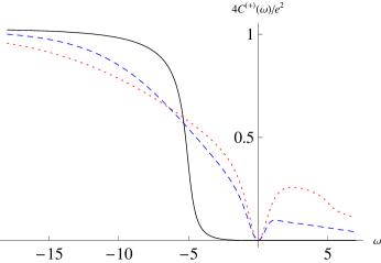
Figure 1: (Color online) The noise spectrum $C^{(+)}(\omega)$ for $V=0$. Here $\epsilon_{d}=-5$ (energies and noise are measured in units of $\Gamma$). The three curves correspond to $k_{B}T=0$ (black continuous line), $k_{B}T=3$ (blue dashed line) and $k_{B}T=5$ (red dotted line).

At maximal asymmetry, $|a|=1$, we saw that $C^{(-)}(\omega)=C^{(+)}(\omega)$. As seen from Eqs. (33) and (34), the difference $C^{(\times)}(\omega)$ involves $\Gamma_{L}\Gamma_{R}=\Gamma^{2}(1-a^{2})/4$, and therefore it does not depend on the sign of $a$, and it increases as $|a|$ decreases from $|a|=1$ to $a=0$. This difference involves an integration over the product $|g(E)g(E+\omega)|^{2}$, which is small everywhere, unless the two resonances overlap. Therefore, the cross-correlation $C^{(\times)}(\omega)$ can be relatively large only for $|\omega|\leq 2\Gamma$. Figure 2 shows $C^{(-)}(\omega)$ and $C^{(\times)}(\omega)$ for $V=0$, $T=0$ and several values of $|a|$. Indeed, $C^{(\times)}(\omega)$ has a small negative peak at $\omega\simeq\epsilon_{d}$, with the largest magnitude for $a=0$. The cross-correlation function $C^{(\times)}(\omega)$ then vanishes at some negative frequency, and reaches a small positive plateau for large negative $\omega$. Figure 3 shows the same results at $k_{B}T=4$. Interestingly, at this temperature the negative dip in $C^{(\times)}(\omega)$ moved to the vicinity of $\omega=0$. As a result, $C^{(-)}(\omega)$ exhibits a dip around $\omega=0$, whose depth decreases with decreasing $|a|$ until it disappears for $a=0$.

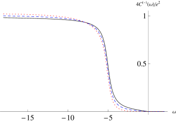
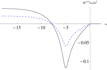
Figure 2: (Color online) Upper panel: the noise spectrum $C^{(-)}(\omega)$ for $V=0$ and $T=0$. Here $\epsilon_{d}=-5$ (energies and noise are measured in units of $\Gamma$). The three curves correspond to zero asymmetry $a=0$ (the black continuous curve), $a=0.7$ (the blue dashed curve), $a=1$ (the red dotted curve). Results are independent of the sign of $a$. Lower panel: the cross-correlation function $C^{(\times)}(\omega)$ for $a=0$ (black continuous curve) and $a=0.7$ (blue dashed curve).

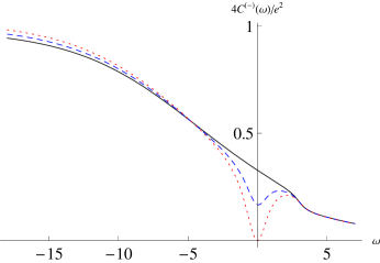
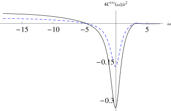
Figure 3: (Color online) Same as Fig. 2, but for $k_{B}T=4$.

III.2 The biased dot at $T=0$

When the dot is biased, the contributions of the four processes to the noise are all different. At $T=0$, and using Eq. (2), Eq. (II.2) becomes

$$\frac{8\pi}{e^{2}}C^{(\pm)}(\omega)=\Theta(-\omega)\int_{\frac{eV}{2}}^{\frac{eV}{2}-\omega}dEF^{(\pm)}_{LL}(E,\omega)$$

$$+\Theta(-\omega)\int_{-\frac{eV}{2}}^{-\frac{eV}{2}-\omega}dEF^{(\pm)}_{RR}(E,\omega)$$

$$+\Theta(eV-\omega)\int_{-\frac{eV}{2}}^{\frac{eV}{2}-\omega}dEF^{(\pm)}_{LR}(E,\omega)$$

$$+\Theta(-eV-\omega)\int_{\frac{eV}{2}}^{-\frac{eV}{2}-\omega}dEF^{(\pm)}_{RL}(E,\omega)\ .$$ (38)

Again, we start with $C^{(+)}(\omega)$. From Eq. (32) it follows that each integral in Eq. (38) will generate a step in $C^{(+)}(\omega)$ if a resonance at $E\sim\epsilon_{d}$ or at $E\sim\epsilon_{d}-\omega$ occurs within the range of integration, and this step will be weighed by the appropriate product $\Gamma_{\gamma}\Gamma_{\gamma^{\prime}}$. The upper part of Fig. 4 presents results for $C^{(+)}(\omega)$, for three values of the bias $V$. Comparing these figures with the curves in Fig. 1 one notes the following features. (i) As stated above, $C^{(+)}(\omega)$ always vanishes at $\omega=0$. At small $|\omega|$, the leading contribution comes from the third term in Eq. (38):

$$\frac{4}{e^{2}}C^{(+)}(\omega)\approx\frac{8\Gamma_{L}\Gamma_{R}}{\pi\Gamma^{4}}\omega^{2}\int_{-eV/2}^{eV/2}dE\sin^{4}\delta(E)\ .$$ (39)

Using also $\int dE\sin^{4}\delta(E)=(\Gamma/2)\int d\delta\sin^{2}\delta=\delta/2-\frac{1}{4}\sin(2\delta)$, and assuming that $|\epsilon_{d}|\ll|eV/2|$ so that the resonance is fully within the range of integration, we end up again with a parabolic dip, $4C^{(+)}(\omega)/e^{2}\approx(2\Gamma_{L}\Gamma_{R}/\Gamma^{3})\omega^{2}$. (ii) Unlike in Fig. 1, we now have a finite noise also for $\omega\geq 0$. This noise arises only from the ‘$LR$’ process, i.e. the third integral in Eq. (38) (note that $\mu_{L}>\mu_{R}$). From Eq. (32), the magnitude of this noise is of order $\Gamma_{L}\Gamma_{R}/\Gamma^{2}=(1-a^{2})/4$. It therefore vanishes for the maximal anisotropy, $|a|=1$, and does not depend on the sign of $a$ (and therefore the two curves with $a=\pm 0.7$ coincide for $\omega>0$). In the two upper left panels, we have $|\epsilon_{d}|\geq|eV/2|$, and we observe a plateau in $C^{(+)}(\omega)$ for $0<\omega<eV$, which decreases back to zero at both ends of this range. In contrast, the upper right panel in Fig. 4 corresponds to $|eV/2|>|\epsilon_{d}|$. In that panel we see that for $|a|<1$ the above single plateau splits into two plateaus, which arise at $\omega=eV/2\pm|\epsilon_{d}|$. These steps are due to two resonances which occur in the ‘$LR$’ process for these frequencies. (iii) For $\omega<0$, we no longer have symmetry under $a\rightarrow-a$. For $|a|=1$, we still have a single step in the noise, but this step now occurs at different frequencies for $a=1$ and $a=-1$. For $a=1$, this step arises due to the ‘$RR$’ process [second integral in Eq. (38)], and it emerges at $\omega=-|\epsilon_{d}+eV/2|$. For $a=-1$, this step arises due to the ‘$LL$’ process [first integral in Eq. (38)], and it occurs at $\omega=\epsilon_{d}-eV/2$. For $|a|<1$, the single step that appears in Fig. 1 at $\omega\simeq\epsilon_{d}$ splits under the effect of the bias into two steps, located at the same frequencies as for $a=\pm 1$. The plateau which appears between these two steps decreases as $a$ decreases from 1 to $-1$. One may trace this behavior to the different limits of the integrals, resulting from the different ranges allowed by the Fermi functions. For example, the ‘$LL$’ process [the first term in Eq. (38)] contributes once $\omega$ becomes smaller than $\epsilon_{d}-(eV/2)$ while the ‘$RR$’ one requires that $\omega<-|\epsilon_{d}+(eV/2)|$.

We next turn to the current correlations, $C^{(-)}(\omega)$, shown in the lower part of Fig. 4. As stated, the difference $C^{(\times)}(\omega)$ is small for large $|\omega|$. Indeed, in this range the two rows in Fig. 4 are very similar. The major differences arise for the shot noise, i.e. for small $|\omega|$. As explained after Eq. (39), the noise for $\omega\geq 0$ is fully due to the ‘$LR$’ process, i.e. the third term in Eq. (38). This term vanishes at $|a|=1$, and increases to its maximum as $|a|$ decreases to 0. When the bias is large enough, $|eV|-|\epsilon_{d}|>\Gamma$, for $\omega$ near 0, $C^{(-)}(\omega)$ is determined by the ‘$LR$’ process, given by Eq. (33). While the second term is the second line of Eq. (33) is relatively constant around $\omega=0$, the first term there is significant only when the two resonances overlap, i.e. within about $2\Gamma$ of $\omega=0$. Since this term is proportional to $a^{2}$, it introduces a positive peak in $C^{(-)}(\omega)$ as $|a|$ increases. This peak is indeed clearly seen in the lower right panel of Fig. 4.

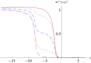
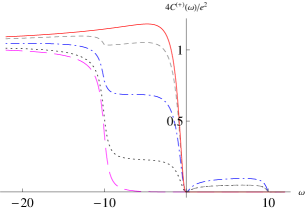
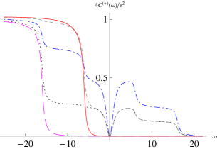
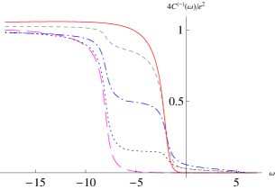
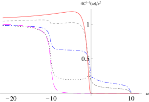
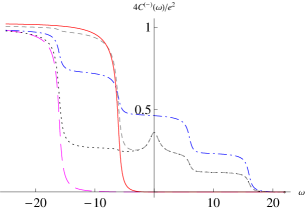
Figure 4: (Color online) The noise spectra $C^{(+)}(\omega)$ (upper panels) and $C^{(-)}(\omega)$ (lower panels) of the biased dot at zero temperature and $\epsilon_{d}=-5$, for $eV=6,~{}10$ and $22$ (left, center and right panels). All energies are measured in units of $\Gamma$. The five curves correspond to zero asymmetry ($a=0$, the dotted-dashed curve), $a=-0.7$ (the dotted curve) , $a=0.7$ (the small dashed curve), $a=-1$ (the long dashed curve), and $a=1$ (the continuous curve).

Unlike $C^{(+)}(\omega)$, which has continuous first and second derivatives at $\omega=0$, the slope of $C^{(-)}(\omega)$ is discontinuous at $\omega=0$ for $T=0$: in this limit the Fermi distribution can be replaced by a $\Theta$ function [as done in Eq. (38)], which has a discontinuous derivative (these discontinuities also generate discontinuities in the derivatives at other frequencies, but here we concentrate on the dip or peak in the shot noise). When $eV=\epsilon_{d}$, the second integral in Eq. (38), which corresponds to the ‘$RR$’ process, also exhibits a step at $\omega=0$. This integral, together with its $\Theta$ function, generate the discontinuity in the derivative of $C^{(-)}(\omega)$. Explicitly, we find

$$\frac{8\pi}{e^{2}}\Bigl{[}\frac{dC^{(-)}}{d\omega}\Big{|}_{\omega\rightarrow 0^{+}}-\frac{dC^{(-)}}{d\omega}\Big{|}_{\omega\rightarrow 0^{-}}\Bigr{]}$$

$$=(36\Gamma_{L}^{2}\Gamma_{R}^{2}/\Gamma^{4})\bigl{(}\sin^{4}\delta(eV/2)+\sin^{4}\delta(-eV/2)\bigr{)}.$$ (40)

Thus, the discontinuities are largest when $|a|=1$ and when $|\epsilon_{d}|=|eV/2|$, as can be seen in the lower central panel in Fig. 4. This panel also shows a shift of the peak for $a=-0.7$, to a negative frequency.

III.3 Finite temperature

As we showed for $V=0$, finite temperature broadens and smears the limits of the integrals of Eq. (II.2). Indeed, Fig. 5 exhibits such a smearing for $eV=22$ and $k_{B}T=3$. We show only this value of the bias, since the plots are qualitatively similar for smaller biases. The main new qualitative effect (compared to $T=0$) is the splitting of the curves for $\pm|a|$ ($a=\pm 0.7$ in Fig. 5) at $\omega>0$, due to the contributions of the ‘$LL$’ and ‘$RR$’ processes there [see Eq. (32)]. For $a>0$, the chemical potential $\mu_{R}$ is closer to $\epsilon_{d}$ (compared to $\mu_{L}$). Therefore, the right lead is more strongly connected to the dot, and this increases the contribution from the ‘RR’ process, which now integrates over two resonances. This is responsible for the dip in $C^{(-)}(\omega)$. At high temperatures, when the ‘$LL$’ process also integrates over two resonances, the peak in $a=-0.7$ would also turn into a dip.

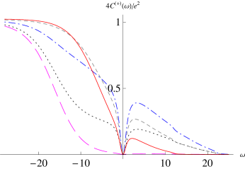
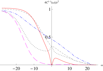
Figure 5: (Color online) The two noise spectra of the biased dot at $k_{B}T=3$, for $eV=22$ and $\epsilon_{d}=-5$ (all energies and noise are measured in units of $\Gamma$). The five curves correspond to zero asymmetry (the dotted-dashed curve), $a=-0.7$ (the dotted curve) , $a=0.7$ (the small dashed curve), $a=-1$ (the big dashed curve), and $a=1$ (the continues curve).

IV Summary

At $T=0$ and $V=0$, the noise spectrum of an unbiased single level quantum dot exhibits a single step around $\omega\simeq\epsilon_{d}$, whose shape depends very weakly on the spatial asymmetry of the dot or on the fluctuating quantity (current or charge). In this paper we found how the current and the charge fluctuations spectra develop additional functional features when studied at a finite bias and/or a finite temperature. These features also depend on the dot asymmetry parameter $a$. Since this parameter can be varied experimentally, using appropriate gate voltages, our results suggest several new measurements, which could yield information on the physics of the quantum dot.

At low temperatures and zero bias, the charge correlation function $C^{(+)}(\omega)$ should not depend on the asymmetry. However, even at zero bias, raising the temperature yields a dip around zero frequency. In contrast, the current correlation function $C^{(-)}(\omega)$ does depend on the asymmetry, and even at zero bias and finite $T$ it has a dip around $\omega=0$ whose depth decreases with decreasing asymmetry. The details of these dips may best be observed by measuring the cross-correlations between the currents on the two leads, $C^{(\times)}(\omega)$.

At finite bias and $T=0$, the single step mentioned above can split into two or four steps, depending on asymmetry and bias. Again, the experimental confirmation of the features shown in Fig. 4 can also give information on the location of the resonance and on its partial widths. It would be particularly interesting to study the various noise functions in the shot-noise region, where we find a variety of dips and peaks. At finite temperatures we also predict that for a finite asymmetry some dips can turn into peaks.

Acknowledgement

We thank Y. Imry, S. Gurvitz, A. Schiller, D. Goberman, V. Kashcheyevs, and V. Puller for valuable discussions. This work was supported by the German Federal Ministry of Education and Research (BMBF) within the framework of the German-Israeli project cooperation (DIP), and by the Israel Science Foundation (ISF).

References

- (1) R. Landauer, Nature 392, 658 (1998).
- (2) Y. Imry, Introduction to Mesoscopic Physics, 2nd ed. (Oxford University Press, Oxford, 2002).
- (3) Ya. M. Blanter and M. Büttiker, Phys. Rep. 336, 1 (2000).
- (4) L. Y. Chen and C. S. Ting, Phys. Rev. B 43, 4534 (1991).
- (5) D. V. Averin, J. Appl. Phys. 73, 2593 (1993).
- (6) H. A. Engel and D. Loss, Phys. Rev. Lett. 93, 136602 (2004).
- (7) O. Entin-Wohlman, Y. Imry, S. A. Gurvitz, and A. Aharony, Phys. Rev. B 75, 193308 (2007).
- (8) M. Büttiker, Phys. Rev. B 46, 12485 (1992).
- (9) M. Büttiker, A. Prêtre, and H. Thomas, Phys. Rev. Lett. 70, 4114 (1993).
- (10) M. Büttiker, Phys. Rev. B 45, 3807 (1992).
- (11) Y. Levinson, Phys. Rev. B 61, 4748 (2000).
- (12) U. Gavish, Y. Levinson, and Y. Imry, Phys. Rev. Lett. 87, 216807 (2001); U. Gavish, Y. Levinson, and Y. Imry, Phys. Rev. B 62, R10637 (2000).
- (13) A. Schiller, private communication.
- (14) T. K. Ng and P. A. Lee, Phys. Rev. Lett. 61, 1768 (1988).