Mean Field Model of Coagulation and Annihilation Reactions In a Medium of Quenched Traps: Subdiffusion

Abstract

We present a mean field model for coagulation ($A+A\rightarrow A$) and annihilation ($A+A\rightarrow 0$) reactions on lattices of traps with a distribution of depths reflected in a distribution of mean escape times. The escape time from each trap is exponentially distributed about the mean for that trap, and the distribution of mean escape times is a power law. Even in the absence of reactions, the distribution of particles over sites changes with time as particles are caught in ever deeper traps, that is, the distribution exhibits aging. Our main goal is to explore whether the reactions lead to further (time dependent) changes in this distribution.

I Introduction

Chemical reactions limited by the motions of the reactants are abundant in nature, and among the most thoroughly studied are diffusion-limited reactions. A ubiquitous approach to these systems simply adds the diffusion and reaction contributions together so as to construct appropriate reaction-diffusion equations. It is implicit and even explicit in these approaches that the diffusive component describes a motion without a memory, and if one invokes an underlying continuous time random walk (CTRW) where walkers react when they meet, it is understood that the waiting time distributions for reactants to remain at one location before moving on have a finite mean. The most frequently invoked waiting time in this scenario is exponential. It is also understood that in fact many microscopic models can be subsumed under the same mesoscopic reaction-diffusion umbrella havlin87 ; benavraham00 ; blumen86 ; kang85 ; toussaint83 .

On the other hand, contrary to the diffusive case, it is by now fairly clear that different microscopic scenarios of reactions among subdiffusive species, even simple scenarios, lead to different mesoscopic descriptions sokolov06 ; henry06 ; seki03 ; sagues08 ; reichman08 . For instance, a popular mesoscopic vehicle, the CTRW, involves waiting time distributions of ensembles of particles undergoing reactions. The forms of these distributions depend on the underlying microscopic rules and may vary from one microscopic scenario to another. It is thus risky to simply assume a form for these distributions as one would for diffusive particles. Instead, a more detailed derivation starting from a set of microscopic rules to arrive at a mesoscopic CTRW description is necessary. The specific microscopic reaction scenario of interest to us is a lattice whose sites are occupied by traps of varying depths, that is, the quenched trap scenario. If independent particles simply walk on this lattice, their escape time from each trap is exponentially distributed, with the distribution of trap depths reflected in a distribution of mean escape times. An average over this distribution leads to a CTRW model in which all sites have the same waiting time distribution scher ; klafter.silbey . This latter process is spatially homogeneous and semi-Markovian, and anomalous diffusion arises if the resulting mean waiting time on each site diverges. This is the so-called annealed trap scenario. However, if particles can also react with one another, interesting questions immediately arise. Of interest to us are the reactions $\mathrm{A}+\mathrm{A}\rightarrow\mathrm{A}$ (coagulation) and $\mathrm{A}+\mathrm{A}\rightarrow 0$ (annihilation); some uncertainties arising from different microscopic descriptions can be illustrated with the coagulation reaction. Suppose there is an $\mathrm{A}$ at a site, and a second $\mathrm{A}$ arrives. In the underlying spatially disordered quenched trap model, it does not matter which particle is “killed” by the reaction since the waiting time distribution for particle departure from any site is exponential. Such a process is often called memoryless because the future of each particle is determined only by its present state and not its past, and therefore the differences between the two victims become irrelevant. However if, as we subsequently do, we implement a mean field assumption which turns out to lead to a description that is asymptotically equivalent to a CTRW with diverging mean waiting times, that is, to an annealed trap model, it may make a kinetic difference which of the two particles is “killed” in each reaction. It is not clear in general how to include such fine distinctions in a mesoscopic formalism, nor is it clear what sort of rule at the mesoscopic or mean field level best mimics the behavior of the underlying trapping problem.

Our mean field model shares with other CTRW models with diverging mean waiting times the phenomenon of “aging” bouchaud2 ; monthus ; barkai ; jsp . Even in non-reactive systems, aging causes the waiting time distribution itself to change with time as particles settle into sites with ever longer waiting times (corresponding to particles caught in ever deeper traps in the underlying system). Aging for non-reactive particles does not occur in a given finite quenched trap environment since the distribution of particles approaches a Boltzmann distribution barkai2 . The most intriguing unanswered question that we address in this work is whether the reactions cause a change in the waiting time distribution. We anticipate our answer to this latter question: we find that in our mean field model the reaction does not cause an additional change in the waiting time distribution.

We will compare our model predictions with the results of numerical simulations of the actual distributed trap scenario. We find that the mean field approach works well for higher dimensions ($d\geq 3$) but not for low dimensions ($d=1$), a result that agrees with the well-known differences in subdiffusion exponents predicted by CTRW theories and those obtained by numerical simulations in the absence of reactions bouchaud The concentrations of surviving particles are known to be well reproduced in all dimensions by invoking relations with the number of distinct sites visited in the asymptotically equivalent CTRW blumen86 ; ourchapter . On the other hand, the mean field formalism, while restricted to higher dimensions, provides additional direct insights into the more detailed information contained in the time dependence of the waiting time distributions.

In Sec. II we describe our mean field model and arrive at a master equation for the density of particles with given mean rate for leaving any site in the absence of reactions. This equation explicitly shows the effects of aging. In Sec. III we establish the corresponding master equations in the presence of the coagulation and annihilation reactions. In Sec. IV we discuss the solution of the master equation for the time-dependent rate distribution. Comparisons with numerical simulation results for the underlying random trap model are presented in Sec. V. We conclude with a brief summary in Sec. VI.

II Mean-field approach to a trap model

To construct a mean field model, we start with a lattice whose sites are traps of varying depths. Our model is equivalent to that of monthus , but our notation is suitably modified to facilitate the inclusion of reactions, which they do not consider. The waiting time for leaving a trap $i$ is exponentially distributed, $p(t|\tau)=\tau_{i}^{-1}\exp(-t/\tau_{i})$, where $\tau_{i}$, the mean sojourn time in the trap, is determined by the trap’s depth via the Kramers (Arrhenius) law. We further assume that the distribution of mean waiting times is a power law, for example, $p(\tau)=\gamma\tau^{-1-\gamma}\theta(\tau-1)$. Note that the asymptotics of the pdf $\psi(t)$ of waiting times $t$ upon averaging over this distribution of mean waiting times is then of power law form even though the waiting time for each trap is exponentially distributed, i.e.,

$$\psi(t)=\int_{0}^{\infty}p(t|\tau)p(\tau)d\tau\sim\gamma\Gamma(1+\gamma)\tau^{-1-\gamma}.$$ (1)

The power law distribution of mean waiting times $\tau_{i}$ leads to a power law distribution of the “leaving rates” $\omega_{i}=1/\tau_{i}$ for departing from a site,

$$p(\omega)=\gamma\omega^{\gamma-1}\theta(1-\omega).$$ (2)

Note that all the moments of the distribution of the rates are finite even if those of the waiting time distribution are not.

Particles are distributed over sites with different mean waiting times, and as time proceeds, the distribution of particles over these sites changes even in the absence of reactions because more and more particles get stuck in deeper and deeper traps. Our central question concerns the effects of reactions on this evolving distribution. In particular, we ask whether the distribution is modified by the reactions. This is difficult to answer, at least analytically, without further approximation. The system with distributed traps of varying depths is spatially inhomogeneous, and if the particle executes the usual nearest neighbor random walk, the future of any particle moving over this landscape may be strongly dependent on its particular location. Furthermore, there may be strong correlations among subsequent steps (especially in lower dimensions) because the particle may revisit a previously visited site. To make progress we implement a mean field approximation designed to provide information about the evolving distribution of particles over the inhomogeneous landscape. Specifically, we assume that the particles do not perform a nearest neighbor random walk but instead that each particle is equally likely (probability $1/N$) to step on any of the $N$ sites of the system. In other words, the lattice is a complete graph. Equivalently, as an alternative way of viewing the model, we can think of particles performing nearest neighbor random walks, but before each step the mean waiting time associated with the trap to which the particle is about to step is chosen anew from the distribution $p(\tau)$ or, correspondingly, a new leaving rate is chosen from $p(\omega)$, independently of the waiting times chosen in prior steps. It is also equivalent to a nearest neighbor CTRW in a very high-dimensional quenched medium. In any case, in the absence of reactions this results in a space-homogeneous CTRW model with waiting time distribution $\psi(t)$ as given in Eq. (1) chosen anew at each step.

The assumptions underlying the mean field approach are expected to be more adequate for random walks that are transient, that is, ones in which already visited sites are revisited only with a small probability so that almost all sites reached by the walker are new sites. This is the case for random walks in dimensions $d\geq 3$ and, as we show in Sec. V, we do find excellent agreement between the mean field approach and numerical simulations for the reactions in quenched trap environments for $d\geq 3$. If the walk is recurrent, that is, if the same sites are revisited repeatedly, the approximation may be poor. One-dimensional walks are recurrent, and $d=2$ is the marginal dimension for this property.

As noted earlier, as time evolves the distribution of particles over the sites with given mean waiting times (leaving rates) changes even in the absence of the reactions because more and more particles get stuck in deeper and deeper traps. We discuss these changes first in the absence and then in the presence of the reactions. For this purpose we note that under the mean field assumption, the master equation for the probability $a_{i}(t)$ to be at site $i$ at time $t$ reads

$$\frac{d}{dt}a_{i}(t)=\frac{1}{N}\sum_{j\neq i}\omega_{j}a_{j}(t)-\omega_{i}a_{i}(t).$$ (3)

Since each site is characterized by its own $\omega$, we can pass from the occupation probability $a_{i}$ to the probability $a(\omega,t)$ and introduce the density $n(\omega,t)$ of particles occupying sites with leaving rate between $\omega$ and $\omega+d\omega$. One easily deduces that $n(\omega,t)d\omega=a(\omega,t)p(\omega)d\omega$, where $Np(\omega)d\omega$ is the number of sites with leaving rates between $\omega$ and $\omega+d\omega$. Note that in a large system

$$\frac{1}{N}\sum_{j\neq i}\omega_{j}a_{j}(t)\simeq\frac{1}{N}\int\omega Np(\omega)a(\omega,t)d\omega=\int\omega n(\omega,t)d\omega.$$ (4)

The last integral can be associated with the time-dependent mean rate,

$${\Omega}(t)=\int\omega n(\omega,t)d\omega.$$ (5)

Multiplying both sides of Eq. (3) by $p(\omega)$ leads to the master equation for $n(\omega,t)$,

$$\frac{d}{dt}n(\omega,t)={\Omega}(t)p(\omega)-\omega n(\omega,t).$$ (6)

This equation governs the change in the distribution of particles over jump rates in the absence of reactions. Note that the total concentration of particles $c=\int n(\omega,t)d\omega$ is constant in time.

III Rate distribution with reactions

Next we explore the effects of reactions on the site occupation probabilities. We assume that the usual law of mass action is appropriate at the local level. For the case of the $\mathrm{A}+\mathrm{A}\rightarrow\mathrm{A}$ reaction within our mean-field approximation, the change in the occupation probability at site $i$ is

$$\frac{d}{dt}a_{i}(t)=[1-a_{i}(t)]\frac{1}{N}\sum_{j\neq i}\omega_{j}a_{j}(t)-\omega_{i}a_{i}(t)$$ (7)

since the number of particles at a site already occupied by a particle [with probability $a_{i}(t)$] does not change upon the arrival of the new particle. In the case of the $\mathrm{A}+\mathrm{A}\rightarrow 0$ reaction the number of particles at an occupied site is reduced by one upon the arrival of a new particle, so that the corresponding equation reads

$$\frac{d}{dt}a_{i}(t)=[1-2a_{i}(t)]\frac{1}{N}\sum_{j\neq i}\omega_{j}a_{j}(t)-\omega_{i}a_{i}(t).$$ (8)

Again we can focus instead on $n(\omega,t)$, but this is no longer a proper probability density because the total number of particles is not conserved. Regrouping terms one obtains the reaction equations

$$\frac{d}{dt}n(\omega,t)=p(\omega)\int_{0}^{\infty}\omega n(\omega,t)d\omega-\left[\omega+\int_{0}^{\infty}\omega n(\omega,t)d\omega\right]n(\omega,t)$$ (9)

for the $\mathrm{A}+\mathrm{A}\rightarrow\mathrm{A}$ reaction, and

$$\frac{d}{dt}n(\omega,t)=p(\omega)\int_{0}^{\infty}\omega n(\omega,t)d\omega-\left[\omega+2\int_{0}^{\infty}\omega n(\omega,t)d\omega\right]n(\omega,t)$$ (10)

for $\mathrm{A}+\mathrm{A}\rightarrow 0$. At $t=0$ the particles are homogeneously distributed over all sites in the system, so the initial condition for $n$ is $n(\omega,0)=p(\omega)$. A normalized probability density is obtained by noting that the overall time-dependent reactant concentration is given by

$$c(t)=\int_{0}^{\infty}n(\omega,t)d\omega.$$ (11)

The properly normalized probability density of particles occupying sites with leaving rate between $\omega$ and $\omega+d\omega$ is then given by

$$p(\omega,t)=\frac{n(\omega,t)}{c(t)}.$$ (12)

We again introduce the time-dependent mean jumping rate, which is now given by

$${\Omega}(t)=c^{-1}(t)\int_{0}^{\infty}\omega n(\omega,t)d\omega=\int_{0}^{\infty}\omega p(\omega,t)d\omega,$$ (13)

and rewrite Eqs. (9) and (10) in the form

$$\frac{d}{dt}n(\omega,t)=c(t){\Omega}(t)p(\omega)-[\omega+c(t){\Omega}(t)]n(\omega,t)$$ (14)

for the $\mathrm{A}+\mathrm{A}\rightarrow\mathrm{A}$ reaction, and

$$\frac{d}{dt}n(\omega,t)=c(t){\Omega}(t)p(\omega)-[\omega+2c(t){\Omega}(t)]n(\omega,t)$$ (15)

for the $\mathrm{A}+\mathrm{A}\rightarrow 0$ reaction. Integrating these two equations over the $\omega$-domain gives the classical kinetic equations

$$\frac{d}{dt}c(t)=-\mu{\Omega}(t)c^{2}(t)$$ (16)

with the stoichiometric coefficient (“molarity”) of the reaction $\mu=1$ for the $\mathrm{A}+\mathrm{A}\rightarrow\mathrm{A}$ reaction and $\mu=2$ for $\mathrm{A}+\mathrm{A}\rightarrow 0$. The mean jump rate $\Omega(t)$ is thus the time-dependent reaction rate.

The equation for the probability density $p(\omega,t)=n(\omega,t)c^{-1}(t)$ corresponding to Eqs. (14) and (15) is then

$$\frac{d}{dt}p(\omega,t)+p(\omega,t)\frac{1}{c(t)}\frac{d}{dt}c(t)={\Omega}(t)p(\omega)-\omega p(\omega,t)-\mu c(t){\Omega}(t)p(\omega,t).$$ (17)

With Eq. (16) we see that the term with the time derivative $dc/dt$ on the left side of this equation and the last term on the right side cancel. Thus, the final equation for $p(\omega,t)$ does not depend on the molarity $\mu$ of the reaction and is the same as the equation for $n(\omega,t)$ in the absence of reactions,

$$\frac{d}{dt}p(\omega,t)={\Omega}(t)p(\omega)-\omega p(\omega,t).$$ (18)

This statement also leads to the remarkable conclusion that within the mean field approximation adopted in this model the reaction does not affect the waiting time distribution. This answers one of our main questions.

IV Solution for the time-dependent rate distribution

The principal question posed earlier, namely, whether the reaction changes the waiting time distribution, has been answered in the negative within our mean-field approach. It is now instructive to obtain an explicit expression for the time dependent reaction rate. Equation (18) is an integro-differential equation for $p(\omega,t)$ since ${\Omega}(t)$ as defined in Eq. (13) depends on $p(\omega,t)$ itself. However, contrary to the equations for $n(\omega,t)$, this equation is linear and can best be approached via Laplace transforms. First we consider the time-Laplace transforms of $p(\omega,t)$ and ${\Omega}(t)$,

$$\tilde{p}(\omega,s)=\int_{0}^{\infty}p(\omega,t)e^{-st}dt,\qquad\tilde{\Omega}(s)=\int_{0}^{\infty}{\Omega}(t)e^{-st}dt.$$ (19)

The transform of Eq. (18) is

$$s\tilde{p}(\omega,s)-p(\omega)=\tilde{\Omega}(s)p(\omega)-\omega\tilde{p}(\omega,s),$$ (20)

where we have explicitly used the initial condition $p(\omega,0)=p(\omega)$. The formal “solution” for $\tilde{p}(\omega,s)$ (with $\tilde{p}$ still contained in $\tilde{\Omega}$) is

$$\tilde{p}(\omega,s)=[1+\tilde{\Omega}(s)]\frac{p(\omega)}{s+\omega}.$$ (21)

Transforming the definition (13) of ${\Omega}(t)$ we obtain

$$\tilde{\Omega}(s)=\int_{0}^{\infty}\tilde{p}(\omega,s)\omega d\omega,$$ (22)

so that multiplying both sides of Eq. (21) by $\omega$ and integrating, we arrive at a closed algebraic equation for $\tilde{\Omega}(s)$,

$$\tilde{\Omega}(s)=[1+\tilde{\Omega}(s)]\int_{0}^{\infty}\frac{\omega p(\omega)}{s+\omega}d\omega.$$ (23)

The solution of this equation is

$$\tilde{\Omega}(s)=\frac{\tilde{I}(s)}{1-\tilde{I}(s)},$$ (24)

where

$$\tilde{I}(s)\equiv\int_{0}^{\infty}\frac{\omega p(\omega)}{s+\omega}d\omega.$$ (25)

The integral representing $I(s)$ can be evaluated asymptotically for any long-tailed distribution $p(\tau)$ using the asymptotic method for integrals with weak singularity (see Ch. 1 §4 in Fedoryuk ), as follows. We can rewrite $I(s)$ as

$$I(s)=1-s\int_{0}^{\infty}\frac{p(\omega)}{s+\omega}d\omega=1-s\int_{0}^{\varepsilon}\frac{p(\omega)}{s+\omega}d\omega-s\int_{\varepsilon}^{\infty}\frac{p(\omega)}{s+\omega}d\omega$$ (26)

for any $\varepsilon$. Relevant to the long-time asymptotic behavior is the small-$s$ behavior of $I(s)$. As long as $\varepsilon$ is chosen such that $\varepsilon/s\to\infty$ as $s\to 0$, the third integral on the right hand side is of $O(1)$ in this limit. Furthermore, if $p(\omega)\sim\gamma\omega^{\gamma-1}$ as $\omega\to 0$ and $\varepsilon\ll 1$, we can write

$$I(s)\underset{s\to 0}{\sim}1-s\gamma\int_{0}^{\varepsilon}\frac{\omega^{\gamma-1}}{s+\omega}d\omega-O(s)\text{\quad with\quad}\varepsilon\ll 1.$$ (27)

Finally, a change of variables $z=\varepsilon/s$ then allows us to write for $s\to 0$

$$I(s) \sim 1-\gamma s^{\gamma}\int_{0}^{z\to\infty}\frac{z^{\gamma-1}}{1+z}dz-O(s)$$ (28)

$$\sim 1-\frac{\gamma\pi}{\sin\pi\gamma}s^{\gamma}.$$

For the particular form $p(\omega)=\gamma\omega^{\gamma-1}\Theta(1-\omega)$ introduced earlier, one finds the result valid for all $s$ [Abramowitz and Stegun formula 15.3.1]

$$\tilde{I}(s)=\frac{\gamma}{(1+\gamma)s}~{}_{2}F_{1}(1,1+\gamma,2+\gamma,-1/s),$$ (29)

which for small $s$ (relevant to long-time asymptotic behavior) leads to the second line of Eq. (28). The inverse transform of $\tilde{\Omega}(s)$ then follows upon application of the Tauberian theorem,

$${\Omega}(t)\sim\frac{\sin\pi\gamma}{\gamma\pi\Gamma(\gamma)}t^{\gamma-1}.$$ (30)

We have thus provided a mesoscopic theoretical foundation for the widely accepted result that the reaction rate decays with time.

The time dependent reaction rate can now be inserted in the rate equation (16) to solve for the concentration as a function of time. At long times we find the explicit result

$$c(t)\sim\frac{\pi\gamma\Gamma(1+\gamma)}{\mu\sin\pi\gamma}t^{-\gamma}.$$ (31)

We can in fact calculate the full rate distribution by integrating Eq. (18). The result up to quadrature is

$$p(\omega,t)=p(\omega)e^{-\omega t}\left[\int_{0}^{t}dt^{\prime}e^{\omega t^{\prime}}\Omega(t^{\prime})+1\right].$$ (32)

From this, we can extract the $\omega$ dependence for short times $\omega t\ll 1$ as $p(\omega,t)\sim p(\omega)$ and for long times $\omega t\gg 1$ as $p(\omega,t)\sim p(\omega)/\omega$.

Finally, we note the interesting connections between these results and the number $S(t)$ of distinct sites visited up to time $t$ by a particle in a CTRW YKKbriefreport . We can connect this quantity to the average reaction rate $\Omega(t)$ for $d\geq 3$ as follows. Since at each step of the process a particle mostly visits a new site in the system (the random walk is “transient” or “non-recurrent”), the reaction rate can be approximated by the time derivative of the number of newly visited sites, $\Omega(t)=dS/dt$, and we have YKKbriefreport

$$\tilde{S}(s)\sim\frac{1}{s}\frac{1-R}{1-\tilde{\psi}(s)},\quad s\to 0$$ (33)

where $R$ is the probability of return to the origin ($R=0.3405\ldots$ for a simple cubic lattice). Note that the small-$s$ behavior of $\tilde{\psi}(s)$ corresponding to the asymptotic behavior of $\psi(t)$ in Eq. (1) is

$$\tilde{\psi}(s)\sim 1-\frac{\gamma\pi}{\sin\pi\gamma}s^{\gamma}\equiv 1-(s/\lambda)^{\gamma}$$ (34)

Inserting this expression into (33), inserting (28) into (24), and comparing the resulting expressions, one sees that $S(s)\sim(1-R)\tilde{\Omega}(s)/s$ for small $s$, so that $\Omega(t)\sim(1-R)dS/dt$ for large $t$. Although the interpretation of the reaction rate in terms of the number of distinct sites visited is quite standard, the fact that the broad distribution of trapping times does not introduce any additional fluctuation effects into the kinetics is not at all trivial.

A further connection with the distinct number of sites visited in a CTRW occurs for the concentration of surviving reactant, namely, $c(t)\sim 1/S(t)$, a connection that holds not only for $d>2$ but also for $d\leq 2$, i.e., even when the random walk is recurrent blumen86 ; ourchapter . In YKKbriefreport we explicitly obtained the $3d$ result $S(t)\sim[(1-R)/\Gamma(1+\gamma)](\lambda t)^{\gamma}$. In one dimension $S(t)\sim[\sqrt{2}/\Gamma(1+\gamma/2)](\lambda t)^{\gamma/2}$. We will test the proposition that $c(t)\sim 1/S(t)$ in the next section along with results of the theory we have developed above.

V Numerical results

Our discussion supports the expectation that the results of the mean field model approximate those of the underlying random depth trap system in $3d$ (but not in $1d$). Even in $3d$, where walks are transient, it is nevertheless the case that there is a finite probability $R$ of return to a previously visited site, e.g. about 1/3 for a simple cubic lattice. In this section we compare our results with those of numerical simulations of $3d$ and $1d$ lattices with traps of random mean exit times as described earlier. The algorithm used in the simulations is described in some detail in the Appendix.

Figure 1 shows a collection of results for the concentration of reactants as a function of time in $3d$. The results fall essentially on two straight lines, except for finite size effects. The upper set of results is for $\gamma=0.5$ and the lower set for $\gamma=0.8$. The concentrations shown are indicated as $c_{1}(t)$, which we associate with the coagulation reaction $\mathrm{A}+\mathrm{A}\rightarrow\mathrm{A}$, and $c_{2}(t)$ for the annihilation reaction $\mathrm{A}+\mathrm{A}\rightarrow 0$. We plot $c_{1}(t)$ and $2c_{2}(t)$ to ascertain that the surviving concentration in the coagulation reaction is twice that of the annihilation reaction. The coincidence of the simulation results for the two cases shows that this is indeed the case. Simulation results are shown for two sizes of the $L\times L\times L$ simple cubic lattice with $L=30$ and $L=60$. The results for the two sizes are the same except for the larger value of $\gamma$, where we see some deviations from the straight line at very long times due to finite size effects. These deviations are more pronounced for the larger $\gamma$ (in the faster walk the ends of the lattices are reached earlier) and for the smaller lattice. Since this is a log-log plot the straight-line behavior confirms the power law decay of the concentrations. Furthermore, we find that the slopes of these lines are close to $\gamma$. In particular, we find slopes $0.491(2)$ for $\gamma=0.5$ and $0.763(2)$ for $\gamma=0.8$ (in both cases for both reactions). The agreement in the former case is very good, but somewhat less so in the latter, where we are not in the fully asymptotic scenario footnote .

Figure 2 shows our simulation results in $1d$, again for $\gamma=0.5$ and $\gamma=0.8$. The lines in this case are power law fits to the simulation results. The size of the lattice is $L=10,000$. The mean field approach is not valid here as an approximation to the underlying trap model, and yet a number of interesting results are nevertheless worth mentioning. First, we note that the relation $c_{1}(t)=2c_{2}(t)$ still holds. We do not know whether this indicates that here again the reactions do not affect the dynamics of the moving species, but this result indicates that it may be so. Second, we note that the exponents of the concentration, while quite different from those of the mean field model, agree with those associated with the distinct number of sites visited for the original trap model, namely, that in one dimension $c(t)\sim 1/S(t)\sim\left\langle x^{2}\right\rangle^{-1/2}\sim t^{-\gamma/(1+\gamma)}$ because all sites within the span of the random walk are visited at least once. The numerical fits for the simulation results yield $c_{1}(t)=2c_{2}(t)\sim 0.881(1)t^{-0.3328(1)}$ for $\gamma=0.5$ and $c_{1}(t)=2c_{2}(t)\sim 0.959(4)t^{-0.430(1)}$ for $\gamma=0.8$. The exponents $0.33$ and $0.43$ are in good agreement with the values of $\gamma/(1+\gamma)=0.333$ and $0.444$ respectively.

Finally, we compare our analytic mean field predictions in more detail with numerical simulations of the quenched trap model. In Fig. 3 we show results for the distribution $p(\omega,t)$ vs $\omega$. The solid lines in both panels correspond to the mean field result (32) for $\gamma=0.5$. From high to low on the right side of each panel the curves are for $t=10^{2}$, $10^{3}$, $10^{4}$, and $10^{5}$. Equation (32) leads to $p(\omega,t)\sim p(\omega)\sim\omega^{\gamma-1}$ for $\omega t\ll 1$ and $p(\omega,t)\sim p(\omega)/\omega\sim\omega^{\gamma-2}$ for $\omega t\gg 1$; the slopes $-0.5$ and $-1.5$ in the log-log plot are evident. The symbols show the corresponding simulation results. The top panel shows the results for a $3d$ quenched trap lattice with nearest neighbor steps, and the bottom panel those of of a quenched trap lattice in which steps to any site are equally likely. Our only adjustment in these figures is the normalization, which can not be obtained properly from the simulations since they do not cover an infinite range of $\omega$s. We have made this adjustment by scaling the simulation results so that the quantity $R(t)=\int_{\omega_{min}}^{\omega_{max}}P(\omega,t)d\omega<1$ evaluated using the scaled results agrees with the one obtained by means of the theoretical result (32). Here $\omega_{min}$ and $\omega_{max}$ define the range of $\omega$s covered by the simulations. These results confirm that already in $3d$ the mean field theory captures the behavior as well as does the actual numerical realization of the model. We have also ascertained the agreement between simulations and mean field theory for other values of the subdiffusive exponent $\gamma$.

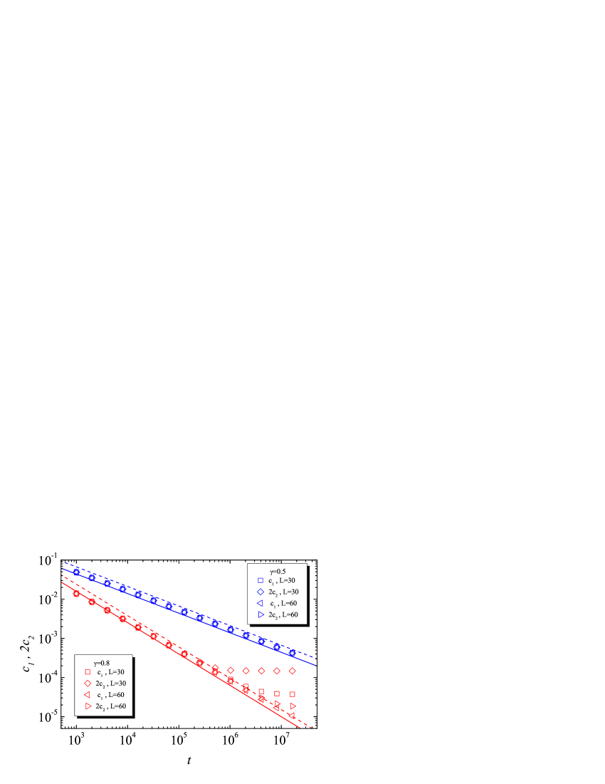
Figure 1: The reactant concentrations $c_{1}(t)$ and $2c_{2}(t)$ in three dimensions as functions of time for $\gamma=0.5$ and $\gamma=0.8$ and two lattice sizes. The symbols denote numerical simulation results. The solid lines result from the mean field theory, and the dashed lines from the connection with the number of distinct sites visited.

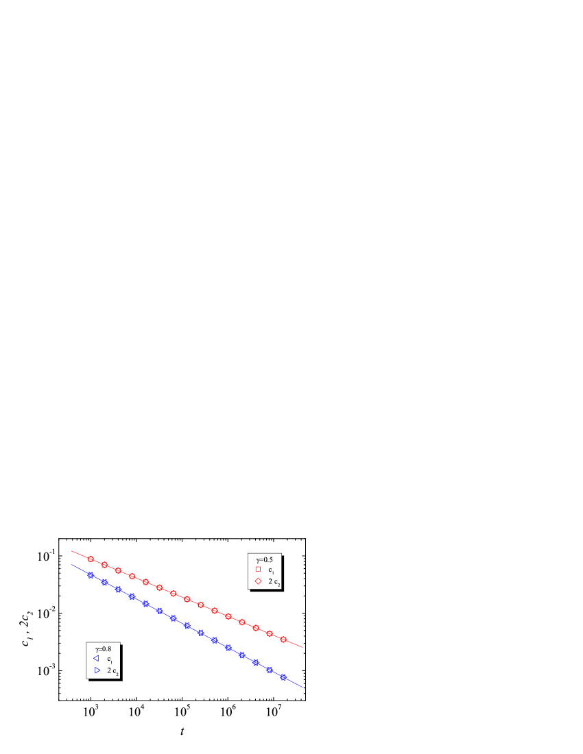
Figure 2: The reactant concentrations $c_{1}(t)$ and $2c_{2}(t)$ in one dimension as functions of time for $\gamma=0.5$ and $\gamma=0.8$. The symbols denote the results of numerical simulations, and the lines are linear fits to these results.

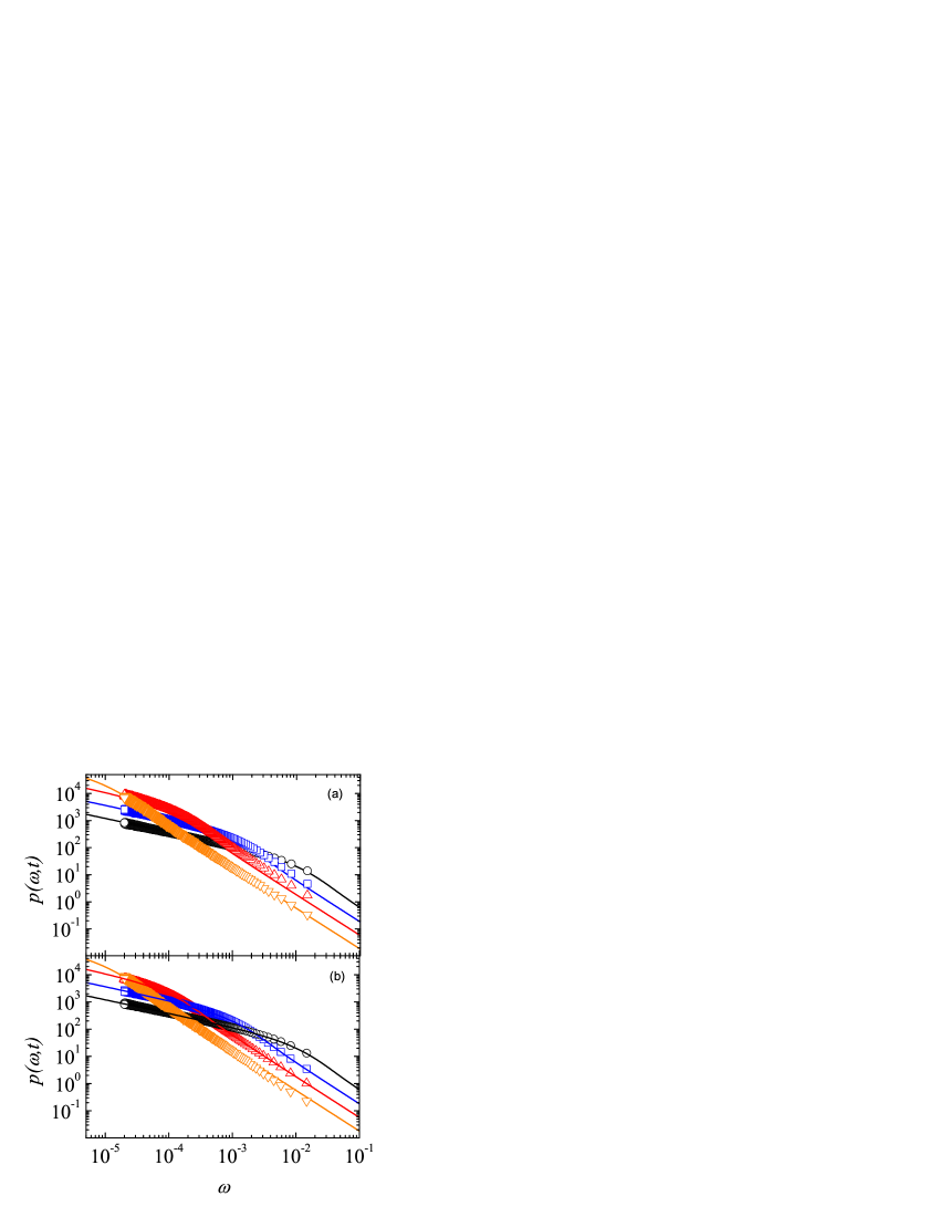
Figure 3: For all results in this figure, $\gamma=0.5$. The solid lines are calculated from the analytic result Eq. (32) and the symbols are the simulation results for lattices with quenched traps scaled as described in the text. From high to low on the right side of each panel the curves are for $t=10^{2}$, $10^{3}$, $10^{4}$, and $10^{5}$. Top panel: $3d$ lattice; bottom panel: lattice with equally likely jumps to any site, that is, a complete graph.

VI Conclusions

We have presented a mean field theory of for coagulation ($\mathrm{A}+\mathrm{A}\rightarrow\mathrm{A}$) and annihilation ($\mathrm{A}+\mathrm{A}\rightarrow 0$) reactions on a lattice whose sites are occupied by traps of varying depths. The escape times from these traps are distributed exponentially about a mean time, and the distribution of mean escape times is of power law form. We calculate reactant concentrations as a function of time as well as the time-dependent distribution of particles over sites with different escape rates. The mean field model is designed with the particular goal of studying this evolving distribution and the effects of the reactions on it, and is expected to do well in dimensions $d\geq 3$ but not in $1d$. The noteworthy outcome of the model is that this distribution is not changed by the occurrence of the reactions. One consequence of this result is that the concentration of surviving reactant in the $A+A\rightarrow A$ reaction is double that of the $A+A\rightarrow 0$ reactions, that is, $c_{1}(t)=2c_{2}(t)$. While the model does not shed light on the $1d$ case, numerical simulations here also show that $c_{1}(t)=2c_{2}(t)$ and thus a reaction-insensitive aging distribution of particles is not ruled out. Numerical simulations in $d=3$ with quenched traps agree with these predictions.

While the waiting time distribution is unaffected by the reaction in this mean field model, it is interesting to speculate about the assumptions that would have to be made in a spatially translationally invariant model with long-tailed waiting time distributions to arrive at this conclusion in a formulation that includes an explicit description of the reaction (we remind the reader that this is not an issue in the underlying random trap depth model with exponentially distributed waiting times). The result would seem to be automatically correct for the $\mathrm{A}+\mathrm{A}\rightarrow 0$ reaction since every reacting pair involves two particles that have not been previously involved in a reaction. However, for the $\mathrm{A}+\mathrm{A}\rightarrow\mathrm{A}$ reaction the situation is different. Here one of the reaction partners continues its walk and may participate in a later reaction. It may make a difference whether the survivor is the $\mathrm{A}$ that arrived at the site immediately before the reaction (“no kill” scenario), or the $\mathrm{A}$ that was there already (“kill” scenario), or a choice of one or the other according to some probability. While it might be tempting to assume that a random choice of one or the other (e.g. with equal probability) would lead to the mean field result obtained above, it is not immediately evident that this choice provides exactly the correct compensatory effect. Interestingly, in our numerical simulations we find no statistically significant difference between results obtained in the two scenarios.

Appendix A Description of the numerical algorithm

In this appendix we describe the steps used in our numerical algorithm.

1. We generate a $1d$ or $3d$ lattice.

2. We generate a mean escape time $\tau_{i}$ to be associated with each lattice site $i$ using a given probability distribution. In this paper we use the probability distribution $p(\tau)=\gamma\tau^{-1-\gamma}\theta(\tau-1)$. The times $\tau_{i}$ are fixed throughout the entire simulation.

3. We distributed particles on the lattice sites with concentration $c$ so that the probability that any particular site is initially occupied is $c$. There is at most one particle per site.

4. The dynamics then proceeds as follows:

   1. We generate the waiting times for each particle’s next jump using an exponential distribution about a mean escape time $\tau_{i}$ associated with each site $i$.

   2. We choose the particle with the smallest waiting time. This particle jumps to one of its nearest neighbors (two in $1d$, six in $3d$) with equal probability.

   3. If the destination site is empty, we update the waiting time for the arriving particle (we simply add time to the old waiting time a new time obtained using 4a and we repeat the process 4b.

   4. If the destination site is occupied, the particles annihilate (in the $A+A\rightarrow 0$) or coagulate (in the case $A+A\rightarrow A$). We then repeat the process by returning to 4b. In the $A+A\rightarrow A$ case we need to specify which of the two particles is the victim in the coagulation process. In the “kill” scenario the arriving particle (the particle that just performed the jump) annihilates the particle that was already there, and the waiting time of the arriving particle is updated as in 4c, that is, as if the destination site were empty. In the “no kill” scenario the arriving particle is annihilated, and the waiting time of the surviving particle remains unchanged. One could also implement a combination of these rules with some probability weighting. In any case, in our simulations interestingly we have observed no statistically significant difference between the results obtained with ”kill” and with ”no kill” rules.

References

- (1) S. Havlin and D. ben-Avraham, Adv. Phys. 36, 695 (1987).
- (2) D. ben-Avraham and S. Havlin, Diffusion and Reactions in Fractals and Disordered Systems (Cambridge University Press, Cambridge, 2000).
- (3) A. Blumen, J. Klafter and G. Zumofen, in Optical Spectroscopy of Gladdes, edited by J. Zschokke (Reidel, Dordrecht, 1986).
- (4) K. Kang and S. Redner, Phys. Rev. A 32, 435 (1985).
- (5) D. Toussaint and F. Wilczek, J. Chem. Phys. 78, 2642 (1983).
- (6) I. M. Sokolov, M. G W. Schmidt, and F. Sagués, Phys. Rev. E 73, 031102 (2006).
- (7) B. I. Henry, T. A. M. Langlands, and S. L. Wearne, Phys. Rev. E 74, 031116 (2006).
- (8) K. Seki, M. Wojcik, and M. Tachiya, J. Chem. Phys. 119, 2165 (2003).
- (9) F. Sagués, V. P. Shkilev, and I. M. Sokolov, Phys. Rev. E 77, 032102 (2008).
- (10) J. D. Eaves and D. R. Reichman, J. Phys. Chem. B 112, 4283 (2008).
- (11) H. Scher and E. W. Montroll, Phys. Rev. B 12, 2455 (1975).
- (12) J. Klafter and R. J. Silbey, Surface Science 92, 393 (1980).
- (13) J. P. Bouchaud, J. Phys. I France 2, 1705 (1992).
- (14) C. Monthus and J-P. Bouchaud, J. Phys. A: Math. Gen. 29, 3847 (1996).
- (15) E. Barkai, Phys. Rev. Lett. 90, 104101 (2003).
- (16) V. Yu. Zaburdaev, J. Stat. Phys. 133, 159 (2008).
- (17) S. Burov and E. Barkai, Phys. Rev. Lett. 98, 250601 (2007).
- (18) J. P. Bouchaud and A. Georges, Phys. Rep. 195, 127 (1990).
- (19) S. B. Yuste, J. Klafter, K. Lindenberg, Phys. Rev. E 77, 032101 (2008)
- (20) S. B. Yuste, K. Lindenberg, and J. J. Ruiz-Lorenzo, in Anomalous Transport: Foundations and Applications, ed. by R. Klages, G Radons, and I. M. Sokolov (Wiley-VCH, Berlin, 2008).
- (21) M. V. Fedoryuk, Asymptotics: Integrals and Series, Nauka, Moscow, 1987 (in Russian).
- (22) We have computed the prefactor in the power law fit, but it is very difficult to obtain reliable values for it since a small variation in the exponent, e.g., from 0.491 to 0.5, results in a considerable change in the prefactor, e.g. from 1.48(2) to 1.683(2). In any case, since we have obtained the same exponent for both reactions, the prefactors are fully compatible (within statistical error) with the hypothesis for both values of .