Collapsing Hot Molecular Cores: A Model for the Dust Spectrum and Ammonia Line Emission of the G31.41+0.31 Hot Core

Abstract

We present a model aimed to reproduce the observed spectral energy distribution (SED) as well as the ammonia line emission of the G31.41+0.31 hot core. The hot core is modeled as an infalling envelope onto a massive star that is undergoing an intense accretion phase. We assume an envelope with a density and velocity structure resulting from the dynamical collapse of a singular logatropic sphere. The stellar and envelope physical properties are determined by fitting the observed SED. From these physical conditions, the emerging ammonia line emission is calculated and compared with subarcsecond resolution VLA data of the (4,4) transition taken from the literature. The only free parameter in this line fitting is the ammonia abundance. The observed intensities of the main and satellite ammonia (4,4) lines and their spatial distribution can be well reproduced provided it is taken into account the steep increase of the gas-phase ammonia abundance in the hotter ($>100$ K), inner regions of the core produced by the sublimation of icy mantles where ammonia molecules are trapped. The model predictions for the (2,2), (4,4), and (5,5) transitions, obtained with the same set of parameters, are also in reasonably agreement, given the observational uncertainties, with the single-dish spectra of the region available in the literature. The best fit is obtained for a model with a central star of $\sim 25~{}M_{\odot}$, a mass accretion rate of $\sim 3\times 10^{-3}~{}M_{\odot}$ yr^-1, and a total luminosity of $\sim 2\times 10^{5}~{}L_{\odot}$. The outer radius of the envelope is 30,000 AU, where kinetic temperatures as high as $\sim 40$ K are reached. The gas-phase ammonia abundance ranges from $\sim 2\times 10^{-8}$ in the outer region to $\sim 3\times 10^{-6}$ in the inner region. To our knowledge, this is the first time that the dust and molecular line data of a hot molecular core, including subarcsecond resolution data that spatially resolve the structure of the core, have been simultaneously explained by a detailed, physically self-consistent model. This modeling shows that hot, massive protostars are able to excite high excitation ammonia transitions up to the outer edge ($\sim$ 30,000 AU) of the large scale infalling envelopes.

1 Introduction

Hot molecular cores (hereafter HMCs) are small, dense, hot, and dark molecular clumps, usually found in the proximity of ultracompact HII regions (e.g., Kurtz et al. 2000). Unlike HII regions, these objects present weak or undetectable free-free emission. The lack of free-free emission has been interpreted as due to an intense mass accretion phase that quenches the development of an HII region (e.g., Walmsley 1995). Therefore, these HMCs may be the precursors of HII regions, tracing the earliest observable stage in the life of massive stars. A detailed modeling of the emission of the HMCs is a necessary requirement to assess their physical nature and their relationship with the birth of massive protostars. Osorio, Lizano, & D’Alessio (1999) showed that the spectral energy distribution (SED) of the dust continuum emission of several HMCs without detectable free-free emission is consistent with that of a massive envelope collapsing onto a B type star, with an age less than $10^{5}$ yr, and accreting mass at a rate of $10^{-4}$–$10^{-3}~{}M_{\odot}~{}\rm yr^{-1}$. These intense mass accretion rates are high enough to prevent the development of an ionized region around the central star. The physical properties of the HMCs were inferred using the collapse of the Singular Logatropic Sphere (SLS; McLaughlin & Pudritz 1997) as a dynamical model for the envelope. The SLS collapse models were chosen because these envelopes are massive enough to reproduce the strong millimeter emission observed, without requiring excessively high mass accretion rates, thus preventing excessive emission in the near and mid infrared (see more details in Osorio et al. 1999).

One can further test Osorio’s models, including the velocity field of the accreting envelopes, by comparing their expected molecular emission with observations of appropriate molecular tracers. High-excitation ammonia transitions are well suited for this kind of comparison, since they trace the hot and warm dense gas in the HMCs, and can be observed with subarcsecond angular resolution using the Very Large Array (VLA). Such observations are among the highest angular resolution molecular line data of HMCs that can be obtained at present, allowing to determine the variations of the line intensity across the sources. Furthermore, the ammonia lines have hyperfine structure that is sensitive to the optical depth and permit an accurate measurement of the column density.

In order to do this test, we selected the HMC located $\sim 5^{\prime\prime}$ to the southwest of the peak of the G31.41+0.31 ultracompact HII region. Hereafter, we will call this source G31 HMC. This HMC is located at a distance of 7.9 kpc (Cesaroni et al. 1998). It is an interesting HMC because it exhibits strong millimeter continuum emission, as well as molecular emission of high excitation lines; it is associated with a group of water masers, and with a bipolar outflow (Cesaroni et al. 1994, 1998; Gibb, Wyrowski & Mundy 2004). The presence of high excitation molecular emission in this luminous source indicates that G31 HMC (together with a few other objects; Beuther & Walsh 2008, Longmore et al. 2007) is one of the hottest molecular cores discovered so far. The lack of strong free-free centimeter emission (Araya et al. 2003) indicates that G31 HMC could be in a phase of intense mass accretion, being unable to develop a detectable HII region. Therefore, we consider G31 HMC as a good candidate to test the basic hypothesis of Osorio’s model, namely, that young massive stars are formed inside HMCs with very high accretion rates. In this model the onset of a detectable ultracompact HII region is quenched by the very high mass accretion rate.

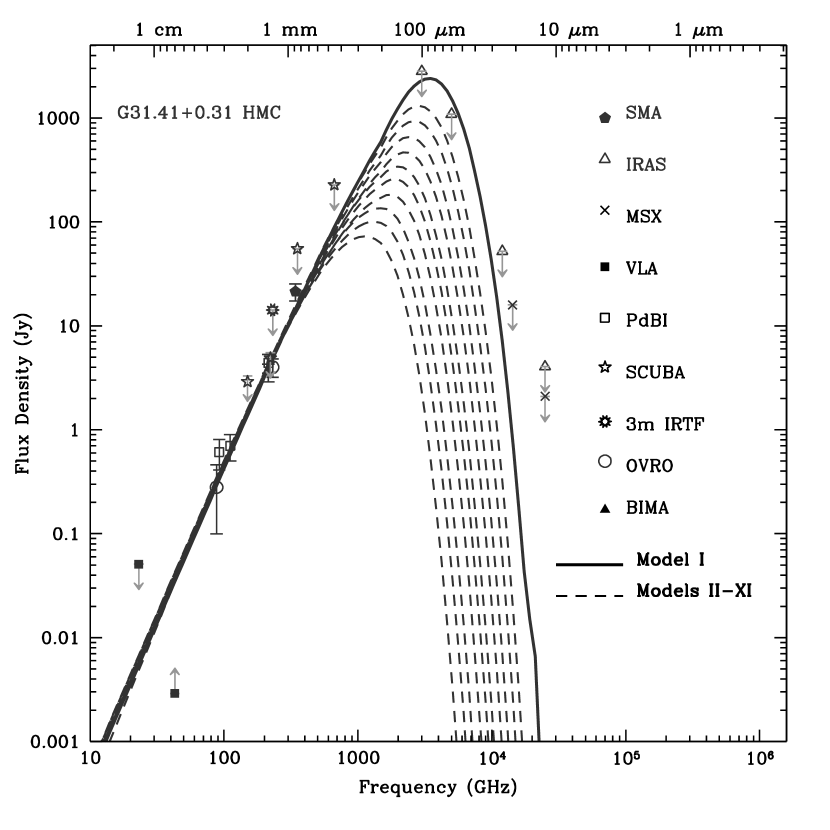
Figure 2: Observed flux densities of G31 HMC (see Table Collapsing Hot Molecular Cores: A Model for the Dust Spectrum and Ammonia Line Emission of the G31.41+0.31 Hot Core) and predicted SED for model I ($M_{*}=25~{}M_{\odot}$; solid line) and models II-XI ($M_{*}$ = 15-1 $M_{\odot}$; dashed lines).

G31 HMC has a database of continuum flux density measurements covering a wide range of wavelengths although, unfortunately, most of the data points were obtained with relatively poor angular resolution and the SED is poorly constrained for $\lambda\leq 850~{}\mu$m. G31 HMC is associated with line transitions from a variety of molecular species, such as HCO⁺, SiO (Maxia et al. 2001), ¹³CO (Olmi et al. 1996), CS (Anglada et al. 1996), H₂S, C¹⁸O (Gibb, Mundy & Wyrowski 2004), and CH₃CN (Beltrán et al. 2005). Particularly interesting is the association of G31 HMC with strong ammonia emission (Churchwell et al. 1990, Cesaroni et al. 1992) whose (4,4) inversion transition has been observed with subarcsecond angular resolution using the VLA (Cesaroni et al. 1998; see their Figs. 2c, 4c, and 9c). This makes G31 HMC one of the few sources where a high signal-to-noise ratio analysis of the spatial variation of the ammonia emission along the core can be carried out. The high intensity of the observed ammonia (4,4) emission, the ratio of the main to satellite lines close to unity, as well as the unusually large line widths indicate extreme physical conditions that suggest that this core is harboring an O type star. Because of this, we chose G31 HMC as a candidate to test the molecular emission predictions of the Osorio’s model for the early stages of the formation of massive stars.

We note that VLA observations at 7 mm (Araya et al. 2003) reveal the presence of a binary system at the center of G31 HMC. However, the model of Osorio et al. (1999) is spherically symmetric, with a single central source of luminosity. This assumption is valid as long as the binary separation ($\sim 0\hbox to0.0pt{.\hss}^{\prime\prime}2$) is much smaller than the observed size of the HMC ($\sim 8^{\prime\prime}$). Likewise, deviations from spherical symmetry either by rotation (disks) or by an intrinsic elongation of the cloud are not considered by Osorio’s model. To test non-spherical models, one must include high angular resolution mid-IR data that would allow to properly constrain parameters such as the degree of flattening of the envelope, the centrifugal radius, or the effect of a disk and/or cavities caused by outflows. This kind of data has been obtained for other HMCs and is highly sensitive to the geometry of the cloud (e.g., De Buizer, Osorio & Calvet 2005). Unfortunately, such observations are not yet available for G31 HMC.

Observations of several molecular tracers reveal, however, the existence of small velocity gradients in G31 HMC that have been interpreted as suggestive of either outflow (Gibb, Wyrowski, & Mundy 2004, Araya et al. 2008) or rotation motions (Beltrán et al. 2005). Sensitive high angular resolution observations are needed to clarify this issue. Despite the possible presence of small velocity gradients, we expect the kinematics of the core to be dominated by the overall infall motions of the envelope. In this work we assume that the spherically symmetric models of Osorio et al. (1999) are adequate to study the dust continuum and molecular line emission of G31 HMC.

The paper is organized as follows. In $\S 2$, we describe the modeling procedure, in $\S 3$ we present the observational data available from the literature, in $\S 4$ we model the dust and ammonia data and we compare our results with the observations, as well as with other modeling attempts of this source reported in the literature. Finally, in $\S 5$ we summarize our conclusions.

2 Modeling

2.1 General Procedure

Following Osorio et al. (1999), we model a HMC as a spherically symmetric envelope of dust and gas that is collapsing onto a recently formed central massive star. An accretion shock is formed at the stellar surface. Thus, the stellar radiation and the accretion luminosity provide the source of heating of the envelope. The temperature of the envelope is a function of the distance to the center. The density, infall velocity, and turbulent velocity dispersion for each point of the envelope are obtained from the solution of the dynamical collapse of the SLS (McLaughlin & Pudritz 1997). The parameters of the SLS model are chosen by calculating the emerging dust emission, assuming a constant dust to gas mass ratio along the envelope, and fitting the observed SED.

Once obtained the physical conditions in the envelope from the fit to the observed SED, the excitation of the ammonia molecule is calculated and the radiative transfer is performed in order to obtain the emerging ammonia spectra for different lines of sight towards the envelope. In these calculations, the gas-phase ammonia abundance, that is a function of radius, is the only free parameter. We consider two simple cases: uniform gas-phase abundance and uniform total ammonia abundance. In the latter case, the ratio of gas to solid phase ammonia as a function of radius is determined by calculating the balance between condensation and sublimation of molecules on dust grains. The gas-phase ammonia abundance is constrained by comparing the ammonia model spectra with the observed spectra towards different positions.

2.2 Physical Structure of the Envelope

For the collapsing envelope, we adopt the density, $\rho_{\rm SLS}(r)$, infall velocity, $v_{\rm SLS}(r)$, and turbulent velocity dispersion, $\sigma_{\rm SLS}(r)$, distributions resulting from the solution of the self-similar collapse of the SLS (Adams, Lizano & Shu 1987, unpublished notes). The SLS has a logatropic pressure, $P=P_{0}\ln(\rho_{\rm SLS}/\rho_{0})$, where $P_{0}$ is a constant that sets the pressure scale, and $\rho_{0}$ is an arbitrary reference density, introduced by Lizano & Shu (1989) to empirically take into account the observed turbulent motions in molecular clouds. The collapse of the SLS has been studied by McLaughlin & Pudritz (1996, 1997; hereafter MP97), and it has been generalized by Reid, Pudritz & Wadsley (2002), and Sigalotti, de Felice & Sira (2002) to include three-dimensional hydrodynamic calculations of the collapse of both singular and nonsingular logatropic spheres.

In the SLS collapse solution an expansion wave moves outward into a static cloud and sets the gas into motion towards the central star. Both the speed of the expansion wave and the mass accretion rate increase with time. The radius of the expansion wave is given by

$$r_{\rm ew}={1\over 4}(2\pi GP_{0})^{1/2}\,t^{2},$$ (1)

where $t$ is the time elapsed since the onset of collapse.

Outside the radius of the expansion wave ($r>r_{\rm ew}$), the SLS envelope is static,

$$v_{\rm SLS}=0,$$ (2)

and the density is given by

$$\rho_{\rm SLS}(r)=(P_{0}/2\pi G)^{1/2}\,r^{-1}.$$ (3)

Inside the expansion wave ($r<r_{\rm ew}$), the infall velocity, whose direction is radial, is given by

$$v_{\rm SLS}(r)={{1}\over{2}}(2\pi GP_{0})^{1/2}t\,u(x),$$ (4)

having a free-fall behavior for $r\ll r_{\rm ew}$. The density is

$$\rho_{\rm SLS}(r)={{2}\over{\pi^{1/2}Gt^{2}}}\alpha(x),$$ (5)

where $x=4(2\pi GP_{0})^{-1/2}\,r\,t^{-2}$ is the similarity variable, and $u(x)$ and $\alpha(x)$ are non-dimensional functions. With this normalization the expansion wave is located at $x=1$. The self-similar variable, and the density and velocity functions are related to those tabulated by McLaughlin & Pudritz (1997) through $x=2^{5/2}x_{\rm MP}$, $\alpha(x)=2^{-3}\alpha_{\rm MP}(x_{\rm MP})$, and $u(x)=2^{3/2}u_{\rm MP}(x_{\rm MP})$, where the subindex “MP” labels the McLaughlin & Pudritz (1997) solution.

As noted by Osorio et al. (1999) the SLS collapse tends to produce massive envelopes, since inside the radius of the expansion wave only 3% of the mass is in the central star, while 97% is in the collapsing envelope.

The velocity dispersion inside the envelope due to turbulent motions is obtained assuming that Alfvén waves in the cloud induce fluid motions with velocity amplitudes, $\delta v_{\rm tur}$, of the order of the wave speed, $\delta v_{\rm tur}\simeq v_{A}=(dP/d\rho_{\rm SLS})^{1/2}=(P_{0}/\rho_{\rm SLS})^{1/2}$, where the magnitude of the magnetic field is $B=(4\pi P_{0})^{1/2}$. For random polarizations and random orientations of the magnetic field in the cloud, the one-dimensional velocity dispersion in the line-of-sight direction is given by

$$\sigma_{\rm SLS}(r)=\left(\frac{1}{3}\frac{P_{0}}{\rho_{\rm SLS}}\right)^{1/2},$$ (6)

where the factor 1/3 comes from averaging over the solid angle the square of the magnetic field projections along the line of sight.

The physical structure of the SLS collapse is characterized by the constant $P_{0}$ and the time elapsed since the onset of collapse, $t$. In terms of familiar variables, this elapsed time is given by

$$t=\frac{4M_{*}}{\dot{M}},$$ (7)

where $\dot{M}$ is the mass accretion rate, and $M_{*}$ is the mass of the central star. $P_{0}$ can be written as

$$P_{0}=\frac{\dot{M}^{8/3}}{(2^{11}\pi^{3}Gm^{2}_{0}M^{6}_{*})^{1/3}},$$ (8)

where $m_{0}=0.0302$ is the reduced (dimensionless) mass. From now on, we will use $M_{*}$ and $\dot{M}$ to characterize the dynamical model.

The total source of heating of the envelope, $L_{\rm tot}$, is assumed to be the sum of the stellar luminosity, $L_{*}$, and the accretion luminosity, $L_{\rm acc}=GM_{*}{\dot{M}}/R_{*}$, where $R_{*}$ is the stellar radius. A value of $R_{*}=1\times 10^{12}$ cm has been adopted (see Osorio et al. 1999, Hosokawa & Omukai 2008). The stellar luminosity is related to the stellar mass using the Schaller et al. (1992) evolutionary tracks. The temperature of the dust grains inside the envelope, $T(r)$, is self-consistently calculated from the total luminosity using the condition of radiative equilibrium for outer optically thin regions of the envelope, whereas for the inner optically thick regions the temperature is calculated from the standard diffusion approximation (see details in Osorio et al. 1999).

For temperatures $\gtrsim 60$ K and densities $\gtrsim 10^{5}$ cm^-3, the gas and dust are well coupled and are described by the same temperature (e.g., Sweitzer 1978; Doty et al. 2002). Our models fulfill this condition and, thus, the kinetic temperature of the gas, $T_{k}$, is taken to coincide with the temperature obtained from the dust calculations, $T_{k}(r)=T(r)$.

Assuming that the dust grains shield the molecules from the intense central radiation field, the dust destruction front, at the dust sublimation temperature ($\sim 1200$ K), determines the inner radius, $R_{\rm dust}$, of the dust and molecular envelope. The external radius, $R_{\rm ext}$, of the envelope is inferred from the observations.

2.3 Dust Continuum Emission

To solve the radiative transfer equation for the dust emission we have the geometry depicted in Figure 1. Given the spherical symmetry of the envelope, the emergent specific intensity, $I_{\nu}$, for a given line of sight is only a function of the impact parameter, $p$, the distance between the line of sight and the center of the envelope. Assuming that the source function of the thermal dust emission is the Planck function evaluated at the dust temperature, $B_{\nu}(T)$, we have the following set of equations that allow us to obtain the emerging intensity as a function of frequency and impact parameter,

$$I_{\nu}(\nu,p)=I_{\rm bg}(\nu)~{}{e}^{-\tau}+\int^{\tau}_{0}B_{\nu}(T)~{}{e}^{-\tau^{\prime}}~{}d\tau^{\prime},$$ (9)

$$\tau^{\prime}(\nu,p,s^{\prime})=\int^{s^{\prime}}_{-s_{0}}\kappa(\nu)\,\rho_{\rm SLS}(s,p)~{}ds,$$

and

$$\tau(\nu,p)=\int^{+s_{0}}_{-s_{0}}\kappa(\nu)\,\rho_{\rm SLS}(s,p)~{}ds,$$

where $I_{\rm bg}(\nu)$ is the background intensity, $\kappa(\nu)$ is the monochromatic dust absorption coefficient per unit mass, $s$ is the coordinate along the line of sight ($r^{2}=p^{2}+s^{2}$), positive in the direction away from the observer, and whose origin is in the plane perpendicular to the line of sight that contains the center of the envelope (see Fig. 1). The integration limits $-s_{0}$ and $+s_{0}$ correspond to the edges of the envelope nearest and farthest to the observer, respectively, being $s_{0}=\sqrt{R^{2}_{\rm ext}-p^{2}}$. In the absence of a strong background source, $I_{\rm bg}$ will be taken as the cosmological background, $I_{\rm bg}=B_{\nu}(T_{\rm bg})$, where $T_{\rm bg}=2.7$ K.

Following Osorio et al. (1999), the dust absorption coefficient, $\kappa(\nu)$, at high frequencies ($\nu>1500$ GHz) is obtained from D’Alessio (1996), who considered spherical (Mie) particles of graphites, silicates, iron, and water ice compounds, with the standard grain-size distribution of the interstellar medium, $N(a)\propto a^{-3.5}$ (Mathis, Rumpl, & Nordsieck 1977), with a minimum radius of 0.005 $\mu$m and a maximum radius of 0.3 $\mu$m. The abundance and optical constants of the compounds were taken from Draine & Lee (1984), Draine (1987), and Warren (1984). The value of the absorption coefficient at 1500 GHz obtained for this dust composition and size distribution can be extrapolated to lower frequencies in the standard power-law form, resulting $\kappa(\nu)=0.06(\nu/{\rm 1500~{}GHz})^{\beta}$ cm² g^-1 for $\nu\leq 1500$ GHz. The value of the index $\beta$ is adopted so that it is consistent with the slope of the optically thin millimeter emission of the observed SED, where $S_{\nu}\propto\nu^{(2+\beta)}$. We assumed a constant dust-to-gas mass ratio of 0.01. Depending of the wavelength, the D’Alessio (1996) opacities can be a factor of up to 2-3 times lower than those of Ossenkopf & Henning (1994). Both opacity models have been successfully used to reproduce the SED of other high mass star forming cores (Osorio et al 1999, van der Tak et al 2000).

Once the emergent intensity as a function of the impact parameter is obtained, the total flux density of the source at a given frequency is calculated as

$$F_{\nu}(\nu)={{2\pi}\over{D^{2}}}\int^{R_{\rm ext}}_{0}I_{\nu}(\nu,p)\,p\,dp,$$ (10)

where $D$ is the distance of the observer to the source. Finally, the resulting model SED is calculated and compared with the observed SED. A grid of models is run with different values of the free parameters $\dot{M}$ and $M_{*}$ (or, equivalently, $L_{*}$). In this way, the model (or models) that are consistent with the observed SED are determined. Note that in case the SED is not well constrained, more than one model can be consistent with the data. Further details on the method are described by Osorio et al. (1999).

2.4 Ammonia Line Emission

In this section, we describe the calculation of the emerging intensity of the ammonia inversion transitions arising from a spherically symmetric envelope with the physical properties obtained from the dust modeling using the SLS solution.

The physics of the ammonia molecule is studied in detail in Townes & Slawlow (1975), Ho (1975), and Ho & Townes (1983). Here we only summarize some basic information that may be relevant to our discussion. Because ammonia is a symmetric top molecule, its rotational energy levels are described by two quantum numbers, namely, the total angular momentum, $J$, and its projection on the symmetry axis, $K$ ($K\leq J$). Rotational levels with $J=K$ are more populated and are called metastable, while rotational levels with $J\neq K$ are short-lived and are called non-metastable. All rotational levels (except those with $K=0$) are split into inversion doublets. The transitions between these inversion doublets are called inversion transitions and occur at wavelengths of $\sim$1.3 cm.

As shown in Appendix A, the excitation temperature of the ammonia inversion transitions can be obtained from a two-level model. For a given point of coordinate $s$ along a line of sight of impact parameter $p$, we can estimate the excitation temperature, $T_{\rm ex}(s,p)$, from equation (A1), taking the total number density of gas molecules as $n(r)=\rho_{\rm SLS}(r)/(\mu_{m}\,m_{\rm H}$), where $\mu_{m}=2.3$ is the mean molecular weight in the envelope and $m_{\rm H}$ is the hydrogen mass. In the calculation of $T_{\rm ex}$ we will approximate the intensity of the local radiation field by the background intensity ($I_{r}(s,p)\simeq I_{\rm bg}$). With this approximation, equation (A1) gives a lower limit for the excitation temperature. However, as shown in Appendix A, for the physical conditions of HMCs the values obtained in this way are very close to the value of the kinetic temperature, which, for thermal lines, is an upper limit for the excitation temperature. Therefore, this indicates that taking $I_{r}=I_{\rm bg}$ is a very good approximation for the calculation of the excitation temperature in HMCs. Note that, with this approximation, the resulting excitation temperature will become a spherically symmetric function, $T_{\rm ex}(r)$.

The spectra of the inversion transitions present a hyperfine structure due to the interaction of the electric quadrupole momentum of the nitrogen nucleus with the electric field of the electrons. This effect splits the line into five components, the central main line, and two pairs of satellite lines, separated $\sim$1-2 MHz, symmetrically placed about the main line. These hyperfine components are further split by weaker magnetic spin interactions. Since the separation between the magnetic hyperfine components is only $\sim$10-40 kHz (0.1-0.5 km s^-1), they are distinguishable only in very high spectral resolution observations of regions with very low velocity dispersion. For this reason, we neglect the magnetic hyperfine structure, and we restrict our analysis to only the five electric quadrupole hyperfine components.

As shown in Appendix B (eq. [B13]), the absorption coefficient of the ammonia $(J,K)$ inversion transition, at a given point of coordinate $s$ along a line of sight of impact parameter $p$ (see Fig. 1), as a function of the observed LSR velocity, $V$, is given by

$$\kappa(V,s,p) = {\left(1\over 128\pi^{3}\right)^{1/2}{c^{3}A_{ul}\over\nu_{0}^{3}}{{\rho_{\rm SLS}(r)X_{\rm NH_{3}}(r)}\over{1.2\mu_{m}m_{\rm H}\sigma_{V}(r)}}{e^{h\nu_{0}/kT_{\rm ex}(r)}-1\over e^{h\nu_{0}/kT_{\rm ex}(r)}+1}}$$ (11)

$$\times{g_{JK}e^{-E_{JK}/kT_{\rm rot}(r)}\over Q(T_{\rm rot}(r))}\sum_{i=1}^{5}x_{i}e^{-\left(V-V_{i}-V_{c}-v_{\rm SLS}(r)\,s/r\right)^{2}/2\sigma_{V}^{2}(r)},$$

where the frequency $\nu_{0}$ corresponds to that of the main line of the inversion transition (given in Table 4), $X_{\rm NH_{3}}(r)$ is the local gas-phase ammonia abundance relative to H₂, $\sigma_{V}(r)$ is the local dispersion of the distribution of line-of-sight velocities due to turbulent and thermal motions, $T_{\rm rot}(r)$ is the local rotational temperature, $g_{JK}$ is the statistical weight of the $(J,K)$ rotational level (given by equation [B7]), $E_{JK}$ its rotational energy (given by equation [B8]), $Q(T_{\rm rot})$ is the partition function (given by equation [B12]), $x_{i}$ is the relative strength of the $i$th hyperfine component ($\sum_{i=1}^{5}x_{i}=1$) and $V_{i}$ its Doppler velocity shift with respect to the main line (both given in Table 5), $V_{c}$ is the LSR velocity of the ambient cloud, and the term $v_{\rm SLS}(r)\,s/r=V_{s}$ is the line-of-sight component of the infall velocity of the envelope. In writing equation (11) it has been assumed that $n=1.2n_{\rm H_{2}}$, corresponding to assume a 10% He abundance. Note that the excitation temperature, $T_{\rm ex}$, and the Einstein spontaneous emission coefficient, $A_{ul}$, are those of the entire inversion transition, unsplit by hyperfine interactions (eq. [A1] and Table 4, respectively). Due to the dipolar selection rules on the rotational transitions, the populations of the metastable levels are mainly determined by collisions; therefore, $T_{\rm rot}$, that is defined by the relative populations of the rotational levels is expected to be similar to the kinetic temperature. In fact, $T_{\rm rot}$ is a lower limit of $T_{k}$, and its value is different for each pair of rotational levels considered (see Appendix B). However, the agreement between $T_{\rm rot}$ and $T_{k}$ is expected to improve for high metastable levels, due to the increased excitation involved, and for high densities, where all temperatures tend to thermalize to $T_{k}$ (e.g., Walmsley & Ungerechts 1983; Danby et al. 1988; Wilson et al. 2006). This is the case for G31 HMC (Osorio 2000), and hereafter we will take $T_{\rm rot}$=$T_{k}$.

In the above equation, the dispersion of the line-of-sight velocity distribution results from the contribution of the macroscopic (turbulent) and microscopic (thermal) components,

$$\sigma_{V}(r)=\sqrt{\sigma^{2}_{\rm SLS}(r)+\sigma^{2}_{\rm th}(r)},$$ (12)

where $\sigma_{\rm SLS}(r)$ is given by equation (6) and $\sigma_{\rm th}(r)$ is given by

$$\sigma_{\rm th}(r)={{kT_{k}(r)}\overwithdelims( ){m_{\rm NH_{3}}}}^{1/2},$$ (13)

where $m_{\rm NH_{3}}$ is the mass of the ammonia molecule.

The only free parameter in equation (11) is the gas-phase ammonia abundance, $X_{\rm NH_{3}}(r)$. The smallest values of the ammonia abundance reported in the literature are found in the coolest cores of low-mass star forming regions, with typical abundances of $X_{\rm NH_{3}}=10^{-8}$-$10^{-7}$ (e.g., Herbst & Klemperer 1973, Ungerechts et al. 1980, Estalella et al. 1993), and some chemical models predict abundances as low as $X_{\rm NH_{3}}=10^{-10}$-$10^{-9}$ (Le Bourlot et al. 1993). The highest values, obtained in very hot regions of massive star formation (e.g., Millar 1997, Walmsley 1997, Ohishi 1997), are $X_{\rm NH_{3}}=10^{-6}$-$10^{-5}$.

Neglecting chemical effects, we consider the two simplest possibilities for the function, $X_{\rm NH_{3}}(r)$, that describes the gas-phase ammonia abundance inside the envelope. First, we consider the case in which $X_{\rm NH_{3}}(r)$ has a constant value across the envelope. As a second possibility, we consider the case in which the total (solid+gas) ammonia abundance remains constant across the envelope but the gas-phase abundance increases towards the center because of the temperature gradient. Variations in the gas-phase molecular abundances have already been explored by, e.g., van der Tak et al. (2000), and Boonman et al. (2003) to explain the CH₃OH, HCN, and H₂O emission in some regions of massive star formation. We assume a minimum gas-phase ammonia abundance, $X_{\rm min}$, in the outer, cooler parts of the core, where the bulk of the ammonia molecules are frozen in grain mantles. The ammonia molecules are released from the grain mantles to the gas phase, reaching a maximum value of the gas-phase ammonia abundance, $X_{\rm max}$, in the inner, hotter regions of the core, where it is assumed that all the ammonia molecules are in the gas phase. Under this simple approximation, the gas-phase ammonia abundance as a function of the distance to the center of the core will be given by

$$X_{\rm NH_{3}}(r)={{X_{\rm max}-X_{\rm min}}\over{1+\eta(n(r),T(r))}}+X_{\rm min},$$ (14)

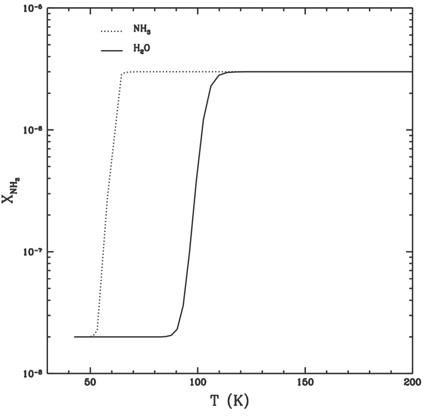
Figure 8: Gas-phase ammonia abundance as a function of temperature, obtained from the balance between the condensation and sublimation of molecules on dust grains following the thermal equilibrium equation of Sandford and Allamandola (1993) (see text). The dotted line corresponds to the sublimation of pure ammonia molecules, while the solid line corresponds to the assumption that ammonia molecules are trapped in water ice mantles, being released to the gas phase after sublimation of water molecules. For this temperature range, the results depend weakly on the density, for which the density distribution field of G31 HMC has been assumed.

where $\eta(n,T)$ is the ratio between the solid and gas phases, obtained from the balance between the condensation and sublimation of molecules on dust grains following the thermal equilibrium equation of Sandford & Allamandola (1993) (see Appendix C). Two possible cases are considered. First, it is assumed that the ammonia molecules are directly frozen in grain mantles, with $\eta(n,T)$ described by equation (C4); in this case, the ammonia molecules are released to the gas phase at the ammonia sublimation temperature, which is of $\sim$60 K for the range of densities typical in HMCs (see Fig. 8). As a second possibility, it is assumed that the ammonia molecules are trapped in water ice, being released to the gas phase only after sublimation of water molecules, that occurs at a temperature of $\sim$100 K as described by equation (C5) (see Fig. 8).

As in the case of the continuum emission ($\S$ 2.3), we adopt the geometry of Figure 1, and the emergent specific intensity, $I_{\nu}$, will be given by

$$I_{\nu}(V,p) = I_{\rm bg}~{}{e}^{-\tau}+\int^{\tau}_{0}B_{\nu}(T_{\rm ex}(s,p))~{}{e}^{-\tau^{\prime}}~{}d\tau^{\prime},$$ (15)

$$\tau^{\prime}(V,p,s^{\prime})=\int^{s^{\prime}}_{-s_{0}}\kappa(V,s,p)~{}ds,$$

$$\tau(V,p)=\int^{+s_{0}}_{-s_{0}}\kappa(V,s,p)~{}ds,$$

where $T_{\rm ex}$ is given by equation (A1), and $\kappa(V,s)$ is given by equation (11). As for the dust calculations, in the absence of a strong background source, the background intensity will be taken as the cosmological background, $I_{\rm bg}=B_{\nu}(T_{\rm bg})$, where $T_{\rm bg}=2.7$ K. The geometrical parameters are the same as in equation (9).

Finally, in order to make an accurate comparison with the observations, the emergent intensity is convolved (in 2-D) with a Gaussian with a FWHM equal to that of the observing beam, and a velocity smoothing is applied to reproduce the spectral resolution of the spectrometer. Note that $X_{\rm min}$ and $X_{\rm max}$ are the only parameters to be fitted by the molecular line modeling.

3 The Data

Numerous observations of the G31.41+0.31 region are reported in the literature. The main results of the continuum flux density measurements in the wavelength range $\sim 10~{}\mu$m to 1.3 cm are summarized in Table Collapsing Hot Molecular Cores: A Model for the Dust Spectrum and Ammonia Line Emission of the G31.41+0.31 Hot Core. Most of these observations did not have the angular resolution required to separate the emission of the HMC from that of the G31.41+0.31 UCHII region, whose emission peak is only $\sim 5^{\prime\prime}$ apart. Thus, it is likely that in the data obtained with angular resolution $>5^{\prime\prime}$ the dust continuum emission of the HMC is contaminated by emission originated in the nearby UCHII. Therefore, we have considered these data as upper limits. In addition, we note that the flux density at 1.3 cm is likely dominated by free-free emission. Then, we expect the dust thermal emission at this wavelength to be well below the upper limit set by the observations, and therefore, in our modeling, we did not attempt to reproduce the emission at 1.3 cm and longer wavelengths. Finally, we considered the 7 mm data point as a lower limit since it is likely that a fraction of the flux density is missed in the very high angular resolution interferometric VLA observations at this wavelength.

Observations of several line transitions from a variety of molecular species have been carried out towards G31 HMC. Among them, the VLA B-array observations of the NH₃ (4,4) inversion transition (VLA project code AH0483) reported by Cesaroni et al. (1998) (combined with C-array data from Cesaroni et al. 1994) constitute one of the best sets of high angular resolution data towards G31 HMC and objects of the same kind published so far. These combined data have an angular resolution of $0\farcs 63$ (corresponding to a spatial scale of 5000 AU at the distance of 7.9 kpc of the source), high enough to spatially resolve the structure of the core, revealing its extreme physical conditions and their variation inside the core. Thus, we used this dataset to carry out the main part of our spectral line data analysis.

Figure 9c of Cesaroni et al. (1998) shows the ammonia (4,4) spectra as a function of the impact parameter with respect to the center of G31 HMC. As can be seen in the figure, the brightness temperature is very high, reaching a value of approximately 100 K for the line-of-sight towards the center of the core, indicating high values of the kinetic temperature. The optical depth is also high, as indicated by the fact that the satellite lines, whose opacity is $\sim$1/60 that of the main line, reach an intensity similar to that of the main line towards the center of the core. Also, lines are unusually broad, resulting in the blending of contiguous satellite lines, indicative of large turbulent motions. This figure also indicates that the physical conditions in the core change as a function of the distance to the center, as shown by the variation of the line intensity and ratio between main line and satellites for different impact parameters.

In addition to the subarcsecond resolution ammonia data of Cesaroni et al. (1998), Churchwell et al. (1990) and Cesaroni et al. (1992) report a multitransitional ammonia study of G31 HMC carried out with the Effelsberg 100 m telescope. These observations have an angular resolution of $40^{\prime\prime}$. Although the study lacks the angular resolution to be sensitive to variations of the line parameters across the core, providing only the integrated ammonia emission of the overall core, these data are useful to further test the model predictions derived from the analysis of the dust and high angular resolution ammonia (4,4) line data.

In the next section we present a simultaneous analysis of the dust continuum and ammonia line data that will provide a powerful diagnostic to constrain the physical conditions inside G31 HMC.

4 Comparison of the Model with the Observations

4.1 Dust Continuum Emission

The observed SED of G31 HMC is characterized by strong millimeter emission suggesting the presence of either a hot or a dense envelope (or a combination of both). Therefore, “a priori” we expect the models that are able to fit the observed SED to be characterized by a high mass accretion rate. Bearing this in mind, we ran a grid of models covering a relatively wide range of values of the free parameters $M_{*}$ and $\dot{M}$. The mass and luminosity of the central star have been related using the evolutionary tracks of Schaller et al. (1992) for a solar metallicity. We tested the same values of the mass given in the tables of Schaller et al. in the range $1~{}M_{\odot}\leq M_{*}\leq 40~{}M_{\odot}$ (corresponding to $0.7~{}L_{\odot}\leq L_{*}\leq 2\times 10^{5}~{}L_{\odot}$), and for the mass accretion rate we explored the range $10^{-5}~{}M_{\odot}~{}{\rm yr^{-1}}\leq{\dot{M}}\leq 10^{-2}~{}M_{\odot}~{}{\rm yr^{-1}}$. We set the value of $\beta$ so that the slope of the model SED was consistent with that of the observed SED in the millimeter wavelength range, resulting in values of $\beta$ in the range 1-1.2. We set the external radius to $R_{\rm ext}$ = 30,000 AU, a value inferred from the observed images of the source (e.g., Cesaroni et al. 1994a, Maxia et al. 2001) and required to reproduce the large flux densities observed in the millimeter range.

Because of the incompleteness of the observed SED of G31 HMC, there is more than one model that can fit the available observational data. In Table 2 we give the parameters of a set of models (corresponding to values of the stellar mass listed in the tables of Schaller et al. 1992) that are consistent with the observed SED. The higher luminosity (and hotter envelope) model consistent with the observed SED has a central star with a mass of $M_{*}=25~{}M_{\odot}$ and an accretion rate of $\dot{M}=2.6\times 10^{-3}~{}M_{\odot}~{}{\rm yr}^{-1}$. Models with $M_{*}>25~{}M_{\odot}$ produce far- and mid-IR flux densities that exceed the observational constraints. Lower luminosity models ($M_{*}<25~{}M_{\odot}$) that are consistent with the SED data have colder envelopes, but they have a higher density (see the values of the temperature and density at $r=1000$ AU listed in the table) in order to account for the strong millimeter emission observed in G31 HMC, resulting in higher values for the mass of the envelope. Note that a low value of $M_{*}$ does not imply that the source is a low-mass protostar since in Table 2 the models with the smaller central mass are also the younger sources, meaning simply that the time elapsed since the onset of collapse, $t$, is still too short to accumulate a massive central object. In fact, as can be seen in the table, these models are associated with the more massive envelopes and would eventually form the higher mass stars.

The value of the inner radius of the envelope, $R_{\rm dust}$, is $\sim 156$ AU for model I ($M_{*}=25~{}M_{\odot}$) and gets smaller as the mass of the central star decreases. We note that in all these models the radius of the expansion wave, $r_{\rm ew}$, is smaller than the radius of the core, $R_{\rm ext}$; therefore, the outermost regions of these envelopes are static. Also, the infall accretion rates in these models are so high that the accretion luminosity is the most important source of energy. For a given value of $M_{*}$, the observational uncertainties in the SED data points result in a variation of $\sim 10\%$ in the possible values of $\dot{M}$ that are consistent with the data. This results also in a formal uncertainty of the order of 10% in the derived parameters listed in Table 2 for a given value of $M_{*}$.

Figure 3 shows the physical structure of the SLS envelopes corresponding to the models listed in Table 2. As the figure illustrates, model I has the higher values of the velocity and temperature, and the lower values of the density and velocity dispersion. Turbulent motions are the most important contributors to the local velocity dispersion at large radii of the envelope, reaching values of $\sigma_{\rm SLS}>4$ km s^-1 in the outermost regions.

4.2 Ammonia (4,4) Line Emission

Here we obtain the NH₃ emission for the models that are consistent with the observed SED of G31 HMC to further test their physical properties by comparing their emission with the VLA observations of the NH₃(4,4) inversion transition reported by Cesaroni et al. (1998). In order to reproduce the setup of the Cesaroni et al. observations, the emerging ammonia intensity as a function of the LSR velocity, $V$, is calculated for each line of sight through the core and convolved with a Gaussian beam of HPBW = $0\farcs 63$. The spectra have been converted into a brightness temperature scale using the relation $T_{B}=2.1(F_{\nu}/\rm mJy~{}beam^{-1})(HPBW/arcsec)^{-2}$. A velocity range of $\sim$ 150 km s^-1 is covered, and Hanning smoothing is applied to obtain an effective spectral resolution of 4.86 km s^-1. A value of $V_{c}=97.4$ km s^-1 has been adopted for the LSR velocity of the ambient cloud. Figure 9c of Cesaroni et al. (1998) shows the spectra obtained by averaging the observed ammonia emission over circular annuli around the position of the core center. Therefore, in order to make more accurate the comparison of the model results with the observations, the spectra have been calculated for the impact parameters $p$ = 0, 5000, 10000, and 15000 AU, corresponding to the values sampled in this figure.

4.2.1 Constant Gas-Phase Ammonia Abundance

We first ran a grid of cases with different values of the gas-phase ammonia abundance, assumed to be constant along the envelope. We tested a wide range of values, from $X_{\rm NH_{3}}=10^{-9}$ to $X_{\rm NH_{3}}=10^{-5}$, for all the models resulting from the fit to the observed SED (discussed in $\S$ 4.1). After running all these cases, we conclude that none of these models is able to reproduce the observed spectra.

Figure 4 shows the synthetic spectra obtained for model I at different impact parameters and for different ammonia abundances. The spectra observed by Cesaroni et al. (1998) are also shown for comparison. This figure shows that model I cannot reproduce the observed behavior of the ammonia emission as a function of impact parameter. For a low ammonia abundance (left column), the main line reaches the observed brightness temperature of $\sim 100$ K in the $p=0$ panel; however, the satellite lines are too weak in all the panels. Increasing the ammonia abundance (middle and right columns) produces an increase of the intensity of the satellite lines, that reach a value close to the observed one ($\sim 100$ K) in the $p$ = 0 AU panel of the right column. Nevertheless, in this panel the main line reaches a brightness temperature of only $\sim 40$ K, which is much smaller than the observed value. This occurs because the main line is very optically thick (reaching an opacity of $\tau_{\rm main}\simeq 350$) and, thus, the brightness temperature must be roughly equal to the kinetic temperature of the outer parts of the envelope model, which are cold. Note that the brightness temperature of the satellite lines is higher since their opacity is 60 times lower, and they can reach the inner parts of the envelope where the temperatures are higher.

Models II to XI are colder than model I (see Fig. 3) and therefore, they are worse in reproducing the observed behavior of the ammonia emission. As for model I, for a low abundance the satellite lines are too weak in all the panels. The intensity of the satellite lines increases with the ammonia abundance but, as in model I, for high ammonia abundances the main line becomes very optically thick in the $p$ = 0 AU panels ($\tau_{\rm main}>380$) and only traces cold material from the outer envelope. Since models II to XI are colder than model I, the line intensities are lower and remain well below the observed values.

Clearly, there is no hope to reproduce the observations with constant values of the ammonia abundance. A high optical depth is required to reproduce the intense satellite lines, but this high opacity prevents that the main line is formed in the inner, hottest regions resulting in a main line brightness temperature too low. Nevertheless, the analysis of constant abundance suggests the alternative of having a low abundance in the outer envelope and a high abundance in the inner parts. In this way, the colder, outer parts of the envelope would have a smaller contribution to the observed emission, that would instead trace inner, higher temperatures. One expects that a compromise could be reached, in which the ammonia abundance in the outer parts of the envelope is low enough for the main line not to be saturated until reaching the inner, hotter regions, where the abundance may be high enough for even the satellite lines to become optically thick. In addition, having a low abundance in the outer parts of the envelope would prevent the main line to become saturated in the outer panels, helping to explain the observed decrease of the intensity of the main line as the impact parameter increases.

4.2.2 Variable Gas-Phase Ammonia Abundance

The rationale for a variable ammonia abundance is provided by the calculation of the sublimation of molecules from dust grain mantles (see Appendix C). Given the temperature gradient in the envelope, the outer parts have temperatures below that of sublimation of grain mantles and it is expected that most of the ammonia molecules are trapped there. The ammonia gas-phase abundance should increase drastically in the inner regions of the envelope, where the kinetic temperature reaches the sublimation temperature of the mantles and the ammonia molecules are released to the gas phase. Therefore, inclusion of the process of sublimation of ammonia molecules from grain mantles should provide a more realistic description of the abundance distribution required in the calculation of the ammonia emission.

In order to try to fit the observed ammonia emission using a variable gas-phase ammonia abundance, we first ran a grid of cases with the ammonia abundance calculated using equation (14), and with the ratio, $\eta$, between the solid and gas phases given by equation (C4) of Appendix C (that corresponds to direct sublimation of NH₃ ices). This procedure assumes that most of the ammonia molecules are frozen into grain mantles in the outer parts of the envelope, being released to the gas phase at the ammonia sublimation temperature (about 60 K; see Appendix C and Fig. 8). In this way, the gas-phase ammonia abundance behaves like a step function, with a minimum value, $X_{\rm min}$, in the external parts of the envelope (where the temperature remains below the ammonia sublimation temperature), and increasing steeply to its maximum value, $X_{\rm max}$, for points inside the radius where the ammonia sublimation temperature is reached.

We have explored values for the outer gas-phase NH₃ abundance in the range $10^{-10}\lesssim X_{\rm min}\lesssim 5\times 10^{-7}$, and in the range $10^{-8}\lesssim X_{\rm max}\lesssim 10^{-4}$ for the inner gas-phase NH₃ abundance. However, none of the models resulting from the fit to the observed SED ($\S$ 4.1) is able to reproduce reasonably well the NH₃(4,4) observations. The main problem is that the maximum brightness temperatures of the main line obtained with this kind of ammonia abundance distribution are too low ($\sim 60$ K), to account for the peak brightness temperatures of $\sim 100$ K observed in G31 HMC. Apparently, this occurs because the main line becomes optically thick in regions with temperatures of the order of 60 K, the temperature at which the bulk of ammonia molecules that were frozen in grain mantles are released to the gas phase. Thus, the difficulties to fit simultaneously the main and satellite lines are similar to those of the case of a constant gas-phase ammonia abundance.

As already mentioned, an alternative scenario is that ammonia molecules are mixed with water ice in grain mantles (as suggested, e.g., by A’Hearn et al. 1987 for comets, and by Brown et al. 1988 and Osorio 2000 for HMCs). In this case, ammonia molecules will be trapped in the grain mantles until temperatures high enough for sublimation of water molecules are reached. Therefore, the gas-phase ammonia abundance will be described by equation (14), where $\eta$ corresponds now to the water sublimation and is given by equation (C5) of Appendix C. As illustrated in Figure 8, the transition from low to high gas-phase ammonia abundance occurs at a higher temperature ($\sim 100$ K) than in the case of pure ammonia sublimation. As a result, optically thick lines will trace hotter regions of the envelope, resulting in higher brightness temperatures.

As in the case of pure ammonia sublimation we ran a grid of cases with values for the outer gas-phase NH₃ abundance in the range $10^{-10}\lesssim X_{\rm min}\lesssim 5\times 10^{-7}$, and in the range $10^{-8}\lesssim X_{\rm max}\lesssim 10^{-4}$ for the inner gas-phase NH₃ abundance. We found that models II to XI cannot fit the NH₃ observations. The envelopes of the lower luminosity models ($M_{*}\leq 15~{}M_{\odot}$) are apparently too cold to fit the observed spectra. For these models the sublimation temperature of 100 K is reached at a radius $<5000$ AU (see Fig. 3), and therefore the spectra calculated for the outer impact parameters ($p\geq 5000$ AU) behave very much like a case of constant gas-phase ammonia abundance equal to $X_{\rm min}$ (since the lines of sight for $p>5000$ AU only cross the outer regions of the envelope, whose temperatures remain below the sublimation temperature). Since models II to XI could not reproduce the observed spectra with a constant abundance, it is not expected that these models can fit the spectra in the outer panels, even with a variable gas-phase ammonia abundance. In summary, models with $M_{*}\leq 15~{}M_{\odot}$ are too cold to reproduce the observed properties of the NH₃(4,4) spectra, even with a variable gas-phase NH₃ abundance.

In contrast, we have been able to obtain a fairly good fit to the observed spectra using model I ($M_{*}=25~{}M_{\odot}$). In Figure 5 (central column) we show our best fit spectra, obtained using this model with a value of $X_{\rm min}=2\times 10^{-8}$ and a value of $X_{\rm max}=3\times 10^{-6}$. This set of parameters reproduces quite well the observed spectra. It reproduces the observed intensity ($\sim 110$ K) of the main line towards the center of the core ($p=0$), as well as the variation of its intensity as $p$ increases. It also reproduces the observed intensity of the satellite lines in the $p=0$ and $p=5000$ AU spectra. In the $p=10000$ and $p=15000$ AU spectra the observed intensity of the satellite lines is somewhat stronger than predicted, but its signal-to-noise ratio is poor and therefore we consider this discrepancy less significant. Lines are broad (note that the satellite lines on each side of the main line appear blended), and the model also reproduces quite well the observed line widths ($\sim 12$ km s^-1). Interestingly, the best fit is obtained with values of the abundance for the cold and hot parts of the envelope that coincide respectively with the typical values inferred (usually assuming a constant abundance) from the observations of low mass (cold) and high mass (hot) star-forming cores (see $\S$ 2.4), giving additional support to the goodness of the fit.

We also show in Figure 5 two additional cases, corresponding to a lower value of the abundance in the hot region of the envelope, $X_{\rm max}=3\times 10^{-7}$ (left column), and to a higher value of the abundance in the cold region, $X_{\rm min}=2\times 10^{-7}$ (right column), to illustrate the behavior of the resulting spectra when varying these parameters. As Figure 5 illustrates, the satellite lines are mainly sensitive to variations in $X_{\rm max}$ (left and middle columns), whereas the main line is sensitive to variations in $X_{\rm min}$ (middle and right columns). At large values of $p$ ($p$ = 10000 and 15000 AU), the spectra do not change by varying $X_{\rm max}$ because the temperatures along these lines of sight are lower than 100 K and, therefore, sublimation will not occur. Figure 5 (left column) also shows that an abundance of $X_{\rm max}=3\times 10^{-7}$ (ten times lower than in the best fit) in the inner regions of the envelope is high enough to reproduce the observed brightness temperature of the main line, but it is too low to reproduce the satellite lines. On the other hand, as the right column shows, an abundance of $X_{\rm min}=2\times 10^{-7}$ in the outer parts of the envelope (ten times higher than in the best fit model) is adequate to reproduce the brightness temperature of the satellite lines, but not for the main line, whose peak brightness temperature decreases to a value below the observed one. This is because for such a high value of $X_{\rm min}$ the main line becomes very optically thick and the observed emission originates in the outer (and, therefore, colder) regions of the core.

Since the spacing between values of $M_{*}$ listed in Table 2, that correspond to those given by Schaller et al. (1992), is too coarse, especially in the high mass range, we explored additional cases obtaining the relationship between $M_{*}$ and $L_{*}$ by interpolation of the tables of Schaller et al. In this way, we performed a fine tuning of the mass of the central star and determined the range of values of the parameters that is consistent with the observational uncertainties of the data. The results are summarized in Table 3. In summary, the dust continuum SED and the spatial variation of the ammonia spectra can be explained by a dense envelope with a central massive star of mass $M_{*}$ = 20-25 $M_{\odot}$, undergoing an intense accretion at a rate $\dot{M}$ = 2-3 $\times~{}10^{-3}~{}M_{\odot}~{}{\rm yr}^{-1}$, and with a total luminosity of $L_{\rm tot}\simeq 2\times 10^{5}~{}L_{\odot}$. The mass of the envelope is $M_{\rm env}$ = 1400-1800 $M_{\odot}$ and it has a considerable static region that surrounds the collapsing region. The value of the magnetic field is $B$ = 5-6 mG. The outermost region has a velocity dispersion of $\sigma_{\rm SLS}\simeq 4$ km s^-1, dominated by turbulent motions. The temperature of the envelope ranges from $\sim 40$ K (at $r=30,000$ AU) to $\sim 1200$ K (at $r$ = 130-160 AU). The gas-phase ammonia abundance inside the envelope is described by a step-like function with a minimum value of 1-4 $\times 10^{-8}$ in the outer, colder ($<100$ K) region, and 2-4 $\times 10^{-6}$ in the inner, hotter ($>100$ K) region. This distribution of the gas-phase ammonia abundance results from the sublimation of ammonia molecules trapped in water ice grain mantles. The minimum and maximum values of the ammonia abundance are similar to the typical values reported in low and high mass protostellar cores, respectively.

Our results for G31 HMC can be compared with the calculations for this source made by other authors. Cesaroni et al. (1998) carried out an analysis of the NH₃(4,4) main line assuming local thermodynamic equilibrium and that the line is optically thick. They claimed that the observed gradient in the peak brightness temperature is a good estimate of the radial distribution of the kinetic temperature of the gas inside the core. Since the observed peak brightness temperature profile of G31 HMC does not coincide with the expected kinetic temperature profile of a sphere, these authors concluded that neither a collapsing nor an expanding spherical envelope can explain the properties of the observed emission. This conclusion was based on a large velocity gradient (LVG) hypothesis, that implies that for any line of sight with $p\neq 0$ the only contribution to the peak brightness temperature (at zero velocity relative to the ambient cloud) arises from the plane perpendicular to the line of sight that contains the center of the core (since the line-of-sight component of the infall velocity of this material is strictly zero). However, if lines are broad (as is the case in G31 HMC), the LVG hypothesis is not valid since material from outside this plane can also contribute to the emission at the center of the line. Furthermore, if the envelope has a static region (as suggested by our analysis) the peak brightness temperature would have a significant contribution from the material in this static region. Therefore, this analysis does not seem adequate to infer the radial temperature distribution in the envelope and, consequently, the possibility of a collapsing spherical envelope cannot be discarded.

Cesaroni et al. (1998) favored a geometrically thin disk seen almost face on (therefore, with a single temperature for each line of sight) to account for the G31 HMC NH₃(4,4) emission. However, in order to reach a very high optical depth with such a geometrically thin disk a very high surface density would be required. This hypothesis was not tested by Cesaroni et al. (1998), and it is unclear if could correspond to a realistic scenario. Also, the satellite lines were not considered in the analysis, and it is also unclear how the observed variation of the main line to satellites ratio as a function of impact parameter can be reproduced.

Therefore, we conclude that although we followed a simplified approach (a spherically symmetric model with a single central source of luminosity), ignoring deviations from spherical symmetry produced either by rotation (disks) or due to the intrinsic elongation of the cloud, our model accounts for some of the basic observed properties of G31 HMC, especially the highest angular resolution line observations, and constitutes a step ahead in modeling these structures.

4.3 Other Ammonia Transitions

To further test our modeling, we calculated the emerging emission for ammonia transitions other than the (4,4) using the same SLS model and ammonia abundances derived by fitting both the SED and the subarcsecond resolution ammonia (4,4) transition data (Table 3). Unfortunately, for ammonia transitions other than the (4,4) only single-dish data (Churchwell et al. 1990, Cesaroni et al. 1992) are available in the literature. These observations were obtained with the 100 m telescope, with an angular resolution of $40^{\prime\prime}$. Therefore, a convolution of the model results with a Gaussian with a FWHM=$40^{\prime\prime}$ was performed. Since this angular resolution is insufficient to resolve the emission of the core, only the spectra towards the $p=0$ position have been calculated. A value of $V_{c}=97.4$ km s^-1 has been adopted for the LSR velocity of the ambient cloud.

In Figure 6 we show the model spectra for the (1,1), (2,2), (4,4), and (5,5) transitions overlaid on the spectra observed by Churchwell et al. (1990) and Cesaroni et al. (1992). The uncertainty in the absolute calibration of the observed spectra is estimated to be about 30% (Churchwell et al. 1990, Cesaroni et al. 1992). As can be seen in the figure, the model spectrum of the (4,4) line coincides pretty well (within $\sim$10%) with the observed one. For the (2,2) and (5,5) lines, the brightness temperatures of the model spectra are $\sim 30$% lower than in the observed spectra, which is still within the calibration uncertainties. The ratio of intensities of the main to satellite lines, which is independent of the calibration, is $\sim 3.5\pm 0.9$ for the observed (2,2) spectrum (the uncertainty in the ratio is estimated from the rms of the spectrum), in agreement with the value of 3.9 obtained for the model spectrum. The ratio is $\sim 3\pm 0.8$ for the observed (5,5) spectrum, which is also in agreement with the value of 3.5 obtained for the model spectrum. The observed line width (FWHM) of the (2,2) main line is $\sim 6$ km s^-1, somewhat smaller than the value of $\sim 10$ km s^-1 obtained for the model spectrum. Finally, the observed line width of the (5,5) main line is $\sim 9$ km s^-1, which is very similar to the value of $\sim 10$ km s^-1 predicted by the model. Given the coincidence of line ratios and line widths, and taking into account the uncertainty in the calibration, we consider that the model predictions are roughly consistent with the observations of the (2,2), (4,4), and (5,5) transitions. However, uncertainties in the calibration are large (30%) and a definitive conclusion is difficult to attain with the present data. For the ammonia (1,1) line, the brightness temperature of the model spectrum is significantly lower than that of the observed spectrum, and the shape of the spectrum is also different. We believe that for the ammonia (1,1) transition, that traces the colder gas, there is likely a significant contribution of cold molecular gas from outside the core (see Hatchell et al. 2000), which is not considered in our modeling. Also, the assumption $T_{\rm rot}$=$T_{k}$ used in deriving our ammonia spectra could affect these results.

We conclude that our model parameters, obtained by fitting the dust and high angular resolution NH₃(4,4) transition data, can also reproduce, within the observational uncertainties, the intensities, line profiles, and main to satellite line ratios of the multitransitional ammonia data. Our modeling is carried out by fitting essentially four parameters, namely, the mass accretion rate and the mass of the central star (or, alternatively, the stellar luminosity) in a physically self-consistent collapse model of a SLS envelope, and the minimum and maximum gas-phase ammonia abundances inside this envelope. We conclude therefore that in massive protostars, where an important temperature gradient is expected to be present, an analysis in terms of a realistic, self-consistent model that takes into account the gradients in the physical properties inside the core is necessary to properly interpret the observational data.

The modeling we carried out for G31 HMC, including the continuum SED as well as the high angular resolution properties of the molecular emission, is, to our knowledge, one of the more complete ever made for a hot molecular core. This source appears to be a good laboratory to test the very early stages of massive star formation.

5 Summary and Conclusions

Our main results can be summarized as follows:

1. We have succeeded in developing a self-consistent model of the physical structure of a hot core, described as a spherically symmetric SLS envelope infalling onto a massive star. The model predicts the continuum emission SED as well as the shape and intensity of ammonia lines.

2. This model is able to reproduce the general observed properties of G31 HMC. In addition to the SED, it can reproduce the strong intensity of the main and satellite ammonia (4,4) lines, as well as their spatial variations as observed with subarcsecond angular resolution. The same model can roughly reproduce, within the observational uncertainties, the single-dish ammonia (2,2), (4,4), and (5,5) data. The ammonia (1,1) data likely have a significant contribution of cold gas outside the core that has not been included in the model.

3. Although the SED fitting alone cannot constrain adequately the parameters of G31 HMC, the simultaneous fitting of the SED and the ammonia emission allows us to obtain a preliminary estimate of the physical parameters of this source. Our best fit model for G31 HMC has a central protostar of 20-25 $M_{\odot}$, with an age of 3-4 $\times 10^{4}$ yr, a high mass accretion rate of 2-3 $\times 10^{-3}~{}M_{\odot}$ yr^-1, and a total luminosity of $\sim 2\times 10^{5}~{}L_{\odot}$. The magnetic field is 5-6 mG. The mass of the envelope is large, 1400-1800 $M_{\odot}$, and its temperature is high, ranging from $\sim 40$ K at the outer radius of the envelope (30,0000 AU) to $\sim 1200$ K at the inner radius (130-160 AU).

   A steep increase of the gas-phase ammonia abundance, from $\sim 2\times 10^{-8}$ in the outer parts of the envelope to $\sim 3\times 10^{-6}$ in the inner parts, is required to reproduce the observed spatial variations of the high angular resolution ammonia spectra. This is naturally explained as a result of the release (at a characteristic temperature of $\sim 100$ K) of ammonia molecules trapped in water ice grain mantles. Therefore, taking into account variations in the gas-phase molecular abundances because of sublimation and freezing-out of molecules onto grain surfaces appears to be necessary to properly reproduce the highest angular resolution observations, and will probably be a key ingredient in the modeling of future line observations with ALMA.

4. Although the actual scenario for G31 HMC is certainly complex (binaries, rotation, outflows, …), our simple model can provide a rough description of the main features of the star formation process in this source, revealing that massive protostars appear to be able to excite high excitation ammonia transitions, not only at circumstellar scales, but also in the larger scale ($\sim$ 30,000 AU) infalling envelopes.

   However, the SED of G31 HMC is still incomplete, lacking high angular resolution data at wavelengths shorter than 880 $\mu$m. Also, high angular resolution line data are only available for the ammonia (4,4) transition, and the calibration uncertainties in the lower angular resolution observations of other transitions are still too large to properly constrain the models. Higher quality data as well as an improved modeling would be necessary to make firm statements on the physical properties of this source.

Appendix A Excitation Temperature of the Ammonia Inversion Transitions

Since the inversion transitions inside a given rotational level of the ammonia molecule are more frequent than the transitions to other rotational levels, we approximate any metastable inversion doublet by a two-level model and we estimate the excitation temperature, $T_{\rm ex}$, of its inversion transition by considering a detailed balance between excitation and deexcitation, resulting

$$T_{\rm ex}=\left\{{{k}\over{h\nu_{0}}}\ln\left[{{\left(1+A_{ul}n^{-1}\gamma_{ul}^{-1}\right)e^{h\nu_{0}/kT_{k}}-1}\over{(1/2){A_{ul}c^{2}}h^{-1}\nu_{0}^{-3}n^{-1}\gamma_{ul}^{-1}I_{r}e^{h\nu_{0}/kT_{k}}+1}}+1\right]\right\}^{-1},$$ (A1)

where $\nu_{0}$ is the rest frequency of the inversion transition, $n$ is the total number density of gas molecules (mainly H₂ molecules, which dominate the collisions), $I_{r}$ is the intensity of the local radiation field, $T_{k}$ is the kinetic temperature, $\gamma_{ul}$ is the collisional deexcitation rate coefficient, and $A_{ul}$ is the Einstein spontaneous emission coefficient from upper to lower level of the inversion doublet.

In Table 4 we list the frequencies adopted for the inversion transitions of the metastable levels (1,1) to (6,6) of the ammonia molecule (from Pickett et al. 1998).

The collisional deexcitation rate coefficient (from Ho 1977) is taken as

$$\left({\gamma_{ul}}\over{\rm cm^{3}~{}s^{-1}}\right)=2.27\times 10^{-11}\left({T_{k}}\over{\rm K}\right)^{1/2},$$ (A2)

for all the inversion transitions, since Sweitzer (1978) and Danby et al. (1988) show that it does not change significantly from one transition to another.

The Einstein spontaneous emission coefficient from upper to lower level of the inversion doublet is given by

$$A_{ul}={64\pi^{4}\nu_{0}^{3}\over{3hc^{3}}}{K^{2}\over{J(J+1)}}\mu_{d}^{2},$$ (A3)

where $\mu_{d}$ is the electric dipole moment of the ammonia molecule whose value is $\mu_{d}=1.476$ D (Cohen & Poynter 1974). The values of $A_{ul}$ for metastable states with $J\leq 6$ are listed in Table 4.

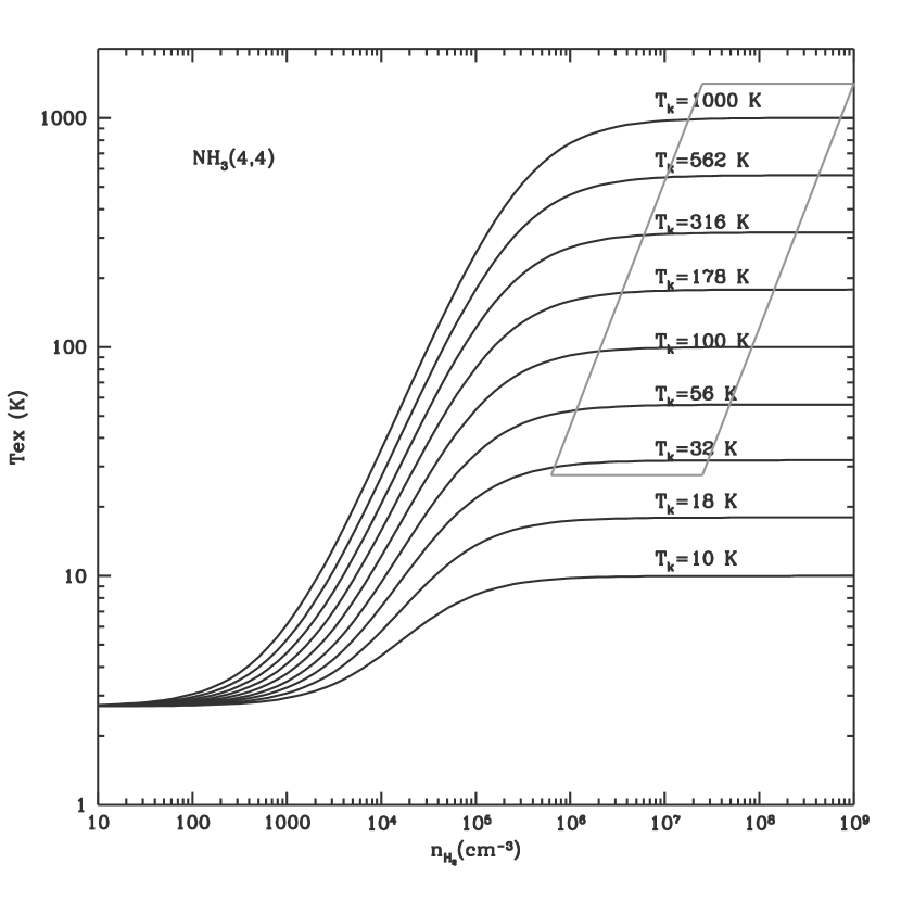
Figure 7: Excitation temperature of the ammonia (4,4) inversion transition as a function of the molecular gas density, for different values of the kinetic temperature, obtained from a two-level model. A local radiation field with the intensity of the cosmological background field, at 2.7 K, has been assumed. For emission lines, this gives a lower limit to the excitation temperature. Note that the transition is well thermalized, $T_{\rm ex}\simeq T_{k}$, for the range of densities and kinetic temperatures of HMCs, which is indicated by a box.

As an example, Figure 7 shows the excitation temperature for the ammonia (4,4) inversion transition as a function of the density for a range of kinetic temperatures from 10 to 1000 K. As can be seen from the figure, the transition is well thermalized for the density and temperature ranges of HMCs. A similar result is obtained for transitions (1,1) to (5,5).

Appendix B Calculation of the Absorption Coefficient of the NH₃ Inversion Transitions

The absorption coefficient corresponding to a transition between two levels is given by (Estalella & Anglada 1999):

$$\kappa(V)={c^{3}\over 8\pi\nu_{0}^{3}}A_{ul}n_{u}\left(e^{h\nu_{0}/{kT_{\rm ex}}}-1\right)\phi(V),$$ (B1)

where $n_{u}$ is the number density of particles in the upper level, and $\phi(V)$ is the profile function that contains the dependence on the line-of sight velocity. The profile function is actually the line-of-sight velocity distribution function, and is normalized so that $\int_{-\infty}^{+\infty}\phi(V)dV=1$.

For the inversion transition of the $(J,K)$ rotational level of the ammonia molecule, the absorption coefficient is given by

$$\kappa(V)={c^{3}\over 8\pi\nu_{0}^{3}}A_{ul}n_{u}\left(e^{h\nu_{0}/{kT_{\rm ex}}}-1\right)\sum_{i=1}^{5}x_{i}\phi_{i}(V),$$ (B2)

where $\nu_{0}$ is the rest frequency of the main line ($i=3$) of the inversion transition (the values adopted are listed in Table 4 for metastable levels up to $J=6$), $A_{ul}$ is obtained from equation (A3) and listed in Table 4, $n_{u}$ is the number density of ammonia molecules in the upper level of the $(J,K)$ inversion doublet, and $T_{\rm ex}$ is the excitation temperature that describes the relative populations of the inversion doublet and is calculated using equation (A1). Due to the quadrupole hyperfine structure of the ammonia inversion doublet, the profile function is given by $\phi(V)=\sum_{i=1}^{5}x_{i}\phi_{i}(V)$, where $x_{i}$ is the LTE relative intensity of the ith hyperfine component given in Table 5, and $\phi_{i}(V)$ its profile function that is assumed to be a Gaussian. Since the profile function of the overall inversion transition is normalized, $\int_{-\infty}^{+\infty}\sum_{i=1}^{5}x_{i}\phi_{i}(V)dV=1$, and because $\sum_{i=1}^{5}x_{i}=1$, the profile function of each individual hyperfine component should be also normalized, so that, $\int_{-\infty}^{+\infty}\phi_{i}(V)dV=1$. Therefore,

$$\phi_{i}(V)={1\overwithdelims( )2\pi}^{1/2}{1\over\sigma_{V}}e^{-(V-V_{i}-V_{c}-V_{s})^{2}/2\sigma_{V}^{2}},$$ (B3)

where $V_{i}$ is the Doppler velocity corresponding to the frequency shift of each hyperfine component with respect to the main line ($V_{3}=0$), $V_{c}$ is the line-of-sight LSR velocity of the ambient cloud, $V_{s}$ is the line-of-sight component of the systematic velocity field, and $\sigma_{V}$ is the local dispersion of the distribution of line-of-sight velocities due to turbulent and thermal motions.

The density of molecules in the upper level of the inversion doublet, that is required in equation (B2), can be written in terms of the density of molecules in the $(J,K)$ rotational state, $n_{JK}=n_{u}+n_{l}$, using the Boltzmann equation and the excitation temperature,

$$n_{u}={n_{JK}\over 1+e^{h\nu_{0}/kT_{\rm ex}}}.$$ (B4)

On the other hand, the total density of ammonia molecules is given by the sum of the densities of all the rotational states,

$$n_{\rm NH_{3}}=\sum^{\infty}_{J^{\prime}=0}\sum^{J^{\prime}}_{K^{\prime}=0}n_{J^{\prime}K^{\prime}}.$$ (B5)

Using the Boltzmann equation, the density of ammonia molecules in the rotational state $(J,K)$ can be related to the density in any other rotational state $(J^{\prime},K^{\prime})$ through

$${n_{J^{\prime}K^{\prime}}\over n_{JK}}={g_{J^{\prime}K^{\prime}}\over g_{JK}}e^{-(E_{J^{\prime}K^{\prime}}-E_{JK})/kT_{JK,J^{\prime}K^{\prime}}},$$ (B6)

where $g_{JK}$ and $g_{J^{\prime}K^{\prime}}$ are the statistical weights of the two rotational states, $E_{\rm JK}$ and $E_{J^{\prime}K^{\prime}}$ their rotational energies, and $T_{JK,J^{\prime}K^{\prime}}$ is the corresponding rotational temperature. The statistical weights are given by the relations

$$g_{JK}=\left\{\begin{array}[]{ll}4(2J+1),&K\neq\dot{3}\\ 8(2J+1),&K=\dot{3},\ K\neq 0\\ 4(2J+1),&K=0,\end{array}\right.$$ (B7)

and the rotational energies are given by

$$E_{JK}=h[BJ(J+1)+(C-B)K^{2}]~{}~{}~{}(J=0,1,2,\dots;K=0,\pm 1,\ldots,\pm J),$$ (B8)

where $B=2.98\times 10^{11}$ Hz and $C=1.89\times 10^{11}$ Hz are the rotational constants of the ammonia molecule (Townes & Schawlow 1975).

Solving for $n_{J^{\prime}K^{\prime}}$ in equation (B6) and substituting in equation (B5) one obtains

$$n_{\rm NH_{3}}={n_{JK}\over g_{JK}}\sum^{\infty}_{J^{\prime}=0}\sum^{J^{\prime}}_{K^{\prime}=0}g_{J^{\prime}K^{\prime}}e^{-(E_{J^{\prime}K^{\prime}}-E_{JK})/kT_{JK,J^{\prime}K^{\prime}}}.$$ (B9)

Solving the above equation for $n_{JK}$ and substituting the result in equation (B4), the population of molecules in the upper level of the inversion doublet $n_{u}$ can be obtained in terms of $n_{\rm NH_{3}}$,

$$n_{u}={n_{\rm NH_{3}}g_{JK}\over(1+e^{h\nu_{0}/kT_{\rm ex}})\sum^{\infty}_{J^{\prime}=0}\sum^{J^{\prime}}_{K^{\prime}=0}g_{J^{\prime}K^{\prime}}e^{-(E_{J^{\prime}K^{\prime}}-E_{JK})/kT_{JK,J^{\prime}K^{\prime}}}}.$$ (B10)

This equation can be finally written in terms of the number density of H₂ molecules, $n_{\rm H_{2}}$, using the fractional ammonia abundance, $X_{\rm NH_{3}}=n_{\rm NH_{3}}/n_{\rm H_{2}}$. Furthermore, if we assume that the relative populations of all the rotational states are characterized by the same rotational temperature, that we call $T_{\rm rot}$ (this is usually the case in high density regions where collisions dominate and all temperatures thermalize to $T_{k}$), the above equation can be written as

$$n_{u}={n_{\rm H_{2}}X_{\rm NH_{3}}g_{JK}e^{-E_{JK}/kT_{\rm rot}}\over(1+e^{h\nu_{0}/kT_{ex}})Q(T_{\rm rot})},$$ (B11)

where $Q(T)$ is the partition function defined as:

$$Q(T)=\sum^{\infty}_{J^{\prime}=0}\sum^{J^{\prime}}_{K^{\prime}=0}g_{J^{\prime}K^{\prime}}e^{-E_{J^{\prime}K^{\prime}}/kT}.$$ (B12)

In the calculation of $Q(T)$ usually only metastable rotational states ($J=K$) need to be included, since non-metastable states are short lived and in general are not significantly populated. The sum is extended up to a value of $J^{\prime}$ high enough so that the contribution of higher levels is negligible.

Substituting equations (B11) and (B3) into (B2), the expression for the absorption coefficient for the inversion transition of the $(J,K)$ rotational state of the ammonia molecule becomes

$$\kappa(V) = {\left(1\over 128\pi^{3}\right)^{1/2}{c^{3}A_{ul}\over\nu_{0}^{3}}{n_{\rm H_{2}}X_{\rm NH_{3}}\over\sigma_{V}}{e^{h\nu_{0}/kT_{\rm ex}}-1\over e^{h\nu_{0}/kT_{\rm ex}}+1}}$$ (B13)

$$\times{g_{JK}e^{-E_{JK}/kT_{\rm rot}}\over Q(T_{\rm rot})}\sum_{i=1}^{5}x_{i}e^{-(V-V_{i}-V_{c}-V_{s})^{2}/2\sigma_{V}^{2}}.$$

Appendix C Condensation and Sublimation of Molecular Species

Let’s assume a molecular species whose total amount remains constant, while the solid versus gas phase ratio, $\eta$, changes as a result of condensation and sublimation processes due to variations in temperature and density. Let’s further assume that there is a small residual fraction of molecules that remain in the gas phase even at temperatures well below the characteristic sublimation temperature, as observations suggest that the abundance of some molecular species does not drop to zero in the very low temperature regions. Let’s call $X_{\rm min}$ the minimum gas-phase molecular abundance, reached at low temperatures (where $\eta\gg 1$), and $X_{\rm max}$ the maximum gas-phase abundance, reached in the hot regions ($\eta=0$), where all the molecules are in the gas phase. Therefore, $X_{\rm mol}$, the gas-phase molecular abundance at a given point will fulfill the following equation:

$$X_{\rm mol}+\eta(X_{\rm mol}-X_{\rm min})=X_{\rm max},$$ (C1)

where the first term corresponds to the fraction of molecules in the gas-phase and the second term corresponds to the fraction in the solid phase, after correcting for the residual fraction of molecules (corresponding to $X_{\rm min}$) that do not follow the condensation/sublimation process.

Therefore, the gas-phase molecular abundance can be estimated as

$$X_{\rm mol}={{X_{\rm max}-X_{\rm min}}\over{1+\eta}}+X_{\rm min}.$$ (C2)

Following Sandford & Allamandola (1993), the ratio, $\eta$, of molecules in the solid to gas phase, assuming that only thermal processes are involved, can be obtained as

$$\eta=\left({2\pi n_{g}a_{\rm g}^{2}\over\nu_{v}}\right)\left({kT_{k}\over m_{\rm mol}}\right)^{1/2}\exp(E/kT_{k})$$ (C3)

where $n_{g}$ is the number density of dust grains, $a_{g}$ is the grain radius, $\nu_{v}$ is the lattice vibrational frequency of the molecule, $m_{\rm mol}$ is the mass of the molecule, and $E$ is the binding energy of the molecule on the ice surface. For the physical conditions of HMCs the exponential term, defined by the binding energy $E$, dominates the behavior of this equation. Assuming a given dust-to-gas mass ratio, $R$, the density of dust grains can be written in terms of the density, $n$, of gas molecules as $n_{g}=3\mu_{m}m_{\rm H}Rn/(4\pi a_{g}^{3}\rho_{g})$, where $\mu_{m}$ is the mean molecular weight, $m_{\rm H}$ is the mass of the H atom, and $\rho_{g}$ is the density of the material constituting the dust grains. Assuming an average radius of the grains $a_{g}\simeq 0.1$ $\mu$m (see $\S$ 2.3), a ratio $R=1/100$, and a density $\rho_{g}\simeq$ 3 g cm^-3 (Draine & Lee 1984), we obtain $n_{g}\simeq 3\times 10^{-12}n$ and equation (C3) can be written in terms of the gas density.

For the case of sublimation of ammonia ices, substitution of the values of $\nu_{v}=3.45\times 10^{12}$ Hz and $E/k=3075$ K (Sandford & Allamandola 1993) into equation (C3) gives

$$\eta_{\rm NH_{3}}=5\times 10^{-30}\left({n_{\rm H_{2}}\over{\rm cm^{-3}}}\right)\left({T_{k}\over{\rm K}}\right)^{1/2}\exp({\rm 3075~{}K}/T_{k}).$$ (C4)

In the case that the ammonia molecules are trapped into water ice, we substitute the corresponding numerical constants for water, namely $\nu_{\rm v}=2\times 10^{12}$ Hz and $E/k=5070$ K (Sandford & Allamandola 1993) into equation (C3), and the equation becomes

$$\eta_{\rm H_{2}O}=8\times 10^{-30}\left({n_{\rm H_{2}}\over{\rm cm^{-3}}}\right)\left({T_{k}\over{\rm K}}\right)^{1/2}\exp({\rm 5070~{}K}/T_{k}).$$ (C5)

Table 1: Compilation of the Observational Dust Data of G31 HMC

		Angular	Flux	Aperture
$\lambda$		Resolution	Density	Size
($\mu$m)	Instrument	(′′)	(Jy)	(′′)	Refs.
12	MSX	18	$2.0\pm 0.1$	$\sim$ 18	1
12	IRAS	30	$4.1\pm 0.3$	$\sim$ 30	2
21	MSX	18	$15.0\pm 0.9$	$\sim$ 18	1
25	IRAS	30	$52\pm 4$	$\sim$ 30	2
60	IRAS	60	$1090\pm 170$	$\sim$ 60	2
100	IRAS	120	$2820\pm 400$	$\sim$ 120	2
450	SCUBA	9	$227\pm 56$	$\sim$ 150	3
850	SCUBA	15	$55\pm 3$	$\sim$ 150	3
880	SMA	0.8	$21\pm 4$	$\sim$ 8	4
1300	OVRO	3.6	$4.0\pm 0.8$	$\sim$ 7	5
1300	3m IRTF	90	$14.2\pm 0.5$	$\sim$ 90	6
1350	SCUBA	22	$4.9\pm 1.0$	$\sim$ 22	3
1400	PdBI	0.7	$4.4\pm 0.9$	$\sim$ 10	7
1400	BIMA	0.5	$3.6\pm 0.7$	$\sim$ 3	8
2000	SCUBA	34	$2.9\pm 0.6$	$\sim$ 34	3
2700	PdBI	2.1	$0.7\pm 0.2$	$\sim$ 5	9
3300	PdBI	1.8	$0.6\pm 0.2$	$\sim$ 10	7
3400	OVRO	4.7	$0.28\pm 0.18$	$\sim$ 10	5
7000	VLA	0.05	$0.0034\pm 0.0005$	$\cdots$	10
13000	VLA	2.2	$0.05\pm 0.01$	$\sim$ 5	11

References. — (1) Crowther & Conti 2003; (2) IRAS PSC; (3) Hatchell et al. 2000; (4) J.M. Girart, priv. comm.; (5) Maxia et al. 2001; (6) Chini et al. 1986; (7) Beltrán et al. 2005; (8) F. Wyrowski, priv. comm.; (9) Cesaroni et al. 1994b; (10) S. Kurtz, priv. comm.; (11) Cesaroni et al. 1994a.

Table 2: Parameters Derived from the SED Fitting of G31 HMC

	$M_{*}$	${\dot{M}}$	$\beta$	$R_{\rm dust}$	$L_{*}$	$L_{\rm acc}$	$T_{\rm 1000}$	$n_{\rm 1000}$	$V_{\rm 1000}$	$\sigma_{\rm 1000}$	$M_{\rm env}$	$t$	$r_{\rm ew}$	$P_{0}$	$B$
Model	($M_{\odot}$)	($M_{\odot}$ yr-1)		(AU)	($L_{\odot}$)	($L_{\odot}$)	(K)	(cm-3)	(km s-1)	(km s-1)	($M_{\odot}$)	(yr)	(AU)	(dyn cm-2)	(mG)
I	25	$2.6\times 10^{-3}$	1.0	156	$79000$	$1.5\times 10^{5}$	342	$3.1\times 10^{7}$	4.9	0.78	$1.5\times 10^{3}$	$3.9\times 10^{4}$	$2.3\times 10^{4}$	$2.2\times 10^{-6}$	5.2
II	15	$2.3\times 10^{-3}$	1.0	115	$21000$	$7.5\times 10^{4}$	296	$4.2\times 10^{7}$	3.2	0.91	$2.1\times 10^{3}$	$2.7\times 10^{4}$	$1.5\times 10^{4}$	$4.0\times 10^{-6}$	7.1
III	12	$2.0\times 10^{-3}$	1.0	97	$10300$	$5.3\times 10^{4}$	263	$4.4\times 10^{7}$	2.7	0.95	$2.2\times 10^{3}$	$2.4\times 10^{4}$	$1.3\times 10^{4}$	$4.6\times 10^{-6}$	7.6
IV	9	$1.8\times 10^{-3}$	1.0	82	$4000$	3$.6\times 10^{4}$	234	$4.9\times 10^{7}$	2.1	1.03	$2.6\times 10^{3}$	$2.0\times 10^{4}$	$1.1\times 10^{4}$	$6.1\times 10^{-6}$	8.7
V	7	$1.6\times 10^{-3}$	1.0	70	$1800$	$2.5\times 10^{4}$	212	$5.7\times 10^{7}$	1.7	1.05	$2.8\times 10^{3}$	$1.7\times 10^{4}$	$8.8\times 10^{3}$	$7.4\times 10^{-6}$	9.7
VI	5	$1.5\times 10^{-3}$	1.0	62	550	$1.7\times 10^{4}$	194	$7.3\times 10^{7}$	1.1	1.20	$3.6\times 10^{3}$	$1.3\times 10^{4}$	$6.6\times 10^{3}$	$1.22\times 10^{-5}$	12.4
VII	4	$1.4\times 10^{-3}$	1.0	54	240	$1.2\times 10^{4}$	180	$8.3\times 10^{7}$	0.9	1.22	$3.9\times 10^{3}$	$1.2\times 10^{4}$	$5.7\times 10^{3}$	$1.42\times 10^{-5}$	13.4
VIII	3	$1.2\times 10^{-3}$	1.0	46	80	$7.9\times 10^{3}$	163	$9.6\times 10^{7}$	0.7	1.28	$4.4\times 10^{3}$	$1.0\times 10^{4}$	$4.6\times 10^{3}$	$1.81\times 10^{-5}$	15.2
IX	2	$1.2\times 10^{-3}$	1.1	43	16	$5.2\times 10^{3}$	160	$1.5\times 10^{8}$	0.3	1.51	$6.6\times 10^{3}$	$6.7\times 10^{3}$	$3.1\times 10^{3}$	$3.97\times 10^{-5}$	22.4
X	1.5	$1.1\times 10^{-3}$	1.1	37	5	$3.5\times 10^{3}$	145	$1.8\times 10^{8}$	0.2	1.60	$7.7\times 10^{3}$	$5.6\times 10^{3}$	$2.5\times 10^{3}$	$5.40\times 10^{-5}$	26.1
XI	1	$1.0\times 10^{-3}$	1.2	33	0.7	$2.2\times 10^{3}$	140	$2.6\times 10^{8}$	0.1	1.84	$1.1\times 10^{4}$	$4.0\times 10^{3}$	$1.7\times 10^{3}$	$1.02\times 10^{-4}$	35.8

Table 3: Parameters of the Best Fit Model of G31 HMC

Parameter	Value
$R_{\rm ext}$	30000 AU
$R_{*}$	$1\times 10^{12}$ cm
$\beta$	1.0
$M_{*}$	20-25 $M_{\odot}$
${\dot{M}}$	2-3 $\times 10^{-3}$ $M_{\odot}$ yr-1
$R_{\rm dust}$	130-160 AU
$L_{*}$	5-8 $\times 10^{4}$ $L_{\odot}$
$L_{\rm acc}$	1.0-1.5 $\times 10^{5}$ $L_{\odot}$
$T(R_{\rm ext})$	40 K
$T(R_{\rm dust})$	1200 K
$r_{\rm 100\,K}$	6000-6500 AU
$M_{\rm env}$	1400-1800 $M_{\odot}$
$t$	3-4 $\times 10^{4}$ yr
$r_{\rm ew}$	1.9-2.3 $\times 10^{4}$ AU
$P_{0}$	2-3 $\times 10^{-6}$ dyn cm-2
$B$	5-6 mG
$X_{\rm min}$	1-4$\times 10^{-8}$
$X_{\rm max}$	2-4$\times 10^{-6}$

Table 4: Parameters of Inversion Transitions of the Ammonia Molecule

	$\nu_{0}$	$A_{ul}$
($J$,$K$)	(GHz)	(s-1)
(1,1)	23.6944955	$1.66838\times 10^{-7}$
(2,2)	23.7226333	$2.23246\times 10^{-7}$
(3,3)	23.8701292	$2.55865\times 10^{-7}$
(4,4)	24.1394163	$2.82264\times 10^{-7}$
(5,5)	24.5329887	$3.08642\times 10^{-7}$
(6,6)	25.0560250	$3.38201\times 10^{-7}$

Table 5: Electric Quadrupole Hyperfine Structure of the NH₃ Molecule

		$\Delta\nu_{i}$	$V_{i}$
$i$	$F_{1}\rightarrow F^{\prime}_{1}$	(MHz)	(km s-1)	$x_{i}$	Notes
(1,1)
1	$0\rightarrow 1$	1.531	$-19.37$	0.11111	external satellite
2	$2\rightarrow 1$	0.613	$-7.75$	0.13889	internal satellite
3	1$\rightarrow$1 + 2$\rightarrow$2	0	0	0.08333+0.41667 = 0.50000	main line
4	$1\rightarrow 2$	$-$0.613	7.75	0.13889	internal satellite
5	$1\rightarrow 0$	$-$1.531	19.37	0.11111	external satellite
(2,2)
1	$1\rightarrow 2$	2.04	$-$25.78	0.05000	external satellite
2	$3\rightarrow 2$	1.31	$-$16.55	0.05185	internal satellite
3	1$\rightarrow$1 + 2$\rightarrow$2 + 3$\rightarrow$3	0	0	0.15000+0.23148+0.41481 = 0.79629	main line
4	$2\rightarrow 3$	$-$1.31	16.55	0.05185	internal satellite
5	$2\rightarrow 1$	$-$2.04	25.78	0.05000	external satellite
(3,3)
1	$2\rightarrow 3$	2.30	$-$28.88	0.02645	external satellite
2	$4\rightarrow 3$	1.71	$-$21.47	0.02678	internal satellite
3	2$\rightarrow$2 + 3$\rightarrow$3 + 4$\rightarrow$4	0	0	0.21164+0.28009+0.40178 = 0.89352	main line
4	$3\rightarrow 4$	$-$1.71	21.47	0.02678	internal satellite
5	$3\rightarrow 2$	$-$2.30	28.88	0.02645	external satellite
(4,4)
1	$3\rightarrow 4$	2.45	$-$30.43	0.01620	external satellite
2	$5\rightarrow 4$	1.95	$-$24.21	0.01629	internal satellite
3	3$\rightarrow$3 + 4$\rightarrow$4 + 5$\rightarrow$5	0	0	0.24305+0.30083+0.39111 = 0.93500	main line
4	$4\rightarrow 5$	$-$1.95	24.21	0.01629	internal satellite
5	$4\rightarrow 3$	$-$2.45	30.43	0.01620	external satellite
(5,5)
1	$4\rightarrow 5$	2.57	$-$31.40	0.01090	external satellite
2	$5\rightarrow 6$	2.12	$-$25.91	0.01094	internal satellite
3	4$\rightarrow$4 + 5$\rightarrow$5 + 6$\rightarrow$6	0	0	0.26181+0.31148+0.38299 = 0.95629	main line
4	$6\rightarrow 5$	$-$2.12	25.91	0.01094	internal satellite
5	$5\rightarrow 4$	$-$2.57	31.40	0.01090	external satellite
(6,6)
1	$5\rightarrow 6$	2.63	$-$31.46	0.00783	external satellite
2	$6\rightarrow 7$	2.25	$-$26.92	0.00785	internal satellite
3	5$\rightarrow$5 + 6$\rightarrow$6 + 7$\rightarrow$7	0	0	0.27422+0.31765+0.37677 = 0.96863	main line
4	$7\rightarrow 6$	$-$2.25	26.92	0.00785	internal satellite
5	$6\rightarrow 5$	$-$2.63	31.46	0.00783	external satellite

Figure 1: Geometry of the HMC. The plane containing the center of the core and the line of sight is shown. $R_{\rm dust}$ and $R_{\rm ext}$ are the inner and outer radii of the envelope, respectively, $p$ is the impact parameter of the line of sight, $r$ is the radius of a given point, $s$ its coordinate along the line of sight, and $-s_{0}$, $+s_{0}$ are the coordinates of the envelope edges.

Figure 3: Physical structure of the HMC for model I ($M_{*}=25~{}M_{\odot}$; solid line) and models II-XI ($M_{*}$ = 15-1 $M_{\odot}$; dashed lines). (a) Dust temperature as a function of radius; (b) Gas density as a function of radius; (c) Infall velocity as a function of radius; (d) Turbulent velocity dispersion as a function of radius.

Figure 4: Synthetic spectra of the NH${}_{3}(4,4)$ transition (solid line) for model I ($M_{*}=25~{}M_{\odot}$) as a function of the impact parameter, for different values of the gas-phase NH₃ abundance, assumed constant along to the envelope. The values of the abundance are $4\times 10^{-8}$ (left column), $4\times 10^{-7}$ (middle column), and $4\times 10^{-6}$ (right column). The values of the impact parameter are indicated in the upper right corner of each panel. The observed spectra (adapted from Fig. 9c of Cesaroni et al. 1998) are plotted in each panel as dotted lines. The angular resolution is $0\hbox to0.0pt{.\hss}^{\prime\prime}63$.

Figure 5: Synthetic spectra of the NH${}_{3}(4,4)$ transition (solid line) for model I ($M_{*}=25~{}M_{\odot}$) as a function of the impact parameter, assuming a variable gas-phase NH₃ abundance along to the envelope. The values of the minimum, $X_{\rm min}$, and maximum, $X_{\rm max}$, ammonia abundance for each case are given on the top of each column. The best fit model, with $X_{\rm min}=2\times 10^{-8}$ and $X_{\rm max}=3\times 10^{-6}$, is shown in the central column. The values of the impact parameter are indicated in the upper right corner of each panel. The observed spectra (adapted from Fig. 9c of Cesaroni et al. 1998) are plotted in each panel as dotted lines. The angular resolution is $0\hbox to0.0pt{.\hss}^{\prime\prime}63$.

Figure 6: Synthetic spectra (solid line) of the NH${}_{3}(1,1)$, NH${}_{3}(2,2)$, NH${}_{3}(4,4)$, and NH${}_{3}(5,5)$ transitions towards the center of the HMC, for an angular resolution of $40^{\prime\prime}$. The model parameters and the ammonia abundances are the same as in the best model obtained by fitting the high angular resolution NH${}_{3}(4,4)$ data (central column in Fig. 5). The spectra observed with the 100 m telescope (Churchwell et al. 1990, Cesaroni et al. 1992) are also shown (dotted lines). The calibration uncertainty in the observed spectra is 30%.

References

- Ahearn et al. (1986) A’Hearn, M. F., Hoban, S., Birch, P. V., Bowers, C., Martin, R., & Klinglesmith, D. A., III 1986, Nature, 324, 649
- Anglada et al. (1996) Anglada, G., Estalella, R., Pastor, J., Rodriguez, L. F., & Haschick, A. D. 1996, ApJ, 463, 205
- Araya et al. (2003) Araya, E., Hofner, P., Olmi, L., Linz, H., Kurtz, S., & Cesaroni, R. 2003, IAU Symposium, 221, 79P
- Araya et al. (2008) Araya, E., Hofner, P., Kurtz, S., Olmi, L., & Linz, H. 2008, ApJ, 675, 420
- (5) Beltrán, M. T., Cesaroni, R., Neri, R., Codella, C., Furuya, R. S., Testi, L., & Olmi, L. 2005, A&A, 435, 901
- Beuther & Walsh (2008) Beuther, H., & Walsh, A. J. 2008, ApJ, 673, L55
- (7) Boonman, A. M. S., Doty, S. D., van Dishoeck, E. F., Bergin, E. A., Melnick, G. J., Wright, C. M., & Stark, R. 2003, A&A, 406, 937
- Brown et al. (1988) Brown, P. D., Charnley, S. B., & Millar, T. J. 1988, MNRAS, 231, 409
- Cesaroni et al. (1994a) Cesaroni, R., Churchwell, E., Hofner, P., Walmsley, C. M., & Kurtz, S. 1994a, A&A, 288, 903
- Cesaroni et al. (1998) Cesaroni, R., Hofner, P., Walmsley, C. M., & Churchwell, E. 1998, A&A, 331, 709
- Cesaroni et al. (1994b) Cesaroni, R., Olmi, L., Walmsley, C. M., Churchwell, E., & Hofner, P. 1994b, ApJ, 435, L137
- Cesaroni, Walmsley, & Churchwell (1992) Cesaroni, R., Walmsley, C. M., & Churchwell, E. 1992, A&A, 256, 618
- Chini et al. (1986) Chini, R., Kreysa, E., Mezger, P. G., & Gemuend, H.-P. 1986, A&A, 154, L8
- (14) Churchwell, E., Walmsley, C. M., & Cesaroni, R. 1990, A&AS, 83, 119
- Cohen & Poynter (1974) Cohen, E. A., & Poynter, R. L. 1974, Journal of Molecular Spectroscopy, 53, 131
- D’Alessio (1996) D’Alessio, P. 1996, PhD Thesis, Universidad Nacional Autónoma de México
- (17) Danby, G., Flower, D. R., Valiron, P., Schilke, P., & Walmsley, C. M. 1988, MNRAS, 235, 229
- (18) De Buizer, J. M., Osorio, M., & Calvet, N. 2005, ApJ, 635, 452
- Doty, van Dishoeck, van der Tak, & Boonman (2002) Doty, S. D., van Dishoeck, E. F., van der Tak, F. F. S., & Boonman, A. M. S. 2002, A&A, 389, 446
- Draine (87) Draine, B. T. 1987, Princeton Observatory Preprint No. 213
- Draine & Lee (1984) Draine, B. T., & Lee, H. M. 1984, ApJ, 285, 89
- (22) Estalella, R., & Anglada, G. 1996, Introducción a la Física del Medio Interestelar (Barcelona: Ediciones Universitat de Barcelona)
- Estalella et al. (1993) Estalella, R., Mauersberger, R., Torrelles, J. M., Anglada, G., Gomez, J. F., Lopez, R., & Muders, D. 1993, ApJ, 419, 698
- (24) Gibb, A. G., Wyrowski, F., & Mundy, L. G. 2004, ApJ, 616, 301
- Hatchell (2000) Hatchell, J., Fuller, G. A., Millar, T. J., Thompson, M. A., & Macdonald, G. H. 2000, A&A, 357, 637
- Herbst (1973) Herbst, E., & Klemperer, W. 1973, ApJ, 185, 505
- Ho (1977) Ho, P. T. P. 1977, PhD Thesis, Massachusetts Institute of Technology
- (28) Ho, P. T. P., & Townes, C. H. 1983, ARA&A, 21, 239
- (29) Hosokawa, T., & Omukai, K. 2008, Massive Star Formation: Observations Confront Theory, ASP Conf. Ser., 387, 255
- Kurtz et al. (1999) Kurtz, S., Cesaroni, R., Churchwell, E., Hofner, P., & Walmsley, C. M. 2000, in Protostars and Planets IV, eds. V. Mannings, A. P. Boss, & S. Russell (Tucson: Univ. of Arizona Press), 299
- (31) Le Bourlot, J., Pineau des Forets, G., Roueff, E., & Schilke, P. 1993, ApJ, 416, L87
- Lizano & Shu (1989) Lizano, S., & Shu, F. H. 1989, ApJ, 342, 834
- Longmore et al. (2007) Longmore, S. N., Burton, M. G., Barnes, P. J., Wong, T., Purcell, C. R., & Ott, J. 2007, MNRAS, 379, 535
- Mathis et al. (1977) Mathis, J. S., Rumpl, W., & Nordsieck, K. H. 1977, ApJ, 217, 425
- Maxia, Testi, Cesaroni, & Walmsley (2001) Maxia, C., Testi, L., Cesaroni, R., & Walmsley, C. M. 2001, A&A, 371, 287
- McLaughlin & Pudritz (1997) McLaughlin, D. E. & Pudritz, R. E. 1997, ApJ, 476, 750
- (37) Millar, T. J. 1997, en IAU Symp. 178, Molecules in Astrophysics: Probes and Processes, ed. E. F. van Dishoeck (Dordrecht: Kluwer), 75
- Ohishi (1997) Ohishi, M. 1997, in IAU Symp. 178, Molecules in Astrophysics: Probes & Processes, ed. E. F. van Dishoeck (Dordrecht: Kluwer), 61
- (39) Olmi, L., Cesaroni, R., Neri, R., & Walmsley, C. M. 1996, A&A, 315, 565
- Osorio (2000) Osorio, M., 2000, PhD Thesis, Universidad Nacional Autónoma de México
- Osorio (1999) Osorio, M., Lizano, S., & D’Alessio, P. 1999, ApJ, 525, 808
- Ossenkopf & Henning (1994) Ossenkopf, V., & Henning, T. 1994, A&A, 291, 943
- Pickett et al. (1998) Pickett, H. M., Poynter, I. R. L., Cohen, E. A., Delitsky, M. L., Pearson, J. C., & Muller, H. S. P. 1998, Journal of Quantitative Spectroscopy and Radiative Transfer, 60, 883
- Sandford & Allamandola (1993) Sandford, S. A. & Allamandola, L. J. 1993, ApJ, 417, 815
- Schaller et al. (1992) Schaller, G., Schaerer, D., Meynet, G., & Maeder, A. 1992, A&AS, 96, 269
- Shu (1977) Shu, F. H. 1977, ApJ, 214, 488
- Sweitzer (1978) Sweitzer, J. S. 1978, ApJ, 225, 116
- Townes & Schawlow (1975) Townes, C.H., Schawlow, A.L. 1975, Microwave Spectroscopy (New York: Dover)
- Ungerechts, Walmsley, & Winnewisser (1980) Ungerechts, H., Walmsley, C. M., & Winnewisser, G. 1980, A&A, 88, 259
- van der Tak, van Dishoeck, Evans, & Blake (2000) van der Tak, F. F. S., van Dishoeck, E. F., Evans, N. J., & Blake, G. A. 2000, ApJ, 537, 283
- Walmsley (1995) Walmsley, C. M. 1995, RevMexAA Serie de Conf., 1, 137
- Walmsley (1997) Walmsley, C. M. 1997, in IAU Symp. 170, CO: Twenty-Five Years of Millimeter-Wave Spectroscopy, eds. W.B. Latter, S.J.E. Radford, P.R. Jevel, J.G. Mangum & J. Bally (Dordrecht: Kluwer), 79
- Walmsley & Ungerechts (1983) Walmsley, C. M., & Ungerechts, H. 1983, A&A, 122, 164
- Warren (1984) Warren, S. G. 1984, Appl. Opt., 23, 1206
- Wilson et al. (2006) Wilson, T. L., Henkel, C., Hüttemeister, S. 2006, A&A, 460, 533