Plasmon oscillations in ellipsoid nanoparticles: beyond dipole approximation

Abstract

The plasmon oscillations of a metallic triaxial ellipsoid nanoparticle have been studied within the framework of the quasistatic approximation. A general method has been proposed for finding the analytical expressions describing the potential and frequencies of the plasmon oscillations of an arbitrary multipolarity order. The analytical expressions have been derived for an electric potential and plasmon oscillation frequencies of the first 24 modes. Other higher orders plasmon modes are investigated numerically.

I Introduction

Quite a number of works were recently devoted to the studies of optical properties of nanodimensional bodies. Special attention has been paid to the metallic nanoparticles, with the help of which one could amplify the near electric field at the frequencies of the localized plasmon resonances ref1 . Possible applications of that effect have been considered. The most developed of them is the use of large local fields near a rough surface for increasing the surface-enhanced Raman scattering (SERS) ref2 . Modification of properties of the radiating atoms by nanobodies of different shape and composition has been the basis for research and development of nanobiosensors ref3 -ref6 , nanolasers ref7 , microscopes that are capable to detect single molecules ref8 , the devices for DNA decoding ref9 , chemical sensors ref10 -ref12 , and many others.

Very recently, the plasmon nanostructures were successfully used in optical devices, in which the diffraction limit had been overcome thus providing an effective interaction between near and far fields, e.g. in hyper- and nanolenses ref13 -ref15 , nanoantennas ref16 -ref20 . Studying optical properties of the plasmon nanoparticles made up a new line of investigation such as “plasmonics” or “nanoplasmonics” ref21 ; ref22 .

The above-mentioned applications are based on properties of single nanoparticles or clusters of such nanoparticles. Today, the optical properties of metallic nanospheres ref23 -ref30 , nanospheroids ref31 -ref34 , and some other nanobodies ref21 ; ref22 ; ref35 , have been sufficiently well studied with the help of known analytical approaches. Many of the other shapes of nanoparticles have been studied only numerically, which is often insufficient for understanding of underlying physics and for development of new nanodevices.

It is astonishing but an important class of nontrivial nanoparticle shapes , which can be described analytically, turns out to be almost uninvestigated. We keep in mind nanoparticles of triaxial ellipsoid shape. Such nanoparticles have very different shapes and are often studied experimentally ref36 -ref39 . Despite a great number of theoretical works ref40 -ref52 devoted to that problem, there had not yet been achieved any appreciable progress in studies of optical properties of triaxial ellipsoids. This is due, first of all, to an extreme mathematical complexity of the problem. In practice, to describe optical properties of triaxial ellipsoid nanoparticles one makes use of a simple solution for a nanoellipsoid in a uniform electric field ref53 that describes only the simplest (“dipole”) plasmon oscillations. Such a description is sufficient if scattering of plane electromagnetic waves by nanoparticle is of interest. But for many nanooptical problems there are no plane waves and such a solution cannot be used. In particular, it does not work when considering an ellipsoidal nanoparticle interaction with highly nonuniform fields, which is fundamentally important for a nanoworld. For example, the radiation fields of atoms, molecules, or quantum dots placed near the nanobodies are essentially not uniform, and they effectively excite not only “dipole”, but more complex plasmon oscillations also. For example, exactly these modes explain very important phenomenon of radiation quenching.

The aim of this work is to study optical properties of a triaxial metallic nanoellipsoid within the quasistatic approximation, in respect to the excitation of high-order plasmon oscillations that are somehow analogous to the quadrupole, octopole, and hexadecapole spherical harmonics. Here we obtain explicit analytical expressions, which is especially important for fast calculations and estimations.

The content of the remaining part of the article is as follows. In section II, general approach to finding the eigen-functions of plasmon oscillation electric field potential and the permittivity (frequencies) corresponding to those oscillations is described. In section III, the above method is applied to determine explicit values of the permittivity and the plasmon mode potentials. In section IV, the graphic illustrations of the found solutions are given and the results obtained are discussed. The geometry of the problem in question is illustrated in Fig.1.

II General method of solution

The localized plasmons naturally arise as the nontrivial solutions of a homogeneous quasistatic problem, that is, the Laplace equations with the corresponding boundary conditions ref54 ; ref55

$$\Delta\phi_{n} = 0,$$

$$\Delta g_{n} = 0,$$

$$\left.\varepsilon_{n}\frac{\partial\phi_{n}}{\partial\mathbf{n}}\right|_{S} = \left.\bar{\varepsilon}\frac{\partial g_{n}}{\partial\mathbf{n}}\right|_{S},$$ (1)

where $\bar{\varepsilon}$ is the permittivity of space around a nanoparticle that we take equal to 1; $\phi_{n}$, $g_{n}$, the plasmon potentials inside and outside a nanoparticle, respectively; $\left.\frac{\partial\phi_{n}}{\partial\mathbf{n}}\right|_{S}$ stands for a normal derivative of the plasmon potential $\phi_{n}$ at a particle surface; $\varepsilon_{n}$, the resonant permittivity corresponding to the plasmon oscillations of the order $n$, and $\Delta$, the Laplace operator. The latter equation in (1) stands for a fulfillment of continuity of the induction normal components . One may show ref54 ; ref55 that a homogeneous system (1) has nontrivial solutions (localized plasmons) for some (negative) parameters $\varepsilon_{n}$ only.  It is naturally to call $\varepsilon_{n}$ as resonant permittivities. If the permittivity of a real particle is close to one of the values $\varepsilon_{n}$ then it will have a plasmon resonance at frequency $\omega_{n}$, at which

$$\varepsilon_{n}\approx\varepsilon\left(\omega_{n}\right).$$ (2)

That frequency $\omega_{n}$ is called the plasmon frequency and can be found if the dispersion law $\varepsilon\left(\omega\right)$ is known. In what follows we will use the Drude’s dispersion law, ${\varepsilon\left(\omega\right)}=1-{\left(\omega_{pl}{/}\omega\right)}^{2}$, where $\omega_{pl}$ is the bulk plasma frequency of nanoparticle material (metal).

The eigenfunctions of the plasmons $\mathbf{e}_{n}\left(\mathbf{r}\right)=-\nabla\phi_{n}\left(\mathbf{r}\right)$ (where $\nabla$ is the gradient operator) are orthogonal in sense that ($n\neq m$)

$$\int\limits_{V}d\mathbf{r}\left(\mathbf{e}_{n}\cdot\mathbf{e}_{m}\right)=0$$ (3)

These eigenfunctions make the complete system, and the solution for a nanoparticle problem in external field $\mathbf{E}^{0}$ may be expanded over  wavefunctions  $\mathbf{e}_{n}\left(\mathbf{r}\right)$ of the  localized plasmons ref55

$$\mathbf{E}\left(\mathbf{r}\right)=\mathbf{E}^{0}\left(\mathbf{r}\right)+\sum\limits_{n}\mathbf{e}_{n}\left(\mathbf{r}\right)\left(\frac{\varepsilon\left(\omega\right)-1}{\varepsilon_{n}-\varepsilon\left(\omega\right)}\right)\frac{\int\limits_{V}d\mathbf{r}\left(\mathbf{e}_{n}\cdot\mathbf{E}^{0}\right)}{\int\limits_{V}d\mathbf{r}\left(\mathbf{e}_{n}\cdot\mathbf{e}_{n}\right)},$$ (4)

where $\varepsilon\left(\omega\right)$ is the dielectric constant of nanoparticle and the integration is performed over a nanoparticle volume. Thus, this problem is reduced to finding the potentials of plasmon modes and corresponding eigenvalues (resonant permittivities).

To determine the properties of localized plasmons in a triaxial nanoellipsoid it is convenient to use an integral formulation, instead of system (1) (see, for instance, ref56 )

$$\phi_{n}\left(\mathbf{r}\right)=\frac{\varepsilon_{n}-1}{4\pi}\int\limits_{V}d\mathbf{r}^{\prime}\left(\left(\nabla^{\prime}\phi_{n}\left(\mathbf{r}^{\prime}\right)\right)\cdot\nabla\right)\frac{{1}}{\left|\mathbf{r}^{\prime}-\mathbf{r}\right|},$$ (5)

where the integration is performed over the nanoparticle volume; $\mathbf{r}^{\prime}$, $\mathbf{r}$ are the coordinates of some two points inside the nanoparticle, and ${\nabla}^{\prime}$, $\nabla$, the operator gradient over the coordinates $\mathbf{r}^{\prime}$, $\mathbf{r}$, respectively. Because the $\mathbf{r}$ point is inside ellipsoid, expression (5) is the integral equation. The solution of (5) gives us both the eigenvalues $\varepsilon_{n}$ and the values of the plasmon potentials at any spatial point inside ellipsoid.

Due to eq.(1),the solution of integral equation (5) is a bounded harmonic function of ellipsoidal symmetry ( ellipsoidal harmonics). The latter may be represented in the form of the Niven’s functions ref57 -ref59 which are the polynomials of the Cartesian coordinates $\left\{x_{1},x_{2},x_{3}\right\}$:

$$\Phi\left(x_{1},x_{2},x_{3}\right) = \left\{\begin{array}[]{cccc}&x_{1}&x_{2}x_{3}&\\ 1&x_{2}&x_{3}x_{1}&x_{1}x_{2}x_{3}\\ &x_{3}&x_{1}x_{2}&\end{array}\right\}$$ (10)

$$\times\Theta_{1}\left(x_{1},x_{2},x_{3}\right)\Theta_{2}\left(x_{1},x_{2},x_{3}\right)...\Theta_{p}\left(x_{1},x_{2},x_{3}\right),$$

where

$$\Theta_{p}\left(x_{1},x_{2},x_{3}\right)=\frac{x_{1}^{2}}{a_{1}^{2}+\theta_{p}}+\frac{x_{2}^{2}}{a_{2}^{2}+\theta_{p}}+\frac{x_{3}^{2}}{a_{3}^{2}+\theta_{p}}-1.$$ (11)

In Eq.(11), $\theta_{p}$ is a constant. By using the ellipsoid coordinates ref57 it is easy to prove that the Niven’s functions (10) are the eigenpotentials of plasmons inside an ellipsoid.

Thus, knowing the eigenfunctions (10) of eqs. (1) and (5) one can represent the corresponding eigenvalues ( resonant values of permittivity)  in the following form

$$\varepsilon_{n}=1+\left\{\frac{1}{4\pi\phi_{n}\left(\mathbf{r}\right)}\int\limits_{V}d\mathbf{r}^{\prime}\left(\left(\nabla^{\prime}\phi_{n}\left(\mathbf{r}^{\prime}\right)\right)\cdot\nabla\right)\frac{1}{\left|\mathbf{r}^{\prime}-\mathbf{r}\right|}\right\}^{-1},$$ (12)

and the problem is thereby reduced to calculating the integral of the Niven’s functions (10) over a nanoellipsoid volume. The integration can be made by using the Dyson’s theorem ref60 ; ref61 (see Appendix A). According to it, an integral over an ellipsoid volume of a polynomial times Green function $1/\left|\mathbf{r}^{\prime}-\mathbf{r}\right|$, proves to be the polynomial as well, whose power is greater by two

$$\int\limits_{V}d\mathbf{r}^{\prime}\frac{x_{1}^{\prime}{}^{p}x_{2}^{\prime}{}^{q}x_{3}^{\prime}{}^{s}}{\left|\mathbf{r}^{\prime}-\mathbf{r}\right|}=P_{p+q+s+2}\left(x_{1},x_{2},x_{3}\right),$$ (13)

where $P_{p+q+s+2}\left(x_{1},x_{2},x_{3}\right)$ is the polynomial of the Cartesian coordinates ($\sum\limits_{\alpha=1}^{3}\left(x_{\alpha}/a_{\alpha}\right)^{2}<1$) of the power $p+q+s+2$.

To find a solution for the plasmonic oscillation potential outside an ellipsoid one can use again (5)

$$g_{n}\left(r\right)=\frac{\varepsilon_{n}-1}{4\pi}\int\limits_{V}d\mathbf{r}^{\prime}\left(\left(\nabla^{\prime}\phi_{n}\left(\mathbf{r}^{\prime}\right)\right)\cdot\nabla\right)\frac{1}{\left|\mathbf{r}^{\prime}-\mathbf{r}\right|}.$$ (14)

but in eq.(14), unlike (5), $\mathbf{r}$ are coordinates of the point outside the ellipsoid. Knowing the electric potential of plasmon oscillations inside and outside a nanoellipsoid, as well as the corresponding values of the permittivity $\varepsilon_{n}$, one can find electric fields near and inside ellipsoidal nanoparticles in an arbitrary external field (4).

III Functions of electric potential and values of permittivity corresponding to plasmon oscillations of a triaxial nanoellipsoid

In this section, we will apply our general method  to find the plasmonic modes of the power $n=1,2,3,4$.

The case $n=1$ “dipole” modes

Here, in accordance with (10), the potential inside the ellipsoid is linear over the coordinates

$$\phi_{1}=\sum\limits_{\alpha=1}^{3}A_{1}^{\left(\alpha\right)}x_{\alpha}.$$ (15)

By substituting (15) into (5), and making the required differentiation and integration by the Dyson’s theorem (see Appendix A) we obtain the following system of equations:

$$A_{1}^{\left(\alpha\right)}=-\frac{1}{2}\left(\varepsilon_{1}-1\right)a_{1}a_{2}a_{3}I_{\alpha}A_{1}^{\left(\alpha\right)},$$ (16)

where $I_{\alpha}=\int\limits_{0}^{\infty}\frac{du}{\left(u+a_{\alpha}^{2}\right)R\left(u\right)}$ and $R\left(u\right)=\prod\limits_{\alpha=1}^{3}\sqrt{u+a_{\alpha}^{2}}$. As follows from (16), there are three different eigen-functions ($\alpha=1,2,3$) describing the electric potential of the plasmonic oscillations

$$\phi_{1}^{\left(\alpha\right)}=x_{\alpha},$$ (17)

and three  corresponding values of the permittivity

$$\varepsilon_{1}^{\left(\alpha\right)}=1-\left(\frac{a_{1}a_{2}a_{3}}{2}I_{\alpha}\right)^{-1}.$$ (18)

The found eigenfunctions (17) and the eigenvalues (18) are well known and widely used for description of the plasmon resonances in ellipsoid nanoparticles in uniform field ref53 .

The electric potential of the plasmons with $n=1$ outside the particle can be found from (14) by using (17) and (18) (see Appendix B).

The case $n=2$ “quadrupole” modes

Here, the ellipsoid potential is described by the Niven’s functions of two types. Functions of the first type are proportional to $\Theta_{1}\left(x_{1},x_{2},x_{3}\right)$, that is, can be represented in the form:

$$\phi_{2}^{\left({1}\right)}=\sum\limits_{\beta=1}^{3}\frac{x_{\beta}^{2}}{\Lambda^{\prime}-a_{\beta}^{2}}+1,\quad\phi_{2}^{\left({2}\right)}=\sum\limits_{\beta=1}^{3}\frac{x_{\beta}^{2}}{\Lambda^{\prime\prime}-a_{\beta}^{2}}+1,$$ (19)

where ${\Lambda}^{\prime}$ and ${\Lambda}^{\prime\prime}$ are the roots of a quadratic equation $\sum\limits_{\alpha=1}^{3}\frac{1}{\Lambda-a_{\alpha}^{2}}=0$, that is,

$$\left\{\begin{array}[]{c}\Lambda^{\prime}\\ \Lambda^{\prime\prime}\end{array}\right\}=\frac{1}{3}\left\{\pm\left[\sum\limits_{\alpha=1}^{3}\left(a_{\alpha}^{4}-\frac{a_{1}^{2}a_{2}^{2}a_{3}^{2}}{a_{\alpha}^{2}}\right)\right]^{1/2}+\sum\limits_{\alpha=1}^{3}a_{\alpha}^{2}\right\}.$$ (20)

By substituting (19) into (12) and calculating the emerging integrals we obtain explicit expressions for the permittivity of those modes:

$$\varepsilon_{2}^{\left(1\right)} = 1+\left(\frac{a_{1}a_{2}a_{3}}{2}\sum\limits_{\alpha=1}^{3}\frac{a_{\alpha}^{2}I_{\alpha}}{\Lambda^{\prime}-a_{\alpha}^{2}}\right)^{-1},$$

$$\varepsilon_{2}^{\left(2\right)} = 1+\left(\frac{a_{1}a_{2}a_{3}}{2}\sum\limits_{\alpha=1}^{3}\frac{a_{\alpha}^{2}I_{\alpha}}{\Lambda^{\prime\prime}-a_{\alpha}^{2}}\right)^{-1}.$$ (21)

Another type of the solutions for the plasmonic modes with $n=2$ includes three Niven’s functions

$$\phi_{2}^{\left(3\right)}=x_{2}x_{3},\quad\phi_{2}^{\left(4\right)}=x_{3}x_{1},\quad\phi_{2}^{\left(5\right)}=x_{1}x_{2}.$$ (22)

By substituting (22) into (5), and using the Dyson’s theorem one can find the corresponding values of the dielectric permittivity:

$$\varepsilon_{2}^{\left(3\right)} = 1-\left(\frac{a_{1}a_{2}a_{3}}{2}\left(a_{2}^{2}+a_{3}^{2}\right)I_{23}\right)^{-1},$$

$$\varepsilon_{2}^{\left(4\right)} = 1-\left(\frac{a_{1}a_{2}a_{3}}{2}\left(a_{3}^{2}+a_{1}^{2}\right)I_{31}\right)^{-1},$$

$$\varepsilon_{2}^{\left(5\right)} = 1-\left(\frac{a_{1}a_{2}a_{3}}{2}\left(a_{1}^{2}+a_{2}^{2}\right)I_{12}\right)^{-1},$$ (23)

where $I_{\alpha\beta}=\int\limits_{0}^{\infty}\frac{du}{\left(u+a_{\alpha}^{2}\right)\left(u+a_{\beta}^{2}\right)R\left(u\right)}$ ($\alpha,\beta=1,2,3$).

The plasmonic oscillation potentials outside nanoparticle can again be found by using (14) (see Appendix B).

The case $n=3$ “octupole” modes

In this case, the ellipsoid potential is also described by the Niven’s functions of two types. Functions of the first type have the form ($\alpha=1,2,3$)

$$\phi_{3}^{\left(2\alpha-1\right)}=x_{\alpha}\left(\sum\limits_{\gamma=1}^{3}\frac{x_{\gamma}^{2}}{\Lambda_{\alpha}^{\prime}-a_{\gamma}^{2}}+1\right),\quad\phi_{3}^{\left(2\alpha\right)}=x_{\alpha}\left(\sum\limits_{\gamma=1}^{3}\frac{x_{\gamma}^{2}}{\Lambda_{\alpha}^{\prime\prime}-a_{\gamma}^{2}}+1\right).$$ (24)

where $\Lambda_{\alpha}^{\prime}$ and $\Lambda_{\alpha}^{\prime\prime}$ are the roots of the quadratic equation $\sum\limits_{\beta=1}^{3}\frac{1+2\delta_{\alpha\beta}}{\Lambda_{\alpha}-a_{\beta}^{2}}=0$, that is,

$$\left\{\begin{array}[]{c}\Lambda_{\alpha}^{\prime}\\ \Lambda_{\alpha}^{\prime\prime}\end{array}\right\} = \frac{1}{5}\left\{\pm\left[4\sum\limits_{\beta=1}^{3}a_{\beta}^{4}-3a_{\alpha}^{4}-\left(a_{1}a_{2}a_{3}\right)^{2}\left(\sum\limits_{\beta=1}^{3}\frac{1}{a_{\beta}^{2}}+\frac{6}{a_{\alpha}^{2}}\right)\right]^{1/2}\right.$$ (28)

$$\left.+2\sum\limits_{\beta=1}^{3}a_{\beta}^{2}-a_{\alpha}^{2}\right\}.$$

By substituting (24) into (5), and making the required differentiation and integration with the help of the Dyson’s theorem one can find the following expressions for the corresponding resonant dielectric permittivity

$$\varepsilon_{3}^{\left(2\alpha-1\right)} = 1+\left\{\frac{a_{1}a_{2}a_{3}}{4}\left(\Lambda_{\alpha}^{\prime}+2a_{\alpha}^{2}\right)\sum\limits_{\beta=1}^{3}\frac{\left(1+2\delta_{\alpha\beta}\right)a_{\beta}^{2}I_{\alpha\beta}}{\Lambda_{\alpha}^{\prime}-a_{\beta}^{2}}\right\}^{-1},$$

$$\varepsilon_{3}^{\left(2\alpha\right)} = 1+\left\{\frac{a_{1}a_{2}a_{3}}{4}\left(\Lambda_{\alpha}^{\prime\prime}+2a_{\alpha}^{2}\right)\sum\limits_{\beta=1}^{3}\frac{\left(1+2\delta_{\alpha\beta}\right)a_{\beta}^{2}I_{\alpha\beta}}{\Lambda_{\alpha}^{\prime\prime}-a_{\beta}^{2}}\right\}^{-1},$$ (29)

where $\delta_{\alpha\beta}$ is the Kronecker’s delta-symbol equal to unity at $\alpha=\beta$, and equal to zero at $\alpha\neq\beta$.

One more type of the plasmons for $n=3$ is due to only one function of the form

$$\phi_{3}^{\left(7\right)}=x_{1}x_{2}x_{3}.$$ (30)

By substituting (30) into (12), and using the Dyson’s theorem one can find the corresponding values of the permittivity

$$\varepsilon_{3}^{\left(7\right)}=1-\left\{\frac{\left(a_{1}a_{2}a_{3}\right)^{3}}{2}\left(\sum\limits_{\alpha=1}^{3}a_{\alpha}^{-2}\right)I_{123}\right\}^{-1},$$ (31)

where $I_{123}=\int\limits_{0}^{\infty}\frac{du}{R^{3}\left(u\right)}$.

The plasmon electric potentials outside ellipsoid can be found from (14)by using (24)-(31) (see Appendix B).

The case $n=4$ “hexadecapole” modes

Now, there are nine different functions of the plasmon oscillation potentials. Six of them are as follows ($\alpha=1,2,3$)

$$\phi_{4}^{\left(2\alpha-1\right)} = \frac{x_{1}x_{2}x_{3}}{x_{\alpha}}\left(\sum\limits_{\beta=1}^{3}\frac{x_{\beta}^{2}}{\Omega_{\alpha}^{\prime}-a_{\beta}^{2}}+1\right),$$

$$\phi_{4}^{\left(2\alpha\right)} = \frac{x_{1}x_{2}x_{3}}{x_{\alpha}}\left(\sum\limits_{\beta=1}^{3}\frac{x_{\beta}^{2}}{\Omega_{\alpha}^{\prime\prime}-a_{\beta}^{2}}+1\right),$$ (32)

where $\Omega_{\alpha}^{\prime}$ and $\Omega_{\alpha}^{\prime\prime}$ are the roots of equation $\sum\limits_{\beta=1}^{3}\frac{3-2\delta_{\alpha\beta}}{\Omega_{\alpha}-a_{\beta}^{2}}=0$:

$$\left\{\begin{array}[]{c}\Omega_{\alpha}^{\prime}\\ \Omega_{\alpha}^{\prime\prime}\end{array}\right\} = \frac{1}{7}\left(2\sum\limits_{\beta=1}^{3}a_{\beta}^{2}+a_{\alpha}^{2}\right)$$ (36)

$$\pm\frac{1}{7}\left\{4\left(\sum\limits_{\beta=1}^{3}a_{\beta}^{4}-a_{\alpha}^{4}\right)-9a_{\alpha}^{2}\left(\sum\limits_{\beta=1}^{3}a_{\beta}^{2}-2a_{\alpha}^{2}\right)+\frac{a_{1}^{2}a_{2}^{2}a_{3}^{2}}{a_{\alpha}^{2}}\right\}^{1/2}.$$

The rest of the plasmon eigenfunctions are ($\alpha=1,2,3$)

$$\phi_{4}^{\left(6+\alpha\right)}=\left(\sum\limits_{\beta=1}^{3}\frac{x_{\beta}^{2}}{\Xi_{\alpha}^{\prime}-a_{\beta}^{2}}+1\right)\left(\sum\limits_{\beta=1}^{3}\frac{x_{\beta}^{2}}{\Xi_{\alpha}^{\prime\prime}-a_{\beta}^{2}}+1\right),$$ (37)

where $\Xi_{\alpha}^{\prime}$ and $\Xi_{\alpha}^{\prime\prime}$ are three different pairs of the roots of the system of equations:

$$\sum\limits_{\alpha=1}^{3}\frac{1}{\Xi^{\prime}-a_{\alpha}^{2}}+\frac{4}{\Xi^{\prime}-\Xi^{\prime\prime}} = 0,$$

$$\sum\limits_{\alpha=1}^{3}\frac{1}{\Xi^{\prime\prime}-a_{\alpha}^{2}}+\frac{4}{\Xi^{\prime\prime}-\Xi^{\prime}} = 0.$$ (38)

The expressions for $\Xi_{\alpha}^{\prime}$ and $\Xi_{\alpha}^{\prime\prime}$ are rather complicated, so we do not quote them in the explicit form.

The corresponding to (32) values of the permittivity are represented as

$$\varepsilon_{4}^{\left(1\right)} = 1+\frac{4}{a_{1}a_{2}a_{3}}\left\{\left(a_{2}^{2}+a_{3}^{2}\right)^{2}\sum\limits_{\alpha=1}^{3}\frac{\left(1+2\delta_{\alpha 2}+2\delta_{\alpha 3}\right)a_{\alpha}^{2}I_{\alpha 23}}{\Omega_{1}^{\prime}-a_{\alpha}^{2}}\right.$$

$$\left.-\sum\limits_{\alpha=1}^{3}\frac{\left(1+2\delta_{\alpha 2}+2\delta_{\alpha 3}\right)a_{\alpha}^{2}\left(a_{3}^{2}I_{\alpha 2}+a_{2}^{2}I_{\alpha 3}\right)}{\Omega_{1}^{\prime}-a_{\alpha}^{2}}-2\left(a_{2}^{2}+a_{3}^{2}\right)I_{23}\right\}^{-1},$$

$$\varepsilon_{4}^{\left(3\right)} = 1+\frac{4}{a_{1}a_{2}a_{3}}\left\{\left(a_{3}^{2}+a_{1}^{2}\right)^{2}\sum\limits_{\alpha=1}^{3}\frac{\left(1+2\delta_{\alpha 3}+2\delta_{\alpha 1}\right)a_{\alpha}^{2}I_{\alpha 31}}{\Omega_{2}^{\prime}-a_{\alpha}^{2}}\right.$$

$$\left.-\sum\limits_{\alpha=1}^{3}\frac{\left(1+2\delta_{\alpha 3}+2\delta_{\alpha 1}\right)a_{\alpha}^{2}\left(a_{1}^{2}I_{\alpha 3}+a_{3}^{2}I_{\alpha 1}\right)}{\Omega_{2}^{\prime}-a_{\alpha}^{2}}-2\left(a_{3}^{2}+a_{1}^{2}\right)I_{31}\right\}^{-1},$$

$$\varepsilon_{4}^{\left(5\right)} = 1+\frac{4}{a_{1}a_{2}a_{3}}\left\{\left(a_{1}^{2}+a_{2}^{2}\right)^{2}\sum\limits_{\alpha=1}^{3}\frac{\left(1+2\delta_{\alpha 1}+2\delta_{\alpha 2}\right)a_{\alpha}^{2}I_{\alpha 12}}{\Omega_{3}^{\prime}-a_{\alpha}^{2}}\right.$$ (39)

$$\left.-\sum\limits_{\alpha=1}^{3}\frac{\left(1+2\delta_{\alpha 1}+2\delta_{\alpha 2}\right)a_{\alpha}^{2}\left(a_{2}^{2}I_{\alpha 1}+a_{1}^{2}I_{\alpha 2}\right)}{\Omega_{3}^{\prime}-a_{\alpha}^{2}}-2\left(a_{1}^{2}+a_{2}^{2}\right)I_{12}\right\}^{-1},$$

where $I_{\alpha\beta\gamma}=\int\limits_{0}^{\infty}\frac{du}{\left(u+a_{\alpha}^{2}\right)\left(u+a_{\beta}^{2}\right)\left(u+a_{\gamma}^{2}\right)R\left(u\right)}$ ($a,\beta,\gamma=1,2,3$). Expressions for $\varepsilon_{4}^{\left(2\right)}$, $\varepsilon_{4}^{\left(4\right)}$, $\varepsilon_{4}^{\left(6\right)}$ can be obtained via a substitution $\Omega_{\alpha}^{\prime}\rightarrow\Omega_{\alpha}^{\prime\prime}$ from the expressions for $\varepsilon_{4}^{\left(1\right)}$, $\varepsilon_{4}^{\left(3\right)}$, $\varepsilon_{4}^{\left(5\right)}$, respectively.

The remaining three values of the plasmon oscillation permittivity that correspond to functions (37), are of the form ($\alpha=1,2,3)$

$$\varepsilon_{4}^{\left(6+\alpha\right)} = 1+\frac{8}{a_{1}a_{2}a_{3}}\left\{-\sum\limits_{\beta=1}^{3}\sum\limits_{\gamma=1}^{3}\frac{\left(1+2\delta_{\beta\gamma}\right)a_{\beta}^{2}a_{\gamma}^{2}\left(a_{\beta}^{2}+a_{\gamma}^{2}\right)I_{\beta\gamma}}{\left(\Xi_{\alpha}^{\prime}-a_{\beta}^{2}\right)\left(\Xi_{\alpha}^{\prime\prime}-a_{\gamma}^{2}\right)}\right.$$ (40)

$$\left.+\sum\limits_{\beta=1}^{3}\sum\limits_{\gamma=1}^{3}\frac{\left(1-2\delta_{\beta\gamma}\right)a_{\beta}^{2}a_{\gamma}^{2}\left(I_{\beta}+I_{\gamma}\right)}{\left(\Xi_{\alpha}^{\prime}-a_{\beta}^{2}\right)\left(\Xi_{\alpha}^{\prime\prime}-a_{\gamma}^{2}\right)}\right.$$

$$\left.+4\left(\Xi_{\alpha}^{\prime}+\Xi_{\alpha}^{\prime\prime}\right)\sum\limits_{\beta=1}^{3}\frac{a_{\beta}^{2}I_{\beta}}{\left(\Xi_{\alpha}^{\prime}-a_{\beta}^{2}\right)\left(\Xi_{\alpha}^{\prime\prime}-a_{\beta}^{2}\right)}\right\}^{-1}.$$

Expressions for the electric potential outside a nanoellipsoid for $n=4$ can be found from (14) by using (32)-(40).

In the case of the higher-order plasmonic modes ( $n>4)$ the plasmon potentials and the resonant permittivity values of a triaxial nanoellipsoid can be found in analogous way.

To conclude this section, we repeat a general approach to solving a problem of plasmon oscillations in the triaxial nanoellipsoid. First, we find polynomial solutions of the Laplace equation (10) (the Niven’s functions of the respective order). This can always be done. The only problem is to find roots of polynomials of several variables. Then using the Dyson’s theorem we find the integral in Eq.(12) for the eigenvalue. As the integral is known to be proportional to the Niven’s function it is sufficient to find only the highest terms over coordinates, or even one of these terms. The calculation of other terms can be used to check calculations only. Then, by finding the ratio of one the highest terms of Niven’s function to the analogous highest term of the integral we obtain the desired value of the resonant permittivity. Using a dispersion law for a particular substance one can find plasmon frequencies of the modes under consideration.

IV Discussion and analysis of the results obtained

The explicit expressions for plasmon potentials and eigenvalues of the permittivity obtained in the previous section are of great practical importance. From a general solution for a particle in arbitrary external field (4) it is seen that the presence of plasmonic nanoparticles is manifested in two ways. On the one hand, the spatial field distribution near nanoparticles is defined by the eigenfunctions of a corresponding resonant plasmon.So, it is especially important to know spatial properties of the plasmon potentials in the region near nanoparticles (amplification of local fields for SERS and analogous applications), and far from nanoparticles (to couple the near- and far-fields, for the nanoantennas and nanolenses).

The far-field plasmons are characterized by usual multipole moments, so the ALL multipole moments of ALL plasmonic modes should be known. They may be found from expansion of plasmon potentials far from a particle (the mode number is omitted)

$$g\left(r\rightarrow\infty\right)=\frac{1}{r^{3}}\sum\limits_{\alpha=1}^{3}d_{\alpha}x_{\alpha}+\frac{1}{2r^{5}}\sum\limits_{\alpha,\beta=1}^{3}Q_{\alpha\beta}x_{\alpha}x_{\beta}+\frac{1}{6r^{7}}\sum\limits_{\alpha,\beta,\gamma=1}^{3}O_{\alpha\beta\gamma}x_{\alpha}x_{\beta}x_{\gamma}+...$$ (41)

where $\;d_{\alpha},\;Q_{\alpha\beta}$ and $O_{\alpha\beta\gamma}$ are the dipole, quadrupole, and octupole moments, respectively. Multipole moments of different plasmon modes may be found easily by using a operator relation between the interior and exterior Niven’s functions ref57 ; ref59

$$g_{n}=H_{n}\left(\frac{\partial}{\partial x_{1}},\frac{\partial}{\partial x_{2}},\frac{\partial}{\partial x_{3}}\right)\left\{1+\frac{D^{2}}{2\left(2n+3\right)}+\frac{D^{4}}{8\left(2n+3\right)\left(2n+5\right)}+...\right\}\frac{1}{r},$$ (42)

where $H_{n}\left(x_{1},x_{2},x_{3}\right)$ is the polynomial derived from the interior Niven’s functions using the highest coordinate powers only, and where $D^{2}=\sum\limits_{\alpha=1}^{3}a_{\alpha}^{2}\frac{\partial^{2}}{\partial x_{\alpha}^{2}}$ .

At large distance from the origin, every differentiation increases the singularity of $1/r$. The $2^{n}$-th multipole moment of the $n$-th mode will, therefore, be determined by the principal term of Eq.(42)

$$H_{n}\left(\frac{\partial}{\partial x_{1}},\frac{\partial}{\partial x_{2}},\frac{\partial}{\partial x_{3}}\right)\frac{1}{r}=\frac{\left(-1\right)^{n}\left(2n\right)!}{2^{n}n!}\frac{1}{r^{2n+1}}H_{n}\left(x_{1},x_{2},x_{3}\right).$$ (43)

By comparing that expression with the expansion (41) one may find the desired $2^{n}$-th multipole moments of $n$-th mode. The multipole moments of higher powers ($2^{n+1}$, $2^{n+2}$…) can be found from (42) by keeping in series the next terms $D^{2}$, $D^{4}$, …The multipole moments of lower powers ($2^{n-1}$, $2^{n-2}$…) for $n$-th mode will be equal to zero.

On the other hand, the amplitude of plasmon resonance is defined by efficiency of a plasmon excitation. In its turn this efficiency is product of 2 factors. First is the integral of spatial overlapping of external and plasmon field (factor $\int\limits_{V}d\mathbf{r}\left(\mathbf{e}_{n}\cdot\mathbf{E}^{0}\right)$ in Eq.(4)). Second factor is determined by a coincidence of external field frequencies with the resonant plasmon frequency (factor $\left(\varepsilon_{n}-\varepsilon\left(\omega\right)\right)^{-1}$ in (4)). The last one depends considerably on properties of a nanoparticle material. The described features of plasmon resonances in nanoparticles will be analyzed below.

The case $n=1$ “dipole” modes

The electric field of ”dipole” modes inside an ellipsoid nanoparticle is homogeneous (15), and these modes will be most effectively excited by the homogeneous external fields which maximaze overlapping integral $\int\limits_{V}d\mathbf{r}\left(\mathbf{e}_{n}\cdot\mathbf{E}^{0}\right)$. In the case of a highly nonhomogeneous external field, the spacial variations of the field will be averaged and equivalent to a weaker homogeneous field.

A spatial distribution of the squared electric field for modes with $n=1$ is shown in Fig.2 where the ellipsoid axes are $a_{2}/a_{1}=0.6$ and $a_{3}/a_{1}=0.4$. It is seen that for a given geometry there are always two maxima localized at a nanoparticle surface. The mode whose field is along the longest axis has the highest nonhomogeneity (Fig.2, $m=1$). The maximal amplification of the external field by that mode is determined by factor

$$\left|\frac{E}{E^{0}}\right|=\left|\frac{\left(\varepsilon_{1}^{\left(1\right)}-1\right)\varepsilon\left(\omega\right)}{\varepsilon_{1}^{\left(1\right)}-\varepsilon\left(\omega\right)}\right|.$$ (44)

Figure 3 illustrates the surface charge distribution for modes with $n=1$. One can see a quasidipole character of those modes. But unlike the spherical plasmons, the plasmons of ellipsoid nanoparticles have the high-order multipole moments. For the case $n=1$, the quadrupole moment of the mode proves to be zero. For dipole and octupole moments we obtain (see Eq.(41)).

A) For the mode $g_{1}^{\left(1\right)}$ (for more information see Appendix B)

$$d_{\alpha} = -\delta_{\alpha 1}\frac{1}{4\pi}\left(\varepsilon_{1}^{\left(1\right)}-1\right)V,$$

$$O_{\alpha\beta\gamma} = \delta_{\alpha\beta}\delta_{\gamma 1}\frac{9}{20\pi}\left(\varepsilon_{1}^{\left(1\right)}-1\right)\left\{2a_{1}^{2}-5a_{\alpha}^{2}+\sum\limits_{\sigma=1}^{3}a_{\sigma}^{2}\right\}V.$$ (45)

B) For the mode $g_{1}^{\left(2\right)}$

$$d_{\alpha} = -\delta_{\alpha 2}\frac{1}{4\pi}\left(\varepsilon_{1}^{\left(2\right)}-1\right)V,$$

$$O_{\alpha\beta\gamma} = \delta_{\alpha\beta}\delta_{\gamma 2}\frac{9}{20\pi}\left(\varepsilon_{1}^{\left(2\right)}-1\right)\left\{2a_{2}^{2}-5a_{\alpha}^{2}+\sum\limits_{\sigma=1}^{3}a_{\sigma}^{2}\right\}V.$$ (46)

C) For the mode $g_{1}^{\left(3\right)}$

$$d_{\alpha} = -\delta_{\alpha 3}\frac{1}{4\pi}\left(\varepsilon_{1}^{\left(3\right)}-1\right)V,$$

$$O_{\alpha\beta\gamma} = \delta_{\alpha\beta}\delta_{\gamma 3}\frac{9}{20\pi}\left(\varepsilon_{1}^{\left(3\right)}-1\right)\left\{2a_{3}^{2}-5a_{\alpha}^{2}+\sum\limits_{\sigma=1}^{3}a_{\sigma}^{2}\right\}V.$$ (47)

In the case of a sphere ($a_{1}=a_{2}=a_{3}$), the dipole mode has a zero octupole moment, as follows from (45)-(47).

The resonant values of dielectric constant are connected with a corresponding plasmon frequency. Above we found the values of resonance permittivity that are independent of a nanoparticle material. To calculate the plasmon frequencies it is necessary to use the corresponding dispersion laws for real substances. Figure 4 demonstrates the plasmon frequency dependences of the modes with $n=1$ for the Drude’s dispersion law $\omega_{n}=\omega_{pl}{/}\sqrt{1-\varepsilon_{n}}$. It is seen that the plasmon frequencies of all modes have a simple monotonic character. As a whole, the properties of modes with $n=1$ are quite transparent and analogous to dipole modes of a sphere.

The case $n=2$ “qudrupole” modes

Unlike the case with $n=1$, the modes with $n=2$ may be of two types. They are even modes (relative to change of sign of one of the coordinates, two modes) (19) , and odd modes (22) (three modes). Such modes cannot be excited by a homogeneous field of any frequency, because of a overlap integral is equal to zero for such modes. On the other hand, such modes may be excited by fields that are highly nonhomogeneous in the vicinity of a nanoparticle.

A spatial distribution of a squared electric field of the modes with $n=2$ is shown in Fig.5 for an ellipsoid with axes $a_{2}/a_{1}=0.6$ and $a_{3}/a_{1}=0.4$. From this Figure it is seen that for a given geometry there are four maxima and one local minimum of the field. Figure 6 illustrates the surface charge distribution for the same modes. It shows vividly a quasiquadrupole character of these modes.

Below we draw down explicit equations for the dipole, quadrupole, and octopole moments of the modes with $n=2$ (see Eq.(41)). The dipole and octopole moments are zero in this case. For a quadrupole moment we have the following expressions:

A) For the mode $g_{2}^{\left(1\right)}$ (for more information see Appendix B)

$$Q_{\alpha\beta}=-\delta_{\alpha\beta}\frac{3}{5\pi\left(\Lambda^{\prime}-a_{\alpha}^{2}\right)}\left(\varepsilon_{2}^{\left(1\right)}-1\right)\left(\sum\limits_{\gamma=1}^{3}a_{\gamma}^{2}\right)V.$$ (48)

B) For the mode $g_{2}^{\left(2\right)}$

$$Q_{\alpha\beta}=-\delta_{\alpha\beta}\frac{3}{5\pi\left(\Lambda^{\prime\prime}-a_{\alpha}^{2}\right)}\left(\varepsilon_{2}^{\left(2\right)}-1\right)\left(\sum\limits_{\gamma=1}^{3}a_{\gamma}^{2}\right)V.$$ (49)

C) For the mode $g_{2}^{\left(3\right)}$

$$Q_{\alpha\beta}=-\frac{3}{10\pi}\left(\varepsilon_{2}^{\left(3\right)}-1\right)\left(\delta_{\alpha 2}\delta_{\beta 3}a_{2}^{2}+\delta_{\alpha 3}\delta_{\beta 2}a_{3}^{2}\right)V.$$ (50)

D) For the mode $g_{2}^{\left(4\right)}$

$$Q_{\alpha\beta}=-\frac{3}{10\pi}\left(\varepsilon_{2}^{\left(4\right)}-1\right)\left(\delta_{\alpha 1}\delta_{\beta 3}a_{1}^{2}+\delta_{\alpha 3}\delta_{\beta 1}a_{3}^{2}\right)V.$$ (51)

E) For the mode $g_{2}^{\left(5\right)}$

$$Q_{\alpha\beta}=-\frac{3}{10\pi}\left(\varepsilon_{2}^{\left(5\right)}-1\right)\left(\delta_{\alpha 1}\delta_{\beta 2}a_{1}^{2}+\delta_{\alpha 2}\delta_{\beta 1}a_{2}^{2}\right)V.$$ (52)

Figure 7 demonstrates the dependences of plasmon frequencies of the modes with $n=2$ for the Drude’s dispersion law on semi-axis ratio. The plasmon frequencies of the modes with $n=2$ have a nontrivial character with local maxima and minima. In the case of nanoellipsoids of arbitrary shape, the surface $\omega_{2}^{\left(m\right)}\left(a_{3}/a_{1},a_{2}/a_{1}\right)$ has the form of valleys and ridges and has no extremums for nontrivial ellipsoids. From quantum condition that the plasmon frequency is proportional to the plasmon energy it becomes clear, from thermodynamic viewpoint, that nanoparticles with an excited mode are under strain that is minimal at certain geometries. This circumstance could be used in a synthesis of nanoparticles which are optimal for the given plasmons.

From the analysis of Fig.7 it also follows that under certain ratios of $a_{3}/a_{1}$ ($a_{2}/a_{1}$ is fixed), the values of plasmon frequencies corresponding to different indices $m=1,2,\ldots,5$ of the multipolarity $n=2$, may coincide. So, by using a nonhomogeneous source of electromagnetic field one may simultaneously excite several different types (modes) of the plasmon oscillations at one frequency. This fact can be used for development of efficient souces of light and related devicesref50 . When ellipsoid is degenerated into a spheroid ($a_{1}=a_{2}\neq a_{3}$), some of the curves represented in Fig.7 should coincide. In case of multipolarity $n=2$, there should remain only $n+1=3$ independents dispersion curves (and not $2n+1=5$, as for an ellipsoid of general shape). In a particular case of a sphere ($a_{1}=a_{2}=a_{3}$) there will remain only one dispersion point to be determined by the well known expression $\omega=\omega_{pl}\sqrt{2/5}$.

As a whole, the modes with $n=2$, though having much in common with quadrupole modes in a sphere, have a variety of nontrivial properties and may be successfully applied in different nanooptical devices.

The case $n=3$ “octupole” modes

The modes with $n=3$ are described by Eqs. (29) (six modes) and (30) (one mode). They can not be excited by a homogeneous field, because one can show that their dipole moments are equal to zero. However, such modes may be excited by fields which are nonhomogeneous in the vicinity of a particle.

The squared electric field distribution of these modes is shown in Fig.8. It is seen that the field structure is very complex and has several maxima and minima. Note also that the squared field maxima are always on a surface of a nanoparticle.

A surface charge distribution of modes with $n=3$, as shown in Fig.9, is rather complex too. Nevertheless a spatial field structure of those modes can be clearly understood from a simultaneous analysis of Figs. 8 and 9.

Figure 10 illustrates dependences of the plasmon frequencies on one of the ellipsoid semi-axes. These dependences also have the maxima and the minima that can be used in a number of spectroscopic applications.

The case $n=4$ “hexadecapole” modes

Spatial structure of the modes with $n=4$ is more complex, and we do not consider it in this work. We restrict ourselves to dependences of the relative plasmon frequencies $\omega_{4}^{\left(m\right)}/\omega_{pl}$ ($m=1,2,...,9)$ on one of the semi-axes $a_{3}/a_{1}$ ration at the given ratio $a_{2}/a_{1}=0.6$. (Fig.11). These dependences are similar, as a whole, to the lower-order mode dependences, but now one dipsersion curve may have several maxima and minima.

The case $n>4$

As it was mentioned already higher orders plasmonic modes in 3-axial nanoellipsoid can be found analytically within our general approach. Such analytical solution is very complicated and we have restricted our analytical calculations to modes with $n\leq 4$ here.

Nevertheless for the sake of completeness it is important to know (at least qualitatively) properties of all higher modes. To calculate higher orders modes we made use of boundary elements method (BEM, see e.g. ref64 ). This method is based on surface integral equation

$$2\pi\sigma\left(Q\right)=\frac{\varepsilon_{n}-1}{\varepsilon_{n}+1}\int_{S}dS_{M}\sigma\left(M\right)\frac{\left(\mathbf{r}_{MQ}\cdot\mathbf{n}_{Q}\right)}{r_{MQ}^{3}},$$ (53)

which can be derived from volume integral equation (5). Here $\sigma\left(Q\right)$ is surface charge density  of plasmon mode, $\mathbf{n}_{Q}$ is normal to surface of nanoparticles at point $Q$ , $\mathbf{r}_{MQ}$ is radius-vector from point $M$ to point $Q$ and integration is over surface of nanoparticle.Then one can partition surface $S$ of nanoparticle into $N$ small triangle pieces $\Delta S$ and reduce surface integral equation to system of $N$ linear equations.

The results of numerical calculations with 3000 triangles are shown in Fig.12, where dispersion curves of 300 modes are shown by circles while solid lines are analytical dispersion curves from Figures 4, 7 and 10.

From this Figure the general structure of dispersion curves of plasmonic modes in triaxial nanoellipsoid is clearly seen. In the region $a_{3}/a_{1}>0.1$ there is a good agreement between analytical and numerical calculations. On the contrary, in the region $a_{3}/a_{1}<0.1$ numerical solution is inaccurate and  differs substantially from analytical one because of very sharp edges of ellipsoid in this region. The analytical solution show that resonat permittivity goes to infinity or to zero in the limit of very thin ellipsoid $\left(a_{3}/a_{1}\rightarrow 0\right)$.

V Conclusion

In this work, the plasmon oscillations of a triaxial nanoellipsoid have been studied in a quasistatic approximation. A general approach has been proposed to finding analytical expressions for the plasmon electric potentials and the corresponding values of permittivity (or plasmon frequencies) of an arbitrary multipolarity order. By making use of that approach one could derive the explicit analytical expressions for potentials of several plasmon modes and the dielectric permittivity.

The analytical expressions obtained in this work are extremely important for nanoplasmonics and nanooptics. They can be used to interpret the experimental results on optical properties of nanoparticles and to assess reliability of numerical calculations on the interaction of electromagnetic radiation with nanoparticles that may be approximated by triaxial nanoellipsoids.

The variety and complexity of optical properties of the triaxial nanoellipsoids can also be used in many new nanooptical applications. In particular, by choosing a suitable geometry of an ellipsoid one can ensure its effective interaction with elementary quantum emitters both in the radiation and absorption regimes. As a result, the efficiency of natural and artificial fluorophores and other nanodimensional light sources might be substantially enhanced ref50 ; ref62 .

In addition, due to the complexity of geometry of an ellipsoid and its plasmon modes, one might build, on its basis, the effective optical nanoantennas ref15 -ref18 . They possess all properties of more complex in production Yagi-Uda nanoantennas ref63 , and may be more easily synthesized. Of course, a detailed description of a non-dipole radiation pattern of an ellipsoid nanoantenna is possible only beyond the framework of quasistatic approximation only. However, the results obtained in this work make it possible to perform fast estimations. Moreover, within the framework of the longwavelength perturbation theory  one can find next order corrections ($\sim 1/\lambda^{2}$ and $\sim 1/\lambda^{3}$ ) to resonant values of permittivity and the respective eigenfunctions ref62 .

Appendix A The explicit expressions for the integrals used in calculations of the plasmon potentials of a triaxial nanoellipsoid

By F.D. Dyson the following theorem has been proved ref60 ; ref61 ($p,q,s=0,1,2,\ldots$)

$$\int\limits_{V}d\mathbf{r}^{\prime}\frac{x_{1}^{\prime}{}^{p}x_{2}^{\prime}{}^{q}x_{3}^{\prime}{}^{s}}{\left|\mathbf{r}^{\prime}-\mathbf{r}\right|} = \sum\limits_{k=0}^{\left[N/2\right]}\frac{\pi a_{1}a_{2}a_{3}}{2^{2k}k!\left(k+1\right)!}$$ (54)

$$\times\int\limits_{u_{0}}^{\infty}\frac{duu^{k}}{R\left(u\right)}\left(1-\sum\limits_{\alpha=1}^{3}\frac{x_{\alpha}^{2}}{u+a_{\alpha}^{2}}\right)^{k+1}$$

$$\times\hat{D}^{k}\left\{\left(\frac{a_{1}^{2}x_{1}}{u+a_{1}^{2}}\right)^{p}\left(\frac{a_{2}^{2}x_{2}}{u+a_{2}^{2}}\right)^{q}\left(\frac{a_{3}^{2}x_{3}}{u+a_{3}^{2}}\right)^{s}\right\},$$

where $N$=max($p,q,s$); $\hat{D}=\sum\limits_{\alpha=1}^{3}\frac{u+a_{\alpha}^{2}}{a_{\alpha}^{2}}\frac{\partial^{2}}{\partial x_{\alpha}^{2}}$, $\hat{D}^{0}=1$. Basing on this theorem one can obtain analytical expressions for the following integrals used in this work ($\alpha,\beta,\gamma,\sigma=1,2,3$):

$$\int\limits_{V}\frac{d\mathbf{r}^{\prime}}{\left|\mathbf{r}^{\prime}-\mathbf{r}\right|}=\pi a_{1}a_{2}a_{3}\left(I\left(u_{0}\right)-\sum\limits_{\alpha=1}^{3}x_{\alpha}^{2}I_{\alpha}\left(u_{0}\right)\right),$$ (55)

$$\int\limits_{V}d\mathbf{r}^{\prime}\frac{x_{\alpha}^{\prime}}{\left|\mathbf{r}^{\prime}-\mathbf{r}\right|}=\pi a_{1}a_{2}a_{3}a_{\alpha}^{2}x_{\alpha}\left(I_{\alpha}\left(u_{0}\right)-\sum\limits_{\beta=1}^{3}x_{\beta}^{2}I_{\alpha\beta}\left(u_{0}\right)\right),$$ (56)

$$\int\limits_{V}d\mathbf{r}^{\prime}\frac{x_{\alpha}^{\prime}x_{\beta}^{\prime}}{\left|\mathbf{r}^{\prime}-\mathbf{r}\right|} = \pi a_{1}a_{2}a_{3}a_{\alpha}^{2}a_{\beta}^{2}x_{\alpha}x_{\beta}\left(I_{\alpha\beta}\left(u_{0}\right)-\sum\limits_{\gamma=1}^{3}x_{\gamma}^{2}I_{\alpha\beta\gamma}\left(u_{0}\right)\right)$$ (57)

$$+\frac{1}{4}\pi a_{1}a_{2}a_{3}a_{\alpha}^{2}\delta_{\alpha\beta}\left(I\left(u_{0}\right)-2\sum\limits_{\gamma=1}^{3}x_{\gamma}^{2}I_{\gamma}\left(u_{0}\right)\right.$$

$$\left.+\sum\limits_{\gamma=1}^{3}\sum\limits_{\sigma=1}^{3}x_{\gamma}^{2}x_{\sigma}^{2}I_{\gamma\sigma}\left(u_{0}\right)\right)$$

$$-\frac{1}{4}\pi a_{1}a_{2}a_{3}a_{\alpha}^{4}\delta_{\alpha\beta}\left(I_{\alpha}\left(u_{0}\right)-2\sum\limits_{\gamma=1}^{3}x_{\gamma}^{2}I_{\alpha\gamma}\left(u_{0}\right)\right.$$

$$\left.+\sum\limits_{\gamma=1}^{3}\sum\limits_{\sigma=1}^{3}x_{\gamma}^{2}x_{\sigma}^{2}I_{\alpha\gamma\sigma}\left(u_{0}\right)\right),$$

$$\int\limits_{V}d\mathbf{r}^{\prime}\frac{x_{\alpha}^{\prime}x_{\beta}^{\prime}x_{\gamma}^{\prime}}{\left|\mathbf{r}^{\prime}-\mathbf{r}\right|} = \pi a_{1}a_{2}a_{3}a_{\alpha}^{2}a_{\beta}^{2}a_{\gamma}^{2}x_{\alpha}x_{\beta}x_{\gamma}\left(I_{\alpha\beta\gamma}\left(u_{0}\right)-\sum\limits_{\sigma=1}^{3}x_{\sigma}^{2}I_{\alpha\beta\gamma\sigma}\left(u_{0}\right)\right)$$ (58)

$$+\frac{1}{4}\pi a_{1}a_{2}a_{3}\delta_{\alpha\beta}a_{\alpha}^{2}a_{\gamma}^{2}x_{\gamma}\left(I_{\alpha}\left(u_{0}\right)-2\sum\limits_{\sigma=1}^{3}x_{\sigma}^{2}I_{\alpha\sigma}\left(u_{0}\right)\right.$$

$$\left.+\sum\limits_{\sigma=1}^{3}\sum\limits_{\rho=1}^{3}x_{\sigma}^{2}x_{\rho}^{2}I_{\alpha\sigma\rho}\left(u_{0}\right)\right)$$

$$-\frac{1}{4}\pi a_{1}a_{2}a_{3}\delta_{\alpha\beta}a_{\alpha}^{2}a_{\gamma}^{4}x_{\gamma}\left(I_{\alpha\gamma}\left(u_{0}\right)-2\sum\limits_{\sigma=1}^{3}x_{\sigma}^{2}I_{\alpha\gamma\sigma}\left(u_{0}\right)\right.$$

$$\left.+\sum\limits_{\sigma=1}^{3}\sum\limits_{\sigma=1}^{3}x_{\sigma}^{2}x_{\rho}^{2}I_{\alpha\gamma\sigma\rho}\left(u_{0}\right)\right)$$

$$+\frac{1}{2}\pi a_{1}a_{2}a_{3}\delta_{\alpha\beta}\delta_{\alpha\gamma}a_{\alpha}^{4}x_{\alpha}\left(I_{\alpha}\left(u_{0}\right)-2\sum\limits_{\sigma=1}^{3}x_{\sigma}^{2}I_{\alpha\sigma}\left(u_{0}\right)\right.$$

$$\left.+\sum\limits_{\sigma=1}^{3}\sum\limits_{\rho=1}^{3}x_{\sigma}^{2}x_{\rho}^{2}I_{\alpha\sigma\rho}\left(u_{0}\right)\right)$$

$$-\frac{1}{2}\pi a_{1}a_{2}a_{3}\delta_{\alpha\beta}\delta_{\alpha\gamma}a_{\alpha}^{6}x_{\alpha}\left(I_{\alpha\alpha}\left(u_{0}\right)-2\sum\limits_{\sigma=1}^{3}x_{\sigma}^{2}I_{\alpha\alpha\sigma}\left(u_{0}\right)\right.$$

$$\left.+\sum\limits_{\sigma=1}^{3}\sum\limits_{\rho=1}^{3}x_{\sigma}^{2}x_{\rho}^{2}I_{\alpha\alpha\sigma\rho}\left(u_{0}\right)\right),$$

in which $\delta_{\alpha\beta}$ is the Kronecker’s delta-symbol equal to unity at $\alpha=\beta$, and equal to zero at $\alpha\neq\beta$;

$$I\left(u_{0}\right) = \int\limits_{u_{0}}^{\infty}\frac{du}{R\left(u\right)},\quad I_{\alpha}\left(u_{0}\right)=\int\limits_{u_{0}}^{\infty}\frac{du}{\left(u+a_{\alpha}^{2}\right)R\left(u\right)},$$

$$I_{\alpha\beta}\left(u_{0}\right) = \int\limits_{u_{0}}^{\infty}\frac{du}{\left(u+a_{\alpha}^{2}\right)\left(u+a_{\beta}^{2}\right)R\left(u\right)},$$

$$I_{\alpha\beta\gamma}\left(u_{0}\right) = \int\limits_{u_{0}}^{\infty}\frac{du}{\left(u+a_{\alpha}^{2}\right)\left(u+a_{\beta}^{2}\right)\left(u+a_{\gamma}^{2}\right)R\left(u\right)},$$

$$I_{\alpha\beta\gamma\sigma}\left(u_{0}\right) = \int\limits_{u_{0}}^{\infty}\frac{du}{\left(u+a_{\alpha}^{2}\right)\left(u+a_{\beta}^{2}\right)\left(u+a_{\gamma}^{2}\right)\left(u+a_{\sigma}^{2}\right)R\left(u\right)},$$ (59)

where $R\left(u\right)=\prod\limits_{\alpha=1}^{3}\sqrt{u+a_{\alpha}^{2}}$; the parameter $u_{0}=0$, if the point $\mathbf{r}$ is inside an ellipsoid, and $u_{0}$ is the positive root of equation $\sum\limits_{\alpha=1}^{3}\frac{x_{\alpha}^{2}}{u_{0}+a_{\alpha}^{2}}=1$, if point $\mathbf{r}$ is outside the ellipsoid.

Appendix B The explicit expressions for plasmon wavefunction outside ellipsoid (see Eq.(14))

A) In the case $n=1$ we get three functions ($\alpha=1,2,3$)

$$g_{1}^{\left(\alpha\right)}=x_{\alpha}\frac{I_{\alpha}\left(u_{0}\right)}{I_{\alpha}}.$$ (60)

B) In the case $n=2$ we get five functions. Two of them are of the form

$$g_{2}^{\left(1\right)} = \left(\sum\limits_{\beta=1}^{3}\frac{a_{\beta}^{2}I_{\beta}}{\Lambda^{\prime}-a_{\beta}^{2}}\right)^{-1}\left\{\sum\limits_{\beta=1}^{3}\frac{a_{\beta}^{2}I_{\beta}\left(u_{0}\right)}{\Lambda^{\prime}-a_{\beta}^{2}}\left(\sum\limits_{\alpha=1}^{3}\frac{x_{\alpha}^{2}}{\Lambda^{\prime}-a_{\alpha}^{2}}+1\right)\right.$$

$$\left.+\frac{2u_{0}}{R\left(u_{0}\right)}\sum\limits_{\alpha=1}^{3}\frac{x_{\alpha}^{2}}{\left(\Lambda^{\prime}-a_{\alpha}^{2}\right)\left(u_{0}+a_{\alpha}^{2}\right)}\right\},$$

$$g_{2}^{\left(2\right)} = \left(\sum\limits_{\beta=1}^{3}\frac{a_{\beta}^{2}I_{\beta}}{\Lambda^{\prime\prime}-a_{\beta}^{2}}\right)^{-1}\left\{\sum\limits_{\beta=1}^{3}\frac{a_{\beta}^{2}I_{\beta}\left(u_{0}\right)}{\Lambda^{\prime\prime}-a_{\beta}^{2}}\left(\sum\limits_{\alpha=1}^{3}\frac{x_{\alpha}^{2}}{\Lambda^{\prime\prime}-a_{\alpha}^{2}}+1\right)\right.$$ (61)

$$\left.+\frac{2u_{0}}{R\left(u_{0}\right)}\sum\limits_{\alpha=1}^{3}\frac{x_{\alpha}^{2}}{\left(\Lambda^{\prime\prime}-a_{\alpha}^{2}\right)\left(u_{0}+a_{\alpha}^{2}\right)}\right\},$$

where

$$\left\{\begin{array}[]{c}\Lambda^{\prime}\\ \Lambda^{\prime\prime}\end{array}\right\}=\frac{1}{3}\left\{\pm\left[\sum\limits_{\alpha=1}^{3}\left(a_{\alpha}^{4}-\frac{a_{1}^{2}a_{2}^{2}a_{3}^{2}}{a_{\alpha}^{2}}\right)\right]^{1/2}+\sum\limits_{\alpha=1}^{3}a_{\alpha}^{2}\right\}.$$ (62)

The rest three have the form

$$g_{2}^{\left(3\right)}=x_{2}x_{3}\frac{I_{23}\left(u_{0}\right)}{I_{23}},\quad g_{2}^{\left(4\right)}=x_{3}x_{1}\frac{I_{31}\left(u_{0}\right)}{I_{31}},\quad g_{2}^{\left(5\right)}=x_{1}x_{2}\frac{I_{12}\left(u_{0}\right)}{I_{12}}.$$ (63)

C) In the case $n=3$ we get seven functions. Six of them are ($\alpha=1,2,3$)

$$g_{3}^{\left(2\alpha-1\right)} = x_{\alpha}\left(\sum\limits_{\gamma=1}^{3}\frac{\left(1+2\delta_{\alpha\gamma}\right)a_{\gamma}^{2}I_{\alpha\gamma}}{\Lambda_{\alpha}^{\prime}-a_{\gamma}^{2}}\right)^{-1}$$ (64)

$$\times\left\{\sum\limits_{\gamma=1}^{3}\frac{\left(1+2\delta_{\alpha\gamma}\right)a_{\gamma}^{2}I_{\alpha\gamma}\left(u_{0}\right)}{\Lambda_{\alpha}^{\prime}-a_{\gamma}^{2}}\left(\sum\limits_{\beta=1}^{3}\frac{x_{\beta}^{2}}{\Lambda_{\alpha}^{\prime}-a_{\beta}^{2}}+1\right)\right.$$

$$\left.+\frac{2u_{0}}{R\left(u_{0}\right)\left(\Lambda_{\alpha}^{\prime}+2a_{\alpha}^{2}\right)\left(u_{0}+a_{\alpha}^{2}\right)}\left(\sum\limits_{\beta=1}^{3}\frac{\left(2a_{\alpha}^{2}+a_{\beta}^{2}\right)x_{\beta}^{2}}{\left(\Lambda_{\alpha}^{\prime}-a_{\beta}^{2}\right)\left(u_{0}+a_{\beta}^{2}\right)}+1\right)\right\},$$

and

$$g_{3}^{\left(2\alpha\right)} = x_{\alpha}\left(\sum\limits_{\gamma=1}^{3}\frac{\left(1+2\delta_{\alpha\gamma}\right)a_{\gamma}^{2}I_{\alpha\gamma}}{\Lambda_{\alpha}^{\prime\prime}-a_{\gamma}^{2}}\right)^{-1}$$ (65)

$$\times\left\{\sum\limits_{\gamma=1}^{3}\frac{\left(1+2\delta_{\alpha\gamma}\right)a_{\gamma}^{2}I_{\alpha\gamma}\left(u_{0}\right)}{\Lambda_{\alpha}^{\prime\prime}-a_{\gamma}^{2}}\left(\sum\limits_{\beta=1}^{3}\frac{x_{\beta}^{2}}{\Lambda_{\alpha}^{\prime\prime}-a_{\beta}^{2}}+1\right)\right.$$

$$\left.+\frac{2u_{0}}{R\left(u_{0}\right)\left(\Lambda_{\alpha}^{\prime\prime}+2a_{\alpha}^{2}\right)\left(u_{0}+a_{\alpha}^{2}\right)}\left(\sum\limits_{\beta=1}^{3}\frac{\left(2a_{\alpha}^{2}+a_{\beta}^{2}\right)x_{\beta}^{2}}{\left(\Lambda_{\alpha}^{\prime\prime}-a_{\beta}^{2}\right)\left(u_{0}+a_{\beta}^{2}\right)}+1\right)\right\},$$

where

$$\left\{\begin{array}[]{c}\Lambda_{\alpha}^{\prime}\\ \Lambda_{\alpha}^{\prime\prime}\end{array}\right\} = \frac{1}{5}\left\{\pm\left[4\sum\limits_{\beta=1}^{3}a_{\beta}^{4}-3a_{\alpha}^{4}-\left(a_{1}a_{2}a_{3}\right)^{2}\left(\sum\limits_{\beta=1}^{3}\frac{1}{a_{\beta}^{2}}+\frac{6}{a_{\alpha}^{2}}\right)\right]^{1/2}\right.$$ (69)

$$\left.+2\sum\limits_{\beta=1}^{3}a_{\beta}^{2}-a_{\alpha}^{2}\right\}.$$

The rest seventh function is

$$g_{3}^{\left(7\right)}=x_{1}x_{2}x_{3}\frac{I_{123}\left(u_{0}\right)}{I_{123}}.$$ (70)

In the expressions above we have used notations $I_{\alpha}=I_{\alpha}\left(0\right)$, $I_{\alpha\beta}=I_{\alpha\beta}\left(0\right)$ and $I_{\alpha\beta\gamma}=I_{\alpha\beta\gamma}\left(0\right)$ (see Eq. (59)).

It should be noted, if we set $u_{0}=0$ (ellipsoid surface), then the potential functions of an exterior problem, represented in Appendix B, turn into the respective functions of an interior problem.

Fig.1 Geometry of the problem.

Fig.2 (Color online) Distribution of the squared electric field logarithm (a.u.) near a triaxial nanoellipsoid with semi-axes $a_{2}/a_{1}=0.6$ and $a_{3}/a_{1}=0.4$ in the plane $x_{3}=0$ for the plasmon modes with $n=1$. Index $m=1,2,3$ denotes upper index of the potential function $\phi_{1}^{\left(m\right)}$. Transition from red color to blue corresponds to transition from the highest squared values of electric field to the least squared values. Black line corresponds to the surface of the nanoparticle.

Fig.3 (Color online) Surface charge distribution (a.u.) of plasmon modes of a triaxial nanoellipsoid with $n=1$ at $a_{2}/a_{1}=0.6$ and $a_{3}/a_{1}=0.4$. Index $m=1,2,3$ denotes upper index of the potential function $\phi_{1}^{\left(m\right)}$. Warm colors correspond to the positive charge; cold - negative.

Fig.4 (Color online) Relative frequency of plasmon oscillations of a triaxial nanoellipsoid $\omega_{1}^{\left(m\right)}/\omega_{pl}$ as function of semi-axes ratio $a_{3}/a_{1}$ at $a_{2}/a_{1}=0.6$.

Fig.5 (Color online) Distribution of the squared electric field logarithm (a.u.) near a triaxial nanoellipsoid with $a_{2}/a_{1}=0.6$ and $a_{3}/a_{1}=0.4$ with semi-axes $a_{2}/a_{1}=0.6$ and $a_{3}/a_{1}=0.4$ in the plane $x_{3}=0$ for plasmonic modes with $n=2$. Index $m=1,2,\ldots,5$ denotes upper index of the potential function $\phi_{2}^{(m)}$. Transition from red color to blue corresponds to transition from the highest squared values of electric field to the least squared values. Black line corresponds to the surface of the nanoparticle.

Fig.6 (Color online) Surface charge distribution (a.u.) of plasmon modes of a triaxial nanoellipsoid with $n=2$ at $a_{2}/a_{1}=0.6$ and $a_{3}/a_{1}=0.4$. Index $m=1,2,\ldots,5$ denotes upper index of the potential function $\phi_{2}^{(m)}$. Warm colors correspond to the positive charge; cold - negative.

Fig.7 (Color online) Relative frequency of plasmonic oscillations of the triaxial nanoellipsoid $\omega_{2}^{\left(m\right)}/\omega_{pl}$ as the function of semi-axes ratio $a_{3}/a_{1}$ at $a_{2}/a_{1}=0.6$.

Fig.8 (Color online) Distribution of the squared electric field logarithm (a.u.) near a triaxial nanoellipsoid with semi-axes $a_{2}/a_{1}=0.6$ and $a_{3}/a_{1}=0.4$ in the plane $x_{3}=0$ for plasmon modes with $n=3$. Index $m=1,2,\ldots,7$ denotes upper index of the potential function $\phi_{3}^{(m)}$. Transition from red color to blue corresponds to transition from the highest squared values of electric field to the least squared values. Black line corresponds to the surface of the nanoparticle.

Fig.9 (Color online) Surface charge distribution (a.u.) of plasmon modes of a triaxial nanoellipsoid with $n=3$ at $a_{2}/a_{1}=0.6$ and $a_{3}/a_{1}=0.4$. Index $m=1,2,\ldots,7$ denotes upper index of the potential function $\phi_{3}^{(m)}$. Warm colors correspond to the positive charge; cold - negative.

Fig.10 (Color online) Relative frequency of the triaxial nanoellipsoid plasmon oscillations $\omega_{3}^{(m)}/\omega_{pl}$ as function of the semi-axes ratio $a_{3}/a_{1}$ at $a_{2}/a_{1}=0.6$.

Fig.11 (Color online) Relative frequency of the triaxial nanoellipsoid plasmon oscillations $\omega_{4}^{(m)}/\omega_{pl}$ as function of the semi-axes ratio $a_{3}/a_{1}$ at $a_{2}/a_{1}=0.6$.

Fig.12 (Color online) Permittivity of the triaxial nanoellipsoid plasmon oscillations as function of the semi-axes ratio $a_{3}/a_{1}$ at $a_{2}/a_{1}=0.6$. Solid lines represent analytical solution for $n=1$ (blue lines), $n=2$ (green lines) and $n=3$ (red lines). Circles show results of numerical calculations within boundary element method.

Figure 1:

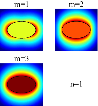
Figure 2:

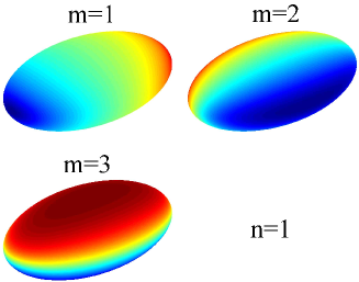
Figure 3:

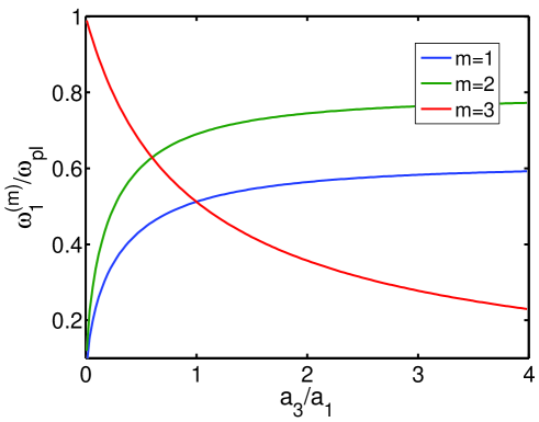
Figure 4:

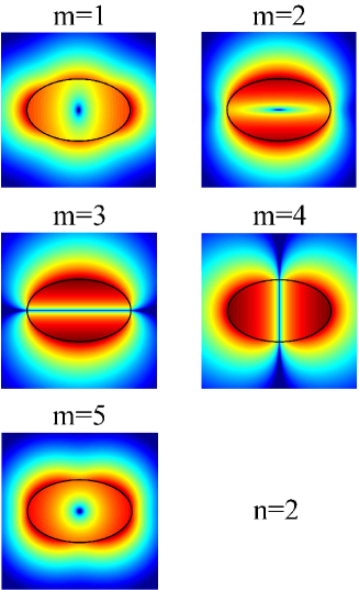
Figure 5:

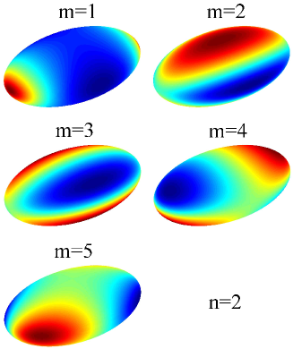
Figure 6:

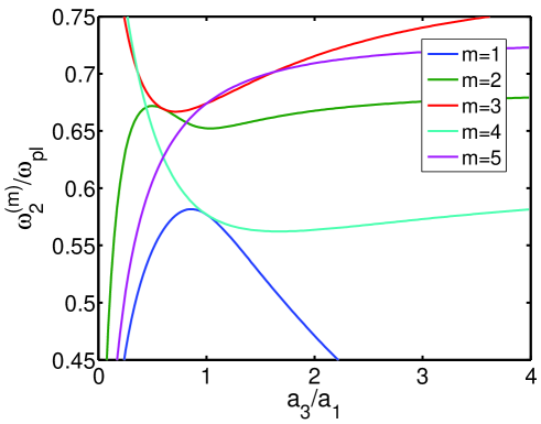
Figure 7:

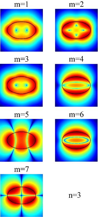
Figure 8:

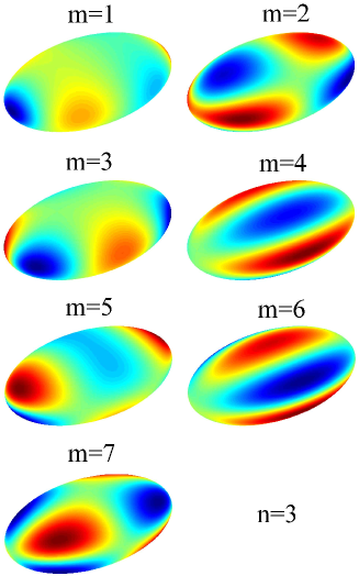
Figure 9:

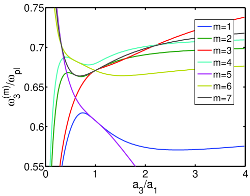
Figure 10:

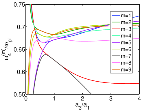
Figure 11:

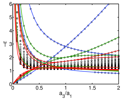
Figure 12:

References

- (1) H. Raether, Surface Plasmons on Rough and Smooth Surfaces and on Gratings (Springer-Verlag, Berlin, 1998).
- (2) Surface-Enhanced Raman Scattering, K. Kneipp, M. Moskovits, H. Kneipp (eds.) (Springer-Verlag, Berlin, 2006).
- (3) Y. Liu, J. Bishop, L. Williams, S. Blair, and J. Herron, Nanotechnology 15, 1368 (2004).
- (4) S. Chah, M.R. Hammond, R.N. Zare, Chemistry & Biology 12, 323 (2005).
- (5) C. Sonnichsen, B.M. Reinhard, J. Liphardt, and A.P. Alivisatos, Nature Biotechnol. 23, 741 (2005).
- (6) M. Brongersma, Nature Materials 2, 296 (2003).
- (7) I.E. Protsenko, A.V. Uskov, O.A. Zaimidoroga, V.N. Samoilov, and E.P. O’Reilly, Phys. Rev. A 71, 063812 (2005).
- (8) V.V. Klimov, M. Ducloy, and V.S. Letokhov, Chem. Phys. Lett. 358, 192 (2002).
- (9) J.R. Lakowicz, J. Malicka, I. Gryczynski, Z. Gryczynski and C.D. Geddes, J. Phys. D: Appl. Phys. 36, R240 (2003).
- (10) K. Kneipp, H. Kneipp, I. Itzkan, R.R. Dasari, M.S. Feld, Chem. Rev. 99, 2957 (1999).
- (11) H.X. Xu, E.J. Bjerneld, M. Kall, L. Borjesson, Phys. Rev. Lett. 83, 4357 (1999).
- (12) T. Vo-Dinh, Trends Anal. Chem. 17, 557 (1998).
- (13) Z. Liu, H. Lee, Y. Xiong, C. Sun and X. Zhang, Science 315, 1686 (2007).
- (14) I.I. Smolyaninov, Y.-J. Hung, and C.C. Davis, Science 315, 1699 (2007).
- (15) S. Kawata, A. Ono and P. Verma, Nature Photonics 2, 438 (2008).
- (16) J. Aizpurua, G.W. Bryant, L.J. Richter, and F.J. García de Abajo, B.K. Kelley and T. Mallouk, Phys. Rev. B 71, 235420 (2005).
- (17) L. Novotny, Phys. Rev. Lett. 98, 266802 (2007).
- (18) P.J. Schuck, D.P. Fromm, A. Sundaramurthy, G.S. Kino, and W.E. Moerner, Phys. Rev. Lett. 94, 017402 (2005).
- (19) P. Muhlschlegel, H.-J. Eisler, O.J.F. Martin, B. Hecht, and D.W. Pohl, Science 308, 1607 (2005).
- (20) O. Muskens, V. Giannini, J. Sanchez-Gil, and J. Gomez-Rivas, Nano Lett. 7, 2871 (2007).
- (21) S.A. Maier, Plasmonics: Fundamentals and Applications (Springer, New York, 2007).
- (22) V.V. Klimov, Nanoplasmonics [in Russian] (Fizmatlit, Moscow, 2008).
- (23) R. Ruppin, J. Chem. Phys. 76, 1681 (1982).
- (24) R. Ruppin, Phys. Rev. B 26, 3440 (1982).
- (25) F. Claro, Phys. Rev. B 25, 7875 (1982).
- (26) M. Danckwerts and L. Novotny, Phys. Rev. Lett. 98, 026104 (2007).
- (27) V.V. Klimov and D.V. Guzatov, Phys. Rev. B 75, 024303 (2007).
- (28) P. Chu and D.L. Mills, Phys. Rev. B 77, 045316 (2008).
- (29) Y.A. Urzhumov, G. Shvets, J. Fan, F. Capasso, D. Brandl, and P. Nordlander, Optics Express 15, 14129 (2007).
- (30) V.V. Klimov, D.V. Guzatov, Appl. Phys. A 89, 305 (2007).
- (31) D.-S. Wang and M. Kerker, Phys. Rev. B 24, 1777 (1981).
- (32) J. Gersten, A. Nitzan, J. Chem. Phys. 75, 1139 (1981).
- (33) V.V. Klimov, M. Ducloy, and V.S. Letokhov, Eur. Phys. J. D 20, 133 (2002).
- (34) A. Trugler and U. Hohenester, Phys. Rev. B 77, 115403 (2008).
- (35) Surface Plasmon Nanophotonics, M.L. Brongersma, P.G. Kik (eds.) (Springer, Dordrecht, 2007).
- (36) C. Sonnichsen, S. Geier, N.E. Hecker, G. Von Plessen, and J. Feldmann, H. Ditlbacher, B. Lamprecht, J.R. Krenn, and F.R. Aussenegg, V.Z-H. Chan, J.P. Spatz, and F.R. Moller, Appl. Phys. Lett. 77, 2949 (2000).
- (37) H.F. Hamann, M. Larbadi, S. Barzen, T. Brown, A. Gallagher, D.J. Nesbitt, Optics Commun. 227, 1 (2003).
- (38) T. Kalkbrenner, U. Hakanson, and V. Sandoghdar, Nano Lett. 4, 2309 (2004).
- (39) J. Grand, P.-M. Adam, A.-S. Grimault, A. Vial, M. Lamy de la Chapelle, J.-L. Bijeon, S. Kostcheev and P. Royer, Plasmonics 1, 135 (2006).
- (40) A.F. Stevenson, J. Appl. Phys. 24, 1143 (1953).
- (41) O.E. Lysenko and N.A. Khizhnyak, Izvestia VUZ. Radiofizika 11, 449 (1968).
- (42) M.L. Levin and R.Z. Muratov, Izvestia VUZ. Radiofizika 22, 512 (1979).
- (43) M. Tejedor, H. Rubio, L. Elbaile, and R. Iglesias, IEEE Trans. Magn. 31, 830 (1995).
- (44) P. Mazeron and S. Muller, Appl. Opt. 35, 3726 (1996).
- (45) G. Perrusson, M. Lambert, D. Lesselier, A. Charalambopoulos, G. Dassios, Radio Science 35, 463 (2000).
- (46) A. Charalambopoulos, G. Dassios, G. Perrusson, D. Lesselier, Int. J. Engineering Science 40, 67 (2002).
- (47) A.A. Oraevsky, A.N. Oraevsky, Quant. Electron. 32, 79 (2002).
- (48) O. Reese and L.C. Lew Yan Voon, M. Willatzen, Phys. Rev. B 70, 075401 (2004).
- (49) A. Irimia, J. Phys. A: Math. Gen. 38, 8123 (2005).
- (50) D.V. Guzatov, V.V. Klimov, Chem. Phys. Lett. 412, 341 (2005).
- (51) A.B. Evlyukhin, S.I. Bozhevolnyi, Surf. Sc. 590, 173 (2005).
- (52) T. Ambjornsson, G. Mukhopadhyay, S.P. Apell and M. Kall, Phys. Rev. B 73, 085412 (2006).
- (53) J.A. Stratton, Electromagnetic Theory (McGraw-Hill, New York, 1941).
- (54) D.J. Bergman and D. Stroud, Solid State Phys. 46, 148 (1992).
- (55) N.N. Voitovich, B.Z. Katsenelenbaum, A.N. Sivov, Generalized method of eigen-oscillations in the theory of diffraction [in Russian] (Nauka, Moscow, 1977).
- (56) W.C. Chew, Waves and fields in inhomogeneous media (IEEE Press, New York, 1995).
- (57) E.W. Hobson, The Theory of Spherical and Ellipsoidal Harmonics (Cambridge University Press, Cambridge, 1931).
- (58) E.T. Whittaker and G.N. Watson, A Course of Modern Analysis (Cambridge University Press, Cambridge, 1963).
- (59) W.D. Niven, Phil. Trans. R. Soc. Lond. A 182, 231 (1891).
- (60) F.D. Dyson, Q. J. Pure Appl. Math. 25, 259 (1891).
- (61) M. Rahman, Proc. R. Soc. Lond. A 457, 2227 (2001).
- (62) D.V. Guzatov and V.V. Klimov, Plasmon oscillations in a triaxial nanoellipsoid: beyond quasistatic approximation (to be published).
- (63) V.V. Klimov and D.V. Guzatov, Optical nanoantennas of triaxial ellipsoid shape (to be published).
- (64) D.R. Fredkin, I.D. Mayergoyz, Phys. Rev. Lett. 91, 253902 (2003).
List of Figure Captions