Benchmarking the solar dynamo with Maxima

Recently, Jouve et al [2] published the paper that presents the numerical benchmark for the solar dynamo models. Here, I would like to show a way how to get it with help of computer algebra system Maxima. This way was used in [4] to test some new ideas in the large-scale stellar dynamos. What you need are the latest version of Maxima-5.16.3 (preferable compiled against the fastest lisps like sbcl or cmucl-sse2) and some knowledge of the global (spectral) methods to solve the PDE eigenvalue problem. For the quite comprehensive introduction to these methods please look at the book by John Boyd [1]. The basic steps to solve the problem are:

1. the mathematical formulation (equation+boundary conditions)

2. choice the basis function and project equations to the basis

3. find matrices (apply some integration procedure in case of Galerkin method)

4. apply linear algebra

The whole consideration is divided for two cases. As the first case we explore the largest free decay modes in the sphere which is submerged in vacuum. In this problem the all dynamo effects are neglected. As the second case I test the $\alpha\Omega$ dynamo in the solar convection zone with the tachocline included.

Lets consider the spherical geometry. The evolution of the axisymmetric large-scale magnetic field (LSMF), $\left\langle\mathbf{B}\right\rangle=\mathbf{e_{\phi}}B+\mathrm{\operatorname{curl}}\left(\frac{A\mathbf{e_{\phi}}}{r\sin\theta}\right)$, (where $r$ is radius, $\theta$- co-latitude, $\mathbf{e}_{\phi}$- the unit azimuthal vector) in the turbulent media subjected to the differential rotation in the spherical shell can be described with equations:

$$\frac{\partial B}{\partial t} = \frac{1}{r}\frac{\partial\left(\Omega,A\right)}{\partial\left(r,\theta\right)}+\frac{1}{r}\left(\frac{\partial\left(r\mathcal{E}^{\theta}\right)}{\partial r}-\frac{\partial\mathcal{E}^{r}}{\partial\theta}\right),$$ (1)

$$\frac{\partial A}{\partial t} = r\sin\theta\mathcal{E}^{\phi},$$ (2)

In equations above, the turbulent contribution is expressed through the components of the mean electromotive force (MEMF) $\mathcal{E}=\left\langle\mathbf{u^{\prime}\times b^{\prime}}\right\rangle$, where $\mathbf{u}^{\prime},\mathbf{b}^{\prime}$ are the small-scale fluctuated velocity and magnetic field respectively, $\Omega=\Omega\left(r,\theta\right)$ - the given angular velocity distribution. For the sake of simplicity we restrict consideration to the case of $\alpha\Omega$ dynamo with isotropic turbulent diffusion. Hence, we have

$$\mathcal{E}_{r} = -\frac{\eta_{T}}{r\sin\theta}\frac{\partial\sin\theta B}{\partial\theta}$$ (3)

$$\mathcal{E}_{\theta} = \frac{\eta_{T}}{r}\frac{\partial rB}{\partial r}$$ (4)

$$\begin{array}[]{l}r\sin\theta\mathcal{E}_{\phi}\end{array} = \left.\eta_{T}\left(\frac{\partial^{2}A}{\partial r^{2}}+\frac{\sin\theta}{r^{2}}\frac{\partial}{\partial\theta}\frac{1}{\sin\theta}\frac{\partial A}{\partial\theta}\right)\right.+\hat{\alpha}\left(r,\theta\right)\eta_{T}GBr\sin 2\theta$$ (6)

where $\eta_{T}$- turbulent diffusion, $\hat{\alpha}\left(r,\theta\right)$ - dimensionless function to model the $\alpha$ effect,  $G=\nabla\log\rho$ - stratification parameter. We adopt the model parameters given in [2]. The boundary conditions are $\displaystyle{\frac{\partial rB}{\partial r}=0,A=0}$ - at the bottom and vacuum conditions - at the top of convection zone. For the computation all the equations are written in dimensionless form with new radial coordinate $x=r/R_{\odot}$. Moreover, to project equations on the basis function we use the coordinate transformation to the interval where basis is orthogonal.

As the first step we consider the solutions for the largest free-decay modes. This intends to test the accuracy of the boundary conditions implementation procedure and the speed of convergence. We neglect all the dynamo effects in (1, 2) and return to equations:

$$\frac{\partial B}{\partial t} = \frac{1}{x}\frac{\partial^{2}\left(xB\right)}{\partial x^{2}}+\frac{1}{x^{2}}\frac{\partial}{\partial\theta}\frac{1}{\sin\theta}\frac{\partial\left(\sin\theta B\right)}{\partial\theta},$$ (7)

$$\frac{\partial A}{\partial t} = \frac{\partial^{2}A}{\partial x^{2}}+\frac{\sin\theta}{x^{2}}\frac{\partial}{\partial\theta}\frac{1}{\sin\theta}\frac{\partial A}{\partial\theta},$$ (8)

where for the sake of simplicity we have assumed that magnetic diffusivity is constant over the depths and equations are written in dimensionless form. Lets consider the integration domain on the radial coordinate to be $x\in\left[0,1\right]$ and for latitude - from pole to pole. Having the regular conditions at the origin and vacuum boundary conditions at the top, we can get the analytical solutions of (7, 8). They can be expressed via the spherical Bessel functions. For the sake of simplicity we restrict ourselves to solutions for the largest modes. We decompose the eigenmodes as follows

$$B\left(x,\theta,t\right) = e^{\lambda t}\sum_{n}\sum_{m}\hat{b}^{nm}S_{n}^{(B)}\left(x\right)P_{m}^{1}\left(\cos\left(\theta\right)\right),$$ (9)

$$A\left(x,\theta,t\right) = e^{\lambda t}\sum_{n}\sum_{m}\hat{a}^{nm}\sin\left(\theta\right)S_{nm}^{(A)}\left(x\right)P_{m}^{1}\left(\cos\left(\theta\right)\right),$$ (10)

where $P_{m}^{1}$ are the associated Legendre polynomials and other functions were found via basis recombination of the Legendre polynomials, namely,

$$S_{n}^{(B)}\left(x\right) = x\left(P_{2n+1}\left(x\right)-P_{1}\left(x\right)\right),$$ (11)

$$S_{nm}^{(A)}\left(x\right) = x\left(P_{2n+1}\left(x\right)-P_{1}\left(x\right)\frac{\left(\left(2n+1\right)\left(2n+2\right)+2\left(m+1\right)\right)}{\left(2m+4\right)}\right),$$ (12)

Here, each element of basis satisfies the boundary conditions individually. For the largest decay modes we have $S_{1}^{(B)}\left(x\right)\varpropto j_{1}\left(\alpha x\right)$, $\lambda=-\alpha^{2}$($\alpha\approx 4.4934$) and $S_{1}^{(A)}\left(x\right)\varpropto j_{1}\left(\pi x\right)$, $\lambda=-\pi^{2}$. Similar to [3], the eigenvectors are scaled as $S_{1}^{(B)}\left(.5\right)=1$ and $S_{1}^{(A)}\left(1\right)=1$. The errors are measured as $E\left(\lambda\right)=\left|\lambda_{true}-\lambda_{num}\right|$ and $E\left(\mathbf{B}\right)=\int_{0}^{1}\left|\mathbf{B}_{true}-\mathbf{B}_{num}\right|^{2}dx$. The results of benchmark are given in the Table 1.

N	$E\left(\lambda\right),$B	$E$(B)
3	3.83e-5	6.849e-4
4	9.984e-8	4.365e-9
5	1.207e-10	2.497e-12
6	8.707e-14	9.068e-16
7	1.77e-14	4.80e-19
8	5.32e-15	6.263e-23

$E\left(\lambda\right),$A	$E$(A)
1.08e-7	3.98e-9
5.651e-11	1.255e-12
9.68e-14	2.142e-16
7.72e-14	2.136e-20
1.38e-14	1.325e-24
1.90e-14	4.427e-29

Table 1: Convergence of the decay modes to the larges mode of analytic solution of (7,8). N is the number of modes in radial basis.

Next benchmark is related to one given in the paper [2]. The detail of the model can be found in that paper. We consider the results for test B, which is for $\alpha\Omega$ dynamo with external vacuum boundary conditions and jump othe magnetic diffusivity below the botom of convection zone. For the magnetic fields we have used the following set of the modes:

$$S_{n}^{(B)}\left(x\right) = \left(P_{n-1}\left(x\right)-\frac{13\left(2n+1\right)P_{n}\left(x\right)}{13n^{2}+26n+6}-\frac{\left(13n^{2}-7\right)P_{n+1}\left(x\right)}{13n^{2}+26n+6}\right),$$ (13)

$$S_{nm}^{(A)}\left(x\right) = x\left(P_{n}\left(x\right)+\frac{\left(2n+3\right)P_{n+1}\left(x\right)}{n^{2}+4n+2m/f+4}-\frac{\left(n^{2}+4n+2m/f+1\right)P_{n+2}\left(x\right)}{n^{2}+4n+2m/f+4}\right),$$ (14)

where factor $f={\displaystyle\frac{2}{1-x_{i}}}$ appears due the coordinate transformation $\left[x_{i},1\right]\rightarrow\left[-1,1\right]$ and $x_{i}=0.65$ is bottom of integration domain.

The results are shown at the table 2 and Figure 1.

Resolution	$C_{\alpha}^{crit}$	$\omega$
8x8	.443	180.5
10x10	.4175	175.1
12x12	.4095	172.2
13x13	.411	172.4
14x14	.4122	172.7
16x16	.4125	172.9

Table 2: Model B of [2]. Resolution $N\times M$ means that N modes is used in decomposition on radius and M - on latitude.

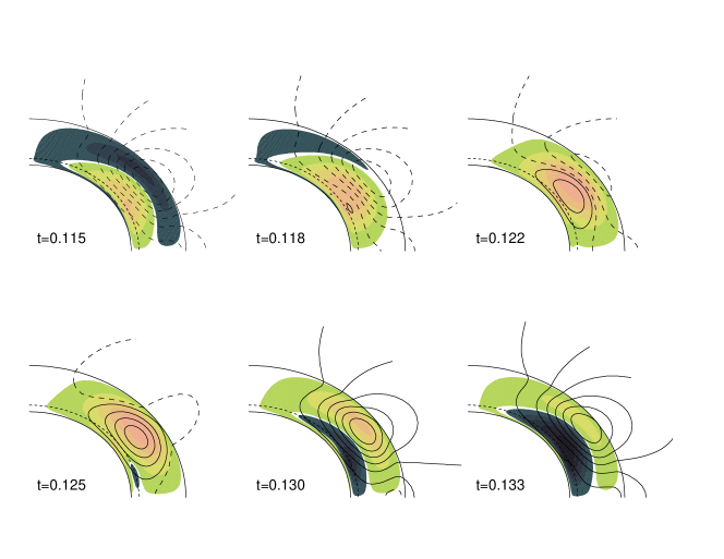
Figure 1: Model B of [2]. Snapshots of evolution of torioidal magnetic fileds (shadowed density plot) and poloidal fields (shown with streamlines) over the half of cycle.

Note, that our results are quite close to those in [2]. The small difference can be attributed to the difference in the method of solution of the problem.

The largest decay mode of the diffusion operator

Here, I give some details of the above computation within Maxima. The strongest side of the computer algebra system is that most of the computational work is done exactly. For example, all the derivatives in (7, 8) are computed directly by substitution of (9, 10) to (7, 8). The integration over space domain has to be done to proceed with the Galerkin method. This is carried out with help of the Gauss-Legendre procedure. The procedure is based on the so-called ”collocation points and weights” method. The collocation points are the set of zeros of the Legendre polynomial of the order $>N$ where $N$ is the number of the greatest mode among $n=1,\ldots N$ in (9, 10). The collocation points and weights can be found via subprogram ”pseudp.mac”. It is given in Appendix. The maxima session is started with the general definitions:

kill(all)$

batchload("pseudp.mac")$

(xb:0.,xe:1.)$

bftorat:true$

float2bf:true$

ratprint:false$

fpprec:64$

ratepsilon:1.e-32$

chn(x):=x$

realGr(L1,L2):=(if realpart(L1) >= realpart(L2) then true else false)$

Here, we find the collocation points and weights on radius,

(np:5,Nch:4*np,xchwh:gaulegP(-1,1,Nch,1), xch:xchwh[1],wh:xchwh[2])$

and on latitude,

(NT:6,NTT:6*NT,mut_w:gaulegP(-1,1,NTT,1),mut:mut_w[1],w:mut_w[2])$

Next, we define the indices for the basis functions and the parities for the toroidal and poloidal eigenmodes,

Nch:length(xch)$

NTT:length(mut)$

for m:1 thru NT do(   for n:1 thru np do(

        ki:np*(m-1)+n,ni[ki]:n,mi[ki]:m))$

ni:makelist(ni[i],i,1,NT*np)$

mi:makelist(mi[i],i,1,NT*np)$

NN:NT*np$

parity_b:0$

parity_a:0$

Note, that only a half of $[-1,1]$ intervals is used in computations. This leads to the computational economy and to increase the spectral resolution of the code. The following are the part of the code which defines the basis functions on radius ($S^{(B)}_{n}\rightarrow chtb_{n}$, $S^{(A)}_{nm}\rightarrow chta_{nm}$ ) and latitude,

kill(chtb1,chtb)$

chtb[n](x):=x*(legendre_p(1,x)-legendre_p(2*n+1,x))$

makelist(taylor(chtb[i](x),x,0,1),i,1,np)$

plot2d(makelist(chtb[i](x),i,1,np),[x,-1,1])$

kill(chta00)$

chta00(n,l,x):=x*(legendre_p(2*n+1,x)

  -((2*n+1)*(2*n+2)+2*l+2)*legendre_p(1,x)/(2*l+4))$

chta[n,l](x):=chta00(n,2*l-1,x),

kill(Pl10,Pla,Plb)$

Pl10(n,x):=expand((sqrt((2*n+1)/(2*n*(n+1)))*assoc_legendre_p(n,1,x)))$

Pla[n](x):=block(if parity_a=0 then bfloat(Pl10(2*n-1,x)) else bfloat(Pl10(2*n,x)) ) $

Plb[n](x):=block(if parity_b=0 then bfloat(Pl10(2*n-1,x)) else bfloat(Pl10(2*n,x)) ) $

As you see, we use odd or even associated Legendre polynomial in respective of the parity choice. To accelerate the integration procedure we calculate the matrices of basis functions over the sets of collocation points,

remarray(PLB,PLA)$

kill(PLB1,PLA1)$

PLB[n,i]:=bfloat(Plb[n](mut[i]))$

PLA[n,i]:=bfloat(Pla[n](mut[i]))$

PLA1[n,i]:=bfloat(Pla[n](mut[i])*w[i])$

PLB1[n,i]:=bfloat(Plb[n](mut[i])*w[i])$

CHTB[n,j]:=bfloat(chtb[n](xch[j]))$

CHTA[n,m,j]:=bfloat(chta[n,m](xch[j]))$

makelist(makelist(makelist(CHTA[n,m,j],n,1,np),m,1,NT),j,1,Nch)$

CHTB1[n,j]:=bfloat(chtb[n](xch[j])*wh[j])$

CHTA1[n,m,j]:=bfloat(chta[n,m](xch[j])*wh[j])$

makelist(makelist(makelist(CHTA1[n,m,j],n,1,np),m,1,NT),j,1,Nch)$

genmatrix(PLB,NT,NTT)$

genmatrix(PLA,NT,NTT)$

genmatrix(PLA1,NT,NTT)$

genmatrix(PLB1,NT,NTT)$

genmatrix(PLB2,NT,NTT)$

genmatrix(CHTB,np,Nch)$

genmatrix(CHTB1,np,Nch)$

Now we can to proceed to solution of the problem (7, 8). They can be treated separately. Firstly we define the left parts of (7,8),

kill(AA,BB)$

AA[ki,kj]:=bfloat(sum(CHTA1[ni[ki],mi[ki],j]*CHTA[ni[kj],mi[kj],j]*

    sum(PLA1[mi[ki],i]*PLA[mi[kj],i],i,1,NTT),j,1,Nch))$

BB[ki,kj]:=bfloat(sum(CHTB1[ni[ki],j]*CHTB[ni[kj],j]

    *sum(PLB1[mi[ki],i]*PLB[mi[kj],i],i,1,NTT),j,1,Nch))$

BB:genmatrix(BB,NN,NN)$

AA:genmatrix(AA,NN,NN)$

Note, the integration is just a product of sums over collocation points. Now lets compute the right part of (7). The computations are straightforward. The radial part is,

kill(CHTB_d2)$

CHTB_d2[n,j]:=bfloat(subst([x=xch[j]],

    expand((diff(diff(chtb[n](x),x),x) ))))$

genmatrix(CHTB_d2,np,Nch)$

kill(et_d)$

et_d[ki,kj]:=bfloat(sum(CHTB_d2[ni[kj],j]*CHTB1[ni[ki],j],j,1,Nch)

  *sum(PLB[mi[kj],i]*PLB1[mi[ki],i],i,1,NTT))$

et_d:genmatrix(et_d,NN,NN)$

The latitudinal part is computed as follows

kill(PLB_d2,PLB_d2m,PLB_d1,PLB_d)$

PLB_d2m[n,i]:=bfloat(subst([mu=mut[i]],expand((sqrt(1-mu^2)

    *diff(diff(sqrt(1-mu^2)*Plb[n](mu),mu),mu)))))$

genmatrix(PLB_d2m,NT,NTT)$

kill(er_d)$

er_d[ki,kj]:=bfloat(sum(CHTB1[ni[ki],j]*CHTB[ni[kj],j]/chn(xch[j])^2,j,1,Nch)

    *sum(PLB1[mi[ki],i]*PLB_d2m[mi[kj],i],i,1,NTT))$

er_d:genmatrix(er_d,NN,NN)$

Invert the left part of and solve the eigenvalue problem with help of lapack

BMI:invert_by_lu(BB)$

realGr0(L1):=(if realpart(L1) >=0 then true else false)$

load(lapack)$

MT:BMI.(er_d+et_d)$

lamb:(dgeev(MT,true))$

 

...

;; Loading #P"/usr/share/maxima/5.16.3/share/lapack/lapack/binary-cmucl/dtrevc.sse2f".

Now, lets sort the eigenvalues,

lmb:sort(flatten((col(lamb,1))[1]),realGr);

 

[- 20.19072855751148, - 48.83125052872499, - 59.68036461428608,

- 87.54250816953108, - 108.8085726200047, - 119.8731393320569,

- 135.9006458324267, - 169.2937978826357, - 193.7765731289586,

- 203.8596788530381, - 238.1199364033153, - 241.2729384729356,

- 260.8709651925637, - 277.930972796181, - 320.6253098224506,

- 328.0254017082749, - 373.0041226108443, - 410.8018157235754,

- 505.412713312208, - 577.4557504236772, - 665.4381736491396,

- 809.3382250971157, - 851.3024977594987, - 882.9750962899574,

- 932.6139588501989, - 970.2769707279747, - 1049.716092377411,

- 1259.650734653339, - 1830.07144488619, - 2585.672953057317]

The relevant spherical Bessel functions of the problem are

jn(n,x):=spherical_bessel_j(n,x)$

jnR(n,x):=x*spherical_bessel_j(n,x)$

Next we compute the first root of $j_{n}(x)$ and compare it with the first eigenvalue,

a1:find_root(jn(1,x),x,4,5)$

sqrt(abs(first(lmb)))-a1;

 

1.207158817351228e-10

Similarly, we solve (8). At the first, we invert the left part of it

AMI:invert_by_lu(AA)$

Then calculate the right part and apply lapack solver,

kill(CHTA_d2,PLA_d2)$

CHTA_d2[n,m,j]:=subst([x=xch[j]],(diff(diff(chta[n,m](x),x),x)))$

makelist(makelist(makelist(CHTA_d2[n,m,j],n,1,np),m,1,NT),j,1,Nch)$

PLA_d2[n,i]:=bfloat(subst([mu=mut[i]],(sqrt(1-mu^2)

    *diff(diff(sqrt(1-mu^2)*Pla[n](mu),mu),mu))))$

genmatrix(PLA_d2,NT,NTT)$

kill(ef_d)$

ef_d[ki,kj]:=bfloat(sum(CHTA_d2[ni[kj],mi[kj],j]

    *CHTA1[ni[ki],mi[ki],j],j,1,Nch)*

   sum(PLA1[mi[ki],i]*PLA[mi[kj],i],i,1,NTT)

  +sum(CHTA[ni[kj],mi[kj],j]*CHTA1[ni[ki],mi[ki],j]

    /chn(xch[j])^2,j,1,Nch)*

    sum(PLA1[mi[ki],i]*PLA_d2[mi[kj],i],i,1,NTT))$

ef_d:genmatrix(ef_d,NN,NN)$

MT:(AMI.ef_d)$

lamb:(dgeev(MT,true))$

Then, we sort the eigenvalues and compare the largest eigen mode with the first zero of $J_{1/2}(x)$,

lmb1:sort(flatten((col(lamb,1))[1]),realGr)$

float(sqrt(abs(first(lmb1)))-%pi);

 

- 9.681144774731365e-14

To compare the eigenfunctions we have to apply the scaling $S_{1}^{(B)}\left(.5\right)=1$ and $S_{1}^{(A)}\left(1\right)=1$.

The solution of dynamo problem is obtained in essentially the same way. I will put the code for it somewhere in the public place.

Appendix

The subroutine to find the collocation points and weghts for the polynomial order of n in interval $[x1,x2]$. The Newton method is applied,

load(orthopoly)$

orthopoly_returns_intervals:false$

fpprec:32$

float2bf:true$

ratprint:false$

load("linearalgebra")$

gaulegP(x1,x2,n):= block([xm,wm,A0,i,mm,pp,xm,xl,z,z1,numer,eps],

kill(xt,w), eps:1.e-16,fpprec:32,

(if oddp(n) then mm:(n+1)/2 else mm:n/2),

xm:0.5*(x2+x1), xl:0.5*(x2-x1),

for i: 1 while i <= mm do (

z:bfloat(cos(%pi*(i-0.25)/(n+0.5))),

do (pp:bfloat(n*(z*legendre_p(n,z)-legendre_p(n-1,z))/(z*z-1.0)),

z1:z,z:bfloat(z1-legendre_p(n,z)/pp),

if abs(z-z1) < eps

then return(z1)),

xt[i]:xm-xl*z1,

xt[n+1-i]:xm+xl*z1),

A:bfloat(genmatrix(lambda([i,j],legendre_p(i-1,xt[j])),n,n)),

RH:bfloat(transpose(matrix(

makelist((if i=1 then defint(legendre_p(0,x),x,-1,1) else 0),i,1,n)))),

w: bfloat(invert_by_lu(A) . RH),

return([makelist(xt[i],i,1,n),flatten(makelist(w[i],i,1,n))]))$

References

- [1] J. P. Boyd. Chebyshev and Fourie Spectral Methods. Dover: NY, 2001.
- [2] L. Jouve, A.S. Brun, R. Arlt, A. Brandenburg, M. Dikpati, A. Bonanno, P.J. Käpylä, D. Moss, M. Rempel, P. Gilman, M.J. Korpi, and A.G. Kosovichev. A solar mean field dynamo bechmark. Astron and Astrophys., 483:950–960, 2008.
- [3] P.W. Livermore and A. Jackson. A comparison of numerical schemes to solve the magnetic induction eigenvalue problem in a spherical geometry. Geophys. Astrophys. Fluid Dyn., 99:467–480, 2005.
- [4] V.V. Pipin and N. Seehafer. Stellar dynamos with effect Astron and Astrophys., in print, 2008.