Rings and spirals in barred galaxies. I Building blocks.

Abstract

In this paper we present building blocks which can explain the formation and properties both of spirals and of inner and outer rings in barred galaxies. We first briefly summarise the main results of the full theoretical description we have given elsewhere, presenting them in a more physical way, aimed to an understanding without the requirement of extended knowledge of dynamical systems or of orbital structure. We introduce in this manner the notion of manifolds, which can be thought of as tubes guiding the orbits. The dynamics of these manifolds can govern the properties of spirals and of inner and outer rings in barred galaxies. We find that the bar strength affects how unstable the $L_{1}$ and $L_{2}$ Lagrangian points are, the motion within the manifold tubes and the time necessary for particles in a manifold to make a complete turn around the galactic centre. We also show that the strength of the bar, or, to be more precise, of the non-axisymmetric forcing at and somewhat beyond the corotation region, determines the resulting morphology. Thus, less strong bars give rise to $R_{1}$ rings or pseudorings, while stronger bars drive $R_{2}$, $R_{1}R_{2}$ and spiral morphologies. We examine the morphology as a function of the main parameters of the bar and present descriptive two dimensional plots to that avail. We also derive how the manifold morphologies and properties are modified if the $L_{1}$ and $L_{2}$ Lagrangian points become stable. Finally, we discuss how dissipation affects the manifold properties and compare the manifolds in gas-like and in stellar cases. Comparison with observations, as well as clear predictions to be tested by observations will be given in an accompanying paper.

1 Introduction

Disc galaxies have a number of substructures, the most spectacular ones being their rings and their spirals. Barred galaxies, in particular, often have global spiral structure. They have two arms that often start from the ends of the bar and wind outwards covering a considerable region of the disc. In fact, global spiral structure is found more often in barred than in non-barred galaxies (e.g. Elmegreen & Elmegreen, 1989).

Rings also are often found in barred galaxies. They come in three varieties: nuclear rings, which are small and surround the nucleus, inner rings (r), which have the same size as the bar and are slightly elongated along it, and outer rings (R), which are considerably larger, with a major axis of the order of twice the bar size. Depending on their orientation with respect to the bar, outer rings are called $R_{1}$, when their major axis is perpendicular to the bar major axis, $R_{2}$, when their major axis is along the bar major axis, and $R_{1}R_{2}$, when they have a component parallel to the bar and a component perpendicular to it. The latter are less frequent than the previous varieties. Observational studies of their properties, including their frequencies, shapes and orientations, have been made by Buta (1995).

In order to understand the formation, evolution, and properties of any given structure it is essential to first understand its building blocks, i.e. the orbits that constitute it. This was clearly demonstrated in the case of bars, whose building blocks are closed periodic orbits elongated along the bar, generally called x₁ (Contopoulos & Papayannopoulos 1980, Athanassoula et al. 1983). The study of these building blocks provided answers to a number of crucial questions, like why bars are bisymmetric, why they rotate as rigid bodies, why they can not extend beyond corotation, why peanuts and boxy bulges form and what their structure and extent should be, etc. (Contopoulos 1981, Binney 1981, Pfenniger 1984, Skokos et al. 2002a, Patsis et al. 2002, Athanassoula 2005, etc.). Since bars are present in most disc galaxies, such studies went a long way towards explaining not only bar properties, but also bar formation and evolution, as well as the evolution of disc galaxies in general.

Spirals and rings, both inner and outer, also are present in a large fraction of disc galaxies. Identifying their building blocks will help explaining their formation and evolution, as well as their properties. It could also give information on the properties of the underlying disc galaxy and on the pattern speed and relative strength of the bar. For this purpose, we need to find the building blocks of spiral arms and of inner and outer rings in barred galaxies and to study their properties. Of course such a study is only a step towards understanding a given structure, since it neglects collective effects which can play an important role. Yet it can provide a full physical understanding. It is this first step that is the aim of our work. We started it in two previous papers (Romero-Gómez et al. 2006, hereafter Paper I, and Romero-Gómez et al. 2007, hereafter Paper II), while a more analytical approach to the problem can be found in Romero-Gómez et al. (2008).

In Papers I and II we proposed a theory which can explain the formation of both rings and spirals in barred galaxies using a common framework. It is based on the chaotic orbital motion driven by the unstable equilibrium points of the rotating bar potential. We thus suggested that spirals, rings and pseudorings are related to the invariant manifolds associated to the periodic orbits around these equilibrium points and, particularly, to the existence of heteroclinic or homoclinic orbits. Thus, $R_{1}$ rings are associated to the presence of heteroclinic orbits, while $R_{1}R_{2}$ are associated to the presence of homoclinic orbits. Spiral arms and $R_{2}$ rings, however, are present when there exist neither heteroclinic nor homoclinic orbits. To establish this link, we calculated both manifolds and their associated trajectories in a large number of cases, covering the relevant parameter space of three simple barred galaxy models. This allowed us to discuss the formation of different morphological structures according to the properties of the galaxy models. Work along similar lines has also been carried out by other teams. Danby (1965) argued that bar orbits departing from the vicinity of the unstable Lagrangian points play an important role in the formation of the spiral arms. Kaufmann & Contopoulos (1996) linked chaotic orbits to the presence of spiral arms. This was further developed by Patsis (2006) with the help of response calculations in the potential of NGC 4314, as calculated by Quillen, Frögel & Gonzalez (1994), and by Voglis, Stavropoulos & Kalapotharakos (2006) who used a potential from an $N$-body simulation. Manifolds were specifically referred to, although in a quite different way from that used in our work, by the late Prof. Voglis and his collaborators (Voglis, Tsoutsis & Efthymiopoulos, 2006).

The above cited works were crucial in establishing the importance of chaos in the formation of spirals and rings in barred galaxies and, more specifically, the role of the manifolds. Yet a considerable amount of work still needs to be done, particularly in the practical aspects, since a number of crucial questions are still unanswered. Which properties of the manifolds influence most those of rings and spirals? Which properties of the galactic potential determine whether the morphology will be that of a ring or that of a spiral? In other words, is it possible from the barred galaxy potential to predict the galaxy morphology? If yes, this would be a clear prediction and therefore a test of our theory. How does the morphology of the manifolds compare with those of observed spirals and rings? Are such manifolds to be always expected, or are there cases where the unstable Lagrangian points can somehow become stable? What happens to the manifolds in such cases? We attempt to answer these questions in this paper (Paper III of this series).

In section 2 we give a simplified and physical description of the main theoretical tools necessary for this study. We describe here the Lagrangian points, the invariant manifolds and their associated orbits. Section 3 links manifold morphologies to bar properties. Section 4 introduces some useful properties of the invariant manifolds. Section 5 addresses the option of stable $L_{1}$ and $L_{2}$ Lagrangian points and discusses the type of morphologies this would entail. Section 6 discusses gas and compares its response morphology to that of manifolds. We briefly summarise in section 7. Comparison with observations will be presented in Paper IV of this series, where we will also give a global discussion on the applicability of our theory and a brief comparison with other spiral structure theories.

2 Theoretical basis

In this section we summarise the main theoretical tools necessary for our study. Our description aims towards a physical understanding and is thus wilfully somewhat simplified. A more accurate and thorough description is given in Papers I and II and in the references therein, while some analytical intricacies of manifolds in a simplified, rotating, non-axisymmetric potential have been presented by Romero-Gómez et al. (2008).

2.1 General

As in the two previous papers, we use here simple, rigid models, since these contain all the basic, necessary physics. They are composed of an axisymmetric part and of a bar rotating with a constant angular velocity, which we will refer to as the pattern speed. We concentrate on the motion on the $z$ = 0 plane (equatorial plane of the galaxy), since the motion in the vertical direction can be essentially described by an uncoupled harmonic oscillator, is assumed to be of relatively small amplitude and does not affect the motion in the $z$ = 0 plane (Paper I). We also limit ourselves to bars rotating in the direct sense, i.e. here counter-clockwise, in agreement with all observational and simulation results. We will work in a frame of reference rotating with the bar, i.e. in which the bar is at rest, since the dynamics are much easier described there (Binney & Tremaine, 2008). We use the convention that, in this frame, the bar is along the $x$ axis.

We consider three different barred galaxy models, described in Appendix A. They consist of an axisymmetric component and a rigid, non-evolving bar, rotating with a constant angular velocity $\Omega_{p}$. Model A has a Ferrers’ bar (Ferrers, 1877), characterised by its semi-major axis $a$, its axial ratio $a/b$ and its quadrupole moment $Q_{m}$. Our fiducial case all through this paper is a typical example of a model with a Ferrers’ bar and has $a=5$, $a/b=2.5$, $r_{l}=6$, $Q_{m}=4.5\times 10^{4}$, $\rho_{c}=2.4\times 10^{4}$ and $n=1$, all in the units given in Appendix A. Here $r_{L}$ is the Lagrangian radius, $\rho_{c}$ is the central concentration of the system and $n$ is the index of the Ferrers’ bar (Appendix A). Our conclusions, however, are based on a large number of such models, covering a wide range of parameters.

Models D and BW have ad hoc formulae for the bar potential and were initially given by Dehnen (2000) and by Barbanis & Woltjer (1967), respectively. Their bar strength is quantified with the free parameters $\epsilon$ and $\hat{\epsilon}$, respectively. They can have a much stronger non-axisymmetric forcing beyond corotation than models A, and are meant to represent and include forcings not only from bars, but also from spirals, from oval discs and from triaxial haloes. We have kept all these forcings bar-like, i.e. we have not included any radial variation of the azimuthal dependence. This was done on purpose, in order not to bias the response towards spirals and in order to avoid the extra degree of freedom resulting from the azimuthal winding of the force.

2.2 Equilibrium points and Lyapunov orbits

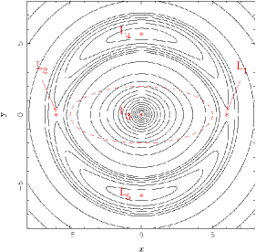
Figure 1: Contours of constant effective potential. The values of the iso-effective potentials have been chosen so as to show best the relevant dynamical features. The outline of the bar is given by a dashed line and the five Lagrangian points are marked by asterisks.

For barred galaxy models such as those used here, the energy of a particle in the rotating frame is a constant of the motion and is often referred to as the Jacobi constant, $E_{J}$, or simply as the energy (Binney & Tremaine, 2008). A useful quantity to define here is the effective potential,

$$\Phi_{\hbox{\scriptsize eff}}=\Phi-\frac{1}{2}\Omega_{p}^{2}\,(x^{2}+y^{2}),$$

which can be thought of as the potential in the rotating frame of reference. $\Omega_{p}$ is the bar pattern speed, i.e. the angular velocity with which the bar rotates, assumed constant, and $\Phi$ is the potential. The curve $\Phi_{\hbox{\scriptsize eff}}=E_{J}$ is called the zero velocity curve (ZVC). All regions in which $\Phi_{\hbox{\scriptsize eff}}>E_{J}$ are forbidden to particles with Jacobi constant equal to $E_{J}$ or less, and are therefore called forbidden regions.

The motion has five equilibrium points, i.e five points where

$$\frac{\partial\Phi_{\hbox{\scriptsize eff}}}{\partial x}=\frac{\partial\Phi_{\hbox{\scriptsize eff}}}{\partial y}=0.$$

They are often called the Lagrangian points $L_{i}$, $i$ = 1, .. 5 and their location is shown in Fig. 1. $L_{3}$ is at the origin of the coordinates, $L_{4}$ and $L_{5}$ lie on the direction of the bar minor axis, symmetrically with respect to the centre, and $L_{1}$ and $L_{2}$ lie on the direction of the bar major axis, also symmetrically with respect to the centre. For realistic bar potentials, the distance of the $L_{4}$ and $L_{5}$ from the centre is somewhat larger than that of the $L_{1}$ and $L_{2}$ (Athanassoula, 1992a). We will refer to the distance of the $L_{1}$ and $L_{2}$ from the centre as the Lagrangian radius $r_{L}$. The $L_{4}$ and $L_{5}$ are maxima of the effective potential, $L_{3}$ is a minimum and $L_{1}$ and $L_{2}$ are saddle points, i.e. there

$$\frac{\partial^{2}\Phi_{\hbox{\scriptsize eff}}}{\partial x^{2}}<0,~{}~{}\frac{\partial^{2}\Phi_{\hbox{\scriptsize eff}}}{\partial y^{2}}>0.$$

$L_{3}$ is stable and is surrounded by the x₁ family of periodic orbits (Contopoulos & Papayannopoulos, 1980), which are the backbone of the bar (Athanassoula et al. , 1983). $L_{4}$ and $L_{5}$ are also generally stable and each one of them is surrounded by a family of periodic orbits, called the banana orbits because of their shape. These three Lagrangian points and the corresponding families of periodic orbits have been studied extensively (see Contopoulos, 2002, and references therein). $L_{1}$ and $L_{2}$ are generally unstable and are surrounded by a family of periodic orbits, often called the Lyapunov orbits (Lyapunov, 1949). These orbits have a roughly elliptical shape, their size increases with energy and they are unstable, becoming stable only at energies much higher than that of $L_{1}$ and $L_{2}$ (Skokos et al. , 2002a). An example is shown in Fig. 2. The dynamics of the $L_{1}$ and $L_{2}$ points and of the Lyapunov family of periodic orbits had been little studied before we started on Paper I, presumably because, being unstable, they were deemed less interesting. Yet, as we showed in Papers I and II and will further stress here, the manifolds they generate can account for the spirals, as well as for the inner and outer rings observed in barred spirals.

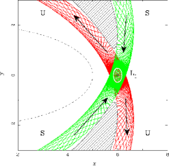
Figure 2: Dynamics of the region around $L_{1}$ for a typical value of the energy. The location of $L_{1}$ is given by an asterisk and we show in a white solid line the corresponding Lyapunov orbit around it. The two branches of the unstable invariant manifold (marked $U$ and plotted with red lines), and the two branches of the stable invariant manifold (marked $S$ and plotted with green lines) are for the same value of the energy. The arrows give the direction of the motion along the manifold and the hatched areas are the forbidden regions surrounded by the zero velocity curves (solid black lines). The loci of the manifolds in the vicinity of $L_{2}$ is identical, but mirrored with respect to the bar minor axis. The outline of the bar is given by a black dashed line. All through this paper and wherever a distinction is necessary, the unstable manifolds will be plotted in red and the stable ones in green.

Since the Lyapunov orbits are unstable, they can not trap around them any regular orbits, so that any orbit with initial conditions in their vicinity in phase space will not stay near them. The time it takes for the orbit to leave the vicinity (in the phase space sense) of the corresponding Lyapunov periodic orbit depends on its Jacobi constant. For lower values of the energy, i.e. values near that of $L_{1}$, the Lyapunov orbits have a smaller extent and are more unstable. Thus, any orbit starting from their immediate vicinity in phase space will escape their neighbourhood quite fast, in a time corresponding to a couple of bar rotations. For larger values of the energy, the Lyapunov orbits become larger and more asymmetric and they are less unstable, so that the orbits starting from their immediate vicinity in phase space will take longer to escape.

2.3 Invariant manifolds and associated orbits

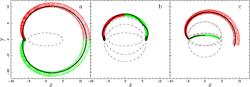
Figure 3: Examples of homoclinic (a), heteroclinic (b) and escaping (c) orbits (black thick lines) in the configuration space. In red, we plot the unstable invariant manifolds associated to these orbits, while in green we plot the corresponding stable invariant manifolds. In dashed lines, we give the outline of the bar and, in (b) and (c), we plot in dot-dashed lines the zero velocity curves of the same energy as the orbits and manifolds.

Since any orbit in the immediate vicinity (in phase space) of the unstable Lyapunov orbits can not stay trapped around them, it will have to escape the neighbourhood of the corresponding Lagrangian point. Not all departure directions are, however, possible. Let us consider a Lyapunov orbit of a given energy and another orbit of the same energy and initially very close in phase space to the Lyapunov one. The direction in which this orbit escapes is set by what is called the invariant manifolds. We can simply think of the manifolds as tubes which guide the orbits escaping from the vicinity of the Lagrangian points, so that these manifolds/tubes are filled and surrounded by orbits. We refer the reader to Paper I and to the references therein for a precise definition and for a description of how we calculate the manifolds in practise.

Fig. 2 explains the dynamics around the $L_{1}$ Lagrangian point for a typical value of the energy. We plot here (in white) the Lyapunov orbit of that energy and the four branches of the invariant manifold that emanate from it, two inner and two outer. For two of them, one inner and one outer, the motion is away from the region of the Lyapunov orbit and they are referred to in the theory of dynamical systems as the unstable branches of the manifold. For the other two – again one inner and one outer – the motion is towards the Lyapunov orbit and they are referred to in the theory of dynamical systems as the stable branches of the manifold. We will use these terms here also, but we want to stress that this does not mean that the orbits that are guided by these branches are also stable or unstable, respectively. In fact these orbits are all chaotic, but they are in a loose way ‘confined’ by the manifolds, so that they stay together in what could be described as a bundle, at least for a couple of rotations around the bar. In that sense, the manifolds can be thought of as driving the dynamics in the vicinity of the $L_{1}$ and $L_{2}$,

Fig. 2 shows only the vicinity of the Lagrangian point, but, as can be seen in Fig. 3, the manifolds extend far beyond this neighbourhood. They can thus be responsible for more global structures in the galaxy. It should, however, be stressed that not all particles can be affected by the manifold dynamics, but only those in a relatively narrow energy range, whose lower limit, as described in Paper I, corresponds to the energy of the $L_{1}$ and $L_{2}$ points. Since two of the manifold branches have motions inwards and two outwards, manifolds can play a crucial role in the transport of material between different parts of the galaxy. Loosely, they can be thought of as gates between the regions within and the regions outside corotation (as in astrodynamics, see Koon et al. 2000, Gomez et al. 2004).

The morphology of the manifolds with respect to the Lagrangian points allows us to classify their outer branches in three types, homoclinic, heteroclinic and escaping. This is illustrated in Fig. 3, where we show, for each case, the manifolds and a corresponding orbit. All depart from an unstable Lyapunov periodic orbit around one of the unstable equilibrium points, in this case $L_{2}$. We define as homoclinic the manifolds and orbits that return to it (Fig. 3a). Similarly, heteroclinic manifolds and orbits are those that approach the corresponding Lyapunov periodic orbit around the Lagrangian point at the opposite end of the bar, $L_{1}$ (Fig. 3b). Finally, there are manifolds and orbits that do not return to either $L_{1}$ or $L_{2}$, but spiral outwards from the region of the unstable Lyapunov periodic orbits to reach the outer regions of the galaxy. Following the notation of Paper II, we refer to them as escaping. This means that they can reach regions far from the vicinity of the bar, but not that they can escape to infinity. They correspond to the unstable branches of the manifold and the motion along them is outwards and in the clockwise (retrograde) sense. Similarly to the escaping manifolds and orbits, there are incoming manifolds and orbits, which, coming from the outer parts of the galaxy, reach the vicinity of $L_{1}$ or $L_{2}$. They correspond to the stable branches of the manifold and their loci can be obtained from the unstable ones after a reflection with respect to the bar major axis. The motion along them is inwards and anticlockwise (direct). These, however, as we will show in Paper IV, do not have any physical significance in our problem, so we will not discuss them much.

There is a further crucial difference between the homoclinic and heteroclinic cases on the one hand, and the escaping ones on the other. In the former the stable and unstable branches overlap, at least partly, both in configuration space (positions) and in phase space (position, velocity space). The contrary is true for the latter. Thus, in the former cases orbits can be trapped (guided) by both the stable and the unstable branches of the manifold simultaneously. This is, for example, the case for the two orbits plotted by solid black lines in the left and middle panels of Fig. 3. This, however, is not the case for the orbit in the right panel, which belongs to the unstable manifold exclusively. In this sense, the red and green colours in the left and middle panels are arbitrary, since any part of the manifold/orbit can be assigned to both the stable and the unstable branches.

We will argue here that the three types of orbits we presented here – i.e. the homoclinic, the heteroclinic, and the escaping orbits – are the backbone of ringed structures and of spiral arms observed in disc galaxies, in the same way as x₁ orbits are the backbone of the bar.

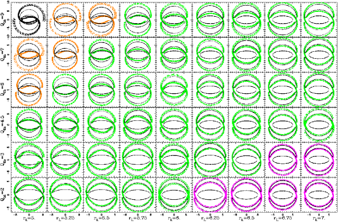
Figure 4: Effect of the bar strength and of the Lagrangian radius $r_{L}$ on the manifold loci for model A. The strength of the bar is parametrised by the quadrupole moment $Q_{m}$. Each panel corresponds to a pair of ($Q_{m}$, $r_{L}$) values, given on the left (in units of 10⁴) and on the bottom of the figure, respectively. The remaining parameters are as in the fiducial model. The manifolds are plotted in a colour which is determined by their morphology: green for $R_{1}$, orange for $R_{1}^{\prime}$ and black for spirals (see text for lilac). The black dotted lines give the outline of the bar and the zero velocity curves of the same energy as the manifolds.

Two more points need to be made here. One is that the manifolds and orbits we present here are only the building blocks, but do not in any way assure us that the corresponding structure will be present in the galaxy. Indeed a given manifold may exist, but may not trap any orbits, so that the corresponding structure will not be visible in the galaxy. This is similar to the periodic orbits, which are the building blocks of bars and which need to trap regular orbits around them, for the bar to form. In other words, the existence of a manifold is a necessary, but not a sufficient condition for the corresponding galactic structure to form.

The second point we wish to stress is that the orbits guided by the manifolds are not the only ones in the relevant galactic regions. On the contrary, there are a number of other possible orbits. For example, there are families of periodic orbits beyond corotation (e.g. the x${}_{1}^{\prime}$ in the notation of Contopoulos & Papayannopoulos (1980) and the A’, B’, -2/1 and -1/1 in the notation of Athanassoula et al. (1983)) that can have large stable parts so that the corresponding periodic orbits can trap regular orbits around them. It is the ensemble of these orbits, those driven by the manifolds and those trapped around the stable periodic orbits, that will structure the region beyond corotation. Here we concentrate on the manifold-driven orbits in order to propose them as possible building blocks for spirals and rings.

3 manifold morphologies and bar properties

How does the shape of the outer manifold loci depend on the parameters determining the bar potential? To answer this question we calculated manifolds in a very large number of models from all three families of potentials and include some of the manifold loci in Figs. 4 to 6. Fig. 4 corresponds to models of type A, Fig. 5 to models of type D and Fig. 6 to models of type BW.

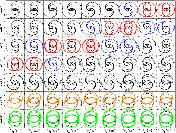
Figure 5: As for Fig. 4, but for D type models. The parameter $\epsilon$ is a measure of the bar strength. $R_{2}$ rings are plotted in blue and $R_{1}R_{2}$ in red.

Models of type A have 4 main free parameters : their central concentration $\rho_{c}$, their bar axial ratio $a/b$, their quadrupole moment $Q_{m}$ and their pattern speed parametrised by the value of the Lagrangian radius $r_{L}$. As we showed in Paper II, two of these, the central density $\rho_{c}$ and the axial ratio $a/b$, influence the potential mainly within corotation, so that we do not need to consider their effect in depth here. The other two, $Q_{m}$ and $r_{L}$, influence strongly the manifold loci also beyond corotation, so we will mainly limit our discussion to them. Contrary to Paper II, where we only presented the manifold shapes for barred galaxy models on the axes of this parameter space, we will consider here a grid of relevant values for these parameters. In this way we can get a much better insight of the dependence of the manifold morphology on the bar properties. The other two families of models, D and BW, have only two free parameters, the first one ($\epsilon$ or $\hat{\epsilon}$, respectively) linked to the bar strength, and the second one ($r_{L}$) being the Lagrangian radius. We will thus for each of the models present a composite two-dimensional plot including many models. Each row corresponds to a given value of the bar strength, and each column to a given value of the pattern speed. In fact, both of these parameters influence the strength of the non-axisymmetric forcing at and somewhat beyond the corotation radius.

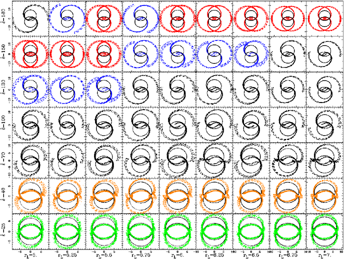
Figure 6: As for Fig. 5, but for BW type models. The parameter $\hat{\epsilon}$ is a measure of the bar strength.

We classified the morphologies of the outer manifold branches into spirals (black), $R_{1}$ rings (light green), $R_{1}$ pseudorings (orange), $R_{2}$ rings and pseudorings (blue) and $R_{1}R_{2}$ rings and pseudorings (red). For model A, we plot in lilac cases with $rR_{1}$ morphology, but which have a ratio of inner to outer major axes which does not seem compatible with observations. The ones corresponding to the the smallest bar strengths have two rings with diameters which do not differ much. In cases where the bar amplitude is so low, the motion in this region may be almost independent of the bar, i.e. governed more or less by the axisymmetric mass distribution. In such cases, once self-gravity is taken into account, the two rings could merge, giving rise to a thicker, single, very low amplitude feature.

How is this classification done? For the models, it is possible to use the presence of homoclinic, heteroclinic and escaping manifolds and orbits in order to classify the morphologies. This, however, has not been done by observers classifying real galaxies, who use eye classification. Since we wish to make extensive comparisons with observations in Paper IV, we will use the same classification means as observers. In general, it is easy to differentiate by eye between the different types of morphology; borderlines cases, however, are a matter of personal judgement. There are such borderline cases between $R_{1}$ and $R_{1}^{\prime}$, between $R_{1}^{\prime}$ and spirals, etc. This should be taken into account when assessing any of the results obtained here and when discussing statistical results in Paper IV.

Figures 4 to 6 reveal a very clear trend. Namely the different morphologies are not randomly distributed in the (strength, Lagrangian radius) plane, but, on the contrary, different morphologies are grouped together in different parts of that plane, which, in a very rough way, can be seen as diagonal stripes. $R_{1}$ rings occupy the bottom right, followed by spirals, then by $R_{2}$ and $R_{1}R_{2}$ and finally by more $R_{2}$ and spirals.

This clearly indicates that the morphology depends on the strength of the non-axisymmetric forcing in the part of the galaxy occupied by the manifolds. Indeed, the bar strength increases from the bottom to the top row. The pattern speed, however, also influences the bar strength in that region. As the pattern speed decreases (i.e. as the Lagrangian radius $r_{L}$ increases) the distance between the end of the bar and the $L_{1}$ (or $L_{2}$) increases, so that the manifolds will occupy a region farther away from the bar, i.e. a region which has a weaker non-axisymmetric forcing. Thus, the influence of the bar is stronger as we move towards stronger bars (bottom to top in each figure) and as the pattern speed increases (right to left in each figure).

In the language of dynamical systems, Figs. 4 to 6 show that the strength of the perturbation in the region of the manifolds determines whether these are homoclinic, heteroclinic, or of escaping type (Fig. 3). Alternatively, in more astronomical terms, these plots argue that the strength of the bar in the region beyond but close to corotation should determine whether we will have spirals or rings, and more specifically what type of rings.

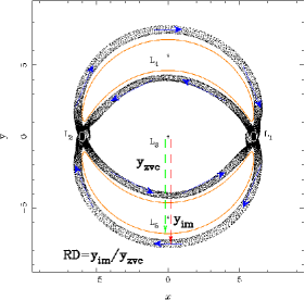
Figure 7: Example of a manifold with $rR_{1}$ morphology (black). The sense of circulation of material along it is shown by blue arrows. The ZVC of the same energy is shown in orange. The distance from the centre of the galaxy to the outer part of the ZVC ($y_{ZVC}$) and the distance from the centre of the galaxy to the outer branch of the manifold ($y_{im}$), both measured along the $y$ axis, are marked by dashed arrows in green and red, respectively. Their ratio, $RD=y_{im}/y_{ZVC}$, is used in Fig. 8 to delimit the various morphologies.

To distinguish further between the different types of responses we introduce two relevant quantities. The first one quantifies the relative bar strength in the region of $L_{1}$. For this we use a standard measure of the bar strength at a given radius, namely

$$Q_{t}(r)=(\partial\Phi(r,\theta)/\partial\theta)_{max}/(r\partial\Phi_{0}/\partial r),$$ (1)

where $\Phi$ is the potential, $\Phi_{0}$ is its axisymmetric part and the maximum in the numerator is calculated over all values of the azimuthal angle $\theta$. We calculate $Q_{t}(r)$ at the radius of $L_{1}$, i.e. at $r=r_{L1}$ and denote it by $Q_{t,L_{1}}$. The choice of the second relevant quantity is motivated by the results in Sect. 4. More specifically, we will show in that section that, in the cases where $L_{1}$ and $L_{2}$ are weakly unstable, the loci of the manifolds are located very near the zero velocity curve of the same energy, while, in the strongly unstable case, they depart considerably from it. We quantify this by measuring on the $y$ axis the ratio of two distances, namely the distance between the centre of the galaxy and the manifold ($y_{im}$ in Fig. 7) and the distance between the centre and the outer branch of the corresponding ZVC ($y_{ZVC}$ in Fig. 7). We refer to this ratio ($y_{im}$/$y_{ZVC}$) as $RD$. As will be shown in Sect. 4, both quantities $Q_{t,L_{1}}$ and $RD$ measure the bar strength, albeit in a different way.

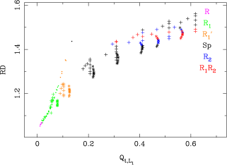
Figure 8: Location of the models shown in Figs 4 to 6 in the ($RD$, $Q_{t,L_{1}}$) plane. $RD$ is the ratio of $y_{im}$ (the distance from the centre of the galaxy to the outer branch of the manifold) to $y_{ZVC}$ (the distance from the centre to the branch of the corresponding ZVC farthest from the centre). $Q_{t,L_{1}}$ is a measure of the bar strength at the radius of the $L_{1}$, given by eq. (1). The various morphologies – $R_{1}$, $R_{1}^{\prime}$, spirals, $R_{2}$ and $R_{1}R_{2}$ – are noted by symbols of different colour, as given in the figure. The various symbols show whether the model is A (dots), D (crosses), or BW (asterisks).

With the help of these two quantities we can include the main information in a single plot, given in Fig. 8. This shows the location of all models from Figs 4 to 6 on the ($Q_{t,L_{1}}$, $RD$) plane and reveals that the different types of morphologies are segregated on different parts of this plane, independent of the type of the model. For the lowest $Q_{t,L_{1}}$ values (roughly $Q_{t,L_{1}}<0.1$) we have only $R_{1}$ outer rings, while somewhat higher values (roughly in the region $0.1<Q_{t,L_{1}}<0.2$) give $R_{1}^{\prime}$ morphologies. Yet higher values give spirals and $R_{2}$ and $R_{1}R_{2}$ rings. Fig. 8 shows that there is no division between these three types by $Q_{t,L_{1}}$ value alone, but that there is one, albeit a bit rough, by the value of $RD$.

Following the location of the models on the ($Q_{t,L_{1}}$, $RD$) plane, after the $R_{1}$ and the $R_{1}^{\prime}$ we find spirals, followed by $R_{2}$ rings and pseudorings, then $R_{1}R_{2}$, then again $R_{2}$ and again spirals. This second group of spirals has much more open arms than the first one.

We redid this plot, using, instead of the value of $Q_{t,L_{1}}$, the average value of $Q_{t}$ in an annulus of given width starting at $L_{1}$ and extending beyond it and found qualitatively the same results for a wide range of widths. It is important to underline that this plot includes three different types of bar potentials, which are widely different. Thus, Fig. 8 argues that the morphological segregation exists for many, if not all, reasonable bar potentials. It also shows, together with Figs. 4 to 6, that a spiral forcing is not mandatory in order to obtain a spiral response, but that a spiral can be obtained with a purely bar or bar-like forcing, provided of course this is sufficiently strong in the regions beyond corotation. This has been already shown to be the case for the density wave theory (e.g. Feldman & Lin, 1973; Athanassoula, 1980). It is nevertheless true that it is easier to obtain a spiral response with a spiral than a with a bar forcing. It is also clear that if one adds a spiral forcing to the bar one, it will be even easier to obtain spirals, as underlined already by Lindblad, Lindblad & Athanassoula (1996), in their modelling of NGC 1365. Thus, for bar plus spiral non-axisymmetric forcings spirals will form for lower relative strength than for the bar-only case. Therefore, the exact delimitation between spirals and rings in e.g. Fig. 8 will depend on whether the forcing is bar only, or bar plus spiral.

4 Further properties of the invariant manifolds

We saw in Sect. 2.2 that the Lagrangian points $L_{1}$ and $L_{2}$ are generally unstable, but we still need to quantify how unstable they are. For this we use a positive quantity $\lambda$, introduced and defined in appendix B. The larger numerical values of $\lambda$ correspond to more unstable $L_{1}$ and $L_{2}$ Lagrangian points.

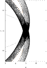
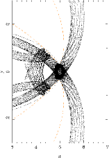
Figure 9: Invariant manifolds in the immediate neighbourhood of $L_{1}$ for a strongly unstable case (right panel) and for a weakly unstable one (left panel). More than one revolution is shown for the inner manifold branches. The dot-dashed black lines show the bar outline and the the dashed orange ones the zero velocity curves.

Fig. 9 shows the invariant manifolds in the immediate neighbourhood of $L_{1}$ for a strongly unstable case and for a weakly unstable one. We chose as examples a model with a strong bar ($Q_{m}$ = 9, right panel of Fig. 9) and with a weak bar ($Q_{m}$ = 0.5, left panel of Fig. 9), both with $r_{L}$ = 5. These models have $\lambda$ = 62.85 and $\lambda$ = 11.88, respectively. There are several clear differences, revealing how the strength of the bar influences the instability of the $L_{1}$ and $L_{2}$ and the manifold properties. As can be seen in Fig. 9, in the weakly unstable case (left panel) a considerable part of the motion is perpendicular to the main extent of the manifold, so that the manifolds are more densely packed and $T_{f}$, the time necessary for them to perform half a revolution around the galaxy centre, is very long. On the contrary, for a strongly unstable case (right panel) most of the motion is along the main extent of the manifolds, so that the manifolds are less densely packed and $T_{f}$ is much shorter.

This is illustrated in Fig. 10, which shows the time $T_{f}$ necessary for the outer branch of a manifold starting from the immediate neighbourhood (in phase space, see Paper I) of a Lyapunov periodic orbit to perform half a revolution around the galactic centre, as a function of the quadrupole moment, $Q_{m}$, of the bar. The remaining parameters are those of the fiducial A model (Sect. 2.1). Calculating the corresponding $\lambda$ values for each of the barred potentials, we see that, as expected, stronger bars make more unstable Lagrangian points. We place the corresponding values of $\lambda$ on the upper limit of the plot, to show how $\lambda$ depends on $Q_{m}$ and also how $T_{f}$ depends on $\lambda$. Fig. 10 shows clearly that $T_{f}$ drops very fast with increasing bar strength, in an exponential-like way.

Figure 10: $T_{f}$, i.e. the time necessary for the outer branch of a manifold starting from the immediate neighbourhood (in phase space) of a Lyapunov periodic orbit to perform half a revolution around the galactic centre, as a function of $Q_{m}$ (the quadrupole moment of the bar, lower abscissa) and of the $\lambda$ parameter measuring the instability of the Lagrangian point (upper abscissa). $T_{f}$ is measured in units of the bar rotation period and $\Omega_{p}$ is the bar pattern speed. This figure shows clearly that strong bars (i.e.bars with large $Q_{m}$ values) have more unstable $L_{1}$ ($L_{2}$) Lagrangian points (i.e. larger $\lambda$ values) and develop their manifolds in shorter times.

This is not the only difference. As can be seen in Fig. 9, the loci of the manifolds in the weakly unstable case are located very near the zero velocity curve of the same energy, contrary to the manifolds of the strongly unstable case, which are at a considerable distance from it. Moreover, Figs. 4 to 6 show that this is true not only in the vicinity of $L_{1}$, or $L_{2}$, but also over all their extent. Thus, after a rotation of 90^∘ the manifolds of the weakly unstable cases are much nearer to the centre than those of the strongly unstable cases. This conditions the shape of the manifold loci and explains the result found in Sect. 3.

Figure 11: Angle between the direction of the manifold near the Lagrangian point and the direction of the bar major axis, plotted as a function of $Q_{m}$ (the quadrupole moment of the bar, lower abscissa) and of the $\lambda$ parameter measuring the instability of the Lagrangian point (upper abscissa). Strongly unstable configurations have large values of $\lambda$ and smaller values of the angle.

Another way of seeing this is by measuring the angle between the direction of the outer manifold branches near $L_{1}$ and the direction of the bar major axis. For weakly unstable cases – as in the left panel of Fig. 9 – this angle is large, tending to $90^{\circ}$ as the $L_{1}$ and $L_{2}$ become less and less unstable. On the contrary, this angle is smaller in the case of strongly unstable Lagrangian points. This is illustrated in Fig. 11, which plots this angle as a function of $Q_{m}$ (lower abscissa) and $\lambda$ (upper abscissa), for the same models as in Fig. 10.

There are yet further differences. Weak bars drive particles on heteroclinic orbits (see Sect. 2.3) and produce the shape of $rR_{1}$ rings and pseudorings (see Sect. 3). The circulation of the material within the manifolds is shown in Fig. 7. Four different paths are possible. Material can circulate along the inner branches of the manifold (i.e. keeping within the inner ring), or along the outer manifold branches (i.e. keeping within the outer ring), or have a mixed trajectory. The latter is particularly interesting. Mass circulates within the manifolds, moving from $L_{1}$ along the inner ring (inner branches of the manifold) to the vicinity of the $L_{2}$ and from there outwards on the outer ring (i.e. on an outer branch of the manifold) until it reaches a maximum distance from the centre. At this point the radial component of the velocity changes sign and mass elements will move inwards, still keeping on the outer branch of the manifold, back towards the Lagrangian point $L_{1}$. This closes one complete circulation path. This path and the direction of motion along it are shown in Fig. 7. There are two such paths, one above and one below the $x$ axis, symmetric with respect to the bar major axis. The four circulation paths can be repeated or alternated. For all four, there is no net inwards or outwards motion. Material, however, circulates within the galaxy, so that there is a radial, as well as azimuthal mixing. In particular, for the paths involving both inner and outer branches, material circulates from the region within corotation to the region outside it and vice versa. Initially, matter is trapped in these manifolds at the time the bar is formed, while further material is added as the bar strength increases.

For very strongly unstable $L_{1}$ and $L_{2}$, the situation is different. Material now follows escaping orbits, which trace the spirals. The stable and unstable manifolds intersect in the configuration space [the ($x$, $y$) space], but not in phase space [i.e. not in the (position, velocity) space]. Indeed, on the $y$ axis, where the stable and unstable branches intersect in the configuration space, the radial velocity component of the particles driven by the unstable branch is outwards, while that of particles on the stable branch is inwards (note that at this point the radial component of the velocity was equal to zero for the heteroclinic case). Thus, particles initially trapped in the inner branches of the manifold will move towards one of the unstable Lagrangian points, say the $L_{2}$, and from there outwards guided by an unstable outer branch of the manifold. Contrary to the case of homoclinic, or heteroclinic manifolds and orbits, they will not come back to $L_{1}$ or $L_{2}$, Thus the motion along first the inner stable manifold and then the outer unstable manifold will take mass from the outer region of the bar, which is a high density region in the galaxy, and feed it into the spiral. This will bring a redistribution of matter within the galaxy and a net outwards motion. Of course, in principle, material could also come inwards starting from the outer parts of the disc on the stable outer branches of the manifolds and reach the outer parts of the bar. This would imply leading spirals bringing material inwards towards the outer parts of the bar. In Paper IV we will describe the dynamical reasons that disfavour this possibility and the effect of these different types of circulation on galactic discs.

A further important difference concerns the inner branches of the manifolds. If we consider integration times longer than $T_{f}$, i.e. if we trace the manifolds over more than half a revolution around the galactic centre, then in the weakly unstable case the manifolds retrace the same loci, forming an inner ring. In other words, there is an overlap between the stable and the unstable inner manifolds, in the sense described in Sect. 2.3. This is not the case for the strongly unstable cases, where the inner manifolds cover a new path after the first revolution around the galactic centre and retrace the same loci only after a couple or a few revolutions.

5 Stabilisation of $L_{1}$ and $L_{2}$ and related manifold formation

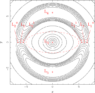
Figure 12: Contours of constant effective potential. The model is the same as in Fig. 1, except that we have added two small Kuz’min/Toomre discs centred on the positions of the $L_{1}$ and $L_{2}$ (see text). The total mass of each of these discs is $M_{a}$=0.025$M_{b}$ and their scale length is $r_{a}$ = 0.6. All Lagrangian points are marked by asterisks. Note that there are now nine Lagrangian points. The $L_{1}$ and $L_{2}$ are now minima of the effective potential and each one has on either side of it two more Lagrangian points. These are called $L^{i}_{1}$ (or $L^{i}_{2}$) and $L^{o}_{1}$ (or $L^{o}_{2}$), for the inner and outer one, respectively, and are saddle points.

In order for the theory as described so far to be applicable to barred spirals, their Lagrangian points $L_{1}$ and $L_{2}$ must be unstable. We will hereafter refer to this case as the standard case. If this were not the case, i.e. if the $L_{1}$ and $L_{2}$ became somehow stable, the Lyapunov orbits would also be stable even very near the $L_{1}$ and $L_{2}$ and thus the invariant manifolds described in Sect. 2.3 would not form. We thus want to test in this section whether the $L_{1}$ and $L_{2}$ are always unstable, or whether they could become stable, and, if so, under what conditions.

One way of achieving this stability could be by adding a concentration of matter around the $L_{1}$ and $L_{2}$. We tested this by adding two identical, small Kuz’min/Toomre discs (Kuz’min, 1956; Toomre, 1963), one centred on each of the $L_{1}$ and $L_{2}$. As can be seen in Fig. 12, this changes the topology of the iso-effective-potential curves. The $L_{1}$ and $L_{2}$, instead of being saddle points as in the standard case (Fig. 1), become minima. On either side of them two more equilibrium points form, one at larger and the other at smaller radii, which we call $L^{i}_{j}$ and $L^{o}_{j}$ ($j=1,2$), respectively for the inner and outer one. These are saddle points, so we can expect them to influence the dynamics in a way similar to that of the unstable $L_{1}$ ($L_{2}$) in the standard case.

Where could such an extra mass around the Lagrangian points come from? As we saw in Sect. 2.2, any orbit in the immediate vicinity of a Lyapunov orbit will not leave it immediately, but will first circle around it a couple or a few times before following the direction of the manifold. This would result in a mass concentration around $L_{1}$ ($L_{2}$) which would contribute to the necessary mass concentration. Furthermore, mass in this region could be contributed by specific morphological characteristics of the bar, such as star formation near the ends of the bar, or ansae (Sandage, 1961; Athanassoula, 1984; Martinez-Valpuesta, Knapen & Buta, 2007). This issue will be further discussed in Paper IV.

Figure 13: Stability diagram for the models discussed in Sect. 5. The solid line separates the region within which the $L_{1}$ and $L_{2}$ are stable from the region in which they are unstable; the stable being in the upper left part. $F$ is a measure of the mass of the Kuz’min/Toomre disc stabilising the $L_{1}$, or $L_{2}$ (see text) and $r_{a}$ is its scale length.

We studied the stability of the $L_{1}$ and $L_{2}$ using the method described in Appendix B and in Sect. 3 of Paper I. Two quantities influence this stability, namely the mass and the scale length of the two Kuz’min/Toomre discs, assumed to be identical. Since normalised quantities are more intuitive, instead of the mass we use the quantity $F=M_{KT}(r<r_{a})/M_{b}(r<r_{a})$, where $r_{a}$ is the scale length of the Kuz’min/Toomre disc, $M_{KT}(r<r_{a})$ is its mass within a distance equal to $r_{a}$ from its centre and $M_{b}(r<r_{a})$ is the mass of the bar within the same distance from the galaxy centre. The results of this stability analysis are shown in Fig. 13. The solid line separates the stable from the unstable region; the stable one being in the upper left part. As expected, stability is achieved when the Kuz’min/Toomre discs superposed on the $L_{1}$ and $L_{2}$ are sufficiently massive and sufficiently concentrated, in which case the $L_{1}$ and $L_{2}$ will become stable.

How are the dynamics in the vicinity of $L_{1}$ ($L_{2}$) modified in cases where these Lagrangian points are stable? We will first describe in some detail a case whose corresponding standard model has an $rR_{1}$ morphology. The Lagrangian points $L_{j}$, $L^{i}_{j}$ and $L^{o}_{j}$ ($j=1,2$) are surrounded each by a family of periodic orbits. Examples of the periodic orbits are given with full black lines in Figs. 14 and  15. The orbits in all three families are oriented perpendicular to the direction of the bar major axis, and have shapes similar to those of the Lyapunov orbits in the standard case. For a given energy, the orbit around $L_{1}$ ($L_{2}$) has the largest extent, followed by that around $L^{i}_{1}$ ($L^{i}_{2}$). The orbit around $L^{o}_{1}$ ($L^{o}_{2}$) has the smallest extent. The orbit around $L_{1}$ ($L_{2}$) is stable while the other two are unstable, as the Lyapunov orbits in the standard case.

How do the invariant manifolds look in a case with six Lagrangian points along the direction of the bar major axis? Figs. 14 and 15 show the unstable and stable manifolds, respectively, in the immediate neighbourhood of $L_{1}$. The model used in this example is our fiducial model A (Sect. 2.1) with two extra Kuz’min/Toomre discs of total mass equal to 0.025$M_{b}$ each and a scale length $r_{a}$=0.6. The unstable and the stable manifolds associated with $L_{1}^{o}$ have two branches each, one ingoing and one outgoing, as is the case for the manifolds emanating from $L_{1}$ in the standard case where $L_{1}$ is unstable (Paper I and Sect. 2.3). The inwards unstable branch has a very interesting morphology. Emanating from $L_{1}^{o}$, it circumvents $L_{1}$ from the positive $y$ values and reaches the immediate neighbourhood of $L_{1}^{i}$ before heading towards the outer parts of the bar (upper right panel in Fig. 14). The morphology of the outgoing branch of the stable manifold of the $L_{1}^{o}$ is also very interesting (upper right panel in Fig. 15). Material moves from the bar region to the vicinity of the $L_{1}^{i}$, then circumvents $L_{1}$ from negative values of $y$ to join finally the vicinity of $L_{1}^{o}$.

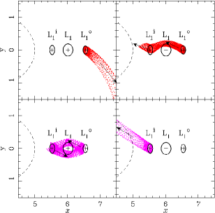
Figure 14: Unstable manifolds for a case with a stable $L_{1}$ Lagrangian point. The model is the same as for Fig. 12. On either side of the $L_{1}$ we note the inner and outer unstable Lagrangian points, $L_{1}^{i}$ and $L_{1}^{o}$, respectively, each surrounded by a periodic orbit. The unstable manifolds for the same energy are also plotted (red). The upper (lower) panels show the unstable manifolds of the outer (inner) Lagrangian point, $L^{o}_{1}$ ($L^{i}_{1}$). The arrows show the direction of the motion within the manifolds and the dashed line gives the outline of the bar.

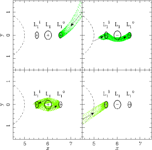
Figure 15: Same as Fig. 14, but for the stable manifolds (green).

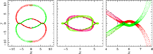
Figure 16: Full outline of the manifolds (left panel), their inner part (middle panel) and the region around the Lagrangian point (right panel) for the model whose equipotentials are shown in Fig. 12. Unstable manifolds are plotted in red and stable ones in green. The dashed black line shows the bar outline and the full black lines give the periodic orbits of the same energy as the manifold, one around $L_{1}^{i}$ and one around $L_{1}^{o}$.

The manifolds of the $L_{1}^{i}$ are even more elaborate. As for $L_{1}^{o}$, the unstable and the stable manifolds associated with $L_{1}^{i}$ have two branches each. For the unstable manifold, one of the branches takes material from the vicinity of $L_{1}^{i}$ and pushes it towards the outer parts of the bar, i.e. has a very simple morphology (lower right panel in Fig. 14) . On the contrary, the second unstable branch has a very complicated morphology. Material from the vicinity of the $L_{1}^{i}$ moves outwards, circumventing $L_{1}$ from the negative values of $y$ to reach the vicinity of $L_{1}^{o}$. Before reaching it, however, it turns around, circumvents $L_{1}$, now from the positive values of $y$, and thus returns to the vicinity of $L_{1}^{i}$ (bottom left panel of Fig. 14). The branches of the stable manifolds have a similar morphology (bottom panels of Fig. 15). Note also that the innermost branches of the manifolds (both stable and unstable) of $L_{1}^{i}$, as well as the outermost branches of $L_{1}^{o}$ (both stable and unstable) have most of their motion along the manifold, as was the case for the strongly unstable Lagrangian points of the standard case (see Sect. 4 and Fig. 9). On the contrary, the branches between $L_{1}^{i}$ and $L_{1}^{o}$ are much more densely packed, with a considerable part of the motion perpendicular to the manifold loci.

We repeated these calculations, now for a case whose corresponding standard model (i.e. the model without the two extra Kuz’min/Toomre discs) has a spiral structure. The dynamics in the vicinity of the $L_{1}^{i}$, $L_{1}$ and $L_{1}^{o}$ are very similar, so we do not reproduce the corresponding plots here. There are, nevertheless, a number of differences. One is that now the Lyapunov orbit is elongated along the direction of the bar major axis, i.e. perpendicular to the direction of the example shown in Figs. 14 and 15. Further investigation is necessary to explain this change of orientation. A second difference is that the morphology of the unstable inner branch of $L_{1}^{o}$ and that of the unstable outer branch of $L_{1}^{i}$ are reversed. Thus the former encircles $L_{1}$ and returns to $L_{1}^{o}$, while the latter proceeds outwards from the bar. The dynamics of this region needs further investigation, but we will here be interested only in the global morphology of the manifolds in these non-standard cases.

The left panel of Fig. 16 displays the full outline of the manifolds for the example where the standard case (i.e. the case without the two extra Kuz’min/Toomre discs) is $rR_{1}$ and shows a very interesting point. Namely the global morphology is of $rR_{1}$ type, the same as of the corresponding standard case. The loci of the branches, both stable and unstable, of the $L^{o}_{1}$ and $L^{i}_{1}$ in and around the bar region nearly superpose. A similar statement can be made for the outer branches, i.e. the ones beyond the Lagrangian points. They, therefore, reinforce each other. This leads to the $rR_{1}$ morphology, i.e. the manifold loci form an inner ring elongated along the bar and an outer one, elongated perpendicular to it, provided the distance between the $L_{1}^{i}$ and $L_{1}^{o}$ is not too large, i.e. in cases where the ‘island’ of stability around the $L_{1}$ ($L_{2}$) is of small extent. Thus the global morphology was not changed by the stabilisation of the $L_{1}$ and $L_{2}$.

The middle panel of Fig. 16 shows the inner parts of the manifold clearer. We used the same model, except that we have now integrated over longer times. Several interesting comparisons to bar morphologies can be now made. First, part of the outline is rectangular-like. A second point is that the outermost parts of this structure protrude from either part of the bar along the direction of the bar major axis. These two features need to be stressed here, because they will be used in Paper IV to describe specific morphological features of observed bars.

Similarly, the model which had a spiral morphology before the two Kuz’min/Toomre discs are added to the bar ends still keeps that morphology after they are added and the $L_{1}$ and $L_{2}$ stabilised. This brings us to the interesting conclusion that the global morphology does not change wildly, as long as the stability islands are not too extended. Nevertheless, there are some changes, notably in the ring diameter sizes. This will be further discussed in Paper IV, when we compare the ratio of observed rings with the corresponding quantities for manifolds.

6 The behaviour of gas

A number of simulations have shown the formation of spirals and rings from gas (e.g. Schwarz, 1981, 1984, 1985; Combes & Gerin, 1985). We should thus compare the dynamics of gas with that of the manifolds presented here. Gas, however, has different equations of motion from stars, so we need to modify our calculations accordingly. Schwarz (1979, 1981, 1984, 1985) uses sticky particles to simulate the gas and models collisions in a particularly straightforward way, so we can introduce a similar procedure also in our calculations. In Schwarz’s simulations, particles represent gaseous clouds which lose a certain fraction of their kinetic energy when they collide. In practise, they lose a certain fraction $f$ of their velocity (Schwarz, 1981), or only of one component of their velocity (Schwarz, 1984, 1985), i.e. of the component of velocity that is along the line joining the two particles. Thus, after the collision this component is $v_{2}=-(1-f)v_{1}$, where the subscripts 1 and 2 designate the times before and after the collision, respectively. The values of $f$ in Schwarz’s simulations range between 0.8 and 1. We introduced a similar process in our calculations in the following way. We calculated a number of orbits of the outer branch of the unstable manifold and drew random numbers to find where along its trajectory each particle will undergo a collision. We tried different numbers of collisions per half bar rotation, around the values used by Schwarz. To determine the result of a collision, we take a small box around the collision position and calculate the average velocity of all orbits in that box. We then decrease the relative velocity of the particle parallel to this mean (i. e. we decrease one velocity component) by a factor $-(1-f)$. We ran a number of such simulations and show an example in Fig. 17. For this, we used the potential of Schwarz’s standard model for the values of the free parameters $a$ = 2.6, $q$ = 0.1 and $\Omega_{p}$ = 0.27, for which he gives sufficient results and information in his papers to allow comparisons. This potential gives manifolds with $rR_{1}$ morphology. The outer branch is plotted in black in Fig. 17, together with the positions of the gaseous particles (in red). To allow a comparison, we only include gaseous particles that have energies above that of $L_{1}$. For this example we used $f$ = 0.8, which leads to a mean energy dissipation per particle of 6.2 $\times 10^{-4}$, in good agreement with the numbers given by Schwarz (1981). Other numerical values give qualitatively similar results. Fig. 17 shows that there is in general good agreement between the loci of the gaseous and of the stellar arm. Furthermore, the gaseous arm is somewhat more concentrated than the stellar arm, more so for a larger number of collisions per revolution. In the particular case of Fig. 17 we used three collisions per half revolution.

Qualitatively, the above results can be understood as follows. Sticky particles (i.e. gaseous particles) follow the same orbits as the stellar ones, except for the collisions. This ensures a general similarity. Due to the collisions, the gaseous particles lose part of their kinetic energy and their velocity approaches that of the mean. In Paper I, we compared the loci of manifolds for different energies and found that the ones with the smaller energies lie in configuration space within the ones with the higher energies. This means that the corresponding spiral arms, or rings will be thinner for the lower energies. Thus, when the particles lose energy they will fall onto an orbit nearer to the mean and the arms, or rings will become thinner. This is exactly what is found with the calculations leading to Fig. 17. Thus, roughly speaking, one can think of the lowest energy manifolds (i.e. the ones having the energy of $L_{1}$ and $L_{2}$) as an attractor, to which the gaseous trajectories will tend to because of the dissipation due to the collisions.

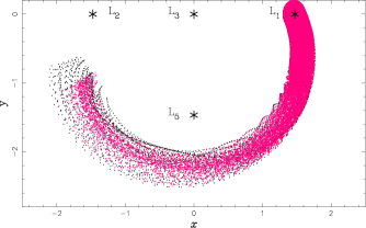
Figure 17: Comparison of the spiral arm loci as calculated with (red) and without (black) collisions. See text for a description of the calculations.

7 Summary

Since the early work of B. Lindblad (1963), density waves have been commonly assumed to be at the basis of any explanation of spiral structure formation. Here we present an alternative viewpoint, applicable specifically to barred galaxies. This explains the formation of spiral arms, as well as of inner and outer rings, in a common theoretical framework. We presented this in Papers I and II and elaborate it further here. According to our theory, it is the unstable Lagrangian points located at the ends of the bar and the corresponding manifolds that are responsible for the formation of spirals and rings. These manifolds drive orbits, which are in fact chaotic but are confined by the manifolds, so that they create over-densities which have the right shape to explain the spirals and the rings.

In Paper II we noted that different morphologies are possible, but did not try and understand which bar properties were responsible for them. This was one of our objectives here and to achieve it we used three different types of bar models. In particular, we showed that the bar strength has a considerable effect on the properties of the manifolds. Strong bars have more unstable $L_{1}$ and $L_{2}$ Lagrangian points than weak bars. Material in their manifolds needs less time to perform half a revolution around the galactic centre. The difference can be considerable; factors of 5, or even higher, are possible. In the weaker bar cases, the manifolds stay near the zero velocity curves of the same energy, while they depart considerably from them if the bar forcing in the relevant radial range is very strong. This brings about different morphologies. If the non-axisymmetric forcing at and somewhat beyond $r=r_{L_{1}}$ is relatively weak, the outer branches of the manifolds have the shape of $R_{1}$ rings or pseudorings. Spirals, as well as $R_{2}$ and $R_{1}R_{2}$ rings and pseudorings, are formed by stronger bars.

The circulation of material within the manifolds is also different. In the relatively weak bar cases, which form $rR_{1}$ morphologies, the mass elements move either within the inner branches, or within the outer branches, or from the inner branches to the outer ones and then back to inner ones again. In this third case, material is moving from the region within corotation to the region outside it and vice versa via the neighbourhood of the $L_{1}$ and $L_{2}$. Averaged over a sufficiently long time, this amounts to circulation of material within a given thick annulus, but no net motion of material inwards or outwards. This is not true for the cases where the non-axisymmetric forcing beyond corotation is stronger and which have a spiral morphology. In such cases, material moves from the region within corotation to the region outside it, but does not return. So, in total, this brings a net movement of material from within corotation outwards, to the outermost parts of the disc and may contribute to the radial extension of the disc.

We found also that, if there is sufficient mass concentration around the $L_{1}$ and $L_{2}$, these Lagrangian points will be stable. On either side of each one of them and still on the direction of the bar major axis, there will be another unstable Lagrangian point, so that there will be nine Lagrangian points in total, four unstable and five stable. Two of the stable ones are in the direction of the bar minor axis and are the $L_{4}$ and the $L_{5}$, as in the standard case. The third stable one is located at the centre of the coordinates. The remaining two stable ones and the four unstable ones are in the direction of the bar major axis. This setting creates very interesting circulation patterns around the $L_{1}$ and $L_{2}$, but leaves the global morphology unchanged. For the case of a relatively weak bar, we still have an $rR_{1}$ morphology, but the inner and outer rings will not necessarily touch each other. For the case of a strong bar which had a spiral morphology before the mass concentrations around the $L_{1}$ and $L_{2}$ were introduced, we still find spiral structure after the mass concentrations are introduced.

We also introduced collisions and dissipation to the manifold calculations, in order to roughly model the gas properties. We found that this does not influence the existence of the spiral arms or rings and not much their shape and winding. The amount of dissipation, however, does influence the width of the arms. These become thinner as the dissipation is increased, so that the gaseous arm comes nearer to the lowest energy manifold.

The next step after presenting a theory is to check whether it is applicable to the rings and spirals observed in disc galaxies. This will be the subject of an accompanying paper, where we will also make a global discussion on the results of the two papers together.

Appendix A Models

Our basic barred galaxy model in this paper will be the one introduced by Athanassoula (1992a). Its axisymmetric component consists of the superposition of a disc and a spheroid, whose basic parameters are determined so that the rotation curve of the galactic model has the desired characteristics. The disc is modelled as a Kuz’min/Toomre disc (Kuz’min, 1956; Toomre, 1963) of surface density

$$\sigma(r)=\frac{V_{d}^{2}}{2\pi r_{d}}\left(1+\frac{r^{2}}{r_{d}^{2}}\right)^{-3/2}.$$ (2)

The parameters $V_{d}$ and $r_{d}$ set the scales of the velocities and radii, respectively. The spheroid is modelled using a density distribution of the form

$$\rho(r)=\rho_{s}\left(1+\frac{r^{2}}{r_{s}^{2}}\right)^{-3/2},$$ (3)

where $\rho_{s}$ and $r_{s}$ determine its central density and scale length. Spheroids with high concentration have high values of $\rho_{s}$ and small values of $r_{s}$, the opposite being true for spheroids of low concentration. Although we include two separate axisymmetric components, it is important to note that, in fact, what matters in this study is only the total axisymmetric rotation curve and not its decomposition into components.

The bar component is described by a Ferrers ellipsoid (Ferrers, 1877), whose density distribution is described by the expression:

$$\rho=\left\{\begin{array}[]{lr}\rho_{0}(1-m^{2})^{n}&m\leq 1\\ 0&m\geq 1,\end{array}\right.$$ (4)

where $m^{2}=x^{2}/a^{2}+y^{2}/b^{2}$. The values of $a$ and $b$ determine the shape of the bar, $a$ being the length of the semi-major axis, which, in the rotating frame of reference, is placed along the $x$ coordinate axis, and $b$ being the length of the semi-minor axis. The parameter $n$ measures the degree of concentration of the bar. High values of $n$ correspond to a high concentration, while a value of $n=0$ is the extreme case of a constant density bar. The parameter $\rho_{0}$ represents the central density of the bar. For these models, the quadrupole moment of the bar is given by the expression

$$Q_{m}=M_{b}(a^{2}-b^{2})/(5+2n),$$

where $M_{b}$ is the mass of the bar, equal to

$$M_{b}=2^{(2n+3)}\pi ab^{2}\rho_{0}\Gamma(n+1)\Gamma(n+2)/\Gamma(2n+4)$$

and $\Gamma$ is the gamma function.

All models with these mass components will be generically referred to in this paper as model A. They have essentially four free parameters which determine the dynamics in the bar region. The axial ratio $a/b$ and the quadrupole moment (or mass) of the bar $Q_{m}$ (or $M_{b}$), will determine the strength of the bar. The third parameter is the angular velocity, or pattern speed, determined by the Lagrangian radius $r_{L}$. The last free parameter is the central density of the model $\rho_{c}=\rho_{s}+\rho_{0}$. For reasons of continuity we will use the same numerical values for the model parameters as in Athanassoula (1992a). The axisymmetric component is fixed by setting a maximum disc circular velocity of 164.204 km / sec at $r$=20 kpc, and $r_{s}$ is determined by fixing the total mass of the spheroid and bar components within $r$ = 10 kpc to $4.87333\times 10^{4}~{}M_{\odot}$ , while fixing the combined central density of the bar and bulge to $\rho_{c}$. More information on these models can be found in Athanassoula (1992a).

The Ferrers bars are realistic models of bars and have been widely used so far in orbital structure studies within and in the immediate neighbourhood of bars (e.g. deVaucouleurs & Freeman, 1972; Athanassoula et al. , 1983; Papayannopoulos & Petrou, 1983; Pfenniger, 1984; Athanassoula, 1992a, b; Skokos et al. , 2002a, b). They contain parameters with physical meaning, such as the bar mass or axial ratio, that can be obtained from, or compared to, observations. They have, however, one disadvantage, namely that in models using such bars the non-axisymmetric component of the force decreases very abruptly beyond a certain radius so that the axisymmetric component dominates in the outer regions. This is of no importance if one is interested in the orbital structure or the gas flow in the bar region, as the studies mentioned above, but in studies like the present one, where one is interested in the region outside the bar, this may introduce a bias, since models with high non-axisymmetric forces beyond corotation will not be included.

In order to remedy this, we use here two further models, also often used in the literature, which have an ad hoc bar potential, i.e. a potential that is not associated to a particular density distribution. Ad hoc models have some disadvantages. They are simple mathematical expressions for the potential and do not originate from a realistic density distribution. This means that the corresponding density distribution may have some undesired features, e.g. for very strong non-axisymmetric perturbations the total density could even be negative locally. Furthermore, they do not contain simple parameters that can be directly and straightforwardly associated to observable quantities, like the bar length, mass, or axial ratio. Most of them are of the form $\epsilon A(r)\cos(2\theta)$, i.e. contain no $\cos(m\theta)$ terms with $m>2$. This means that the parameter $\epsilon$ is associated with the mass of the bar and that there is no parameter to regulate its axial ratio. Despite all these shortcomings, ad hoc potentials have been widely used because they have the important advantage of being adaptable to the problem at hand. I.e., with a proper choice of the $A(r)$ function one can obtain a potential with the desired properties, for example, in our case, a potential with an important $m=2$ contribution between corotation and outer Lindblad resonance.

The first ad hoc bar potential we use is adapted from Dehnen (2000) and has the form

$$\Phi(r,\theta)=-\frac{1}{2}\epsilon v_{0}^{2}\cos(2\theta)\left\{{\begin{array}[]{ll}\displaystyle 2-\left(r/\alpha\right)^{n},&r\leq\alpha\rule[-14.22636pt]{0.0pt}{28.45274pt}\\ \displaystyle\left(\alpha/r\right)^{n},&r\geq\alpha.\rule[-14.22636pt]{0.0pt}{28.45274pt}\end{array}}\right.$$ (5)

The parameter $\alpha$ is a characteristic length scale of the bar potential and $v_{0}$ is a circular velocity. The parameter $\epsilon$ is a free parameter related to the bar strength. In this paper we use $\alpha$ = 5 and $n~{}=~{}0.75$. For this model we will use the same axisymmetric component as for model A and we will refer to it as model D.

Our third model has the bar potential :

$$\Phi(r,\theta)=\hat{\epsilon}\sqrt{r}(r_{1}-r)\cos(2\theta),$$ (6)

where $r_{1}$ is a characteristic scale length of the bar potential, which we will take for the present purposes to be equal to 20 kpc. The parameter $\hat{\epsilon}$ is related to the bar strength. This type of model has already been widely used in studies of bar dynamics (e.g. Barbanis & Woltjer, 1967; Contopoulos & Papayannopoulos, 1980; Contopoulos, 1981). We will couple this bar with the axisymmetric part used in model A and we will refer to it as the BW model.

Throughout this paper we use the following system of units: For the mass unit we take a value of $10^{6}M_{\odot}$, for the length unit a value of 1 kpc and for the velocity unit a value of 1 km/sec. Using these values, the unit of the Jacobi constant will be 1 km²/sec².

Appendix B Linear stability analysis

In this appendix we will briefly present a linear solution to the stability of the Lagrangian points. Setting $x_{1}=x,\quad x_{2}=y,\quad x_{3}=\dot{x}$ and $\quad x_{4}=\dot{y}$, the equations of motion are schematically written as a system of first order differential equations,

$$\dot{x_{i}}=f_{i}(x_{1},\dots,x_{4})~{}~{}~{}~{}~{}~{}~{}~{}~{}i=1,\dots,4\\$$ (7)

In the neighbourhood of the $L_{1}$ (or equivalently $L_{2}$) Lagrangian points these can be written as

$$\left\{\begin{array}[]{rclcl}\dot{x_{1}}&=&f_{1}(x_{1},\dots,x_{4})&=&x_{3}\\ \dot{x_{2}}&=&f_{2}(x_{1},\dots,x_{4})&=&x_{4}\\ \dot{x_{3}}&=&f_{3}(x_{1},\dots,x_{4})&=&2\Omega_{p}\,x_{4}-\Phi_{xx}x_{1}\\ \dot{x_{4}}&=&f_{4}(x_{1},\dots,x_{4})&=&-2\Omega_{p}\,x_{3}-\Phi_{yy}x_{2}.\\ \end{array}\right.$$ (8)

The differential matrix associated to this system is

$$Df_{x}(L_{1})=\left(\begin{array}[]{cccccc}0&0&1&0\\ 0&0&0&1\\ -\Phi_{xx}&0&0&2\Omega_{p}\\ 0&-\Phi_{yy}&-2\Omega_{p}&0\\ \end{array}\right).$$

We obtain the stability character of $L_{1}$ by studying the eigenvalues of this matrix. It has four eigenvalues: $\lambda$, $-\lambda$, $\omega i$ and $-\omega i$, where $\lambda$ and $\omega$ are positive values and the equations of motion can be written as

$$\left\{\begin{array}[]{l}x(t)=X_{1}e^{\lambda t}+X_{2}e^{-\lambda t}+X_{3}\cos(\omega t+\phi),\\ y(t)=X_{4}e^{\lambda t}+X_{5}e^{-\lambda t}+X_{6}\sin(\omega t+\phi).\\ \end{array}\right.$$ (9)

If $\lambda$ is a real number, $L_{1}$ is a linearly unstable point. Larger values of $\lambda$ denote more unstable systems.

References

- Athanassoula (1980) Athanassoula, E. 1980, A& A, 88, 184
- Athanassoula (1984) Athanassoula, E. 1984, Phys. Rep., 114, 319
- Athanassoula (1992a) Athanassoula, E. 1992a, MNRAS, 259, 328
- Athanassoula (1992b) Athanassoula, E. 1992b, MNRAS, 259, 345
- Athanassoula (2005) Athanassoula, E. 2005, MNRAS, 358, 1477
- Athanassoula et al. (1983) Athanassoula, E., Bienaymé, O., Martinet, L., Pfenniger, D. 1983, A& A, 127, 349
- Barbanis & Woltjer (1967) Barbanis, B., Woltjer, L. 1967, ApJ, 150, 461
- Binney (1981) Binney, J. 1981, MNRAS, 196, 455
- Binney & Tremaine (2008) Binney, J., Tremaine, S. 2008, Galactic Dynamics, Second Edition, Princeton Univ. Press, Princeton
- Buta (1995) Buta, R. 1995, ApJS, 96, 39
- Combes & Gerin (1985) Combes, F., Gerin, M. 1985, A&A, 150, 327
- Contopoulos (1981) Contopoulos, G. 1981, A& A, 102, 265
- Contopoulos (2002) Contopoulos, G. 2002, Order and Chaos in Dynamical Astronomy, Springer Verlag, Berlin
- Contopoulos & Papayannopoulos (1980) Contopoulos, G., Papayannopoulos, T. 1980, A& A, 92, 33
- deVaucouleurs & Freeman (1972) de Vaucouleurs, G., Freeman, K. C. 1972, Vistas in Astronomy, 14, 163
- Dehnen (2000) Dehnen, W., 2000, AJ, 119, 800
- Danby (1965) Danby, J. M. A. 1965, AJ, 70, 501
- Elmegreen & Elmegreen (1989) Elmegreen, B.G., Elmegreen, D.M. 1989, ApJ, 342, 677
- Feldman & Lin (1973) Feldman, S. I., Lin, C. C. 1973, Stud. Appl. Math., 52, 1
- Ferrers (1877) Ferrers N. M. 1877, Q.J. Pure Appl. Math., 14, 1
- Gómez et al. (2004) Gómez, G., Koon, W.S., Lo, M. W., Marsden, J. E., Masdemont, J. J., Ross, S. D. 2004, Nonlinearity, 17, 1571
- Kaufmann & Contopoulos (1996) Kaufmann, D.E., Contopoulos, G. 1996, A&A, 309, 381
- Koon et al. (2000) Koon, W. S. Lo, M. W., Marsden. J. E., Ross, S. D. 2000, Chaos, 10, 2, 427
- Kuz’min (1956) Kuz’min, G. 1956, Astron. Zh., 33,27
- Lindblad (1963) Lindblad, B. 1963, Stockholms Observatorium Ann., Vol. 22, No. 5
- Lindblad, Lindblad & Athanassoula (1996) Lindblad, P. A. B., Lindblad, P. O. & Athanassoula, E. 1996, A&A, 313, 65
- Lyapunov (1949) Lyapunov, A. 1949, Ann. Math. Studies, 17
- Martinez-Valpuesta, Knapen & Buta (2007) Martinez-Valpuesta, I.; Knapen, J. H.; Buta, R. 2007, AJ, 134, 1863
- Papayannopoulos & Petrou (1983) Papayannopoulos, T., Petrou, M. 1983, A& A, 119, 21
- Patsis (2006) Patsis, P.A., 2006, MNRAS, 369, L56
- Patsis et al. (2002) Patsis, P., Skokos, Ch., Athanassoula, E. 2002, MNRAS, 337, 578
- Pfenniger (1984) Pfenniger, D. 1984, A& A, 134, 373
- Quillen, Frögel & Gonzalez (1994) Quillen, A. C., Frögel, J., Gonzalez, R. 1994, ApJ, 437, 162
- Romero-Gómez et al. (2006) Romero-Gómez, M., Masdemont, J.J., Athanassoula, E., García-Gómez, C. 2006, A& A, 453, 39 (Paper I)
- Romero-Gómez et al. (2007) Romero-Gómez, M., Athanassoula, E., Masdemont, J.J., García-Gómez, C. 2007, A& A, 472, 63 (Paper II)
- Romero-Gómez et al. (2008) Romero-Gómez, M., Masdemont, J.J., García-Gómez, C., Athanassoula, E. 2008, Communications in Nonlinear Science and Numerical Simulations, DOI: 10.1016/j.cnsns.2008.07.013
- Sandage (1961) Sandage, A. 1961, The Hubble Atlas of Galaxies (Washington: Carnegie Institution)
- Schwarz (1979) Schwarz, M.P. Ph.D. Thesis, Australian National University (1979)
- Schwarz (1981) Schwarz, M.P. 1981, ApJ, 247, 77
- Schwarz (1984) Schwarz, M.P. 1984, MNRAS, 209, 93
- Schwarz (1985) Schwarz, M.P. 1985, MNRAS, 212, 677
- Skokos et al. (2002a) Skokos, Ch., Patsis, P.A., Athanassoula, E. 2002a, MNRAS, 333, 847
- Skokos et al. (2002b) Skokos, Ch., Patsis, P.A., Athanassoula, E. 2002b, MNRAS, 333, 861
- Toomre (1963) Toomre, A. 1963, ApJS, 138, 385
- Voglis, Stavropoulos & Kalapotharakos (2006) Voglis, N., Stavropoulos, I., Kalapotharakos, C. 2006a, MNRAS, 372, 901
- Voglis, Tsoutsis & Efthymiopoulos (2006) Voglis, N., Tsoutsis, P., Efthymiopoulos, C. 2006b, MNRAS, 373, 280