Stellar mass estimates in early-type galaxies: procedures, uncertainties and models dependence

Abstract

The aim of the present paper is to quantify the dependence of the estimates of luminosities and stellar mass content of early-type galaxies on the different models and model parameters which can be used to analyze the observational data. The paper is organized in two parts. The first one analyzes the dependence of the $\mathcal{M/L}$ ratios and of the k-corrections in different bands on model parameters (Initial Mass Function, metallicity, star formation history, age), assuming some among the most popular spectrophotometric codes usually adopted to study the evolutionary status of galaxies: Bruzual & Charlot (2003, BC03), Charlot & Bruzual (2008, CB08), Maraston (2005, Ma05), Fioc & Rocca-Volmerange (1997, PEGASE), Silva et al. (1998, GRASIL). The second part of our work is dedicated to quantify the reliability and systematics affecting the mass and luminosity estimates obtained by means of the best fitting technique applied to the photometric SEDs of early-type galaxies at $1<z<2$. To this end, we apply the best fitting technique to some mock catalogs built on the basis of a wide set of models of early-type galaxies. We then compare the luminosity and the stellar mass estimated from the SED fitting with the true known input values. The goodness of the mass estimate is found to be dependent on the mass estimator adopted to derive it, but masses cannot anyhow be retrieved better than within a factor 2-3, depending on the quality of the available photometric data and/or on the distance of the galaxies since more distant galaxies are fainter on average and thus affected by larger photometric errors.

Finally, we present a new empirical mass estimator based on the K band apparent magnitude and on the observed (V-K) colour. We show that the reliability of the stellar mass content derived with this new estimator for early-type galaxies and its stability are even higher than those achievable with the best classic estimators, with the not negligible advantage that it does not need any multi-wavelength data fitting.

1 Introduction

The formation and evolution history of the early-type galaxies represent a key ingredient in the more global models of galaxy formation. Early-type galaxies are elliptical and bulge dominated galaxies which contain most of the present stellar mass and which include the most massive galaxies of the local Universe. They are characterized by a pronounced 4000 Å break, corresponding to rest frame red UV-optical colours. This feature is typical of evolved stellar populations (i.e. old with respect to the age of the Universe at the redshift of the galaxy) with almost absent star forming activity.

Two approaches can be pursued in the study of the past history of this class of objects: the archaeological approach, that studies in details local samples of galaxies attempting to derive their past history, or the direct analysis of samples of galaxies at different redshift (i.e. at different stages of their evolution). In both the two cases, the spectrophotometric models allow the interpretation of the observed spectral properties of galaxies and thus they are a basic ingredient to correctly derive their formation and evolution history.

One of the fundamental parameters used to derive the past history of the early-type galaxies is their stellar mass content. Indeed, the measure of the stellar mass of early-type galaxies is involved in some useful scale relations such as the size-mass relation by Shen et al. (2003). Furthermore, the origin and/or evolution of the early-type galaxies seem to follow different ways or at least different time scale as a function of their stellar mass, the so-called downsizing (e.g., Bell et al. 2005; Thomas et al. 2005). Thus, in the last years it has become important to assess the stellar mass content of early-type galaxies in various range of redshift.

The stellar mass content of galaxies is usually derived from luminosity measures by means of conversion factors supplied by models which for a given set of physical parameters well describe their observed Spectral Energy Distribution (SED). The degeneracy among the model parameters which allow to reproduce the observed SEDs of the galaxies (e.g. age, metallicity and star formation history) and the differences in the conversion factors supplied by different models determine the uncertainty of the mass estimates. The aim of the present paper is to study the dependence of the estimates of the stellar mass content and of luminosity of the early-type galaxies on the choices of different available models and of different parameters defining the models. A forthcoming paper will focus on the problem of the age determination.

The paper is organized in two parts. The first one (§2 to §3) analyzes the dependence of the $\mathcal{M/L}$ ratios and of the k-corrections in different bands on model parameters (Initial Mass Function, metallicity, star formation history, age), assuming some among the most popular spectrophotometric codes usually adopted to study the evolutionary status of galaxies: Bruzual & Charlot (2003, BC03), Charlot & Bruzual (2008, CB08), Maraston (2005, Ma05), Fioc & Rocca-Volmerange (1997, PEGASE), Silva et al. (1998, GRASIL). In particular, §2 introduces and defines the main parameters which can be varied in the spectrophotometric models adopted to reproduce the spectral properties of the early-type galaxies, and it presents the main features of the models which will be used in the following sections, picking out the basic differences among them. §3 presents the results which can be obtained when different spectrophotometric codes are used to derive k-corrections and $\mathcal{M/L}$ ratios needed to transform the apparent magnitudes into mass estimates. In the last part of this section, it is presented a self consistent relation that allows to easily calculate $\mathcal{M}$ from the apparent K band magnitude as a function of z that is valid for all the models here considered within 0.15 dex (a factor 1.4).

The second part of the paper (§4) is dedicated to quantify the reliability and systematics which can result in the mass and luminosity estimates obtained by means of the best fitting technique applied to the photometric SEDs of early-type galaxies at $1<z<2$. A wide range of simulated spectra are used to build mock photometric catalogs. The measures of the luminosities and of the stellar masses of the simulated galaxies are compared with the true known input values. Appendix A complements this comparison as far as the $\mathcal{M/L}$ ratios are concerned. In the end of this section, we present a test aimed at verifying how different are the stellar mass estimates obtained with different set of templates created with different codes (§4.3).

Before concluding the paper, §5 presents a new mass estimator based on the apparent K band magnitude and (V-K) colour. It is demonstrated that its reliability is similar to that of the best most commonly used mass estimators despite the simplicity of its calculation that does not need any multi-wavelength data fitting. §6 summarizes the basic results found in the present work.

2 The models

In this section, we introduce the main parameters which can be varied in the spectrophotometric models adopted to reproduce the spectral properties of the early-type galaxies. The main features of the models which will be compared in the following sections are also presented.

2.1 Parameters

The spectrophotometric models are codes which produce the expected Spectral Energy Distribution (SED) for a given set of parameters describing a stellar population. The basic parameters defining a stellar population are: 1) stellar metallicity $Z$; 2) Initial Mass Function (IMF); 3) stellar evolutionary tracks; 4) stellar spectral library; 5) star formation history (SFH) and formation redshift ($z_{f}$) of the stellar content. Stellar evolutionary tracks and the stellar spectral library are usually fixed or “suggested” by the spectrophotometric codes, and for those compared in this work they will be listed below in the next part of this section. As far as the other parameters are concerned (i.e. $Z$, IMF and SFH), they represent the main adjustable variables when reproducing galaxies spectra. In the following sections, we will present the different results which can be achieved under different assumptions for these 3 parameters.

Since this work is devoted to the analysis of the spectral data of early-type galaxies, few remarks on some restrictions on the variability of SFH and $z_{f}$ have to be done. Indeed, observations collected so far have outlined a picture in which the bulk of stars in the early-type galaxies (at least in the most massive among them, $\mathcal{M}$$>10^{11}$ $\mathcal{M}$_⊙) formed at $z>2$ and passively evolved down to the present epoch. For example, from the observations of local and nearby samples of early-type galaxies, it can be deduced that massive field early-type galaxies should have formed their stellar content around $z\sim 2$ over short (i.e. $\tau<1$ Gyr) star formation timescales (Thomas et al. 2005). Furthermore, the analysis of the Fundamental Plane of early-type galaxies at $z\sim 1$ in the field (di Serego Alighieri et al. 2005, van der Wel et al. 2005, Treu et al. 2005, van der Wel et al. 2004, van Dokkum et al. 2003) and in clusters (e.g. Bender et al. 1998) fully supports a scenario in which their stars formed at $z>2$ and only the less massive spheroids could have been involved in star forming episodes at $z<1.2$. Similar results come from the analysis of the Faber & Jackson Relation (FJR, Faber & Jackson 1976) of a sample of field early-type galaxies at $\sim 0.7$ (Ziegler et al. 2005). At higher redshift ($z>1$) confirmations of this picture are recently coming out. For example, McCarthy et al. (2004) found a median age of 1.2 Gyr in a sample of 20 evolved galaxies at $z\sim 1.5$, and Daddi et al. (2005) report ages of about 1 Gyr for 7 galaxies at $1.4<z<2.5$. Longhetti et al. (2005) from the analysis of a sample of 10 massive ($\mathcal{M}$$>10^{11}$ $\mathcal{M}$_⊙) early-type galaxies confirm that the formation of early-type galaxies is well described assuming $2<z_{f}<3.5-4$ and SF time scales shorter than 1 Gyr. Thus, we consider as SFHs good to reproduce the spectral properties of the early-type galaxies only those with SF time scale shorter than 1 Gyr. We will also assume in the following an indicative formation redshift of their stellar content $z_{f}=4$ that will be used to associate to each value of $z$ the corresponding age of their stellar populations equal to the time elapsed since their formation. Even in the possible case that the assembly history of early-type galaxies was driven by major mergers at $z<2$, the latter must be “dry” (i.e. dissipationless, Bell et al. 2006; van Dokkum 2005) and they should have small effects on their global total star formation histories. On the other hand, if multiple frequent minor mergers at $z<2$ contribute to grow the stellar mass of early-type galaxies, these should add only small percentages to their total stellar content (Bournaud, Jog & Combes 2007). In both cases, the simplified assumption of the exponentially declining star formation history with time scale shorter than 1 Gyr started at $z\sim 4$ remains a realistic description of the formation and evolution history of the early-type galaxies at least as far as their global photometric properties are concerned. Anyhow, all the results of the analysis presented in the following sections are almost independent of the assumption of $z_{f}=4$, unless explicitly stated. A detailed analysis of the effects of varying $z_{f}$ can be found at http://www.brera.inaf.it/utenti/marcella/.

2.2 Codes

We have chosen to compare the output of some popular spectrophotometric codes. Here the selected codes are listed and briefly described.

Bruzual & Charlot 2003 - BC03

Among the possible choices offered by this code, we select models based on the stellar evolutionary tracks collected by the Padova 1994 library (i.e. Alongi et al 1993; Bressan et al. 1993; Fagotto et al. 1994a,b; Girardi et al. 1996), and which include the stellar theoretical spectral library BaSeL (3.1) (see Bruzual & Charlot 2003 for details) that provides a spectral resolution R=300 over the whole spectral range from 91Å to 160 $\mu$m. Models of stars with $T>50,000$ K are taken from Rauch (2003), and the spectral models of the Thermally-Pulsating Asymptotic Giant Branch (TP-AGB) phase are based on Vassiliadis & Wood (1993). We consider models at four different metallicities: $Z_{\odot}$, 0.2$Z_{\odot}$, 0.4$Z_{\odot}$, and 2.5$Z_{\odot}$. Within this code, we also consider different IMFs, all assuming 0.1M${}_{\odot}<\mathcal{M}<100$M_⊙: Salpeter (Sal; Salpeter 1955), Kroupa (Kro; Kroupa 2001), Chabrier (Cha; Chabrier 2003). The SF histories include exponentially declining SFR with $\tau=0.1,0.4,0.6,0.8,1.0$ Gyr.

A new version of this code, that includes the new prescription of Marigo & Girardi (2007) for the TP-AGB evolution of low- and intermediate-mass stars, is going to be published soon. We consider its preliminary version in the following comparisons, referring to it as the CB08 code (Charlot & Bruzual 2008). Within this code, we consider four different metallicities (the same as in BC03) and the Chabrier IMF.

Fioc & Rocca-Volmerange 1997 - PEGASE

The code by Fioc & Rocca-Volmerange (1997) is based on the same tracks and the same stellar spectral library as BC03. The only difference between the two codes is given by different stellar spectra assumption for the hottest stars (T$>50,000$ K) and different prescription for the TP-AGB phase, both affecting the results at young ages ($\leq 10^{8}$ yr). Indeed, spectra of hot stars are taken from Clegg & Middlemass (1987), while the models of the TP-AGB phase are based on the prescriptions of Groenewegen & de Jong (1993). For comparison with the results obtained with the BC03 code and with the other codes described in the following, we have built models with exponentially declining SFR with time scale $\tau=0.1,0.4,0.6,0.8,1.0$ Gyr and Salpeter IMF (assuming 0.1M${}_{\odot}<\mathcal{M}<120$M_⊙). As far as the metallicity is concerned, consistent chemical evolution is included in the PEGASE models which start from metallicity $Z=0$ at time $t=0$. In the comparison made in the following sections among the results obtained with different models, we should keep in mind that PEGASE models are characterized by low values of the stellar metallicity at young ages (e.g. at 1 Gyr $Z\simeq 0.5Z_{\odot}$) while the maximum average value reached (at ages greater than 10 Gyr) is 75% of the solar value. No infall has been selected among the parameters (i.e. all the gas available to form stars is assumed to be in place at time $t=0$). No galactic wind has been selected and the default value of 0.05 has been assumed for the parameter representing the fraction of close binary systems. Extinction has been excluded while the calculation of the emission lines expected in the resulting spectra of this set of models has been included.

Silva et al. 1998 - GRASIL

GRASIL is a code to compute the spectral evolution of stellar systems that takes into account the effects of dust during the star forming phases of their evolutions. Evolutionary tracks are selected from the Padova 1994 library as in BC03 and PEGASE. The stellar spectral library is based on the Kurucz (1992) models and is only partly coincident with the BaSel library adopted by PEGASE and BC03. Hot stars spectra are modelled with blackbody spectra. The TP-AGB phase is described on the basis of the prescription of Vassiliadis & Wood (1993), as in the BC03 code. The parameters selected by the authors to describe their giant elliptical galaxy discussed in Silva et al. (1998) and listed in their table 1 and table 2 have been assumed. The SFR is described in the framework of an infall model by the Schmidt law and it is stopped after 1 Gyr, and the assumed IMF is the Salpeter one (assuming 0.15M${}_{\odot}<\mathcal{M}<120$M_⊙), so that the obtained model from this point of view is comparable with those created with the SFHs adopted in the other codes. All the technical parameters regulating all the physical processes included in this code have been kept to their default numbers. It is important to note that also in this case, as in the case of PEGASE models, metallicity increases with time, and it reaches the maximum average value of 85% of the solar one.

Maraston 2005 - Ma05

The code by Maraston (2005) is quite different from the previous ones on many aspects. First of all, it builds the expected SEDs of stellar populations on the basis of the ‘fuel-consumption’ approach while BC03, PEGASE and GRASIL adopt the approach of ‘isochrone synthesis’ (see details in Chiosi et al. 1998; Charlot & Bruzual 1991). Furthermore, Ma05 code is based on the stellar evolutionary tracks by Cassisi et al. (1997, 2000), Cassisi & Solaris (1997). Finally, the main difference between this code and the previous ones is the different treatment of the TP-AGB phase. Indeed, the prescriptions of the previous codes calibrate the duration of the TP-AGB phase, while the prescription of Ma05 calibrates the fractional luminosity contribution to the total bolometric light. The resulting spectra, even if both the two kinds of calibrations are based on the same set of observed data (Frogel et al. 1990), include a larger contribution of the TP-AGB phase in Ma05 than in the other codes (see also Maraston et al. 2006), with the exception of CB08 code that includes a new AGB phase description by Marigo & Girardi (2007) with a fractional luminosity contribution more similar to that adopted by Ma05.

A part from the important differences reported above, the stellar spectral library adopted by Ma05 is the same as the previous codes (i.e., BaSel library) for stars at $T<50,000$ K, while for the hottest stars blackbody spectra as in the GRASIL code are adopted. The composite stellar population spectra available from the author’s web page include solar metallicity models obtained with exponentially declining SFR with time scale $\tau=0.1,0.4,1.0$ Gyr. They have been obtained assuming the Salpter IMF.

Before going into the details of the comparisons between the results obtained with the different codes in the analysis of the early-type galaxies, it is worth noting that the models by Ma05 for ages between $\sim 0.2$ and $\sim 2$ Gyr are expected brighter and redder than those obtained with the other codes (Maraston et al. 2006). This is due to the different description of the full AGB phase and to the different isochrones adopted in Ma05 code with respect to the other ones.

3 From luminosity to stellar mass

The stellar mass of a galaxy is directly linked to its luminosity, so that the most obvious way to derive this important parameter is to convert a luminosity measure into a stellar mass estimate. In this section, we will analyze the details of this conversion, and its dependence on models and model parameters, assuming that redshift and age are known and fixed.

3.1 Stellar mass: definitions

Before going on, the concept of stellar mass itself needs to be clearly stated. Indeed, there are three different way to define the mass of a galaxy (see Renzini 2006) when it is related to the output of models:

1. the mass of gas burned into stars from the epoch of its formation to the time corresponding to its age, resulting from the integration over time of its SFR:

   $$\mathcal{M}_{SFR}(t)=\int_{0}^{t}dt^{\prime}SFR(t^{\prime})$$ (1)

   (in BC03 models the value of the mass above defined can be read in column 9 of files .4color).

2. the mass contained at any epoch into stars, both those still surviving and those which are dead remnants:

   $$\mathcal{M}_{star}(t)=\int_{0}^{t}dt^{\prime}SFR(t^{\prime})-\int_{0}^{t}dt^{\prime}\mathcal{M}_{loss}(t^{\prime})$$ (2)

   where $\mathcal{M}_{loss}(t^{\prime})$ is the mass of gas returned to the interstellar medium from stars at any time $t^{\prime}$ (in BC03 models the value of this difference is calculated and reported in column 7 of files .4color).

3. the mass that at any epoch is contained into still surviving stars:

$$\mathcal{M}_{alive}(t)=\int_{0}^{t}dt^{\prime}SFR(t^{\prime})-\int_{0}^{t}dt^{\prime}\mathcal{M}_{loss}(t^{\prime})-\mathcal{M}_{r}(t)$$ (3)

where $\mathcal{M}_{r}(t)$ is the mass of dead remnants at the time $t$ (in BC03 models it needs to be calculated from the above formula where $\mathcal{M}_{r}(t)$ is read in column 12 of files .3color).

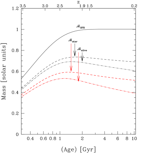
Figure 1: The mass content of a simulated galaxy is plotted as function of its age (bottom axis) and $z$ (assuming $z_{f}=4$, top axis). The black continuum line stands for the mass obtained by integration over the age of the model of a declining SFR with $\tau=0.4$ Gyr, normalized to the final total mass (in BC03 models, in column 9 of files .4color). Short dashed lines stand for the stellar mass still kept into stars at any age (i.e. it takes into account the stellar mass loss of some evolutionary phases, in BC03 models, in column 7 of files .4color). Dotted - short dashed lines stand for mass still kept into surviving stars alone (mass of dead remnants -e.g. in column 12 of files .3color in BC03 models - is subtracted). Black lines refer to models built with the Salpeter IMF, while red (grey) lines represent models obtained with Chabrier IMF (both assuming solar metallicity).

While $\mathcal{M}$_SFR is the same for different models since it depends only on the selected SF history, $\mathcal{M}$_star depends on the assumed IMF within the code, and on the stellar evolution picture on which the code itself is based. Figure 1 shows how different are the values corresponding to the three definitions of mass for the same model of galaxy and their dependence on the assumed IMF (Salpeter and Chabrier), in the case of a declining SFR with $\tau=0.4$ Gyr. For ages greater than few Gyr the mass still locked into stars is about 67% (50%) of the total mass involved in the past star formation activity, and only the 57% (35%) is that still locked into surviving stars for Salpeter (Chabrier) IMF. Smaller differences are produced by the assumption of different stellar tracks. Indeed, the same model reported above but built with the code Ma05 (replacing BC03 code) and Salpeter IMF has 72% of the total mass involved into past star formation activity locked into stars at ages of about 12-15 Gyr, and 61% locked into still alive stars, to be compared with 67% and 57% respectively as resulting from BC03 code.

In the following, we always refer to the total mass of the models expressed in equation (2), $\mathcal{M}$=$\mathcal{M}$_star, that is the most common definition adopted in recent works on stellar mass determinations (e.g., Fontana et al. 2006, van der Wel et al. 2006, Pozzetti et al. 2007). Since in the case of the SF histories which reasonably describe that of the early-type galaxies at ages greater than 1 Gyr $\mathcal{M}$_SFR is almost constant to its maximum value, we propose here some useful fits which allow to transform $\mathcal{M}$_star into $\mathcal{M}$_SFR for different IMFs and as a function of age (expressed in Gyr) and of z (assuming as formation redshift $z_{f}=4$) which are valid for exponentially declining SF histories with time scale $\tau\leq 0.8$ Gyr:

$$\mathcal{M}_{SFR}={\mathcal{M}_{star}\over[c_{0}^{age}-(0.01\times age)]}$$

$$\mathcal{M}_{SFR}={\mathcal{M}_{star}\over[c_{0}^{z}+(0.05\times z)]}$$

where $c_{0}^{age}$ is 0.75 assuming the Salpeter IMF and 0.65 for Kroupa and Chabrier IMFs, while $c_{0}^{z}$ is 0.62 for Salpeter IMF and 0.51 for Kroupa and Chabrier IMFs. The accuracy of the above equations is better than 10%, even if $z_{f}>4$.

3.2 Stellar mass: dependence on the model parameters

The conversion of a luminosity measure into a stellar mass estimate can be summarized by the following equation:

$$\mathcal{M}_{gal}[\mathcal{M}_{\odot}]=\mathcal{L}_{\lambda}^{gal}\ \mathcal{M/L}_{\lambda}$$ (4)

where $\mathcal{M}$_gal is the stellar mass of the galaxy expressed in solar masses, $\mathcal{L}_{\lambda}^{gal}$ is the luminosity of the galaxy at $\lambda$ in solar luminosities, and $\mathcal{M/L}_{\lambda}$ is the mass to light ratio at $\lambda$ in solar units. The luminosity of the galaxy $\mathcal{L}_{\lambda}^{gal}$ can be calculated from:

$$\mathcal{L}_{\lambda}^{gal}[\mathcal{L}_{\odot}]=10^{[-0.4(M_{\lambda}^{gal}-\ M_{\lambda}^{sun})]}$$ (5)

where $M_{\lambda}$ stands for the absolute magnitude at $\lambda$. If we merge the equations (4) and (5), and we consider that $M_{\lambda}^{gal}$ is derived from the apparent magnitude $m_{\lambda^{\prime}}^{gal}$, we obtain:

$$\log(\mathcal{M}_{gal})=\log(\mathcal{M/L}_{\lambda})+0.4kcor_{\lambda}+2\log(d_{pc})+\ \ \ \ \ \ \ \ \ \ \ \$$

$$\hfill-2.0+0.4M_{\lambda}^{sun}-0.4m_{\lambda^{\prime}}\ \ \$$ (6)

where $d_{pc}$ is the distance expressed in $pc$ that depends from the assumed cosmology and it is a function of $z$, $M_{\lambda}^{sun}$ is the absolute magnitude of the sun in the chosen filter centered at $\lambda$, while $m_{\lambda^{\prime}}$ is the apparent magnitude of the galaxy in the observed filter centered at $\lambda^{\prime}$. In Table 1 the most common values of $M_{\lambda}^{sun}$ for optical, near-UV and near-IR bands are given.

Table 1: Absolute magnitude of the Sun.

band $M_{\lambda}^{sun}$ Note U 5.61 a B 5.48 a V 4.83 a R 4.31 a I 4.02 a J 3.77 b H 3.45 b K 3.41 a

Note: (a) from the solar spectrum available at the CALSPEC database at STScI (Allen 1976); (b) values derived from $M_{K}^{sun}$ by means of colors calculated on the Kurucz synthetic spectrum G2 V.

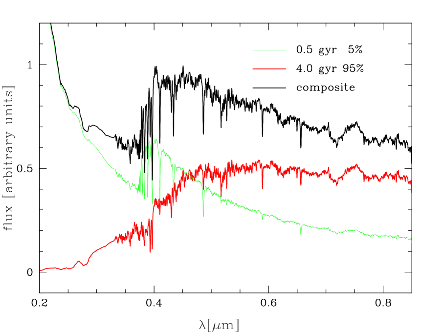
Figure 2: Thick black line: synthetic spectrum of a composite stellar population obtained by summing 95% of the mass of a 4 Gyr old population (thick grey/red line) and 5% of the mass of a 0.5 Gyr stellar component (thin grey/green line). Both the stellar populations correspond to solar metallicity and to the Salpeter IMF, and they have been derived from the exponentially declining star formation history with $\tau=0.4$ Gyr. The contribution to the total luminosity of the young SSP is more than 90% at $\lambda<0.3\mu m$, and similar to the contribution of the older much more massive component at $0.3\mu m<\lambda<0.5\mu m$. At $\lambda>0.5\mu m$ the contribution to the total luminosity of the young component is decreased down to less than 30%.

Spectrophotometric models are involved in the determination of two quantities of equation (6): i) the conversion factor $\mathcal{M/L}$ and ii) the k-correction needed to calculate the luminosity of the galaxy. In the following subsections, it will be demonstrated that the greatest accuracy in the determination of both the $\mathcal{M/L}$ ratio and the luminosity of galaxies is achieved in the near-IR bands. Indeed, optical blue and UV ranges (i.e. $\lambda<5000$ Å) are typically dominated by very luminous young stellar populations even when they represent few percentages of the total stellar content of the galaxies (see figure 2). In other words, the total stellar mass content is better traced by the near-IR luminosities because it does not depend on many details of the SF history followed by the galaxies. Moreover, the continuum shape of the near-IR spectral region is less dependent on the age of the stellar populations (see figure 2) with respect to the UV region, and this is why k-corrections (i.e. luminosities) can be determined with larger precision in the K band than in the V one.

3.2.1 Mass to light ratio: useful relations

The conversion factor between luminosities and stellar masses provided by the models ($\mathcal{M/L}$) depends first of all on the chosen wavelength band. Figures 3 and 4 show the value of $\mathcal{M/L}$ as a function of age and for different spectrophotometric codes, metallicities and SF histories, in the V and K band, respectively.

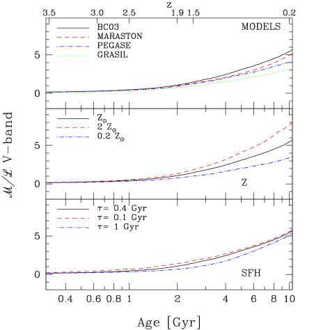
Figure 3: $\mathcal{M/L}$ ratio in the V band as a function of age (bottom axis) and $z$ (assuming $z_{f}=4$, top axis). In the top panel, results obtained with different codes for the same model galaxy are presented. The model galaxy has been built following an exponentially declining star formation rate with time scale $\tau=0.4$ Gyr at solar metallicity (Salpeter IMF), with the exception of the GRASIL code for which the Silva et al. (1998) reference model for elliptical galaxies has been considered (see details in §2.2). In the middle panel, the results obtained at three different values of metallicity are displayed. Models have been built adopting the BC03 code and the exponentially declining star formation rate ($\tau=0.4$ and Salpeter IMF). The bottom panel presents the results obtained assuming three different time scales of the declining star formation rate, for models built adopting the BC03 code at solar metallicity (Salpeter IMF).

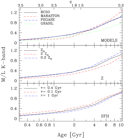
Figure 4: $\mathcal{M/L}$ ratio in the K band as a function of age (bottom axis) and $z$ (assuming $z_{f}=4$, top axis). The three panels show the effect of varying the code used to model the galaxies, the metallicity and the star formation history as in figure 3.

In both the two bands the largest variability of $\mathcal{M/L}$ is given by age variations, but what it should be noticed from the comparison of the two figures is the different y-axis scale that reveals a variation of $\mathcal{M/L}$ in the V-band of an order of magnitude against 50% of variation as a maximum of $\mathcal{M/L}$ in the K-band. In other words, small errors in the age assumed to reproduce the galaxies produce large errors in the resulting $\mathcal{M/L}$ in the optical bands, while have almost negligible effects in the determination of the $\mathcal{M/L}$ in the near-IR bands. For example, at solar metallicity, a standard early-type galaxy is characterized by $\Delta(\mathcal{M/L}_{V})/\Delta(age)=1.3$ and $\Delta$($\mathcal{M/L}$_K)/$\Delta(age)=0.2$ if age is expressed in Gyr. This means that an uncertainty of 1 Gyr in the age determination of a 4 Gyr old galaxy leads to an uncertainty in the $\mathcal{M/L}$ value of 0.2 in the K-band and of 1.3 in the V-band. For the above reason, it is strongly suggested to use near-IR bands luminosities when reliable mass estimates have to be derived.

Figures 4 and 5 contain all the dependencies of K-band $\mathcal{M/L}$ ratio on models and on their parameters. In particular, from the upper panel of figure 4 we can appreciate the small dependence of $\mathcal{M/L}$ on the spectrophotometric code (and implicitly on the possible different assumptions of the stellar tracks). Largest discrepancies are found between values obtained from Ma05 models with respect to BC03 ones. Indeed, K band $\mathcal{M/L}$ ratios from Ma05 models at ages lower than 2 Gyr reach values which are only 60% of those obtained with the BC03 code. This was expected since Ma05 models are brighter than the other models at ages between $\sim 0.2$ and $\sim 2$ Gyr, due to their different prescriptions of the TP-AGB phase and different isochrones adopted in the code (see §2.2). At the same time at old ages the values of $\mathcal{M/L}$ found by means of the Ma05 code are higher of a factor 1.2 than those found with the BC03 code. At old ages, large discrepancies are found also between the values of the K-band $\mathcal{M/L}$  ratios obtained with the GRASIL code with respect to the BC03 one. Indeed, the GRASIL values differ from the BC03 ones of a factor 0.8 at ages older than 7 Gyr, i.e. $z<0.5$. On the contrary, a better agreement is found between the PEGASE values and the BC03 ones over the whole range of ages/redshift.

The middle panel of figure 4 shows the dependence of $\mathcal{M/L}$_K on the stellar metallicity. The maximum difference between the values obtained at different metallicities is encountered at ages larger than 2 Gyr, when $\mathcal{M/L}$${}_{K}^{Z_{\odot}}$ is about 90% of $\mathcal{M/L}$${}_{K}^{0.2Z_{\odot}}$, and 1.2 times $\mathcal{M/L}$${}_{K}^{2Z_{\odot}}$. As an example, between $z=1$ and $z=2$, assuming $z_{f}=4$, $\mathcal{M/L}$_K varies from 0.6 to 0.3 for the effect of age variations while it varies from 0.5 to 0.7 (0.2 to 0.3) for metallicity variations at $z=1$ ($z=2$). Thus, at least in the ages/redshift range on which this work is focused, metallicity effects are of a second order with respect to the age effects.

The bottom panel of figure 4 confirms also a small dependence of $\mathcal{M/L}$ on the SF history selected to model the galaxy, at least for SF time scales smaller than 1 Gyr for which the variation of $\mathcal{M/L}$ is about 30% as a maximum. Figure 5 explores the dependence of $\mathcal{M/L}$  on the IMF for three different SF histories. It clearly appears that this parameter of the models is the main variable that produces uncertainty in the resulting value of $\mathcal{M/L}$. At the same time, the $\mathcal{M/L}$  values obtained within different IMFs have almost fixed ratios, so that we can consider different IMFs as different scaling factors for stellar mass calculations. In figure 5 we also report values obtained with the CB08 code and Chabrier IMF, which are systematically lower than those obtained with the same IMF but with the BC03 code. Indeed, this was expected, at least at young ages (i.e. $\sim 1-2$ Gyr) where the different treatment of the TP-AGB phase produces an increase of the luminosity with respect to the one derived with the BC03 code. Anyhow, we remember that the CB08 code is diffused in a preliminary version, and we wait for the authors publication on the details of the new code to more precisely understand this difference.

A complete summary of the results obtained with various models in the calculation of $\mathcal{M/L}$_K as a function of age and $z$ can be found at http://www.brera.inaf.it/utenti/marcella/. In particular, since $\mathcal{M/L}$ ratios in the near-IR bands are quite homogeneous and only slightly dependent on codes and details of the models used to calculate them, at the above address we suggest a set of reference values of $\mathcal{M/L}$_K as a function of $z$ and of the age of the galaxy, besides the parameters needed to transform $\mathcal{M}_{star}/\mathcal{L}$ into $\mathcal{M}_{SFR}/\mathcal{L}$ in case of exponentially declining SF history with time scale $\tau=0.4$ Gyr. In §3.3 we supply with an easy use of all those numbers, proposing the fit of $\mathcal{M/L}$_K as a function of age and of $z$ (assuming $z_{f}=4$).

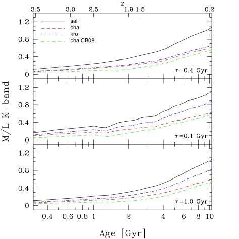
Figure 5: $\mathcal{M/L}$  ratio in the K band as a function of age (bottom axis) and $z$ (assuming $z_{f}=4$, top axis). The values obtained assuming different IMFs in the BC03 models (solar metallicity) are shown for exponentially declining models with $\tau=0.4$ Gyr (top panel), $\tau=0.1$ Gyr (middle panel) and $\tau=1.0$ Gyr (bottom panel). For comparison, results obtained assuming the Chabrier IMF but with the new version of the BC03 code (i.e. CB08) are displayed in all the three panels.

3.2.2 k-corrections: useful relations

k-corrections are needed to transform apparent magnitudes in the observed filter at $\lambda^{\prime}$ into absolute magnitudes in the same or another filter at $\lambda$:

$$kcor=-2.5\log{{\int{F_{z}(\lambda)S_{1}(\lambda)d\lambda}\over\int{F_{0}(\lambda)S_{2}(\lambda)d\lambda}}{\int{S_{2}(\lambda)d\lambda}\over\int{S_{1}(\lambda)d\lambda}}}\ \ \ \ \ \ \ \ \ \ \ \ \ \ \ \ \ \ \$$

$$\ \ \ \ \ \ \ \ \ \ \ \ \ \ \ \ \ \ \ \ \ \ +2.5\log(1+z)+(ZP_{S_{1}}-ZP_{S_{2}})$$ (7)

where $F_{z}(\lambda)=F_{0}(\lambda{1\over 1+z})$, S1 and S2 represent the observed and reference filters respectively, and ZP_i is the zero point for the filter ${i}$. In the definition of the classic k-correction S1 and S2 are coincident, and the definition can be simplified as:

$$kcor=-2.5\log{{\int{F_{z}(\lambda)S(\lambda)d\lambda}\over\int{F_{0}(\lambda)S(\lambda)d\lambda}}}+2.5\log(1+z)$$ (8)

while that defined in equation (7) is sometimes called colour k-correction.

Figures 6 and 7 show the classic k-corrections in the K and V bands respectively, as a function of age and for different models and models assumptions. The two figures do not display the effect obtained by varying the IMFs within the codes, because it has been found to be completely negligible. Figures 6 shows the high dependence of the near-IR k-corrections on stellar metallicity that is comparable to its dependence on age, while different SF histories display similar values. On the other hand, figure 7 makes evident that in the optical bands age remains the main variable driving the determination of the k-corrections (see the y-axis scale), while metallicity effects can be neglected. Moreover, there appears to be a large influence of even small variations in the stellar compositions of model galaxies, that we have displayed as dependence on the SF history. The absence of young components at age $<4$ Gyr for short SF time scale (e.g., $\tau=0.1$ Gyr) produces values which largely differ with the V band k-corrections calculated with models based on longer SF time scales.

As far as the different codes are concerned, we find again a different behavior of the k-corrections in the K band with respect to the V band. Indeed, the near-IR k-corrections values agree quite well among the different codes here analyzed, with the only exception of the Ma05 and CB08 models. In particular, PEGASE models return on average the same value of BC03 models within 0.96-1.17. On the other hand, the GRASIL models give K band k-corrections systematically smaller than the BC03 ones, but still within less than 20% (i.e., between 0.85 and 0.93). The Ma05 models on the contrary supply K band k-corrections values which, while at ages older than 3 Gyr (i.e. $z<1.5$) are larger than BC03 ones (within a factor 1.17), at young ages they become much smaller down to 50%. Even larger discrepancies are found between BC03 models and CB08 ones, giving the latter systematically smaller K band k-corrections down to 30% of the former. The latter two models are those which include more refined prescriptions for the TP-AGB phase which influence the continuum shape at young ages.

In the V band, the models which produce much different k-corrections values with respect to the others (up to 4 times the values of the other models) are those built with the GRASIL code. In fact, this reflects the different SF history that the GRASIL models assume with respect to the exponentially declining star formation rates with $\tau=$0.4 Gyr common to all the other models. Indeed, we have already noticed the large dependence of optical k-corrections on the SF history of the models. As far as the other models are concerned, they generally agree quite well with each other, with larger discrepancies found at intermediate ages (i.e. 2-5 Gyr, within a factor 1.3).

Summarizing, it can be said that the determination of the classic k-corrections in the optical bands present larger uncertainties because of their large variability ($\sim 5$ magnitudes) as a function of age, and of their large dependence on the assumed SF history. On the other hand, the near-IR bands k-corrections can be determined with larger accuracy because their variability is kept below 1.5 magnitudes for whatever parameter or model is varied. Their largest uncertainty is due to metallicity variations and to the choice of the code adopted to model galaxies between BC03, PEGASE and GRASIl codes on one hand and Ma05 and CB08 codes on the other one.

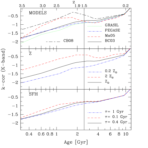
Figure 6: k-correction in the K-band as a function of age (bottom axis) and $z$ (assuming $z_{f}=4$, top axis). Panels display the effects of varying models, metallicity and star formation history as in figure 3.

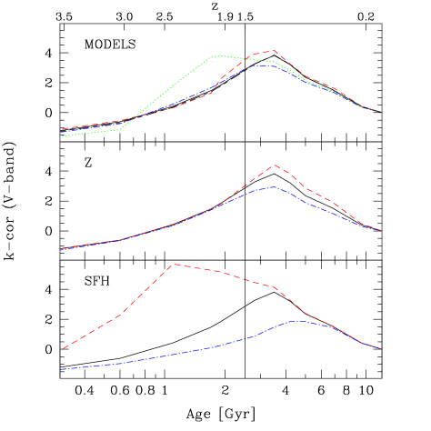
Figure 7: k-correction in the V-band as a function of age (bottom axis) and $z$ (assuming $z_{f}=4$, top axis). Panels display the effects of varying models, metallicity and star formation history as in figure 3

Figures 8 and 9 present the colour k-corrections in the K and V band, respectively. Colour k-corrections, defined as in equation (7), minimize the dependence on models and model parameters assuming a starting observed band as clos as possible to the rest frame band in which the absolute magnitude has to be calculated. In particular, the K band k-corrections have been derived from the observed bands from K to Spitzer 8$\mu$m, while the V band ones from V to K observed bands.

A complete summary of the results obtained with the different models in the calculation of the k-corrections in the V and K-band as a function of age and $z$ for different values of $z_{f}$ in the range between 4 and 10 can be found at http://www.brera.inaf.it/utenti/marcella/. As in the case of the $\mathcal{M/L}$ ratios, at the above address we also propose a set of reference values of both the classic and the colour k-corrections as a function of age [Gyr] and $z$. In §3.3 we supply with an easy use of all those numbers, proposing the fit of $k-$corrections in the K band as a function of age and of $z$ (assuming$z_{f}=4$).

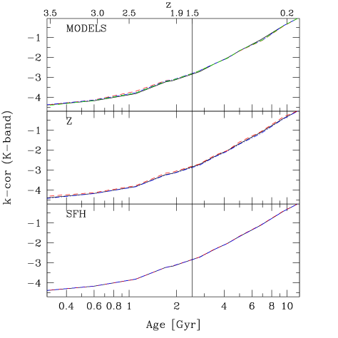
Figure 8: Colour k-correction in the K-band, obtained from the observed nearest band, from K to Spitzer 8.0$\mu$m filters.

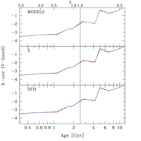
Figure 9: Colour k-correction in the V-band, obtained from the observed nearest band, from V to K filters.

3.2.3 Masses from apparent magnitudes: useful relations

In the previous two subsections, we have analyzed the behavior of the parameters $\mathcal{M/L}$ and k-corrections as a function of models and model parameters, suggesting the use of near-IR bands. We have also seen that IMFs, metallicities and codes at a fixed age can produce values of one or both of the two quantities which differ by a large amount with respect to the reference values. In this section, we want to check the behavior of the combination of the two quantities included in the formula that transforms apparent magnitudes into stellar masses (see equation 6):

$$\log(\mathcal{M/L})+0.4kcor$$

Figure 10 shows the behavior of such quantity as a function of age [Gyr] and $z$ (assuming $z_{f}=4$), for different combinations of models and IMFs. In particular, it is remarkable that the values of this quantity calculated with Ma05 code and Salpeter IMF well agree with the values which can be calculated with BC03 models. Indeed, the difference between the two codes as far as the combination of k-corrections and $\mathcal{M/L}$ in the K band are concerned turns out to produce differences in the mass estimates at fixed apparent magnitude which are of less than 20% (between a factor 0.9-1.2) as a maximum and which are on average less than 5%. Something similar happens with the values calculated with CB08 code compared with the values calculated with BC03 code and Chabrier IMF (see top panel of figure 10). The differences between the two codes turn out to produce differences in the stellar masses which are within a factor 0.8-1.2. At the same time, from the middle panel it is evident that a larger discrepancy in the mass estimate can arise within models built with the same code but with different metallicities. Adopting models with $Z=0.2Z_{\odot}$ mass estimates (at fixed age) result on average less than 80% of the mass estimates derived assuming solar metallicity, while if $Z=2.5Z_{\odot}$ mass estimates result on average a factor 1.4 higher than the estimates at solar metallicity.

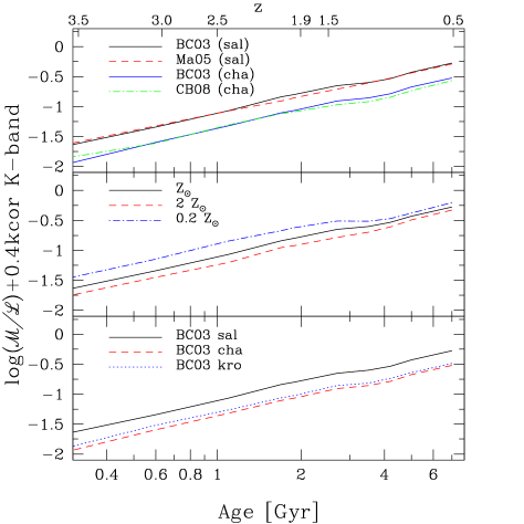
Figure 10: The quantity $\log(\mathcal{M/L})+0.4kcor$ is plotted as a function of age (bottom axis) and $z$ (assuming $z_{f}=4$, top axis). The upper panel compares values calculated with different models at solar metallicity, the middle panel compares values obtained with BC03 models at different metallicities, and the lower panel compares values obtained with BC03 model at solar metallicity but with different IMFs.

3.3 Stellar mass from different codes and parameters

Details of the dependence of $\mathcal{M/L}$ rations and k-corrections on models and model parameters have been described in the previous subsections, and many tables which summarize the corresponding values as a function of age and $z$ for different values of $z_{f}$ in the range between 4 and 10 can be found at http://www.brera.inaf.it/utenti/marcella/. Here we supply with an easy use of all those numbers, proposing the fits of some quantities as a function of age and of $z$ for $z_{f}=4$. In particular, Table 2 reports the values of the coefficients $a_{i}$ of the following expressions:

$$[\mathcal{M/L}_{K}]_{Y}=a_{0}+a_{1}\times age+a_{2}\times age^{2}+a_{3}\times age^{3}$$ (9)

$[\mathcal{M/L}_{K}]_{Y}=a_{0}+a_{1}\times z+a_{2}\times z^{2}+a_{3}\times z^{3}\hfill(9b)$

where Y stands for the following combinations of models and IMFs: i) Salpeter IMF and all the models excluded the CB08 and Ma05 ones, ii) Salpeter IMF and Ma05 model, iii) Chabrier IMF and BC03 model, iv) Chabrier IMF and CB08 model, v) Kroupa IMF and BC03 model. Note that the combination Salpeter IMF and Ma05 model, and Chabrier IMF and CB08 model have been proposed separated from the other fits for the same IMF because they supply quite different values of the $\mathcal{M/L}$ ratio contrary to the homogeneity (within 20%) of the results achieved with the other models. The fits minimize the percentage difference between the polynomial expressions of equations 9 and 9b and the exact values, and they are all stopped to the minimum order that returns on average the exact values within 5%. As an example aimed at showing the accuracy of the fits mentioned above, one can consider that a galaxy at $z=1.0$ with age=4.2 Gyr would result having $[\mathcal{M/L}_{K}]^{Sal}=$ 0.57, as average from BC03, PEGASE and GRASIL models. The values resulting from the fits are 0.57 and 0.58 as a function of age and of $z$, respectively. The same galaxy would have $[\mathcal{M/L}_{K}]^{Cha}=$ 0.35 and 0.36 and $[\mathcal{M/L}_{K}]^{Kro}=$ 0.37 and 0.39 (as a function of age and $z$, respectively) to be compared with the values derived from BC03 models equal to 0.32 and 0.36. The accuracy of the fit with respect of the $\mathcal{M/L}$_K derived by the single models can be seen in Figure 11 (top panel) for the case i) as a function of $z$. Values derived with the Ma05 code are also reported for comparison, and it can be noticed that they are higher at low redshift and lower at high redshift.

Table 3 reports the values of the coefficients $a_{i}$ of the following expressions:

$$kcor_{Y}=a_{0}+a_{1}\times age+a_{2}\times age^{2}+a_{3}\times age^{3}+a_{4}\times age^{4}$$ (10)

$kcor_{Y}=a_{0}+a_{1}\times z+a_{2}\times z^{2}+a_{3}\times z^{3}+a_{4}\times z^{4}\hfill(10b)$

where Y stands for the following combinations of models and $Z$ values: i) all the models excluded CB08 and Ma05 at solar metallicity, which result homogeneous within less than 10%, ii) all the models excluded CB08 and Ma05 at $z=0.2Z_{\odot}$, iii) all the models excluded CB08 and Ma05 at $z=2.5Z_{\odot}$, iv) Ma05 model at solar metallicity and v) CB08 model at solar metallicity. Note that k-corrections depend on the metallicity of the stellar populations but not on the IMF used to model them. Furthermore, Ma05 and CB08 models supply quite different values of k-corrections in the K band, and thus separated fits have been proposed for these models.

Table 2: Coefficients of the fits of $\mathcal{M/L}$_K as a function of age [Gyr] and $z$ ($z_{f}=4.0$): $[\mathcal{M/L}_{K}]_{Y}=a_{0}+a_{1}\times$ age $+a_{2}\times$age${}^{2}+a_{3}\times$age³ and $[\mathcal{M/L}_{K}]_{Y}=a_{0}+a_{1}\times z+a_{2}\times z^{2}+a_{3}\times z^{3}$ where Y stands for the following combinations: i) Salpeter IMF and all the models excluded CB08 and Ma05, ii) Salpeter IMF and Ma05 models, iii) Chabrier IMF and BC03 models, iv) Chabrier IMF and CB08 models, v) Kroupa IMF and BC03 models. Note that the combinations of Salpeter IMF with the Ma05 model, and Chabrier IMF with CB08 model have been proposed separated from the other fits for the same IMFs because they supply quite different values of the $\mathcal{M/L}$ ratio contrary to the homogeneity of the results achieved with the other models.

$a_{0}$ $a_{1}$ $a_{2}$ $a_{3}$ $\chi^{2}$ $a_{0}$ $a_{1}$ $a_{2}$ $a_{3}$ $\chi^{2}$ $[\mathcal{M/L}_{K}]_{Y}=a_{0}+a_{1}\times$ age $+a_{2}\times$ age${}^{2}+a_{3}\times$ age³ $[\mathcal{M/L}_{K}]_{Y}=a_{0}+a_{1}\times z+a_{2}\times z^{2}+a_{3}\times z^{3}$ i) Salpeter IMF 0.07 0.14 -0.005 0.0000 0.01 0.96 -0.43 0.054 0.0000 0.03 ii) Salpeter IMF - Ma05 0.12 0.00 0.041 -0.0032 0.07 1.42 -1.04 0.266 -0.0211 0.02 iii) Chabrier IMF - BC03 0.03 0.10 -0.008 0.0004 0.03 0.67 -0.47 0.146 -0.0178 0.05 iv) Chabrier IMF - CB08 0.04 0.02 -0.0104 0.00078 0.04 0.64 -0.522 0.1647 -0.01814 0.04 v) Kroupa IMF - BC03 0.04 0.11 -0.010 0.0005 0.04 0.61 -0.26 0.031 0.0000 0.07

Table 3 proposes also the fit of the colour k-corrections between observed 4.5$\mu$m Spitzer band and rest frame K-band that stands for ages younger than 7 Gyr and/or $z>0.2$ (see details and definitions in §3.2.2) which almost do not depend on the choice of the models and on the metallicity of the stellar populations. Following the same example as before, a galaxy at $z=1.0$ with age=4.2 Gyr, at solar metallicity would result having $kcor$= -0.77 as average value of those derived from the BC03, PEGASE and GRASIL models. The values resulting from the fits are -0.75 and -0.73 as a function of age and of $z$, respectively. The same galaxy at $Z=0.2Z_{\odot}$ would have $kcor$= -0.93 in the BC03 models to be compared with the values of -0.95 and -0.90 resulting from the fits as function of age and $z$, respectively. As in the case of $\mathcal{M/L}$_K, we report an example of comparison between data and fit of eq (10b) in the middle panel of figure 11. Points derived from the Ma05 code are also reported and it can be noticed that at low ages (e.g. high redshift) they are much higher than the average of the values obtained with the other models.

Table 3: Coefficients of the fits of K-band k-corrections as a function of age [Gyr] and $z$ ($z_{f}=4.0$): $kcor_{Y}=a_{0}+a_{1}\times$ age $+a_{2}\times$age${}^{2}+a_{3}\times$ age${}^{3}+a_{4}\times$ age⁴ and $kcor_{Y}=a_{0}+a_{1}\times z+a_{2}\times z^{2}+a_{3}\times z^{3}+a_{4}\times z^{4}$ where Y stands for the following combinations: i) all the models excluded CB08 and Ma05 at solar metallicity, ii) all the models excluded CB08 and Ma05 at $z=0.2Z_{\odot}$, iii) all the models excluded CB08 and Ma05 at $z=2.5Z_{\odot}$, iv) Ma05 model at solar metallicity and v) CB08 model at solar metallicity. Note that Ma05 and CB08 models supply quite different values of k-corrections in the K band, and thus separated fits have been proposed. The last two lines list the coefficients of the same fits above but for the colour k-corrections between observed 4.5$\mu$m Spitzer band and rest frame K-band that stand for ages younger than 7 Gyr and/or $z>0.2$ which almost do not depend on the choice of the models and on the metallicity of the stellar populations.

$a_{0}$ $a_{1}$ $a_{2}$ $a_{3}$ $a_{4}$ $\chi^{2}$ $a_{0}$ $a_{1}$ $a_{2}$ $a_{3}$ $a_{4}$ $\chi^{2}$ $kcor_{Y}=a_{0}+a_{1}\times$ age $+a_{2}\times$age${}^{2}+a_{3}\times$ age${}^{3}+a_{4}\times$ age⁴ $kcor_{Y}=a_{0}+a_{1}\times z+a_{2}\times z^{2}+a_{3}\times z^{3}+a_{4}\times z^{4}$ i) $Z=Z_{\odot}$ -1.95 0.84 -0.192 0.0143 0.0000 0.03 -0.32 -0.65 0.314 -0.0735 0.0000 0.01 ii) $Z=0.2Z_{\odot}$ -2.17 0.77 -0.159 0.0115 0.0000 0.02 -0.35 -0.81 0.309 -0.0636 0.0000 0.01 iii) $Z=2.5Z_{\odot}$ -1.76 1.67 -0.703 0.1162 -0.00655 0.01 0.66 -3.39 3.200 -1.1595 0.13606 0.03 iv) Ma05 $Z=Z_{\odot}$ -2.18 2.45 -1.258 0.2429 -0.01554 0.07 0.20 -2.46 1.828 -0.4484 0.02245 0.01 v) CB08 $Z=Z_{\odot}$ -2.10 2.50 -1.1782 0.2124 -0.01291 0.07 0.98 -4.90 4.805 -1.7598 0.20933 0.07 $m(4.5\mu)_{z}-m(K)_{z=0}=kcor$ $kcor_{Y}=a_{0}+a_{1}\times$ age $+a_{2}\times$age${}^{2}+a_{3}\times$ age${}^{3}+a_{4}\times$ age⁴ $kcor_{Y}=a_{0}+a_{1}\times z+a_{2}\times z^{2}+a_{3}\times z^{3}+a_{4}\times z^{4}$ -3.32 0.33 -0.004 0.0000 0.00000 0.01 -0.43 -1.81 0.300 0.0000 0.00000 0.02

Finally, before concluding this section, we want to propose a very simple way to obtain stellar mass estimates of early-type galaxies that combines the results retrieved above on the $\mathcal{M/L}$ ratio and k-corrections in the K band. Indeed, we have seen that for fixed IMF $\mathcal{M/L}$_K and luminosities (by means of k-corrections) only slightly depend on the specific code used to derived them, and their largest dependence is on age and $z$ of the stellar populations. This means that for a given apparent luminosity, stellar mass can be derived just as function of $z$ if we assume that age itself is a function of $z$ (e.g. $z_{f}=4$). Thus, we propose the following equations:

—————————————————————————

$$log[\mathcal{M}^{Sal}(z)]=[-0.4\times m_{K}]+[17.45+1.22z-0.25z^{2}]$$ (11)

$log[\mathcal{M}^{Sal}(z)]=[-0.4\times m_{4.5}]+[17.52+0.49z-0.10z^{2}]\hfill(11b)$

—————————————————————————

to derive $\mathcal{M}$ from the apparent K band magnitude $m_{K}$ (eq. 11) or 4.5$\mu$m band magnitude (eq. 11b), and from the redshift $z$, assuming Salpeter IMF. Equations (11) and (11b) return a mass estimate that results within 0.15 dex of the value that could be obtained adopting all the models and the metallicities discussed in the previous section (i.e. within a factor between 0.7-1.4), including the Ma05 and CB08 models (see the discussion in §3.2.3). Indeed, Figure 11 (bottom panel) displays for all the models listed above (Salpeter IMF) the values of $\log(\mathcal{M/L}_{\lambda})+0.4kcor_{\lambda}+2\log(d_{pc})+-2.0+0.4M_{\lambda}^{sun}$ as a function of the redshift $z$, which show a large homogeneity contrary to the larger discrepancies found in the values of $kcor$ and of $\mathcal{M/L}$.

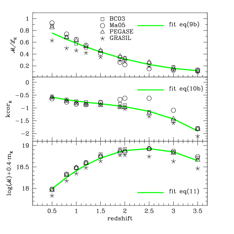
Figure 11: Top panel: $\mathcal{M/L}$ ratio in the K band for different models (Salpeter IMF) as a function of $z$. The thick grey (green) line shows the fit of the data as in eq. (9b), where the coefficients have been taken from Table 2 case i). Middle panel: k-correction in the K band for different models (solar metallicity) as a function of $z$. The thick grey (green) line shows the fit of the data as in eq. (10b), where the coefficients have been taken from Table 3 case i). Bottom panel: the $z$-dependent part of the formula used to calculate stellar masses (see eq. 6) from apparent K band magnitude $\log(\mathcal{M/L}_{\lambda})+0.4kcor_{\lambda}+2\log(d_{pc})+-2.0+0.4M_{\lambda}^{sun}$ is shown as a function of $z$, for different models (Salpeter IMF and solar metallicity). The thick grey (green) line shows the fit of the data as in eq. (11).

Figure 12: The stellar mass M_others for a sample of 69 ETGs derived from the best fitting to their SEDs is compared with the mass $\mathcal{M}^{(eq.11)}$ derived by eq. (11). The 69 ETGs come from the samples of Rettura et al. (2006, 40 ETGs) and of Saracco et al. (2008, 29 ETGs). The mass $\mathcal{M}^{(eq.11)}$ has been scaled to the same IMF used by the authors using eqs. (12) and (13). The solid lines represent the relation M${}_{others}=\mathcal{M}^{(eq.11)}$. For 55 out of the 69 ETGs the two estimates of the mass agree within a factor 2 (dotted lines, lower panel).

For instance, a galaxy at $z=1$ and age=4.2 Gyr with $m_{K}$=18.5 would result having $1.0\cdot 10^{11}\mathcal{M}_{\odot}$, to be compared with $1.2\cdot 10^{11}\mathcal{M}_{\odot}$ for BC03 models, $1.2\cdot 10^{11}\mathcal{M}_{\odot}$ for Ma05 models, $1.2\cdot 10^{11}\mathcal{M}_{\odot}$ for PEGASE models and $0.9\cdot 10^{11}\mathcal{M}_{\odot}$ for GRASIL models. At higher redshift, a galaxy at $z=2$ and age=1.2 Gyr with $m_{K}$=19.0 would result having $1.9\cdot 10^{11}\mathcal{M}_{\odot}$, to be compared with $2.1\cdot 10^{11}\mathcal{M}_{\odot}$ for BC03 models, $1.8\cdot 10^{11}\mathcal{M}_{\odot}$ for Ma05 models, $1.9\cdot 10^{11}\mathcal{M}_{\odot}$ for PEGASE models and $1.5\cdot 10^{11}\mathcal{M}_{\odot}$ for GRASIL models.

It is worth noting that the above equations are based on the assumption of $z_{f}=4$. On the other hand, results would continue to be in good agreement with those of equations 11 and 11b in case, for instance, of the assumption $z_{f}=6$. Indeed, the higher formation redshift means that galaxies at the same $z$ are about 0.5 Gyr older, and the corresponding k-corrections are less than 0.1 magnitudes higher. This difference in the value of the k-corrections leads to a mass estimate that is 90% of the value obtained with $z_{f}=4$ as a maximum, that is well within the range 0.7-1.4 that is the uncertainty of equations 11 and 11b.

Masses obtained assuming Salpeter IMF can be simply converted into those with Chabrier and Kroupa IMF adopting the following expressions:

$$[\mathcal{M}^{Cha}(z)]=0.55\times[\mathcal{M}^{Sal}(z)]$$ (12)

$$[\mathcal{M}^{Kro}(z)]=0.62\times[\mathcal{M}^{Sal}(z)]$$ (13)

The conversion of $\mathcal{M}^{Sal}$ into $\mathcal{M}^{Cha}$ proposed above by means of a constant independent of $z$ gives results which are within 10% in agreement with those obtained from BC03 models. $\mathcal{M}^{Cha}$ obtained by means of the new CB08 models are lower than those obtained by means of BC03 models (between 70% and 80%) and thus lower than the values resulting from equations (11) and (12) but still within 20%. Finally, $\mathcal{M}^{Kro}$ resulting from equations (11) and (13) agrees within 10% with the values obtained by means of BC03 models with Kroupa IMF.

As a simple exercise, we compared the stellar mass derived from eq. (11) based on the apparent K-band magnitude with the mass estimated from the SED fitting for a sample of 69 ETGs at $0.5<z<2$ with spectroscopic confirmation of their redshift and spectral type. This sample includes 29 out of the 32 ETGs studied by Saracco et al. (2008) and 40 ETGs taken from the compilation of Rettura et al. (2006) including some ETGs of the sample of van der Wel et al. (2005) and of di Serego Alighieri et al. (2005). The 29 ETGs taken from Saracco et al. (2008) have stellar masses obtained with Chabrier IMF while those from Rettura et al. (2006) are based on Kroupa IMF. To compare these masses with those derived from eq. (11) tuned on Salpeter IMF we used eqs. (12) and (13) to scale them to the same IMF. The comparison is shown in Fig. 12 where the original mass M_others provided by the other authors is plotted versus the mass $\mathcal{M}^{(eq.11)}$ (upper panel). In the lower panel the ratio between the two masses is shown. The agreement between them is remarkable: for 55 out of the 69 ETGs (80% of the sample) the two masses agree within a factor 2 while they agree within a factor 3 for 66 ETGs (96% of the sample).

4 The best fitting technique applied to early-type galaxies at $1<z<2$

The previous section has described the differences of the mass estimates obtained with different codes or different parameters within the same code at fixed age and redshift. But when multi-wavelength photometric data are available, age is not associated a priori to the galaxies. On the contrary, models are used to build libraries of spectral templates which are adopted to find the one best fitting the whole SED of the galaxies. In the best fitting technique, age is the fundamental parameter that is determined and that fixes the model reproducing the observed SED of the galaxy. With the aim to assess the reliability of the estimates of the main physical properties of early-type galaxies at $1<z<2$ derived by the technique of best fitting a wide set of photometric data, we apply it to a set of simulated galaxies for which the input properties are known. We then compare the obtained results with the known true values, focusing our attention on the stellar mass estimate and its dependence on the different mass estimators used to derive it. We want to emphasize here that the following analysis considers results obtained by means of photometric data only, while possible spectroscopic information could in principle allow to obtain better results.

Table 4: Model parameters for the mock catalogs. The symbol X marks the combinations among ages, redshift and times of the secondary burst which have been considered.

ages [Gyr] $z=1.0$ 4.2 3.0 2.7 2.0 1.7 no burst X X X X X at $t=0.6$ Gyr X X X X X at $t=1.7$ Gyr X X X X at $t=2.7$ Gyr X X at $t=3.5$ Gyr X $z=1.5$ 4.2 3.0 2.7 2.0 1.7 no burst X X X X at $t=0.6$ Gyr X X X X at $t=1.7$ Gyr X X X at $t=2.7$ Gyr X at $t=3.5$ Gyr $z=2.0$ 4.2 3.0 2.7 2.0 1.7 no burst X X at $t=0.6$ Gyr X X at $t=1.7$ Gyr X at $t=2.7$ Gyr at $t=3.5$ Gyr

As a first step, we built three mock photometric catalogs of galaxies, whose properties in terms of wavelength coverage and photometric accuracy have been simulated according to those of two main current surveys, the VIMOS VLT Deep Survey (VVDS, Le Fevre et al. 2005) and the Great Observatories Origins Deep Survey (GOODS) for which we adopted the MUSIC sample (Grazian et al. 2006). It is worthy to note that our aim is just to use the properties of these two surveys to simulate the observations of a sample of early-type galaxies, and not to reproduce the observed surveys themselves. In particular, the wavelength coverage of two of our three mock catalogs corresponds to the photometric bands in common to the two original catalogs, that are U, B, V, I, J and K, even if filters slightly differ among the two surveys due to different instruments used for the observations (e.g. B, V and I band of the GOODS catalog are from HST-ACS F435W, F606W and F775W filters, while the same bands in the VVDS are derived from observations with the Canada-France Telescope and CFH12k mosaic camera). A third mock catalog adds to these six photometric bands the four Spitzer-IRAC IR bands (3.6$\mu$m, 4.5$\mu$m, 5.8$\mu$m and 8.0$\mu$m) which are included in the original MUSIC GOODS catalog. As far as the photometric accuracy is concerned, we reproduced that of the two surveys in each band and in bins of 1 magnitude, for selected objects in the original catalogs with redshift $z>1$. Figure 13 shows the errors associated to each bin of magnitude in each of the 6 bands. The errorbars display the dispersion found around the average values of the errors, and they depend on the number of objects populating each bin of magnitude in each of the two catalogs. Since the photometric accuracy only depends on the observed apparent magnitude and not on the spectral type of the observed galaxies, we adopted the full VVDS and GOODS original catalogs to calculate the expected errors.

The expected magnitudes in all the filters of the three mock catalogs are calculated on a set of model templates whose parameters reproduce the properties of early-type galaxies at $1<z<2$, assuming the BC03 code at solar metallicity and with Salpeter IMF. The assumed SF history is described by an exponentially declining SFR with time scale $\tau=0.6$ Gyr. The possibility of secondary star forming episodes is taken into account by the superimposition of $\tau=0.1$ Gyr models on the principal SF history at different times assuming their contribution to the final total stellar mass as equal to 5% and to 20%. The chosen combinations among ages, redshift and times of the secondary burst (which are summarized in Table 4) constitute 57 template spectra, among which 11 with no secondary star forming episodes and 16 with recent (i.e. $<1$ Gyr) starburst, half of which forms 5% of the total final mass while the contribution of the other half is 20%.

Finally, the stellar mass content of the simulated galaxies, needed to calculate their apparent magnitudes as a function of their redshift, has been fixed as $0.3,1.0,3.0\times 10^{11}$ M_⊙, and the possibility of dust obscuration has been taken into account assuming A${}_{V}=0.0,0.2,0.5$ and the reddening law of Calzetti et al. (2000). In the catalogs we did not include the exact values of the calculated apparent magnitudes, but values randomly generated following a gaussian distribution probability around the exact value and with $\sigma$ equal to the assumed photometric errors.

The photometric catalogs of the simulated galaxies have been compared with those of real samples of early-type galaxies, in order to test the reliability of the simulations. The comparison sample has been collected considering the early-type galaxies found in the GOODS catalog, following their spectral classification as reported by the last release of the spectroscopic catalog of GOODS (Vanzella et al. 2008) and/or by the K20 catalog (Mignoli et al. 2005). Since most of the GOODS galaxies spectrally classified as early-types are at $z<1.2$, we added some data of early-type galaxies at higher redshift selected from the compilation of Saracco et al. (2008; see http://www.brera.inaf.it/utenti/saracco/), for a total sample of 125 galaxies in the redshift range $0.6<z<2.2$. Figure 14 (upper panels) shows the comparison of some colours of the simulated galaxies (reported as filled symbols) with those observed (crosses and open circles). In particular, the left panel displays the (V-K) vs. (V-I) colors, while the right panel proposes the (V-K) vs. (J-K) colours. The arrows in the right-bottom portion of each panel displays the direction along which a galaxy move in these diagrams when the redshift, the age and the extinction are increased. As it can be seen, the simulated galaxies well covers the parameter space of the observed galaxies.

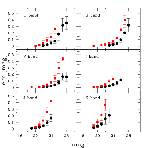
Figure 13: Observed photometric errors associated to the measured magnitudes in VVDS (grey/red filled squares) and GOODS (black filled circles) original catalogs. The errorbars represent the dispersion of the distribution of errors in each bin of magnitudes.

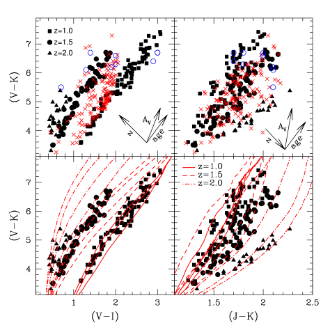
Figure 14: Colour-colour diagrams of the simulated galaxies compared with a sample of observed galaxies (top panels) and with models used to build the template spectral library adopted in the best fitting procedure with hyperz (see details in the text) (lower panels). Simulated galaxies are reported as filled symbols, which are squares for $z=1.0$, circles for $z=1.5$ and triangles for $z=2.0$. Observations coming from the GOODS sample are reported as crosses, while higher redshift data from Saracco et al. (2008) are reported as open circles. Models sequences are reported as continuum lines (models at $z=1$), dashed line (models at $z=1.5$), and dashed-dot lines (models at $z=2$). The arrows in the right-bottom portion of each panel display the direction along which a galaxy move in these diagrams when the redshift, the age and the extinction are increased.

As a second step, we applied the best fitting technique to our three mock catalogs by means of the photometric redshift code hyperz (Bolzonella et al. 2000). The code compares within a given range of redshift a set of spectral templates with the observed photometric magnitudes and their uncertainties, varying the free parameters: star formation time scale $\tau$, age, dust extinction. The spectral library adopted to find the best fitting template for each galaxy is composed by exponentially declining star formation models with time scales $\tau=0.1,0.3,0.6,1.0$ Gyr, at solar metallicity. They have been generated by means of the BC03 code, assuming Salpeter IMF. In the best fitting procedure the extinction has been allowed to vary between A${}_{V}=0.0$ and A${}_{V}=0.5$ and at each $z$ ages have been forced to be lower than the Hubble time at that $z$. Assuming that the redshift is known within 0.1, we run the code with $z$ varying between +/- 0.05 of its true value. The assumed set of parameters reproduces the choices generally made to study the photometric properties of real early-type galaxies with known spectroscopic redshift (e.g. Longhetti et al. 2005). It can be noted that the set of parameters chosen to find the best fit of our simulated galaxies in some cases exactly covers the range of parameters adopted to simulate the galaxies (e.g. A_V values, IMF, metallicity), in other cases it covers a smaller range (e.g. SF histories). Independently of the incompleteness of the parameters adopted to build it, the template library allows to well cover the colours of the simulated early-type galaxies. As an example, the lower panels of figure 14 show the comparison of two colours sequences of the models adopted as template library in hyperz with the colours of the simulated mock catalogs.

Finally, once a best fitting template has been associated to each simulated galaxy, we have estimated its luminosity, its $\mathcal{M/L}$ ratio and its stellar mass content as derived from the parameters of the best fitting template itself. The obtained values have been then compared with the true known input values of the same parameters defining the model used to simulate the galaxies of the mock catalogs. In the following, we analyze in details this comparison, for different bands and different estimators both of luminosity and of stellar mass, while in Appendix A the same comparison is analyzed for the $\mathcal{M/L}$ parameter.

4.1 Luminosity in the K and V bands

We derived $M_{K}$ and $M_{V}$ absolute magnitudes in the K and V bands respectively, from the apparent $m_{V}$ and $m_{K}$ magnitudes, applying the k-corrections calculated on the best fitting templates, and the dust corrections $dcor$ derived from the best fit values of A_V, besides the distance modulus:

$$M=m-d\_mod(z)-kcor(\lambda)-dcor(\lambda)$$

where $m$ is the apparent magnitude, $d\_mod$ is the distance modulus ($d\_mod=5\log(d_{Mpc})+25$) and $kcor(\lambda)$ and $dcor(\lambda)$ are the k-correction and the extinction correction depending on the wavelength of the photometric band. We also calculated $M_{K_{4.5}}$ and $M_{V_{J}}$ which are K and V band absolute magnitudes derived from the apparent 4.5$\mu$m and J band fluxes respectively, i.e. from the observed bands closer to their rest frame wavelengths. Finally, we define $M_{K_{raw}}$=$m-d\_mod(z)-kcor_{raw}$ where $kcor_{raw}$ is the value calculated by means of equation (10b) and assuming the coefficients from Table 3 relative to the case i) valid for $Z=Z_{\odot}$ and all the models except Ma05 and Cb08 ones (i.e. first line, right part of the table).

Figure 15 describes the uncertainties of the luminosity estimators introduced above. The average value of the difference between the absolute magnitudes as recovered by the estimators and their true values are reported as empty points, while the errorbars mark the maximum differences between the same quantities. Square points refer to luminosity estimators which use the template best fitting the available photometric data to derive the corresponding k-correction, while the circle refers to $M_{K_{raw}}$ that does not need any multi-wavelength data fitting. For comparison, we report also the range of uncertainties of the apparent magnitude used to derive the absolute one (shaded areas). As far as the K band is concerned, K band magnitudes are generally recovered within 0.2-0.3 magnitudes in the case of both the two GOODS mock catalogs ($\Delta$K$<0.1$), while due to larger errors in the apparent magnitudes ($\Delta$K=0.2-0.3) the uncertainty is around 0.5 magnitudes in the case of the VVDS mock catalog, and it can raise to more than 1.0 magnitude in the case of the fainter objects (i.e. with $\mathcal{M}$${}_{star}=0.3\times 10^{11}$M_⊙ at $z=2$). Spitzer IR data with small errors ($\Delta$(4.5$\mu$m)$<$0.1) allow to obtain estimates of the K band magnitudes even better than 0.2 magnitudes. It is particularly remarkable that the K_raw value of the K band magnitude is well determined within 0.3-0.4 magnitudes when the apparent K band magnitudes are affected by small errors ($\Delta$K$<0.1$) and within 1 magnitude for the larger errors of the fainter objects in the VVDS mock catalog. This demonstrates the easiness to derive a reliable estimate of the near-IR luminosities for early-type galaxies at known redshift. Moreover, all the estimators of the K band magnitudes produce results which are distributed around the true values and systematic offset larger than few hundredths are not apparent.

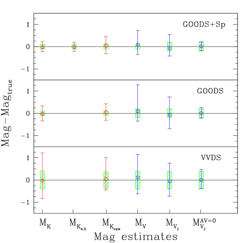
Figure 15: Uncertainties in the estimates of the absolute magnitudes in the K and V band. The reported errorbar represents the whole range of values spanned by the difference between the true and the recovered magnitudes. Dots are the average values of the same difference. Square dots refer to luminosity estimators which use the best fitting template of the available photometric data to derive the corresponding k-correction, while the circle refers to $M_{K_{raw}}$ that uses a value of $kcor$ derived by equation (10b) that does not need any multi-wavelength data fitting. The shaded areas highlight the range of uncertainties of the apparent magnitudes used as the starting point to derive the absolute ones.

This is not the case in the V band, for which the value of $M_{V}$ statistically underestimates the true luminosities of the simulated galaxies of more than 0.1 magnitudes. Furthermore, the recovered values of $M_{V}$ show large differences with the true V absolute magnitudes, i.e. larger than 1 magnitude. The reason of the underestimate of the V luminosities is in the general underestimate of the k-correction in this band (due to the trend of a slightly overestimate of the age parameter), and at the same time its large uncertainty is due to the large uncertainty in the k-correction and dust correction determination. When $V_{J}$ is used to estimate the V luminosity, the uncertainty due to the determination of the correct k-correction value disappears, and the uncertainty due to the bad dust correction determination leads to slightly overestimate on average the V band luminosity. The last bar closest to the right border of figure 15 represents results obtained assuming $A_{V}=0$ in hyperz for models which do not include dust. $V_{J}^{A_{V}=0}$ retrieves the V absolute magnitude within 0.3-0.4 magnitudes for the VVDS mock catalog, and 0.2 for the GOODS mock catalog, that is within the uncertainties affecting the measured J band apparent magnitudes. When real galaxies are observed, no information on the effective dust content is known a priori, and thus the last results obtained fixing A${}_{V}=0$ both in models and in the templates used to analyze them is a simple exercise to understand the behaviour of our optical magnitude estimates but it cannot be considered representative of any serious data analysis.

Summarizing, for the same goodness of the best fit selected to represent the observations, the uncertainties in the determination of the V absolute magnitude are much larger than in the K band. In other words, it is easier to obtain a good determination of near-IR absolute luminosities than optical ones.

4.2 Stellar masses from different estimators

Stellar mass content of the simulated galaxies has been recovered by means of several different mass estimators:

$\bullet$ $\mathcal{M}_{b}$ derives stellar masses from the scaling parameter $b$ of hyperz. The parameter $b$ is the multiplying factor needed to scale the model templates to match on average the observed available fluxes. In case of the adopted code (hyperz) and of the assumed templates (the BC03 models), the stellar mass content can be derived as:

$$\mathcal{M}=b\times{2.0\cdot 10^{-17}4\pi d_{lum}^{2}\over{3.826\times 10^{33}}}\times\mathcal{M}_{mod}$$

where $\mathcal{M}$_mod is the mass corresponding to the best fitting template.

$\bullet$ $\mathcal{M}$_K and $\mathcal{M}$_V are the stellar mass content derived from the mass to light ratios $\mathcal{M/L}$_K and $\mathcal{M/L}$_V corresponding to the best fitting template of each simulated galaxy, and K and V absolute magnitudes $M_{K}$ and $M_{V}$ (defined as in the previous subsection) respectively:

$$\mathcal{M}_{i}=(\mathcal{M/L})_{i}\times 10^{-0.4(M_{i}-M_{i\ \odot})}$$

where $M_{i\ \odot}$ is the absolute magnitude of the sun in the $i$-band (i.e. $M_{K\odot}=3.41$ and $M_{V\odot}=4.83$, see Table 1).

$\bullet$ $\mathcal{M}$${}_{K_{4.5}}$ and $\mathcal{M}$${}_{V_{J}}$ are derived from $\mathcal{M/L}$_K and $\mathcal{M/L}$_V as in the previous case but use $M_{K_{4.5}}$ and $M_{V_{J}}$ (defined as in the previous subsection) as absolute magnitude in the K and V bands, respectively.

$\bullet$ In the V band, we also calculated $\mathcal{M}$${}_{V_{J}}^{(B-V)_{0}}$ from $M_{V_{J}}$ and from the $\mathcal{M/L}$_V ratio derived from the rest frame (B-V)₀ colour following the Bell et al. (2005) prescription:

$$log[(\mathcal{M/L})_{V}]=-0.628+1.305(B-V)_{0}$$

It is important to note that this relation has been introduced by the authors on the basis of a calibration on samples of star forming galaxies, while we have applied it to sample of simulated early-type galaxies. The (B-V)₀ colour requested by the Bell et al. (2005) relation is the restframe one, and thus it must be derived from the best fitting template of each galaxy.

$\bullet$ Finally, we estimated $\mathcal{M}$_Kraw that is the stellar mass content obtained assuming equation (11). This last estimate does not need any fitting since it uses standard constant values depending only on the redshift. We want to check the reliability of this mass estimator that can be useful when the early-type nature of the galaxy is assessed and its redshift is known, but poor photometry is available.

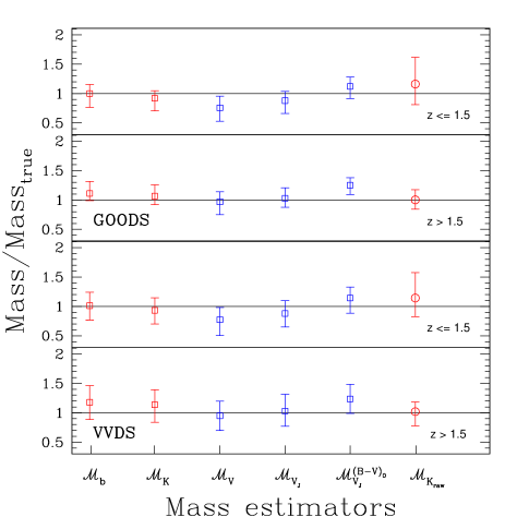
Figure 16: Retrieved mass values obtained by means of different estimators are reported normalized to their true values. Open points represent the median values of the ratio between the retrieved mass value and the true one, squares stand for mass estimates depending on the best fitting template while the circle stands for the only estimate that does not need any multi-wavelength data fitting (i.e. raw value, derived from eq. (9)). The errorbars represent the 16th (lower bar) and 84th (upper bar) percentiles of the distribution of the same ratios, that means that the 68% of the results lie within the errorbars. The upper two panels summarize the results obtained with the GOODS mock catalog, while the lower two one those obtained with the VVDS mock catalog. Results are presented for simulated galaxies at $z\leq 1.5$ (upper first and third panels) and at $z>1.5$.

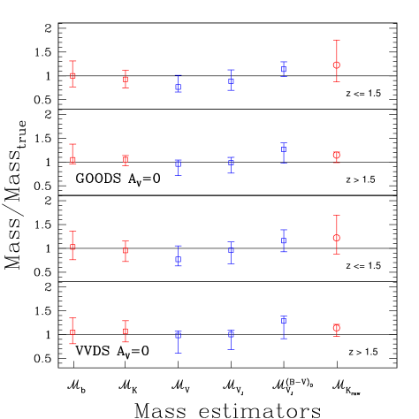
Figure 17: The same as in figure 16, but considering only simulated galaxies with A${}_{V}=0$ analyzed assuming no dust extinction.

Figure 16 and 17 summarize the results obtained for the sample of simulated galaxies when dust is a free unknown parameter and when extinction effects are excluded, respectively. Open points represent the median value of the ratio between the retrieved mass content and the true one, and they represent the trend of each mass estimator to well reproduce the true stellar mass content of galaxies or to over or under estimate it. The errorbars represent the 16th (lower bar) and 84th (upper bar) percentiles of the distribution of the ratios between retrieved and true values of stellar mass content, that means that the 68% of the values lie within the errorbars. The comparison between the upper two panels with the lower two ones allows to appreciate the influence of the photometric errors in the mass estimates obtained with the reported estimators. The comparison between results reported in the first and third upper panels ($z\leq 1.5$) with those reported in the second and fourth lower panels ($z>1.5$) allows to understand the behaviour of each mass estimator when different ranges of age are considered, because at $z>1.5$ the stars populating the galaxies are forced to be younger the 2 Gyr. Finally, the comparison between the results reported in figure 16 with the corresponding ones reported in figure 17 allows to understand the role of the lack of knowledge of the dust extinction affecting the luminosities of the galaxies when deriving their stellar masses.

4.2.1 $\mathcal{M}_{b}$

The best mass estimates can be derived by $\mathcal{M}$_b that retrieves values between 0.7 and 1.2 (0.5 and 1.5) of the true ones for 68% (100%) of the simulated galaxies for both the VVDS mock catalog and the GOODS one at $z\leq 1.5$. Simulated galaxies in the VVDS mock catalog at $z>1.5$ (i.e., with large photometric errors for the fainter galaxies) still obtain the correct estimate within 0.8 and 1.5 (0.5 and 2.0) with this estimator. Another advantage in using $\mathcal{M}$_b as mass estimator is that the probability of an overestimate of the true mass content of galaxies is the same of its underestimate. Indeed the median values of the distribution of $\mathcal{M}$_b/$\mathcal{M}$_true is 1 within 0.07, and only for galaxies with large photometric errors it becomes larger than 1 (e.g. for the VVDS simulated galaxies at $z>1.5$ is 1.18, while for the GOODS ones at $z>1.5$ is 1.11). Figure 17 reveals that the reason of this overestimate of the mass content is related to the possible overestimate of the dust extinction. Indeed, when this effect is removed, even the faintest galaxies obtain on average the correct estimate of their mass content by means of $\mathcal{M}$_b.

4.2.2 $\mathcal{M}_{K}$

Another good mass estimator is $\mathcal{M}$_K that displays an uncertainty similar to that of $\mathcal{M}$_b, that is it retrieves the correct value of the mass content within 0.7 and 1.2 (0.5 and 1.5) for 68% (100%) of the simulated samples at least at $z\leq 1.5$. For the faintest objects, like those in the VVDS mock catalog at $z>1.5$, $\mathcal{M}$_K is even more precise than $\mathcal{M}$_b when considering the whole range of results. On the other hand, $\mathcal{M}$_K displays a trend to slightly underestimate the true mass content of galaxies, and the median value of $\mathcal{M}$_K/$\mathcal{M}$_true is 0.9 for $z\leq 1.5$ galaxies and it becomes 1.0 only for the youngest ones ($z>1.5$) at least in the GOODS mock catalog where photometric errors are smaller. The same effect is appreciable in figure 17 that means that it is not due to wrong dust extinction estimate. The fact that the underestimate of the mass content is found only for galaxies at $z\leq 1.5$ reveals that the problem is related to the age estimate of the galaxies, that at lower redshift, where a larger range of acceptable ages is allowed, is slightly underestimated on average. Lower ages means lower $\mathcal{M/L}$ ratios as well shown in Appendix A. Indeed, we verified a median difference between the retrieved ages and the true ones of 0.3 Gyr for $z\leq 1.5$ while it is 0.0 at higher redshift.

4.2.3 $\mathcal{M}$ from V band estimators: $\mathcal{M}$_V, $\mathcal{M}$${}_{V_{J}}$ and $\mathcal{M}$${}_{V}^{(B-V)_{0}}$

A general trend to underestimate the mass content of galaxies is displayed by the mass estimator $\mathcal{M}$_V, that retrieves on average a value of mass that is only 75% of the true one. The underestimate is less evident at $z>1.5$ (where ages are better estimated) but it is still appreciable ($\mathcal{M}$_V is 90% of the true mass content). The reason of this trend is not related only to the possible wrong dust extinction estimate because it is confirmed even in figure 17 where dust effects are excluded. Indeed, a large part of this effect is caused by the underestimate of the V band luminosity by means of M_V (see figure 15). The luminosity underestimate, that is of 0.1 mag on average, leads to underestimate the mass content to about 0.9 of its true value, that matches the underestimate found at $z>1.5$. When $z\leq 1.5$ we have already mentioned for the K band that the underestimate of the age of the stellar populations produces the underestimate of the $\mathcal{M/L}$ ratio. In the V band the effect is even larger (see figure A1) and this explains the strong underestimate found at $z\leq 1.5$ in the mass value derived by means of $\mathcal{M}$_V. The mass estimates obtained by means of $\mathcal{M/L}$_V but which adopt the V band magnitude derived by the observed J band, $\mathcal{M}$${}_{V_{J}}$, do not suffer of the same problem of underestimate of $\mathcal{M}$_V, and they are closer to the correct values. At $z>1.5$ $\mathcal{M}$${}_{V_{J}}$ retrieves the correct value of the mass content of 68% (100%) of the galaxies within 0.8-1.2 (0.5-1.5) for the GOODS mock catalog and within 0.7-1.3 (0.4-1.6) for the larger errors of the VVDS mock catalog. At $z\leq 1.5$ $\mathcal{M/L}$_V still underestimates the true $\mathcal{M/L}$ ratio in the V band because of the underestimates of the ages, and $\mathcal{M}$${}_{V_{J}}$ is on average 85% of the true value. The use of $\mathcal{M/L}$${}_{V}^{(B-V)_{0}}$ instead of $\mathcal{M/L}$_V makes the mass obtained by means of $\mathcal{M}$${}_{V}^{(B-V)_{0}}$ overestimated with respect to the true value, being around 1.3 for galaxies at $z\leq 1.5$ and 1.2 for galaxies at higher redshift. On the other hand, the 16th and 84th percentiles for this mass estimator are close to the median value at least as those of the the previous ones. Since Bell et al. (2005) have calibrated their $\mathcal{M/L}$ estimator on a sample of star forming galaxies, we believe that the same calibration is not valid for quiescent galaxies. Indeed, our results demonstrate that the possible powerful mass estimator $\mathcal{M/L}$${}^{(B-V)_{0}}_{V}$ should be used only in the studies of young/star forming galaxies at low redshift, while its use in different context could bring large errors and a general trend to strongly overestimate the stellar mass of galaxies.

4.2.4 $\mathcal{M}$_Kraw

The last mass estimator presented in figures 16 and 17 has the advantage that it can be used without the need of any fitting, that is without a good photometry needed to apply the best fitting technique. At $z\leq 1.5$ $\mathcal{M}$_Kraw retrieves masses which are around 1.25 of the true values, and 68% (100%) of the galaxies obtain stellar mass estimates within 0.9-1.8 (0.5-2.4) for both the two mock catalogs, a much worse result than that obtained with the other estimators. On the contrary, at $z>1.5$ $\mathcal{M}$_Kraw supplies values which have more or less the same confidence of the best mass estimators such as $\mathcal{M}$_b. Indeed, $\mathcal{M}$_Kraw at $z>1.5$ retrieves on average the correct value of the mass content of galaxies, and 68% (100%) of them obtain estimates within 0.8-1.2 (0.6-1.6). The reason of the bad results achieved at lower redshift is that at $z\leq 1.5$ the fit expressed in equation (11) on which the estimator $\mathcal{M}$_Kraw is based takes into account only old ages (i.e. ages older than 2.7 Gyr), while the simulated galaxies include also young (e.g. 1.7 Gyr old) galaxies which have a lower $\mathcal{M/L}$ ratio.

Summarizing, when photometric data are used to find the best fitting templates reproducing the observed early-type galaxies, the best mass estimate, not affected by any systematic trend, is that derived by the scaling factor between templates and data on average. Alternatively, the near-IR bands can be safely used to derive the mass content of early-type galaxies, while optical bands produces much larger uncertainties and general underestimate of the stellar masses which are difficult to be taken into account.

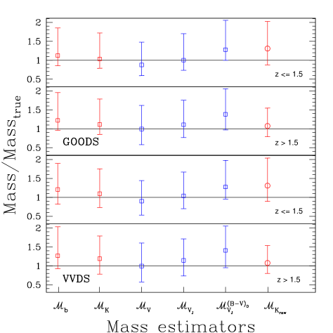
Figure 18: The same as in figure 16, but results are derived from mock catalogs built on the basis of an enlarged set of metallicities and of model codes (i.e. PEGASE, MA05 and GRASIL, see details in §4.2.4).

It is worth to note that all the comparisons made in this subsection are based on a fixed and known IMF (i.e. Salpeter IMF), and thus the uncertainties reported do not include the large uncertainty due to the lack of knowledge of the real IMF that produces real SEDs. At the same time, as we have seen in §3.2, IMFs can in many cases be considered scaling factors of the total stellar content at fixed luminosities. Anyhow, reported uncertainties for the mass estimates and for the luminosities are surely underestimated with respect to real data analysis also for another reason. Indeed, in the above test observations are simulated with templates that are contained in the spectral set used to analyze data, while in the reality synthetic templates are only approximation of the properties of real galaxies.

In order to take into account this point, we built an other set of simulated galaxies on the basis of templates including different metallicities and of the other codes listed in §2.2 (i.e., PEGASE, Ma05, GRASIL). All the galaxies are modeled assuming Salpeter IMF and following the combinations of ages and redshift already described at the beginning of this section. We used this new enlarged set of early-type galaxies models at $1<z<2$ to build new mock photometric catalogs, assuming again the uncertainties of the GOODS and VVDS surveys. The analysis of these new mock catalogs has been performed in the same way as the previously built ones. In particular, we continued to adopt a set of templates at solar metallicity and based on the BC03 code for the comparison in hyperz. The results are presented in figure 18, and they can be directly compared with those in figure 16. As anticipated, errorbars (16th and 84th percentiles of the distribution of the ratio $\mathcal{M}$_retrieved/$\mathcal{M}$_true) are larger in figure 18 than in figure 16, and their width is almost the same (i.e. $\sim$0.7-0.8) for all the mass estimators presented. From figure 18 it can be deduced that even at fixed and known IMF, the mass content of the early-type galaxies at $1.0<z<2.0$ can be retrieved within 0.7-1.5 (0.4-3.0) of the true value for 68% (100%) of the simulated sample, that is not better than a factor 2-3.

4.3 Different codes, different results?

In this section we quantify the differences in the stellar mass estimates obtained by means of the best fitting of the spectrophotometric data of 10 real early-type galaxies at $1<z<2$. The mass estimators described in the previous section are used to calculate the stellar content of 10 massive early-type galaxies at $z\simeq 1.5$ using hyperz to fit their spectrophotometric data.

The sample of 10 massive galaxies is described in a series of papers (i.e., Saracco et al. 2003; Saracco et al. 2005; Longhetti et al. 2005). The optical (B, V, R, I) and near IR (J and K’) magnitudes of the galaxies in the sample are from the Munich Near-IR Cluster Survey (MUNICS; Drory et al. 2001). In the best fitting procedure we also include further 5 points derived from the observed spectra, four in the wavelength range $0.9<\lambda<1.2$ $\mu$m and one in the H-band (see details in Saracco et al. 2005). The best fitting procedure follows the original one described in Saracco et al. (2005) and Longhetti et al. (2005), but four different set of templates are here adopted. We refer to the “BC03 set” as the one based on the BC03 code, including four SF histories ($\tau=0.1,0.4,0.6,1.0$ Gyrs) and four values of the stellar metallicity ($Z_{\odot}$, 0.2$Z_{\odot}$, 0.4$Z_{\odot}$, and 2.5$Z_{\odot}$). The “Ma05 set” is composed by templates built with the Ma05 code with fixed solar metallicity and with three SF histories ($\tau=0.1,0.4,1.0$ Gyrs). The “PEGASE set” includes the same four SF histories as the BC03 one, but the metallicity within each model is not fixed and it depends on the age of the template selected. Finally, the “Grasil set” is composed by only one SF history, described in §2.2, with stellar metallicity that increases with time following a chemical evolution prescription as in the case of the PEGASE set. All the four sets of models have been built with the Salpeter IMF to make easy comparisons among the different results obtained with the different codes.

If we consider the best fit for each galaxy, mass estimates obtained with the Ma05 set and with each of the estimators previously described are on average $0.8\pm 0.2$ with respect to the corresponding ones found with the BC03 set. Recent works on mass estimates which compare results based on different set of templates claimed that masses derived with the Ma05 set can be between 0.4 and 0.6 of the masses derived with the BC03 set (Cimatti et al. 2008). Indeed, the two apparently different findings are not surprising, since the above analysis is based on a sample of galaxies at $z\simeq 1.4$, which are on average older (i.e. ages $>1-2$ Gyr) than those contained in the comparison sample of Cimatti et al. (2008, $z>1.4$). Indeed, we checked (on the basis of simulated and not real galaxies) that at ages younger than few Gyr, mass estimates with the Ma05 templates are on average 0.6 of those derived with the BC03 ones.

The PEGASE set of templates supplies reasonable fits of the data only when dust is used as a varying parameter. Mass estimates obtained with PEGASE templates are on average larger (i.e. 1.1 and 1.3 with or without dust extinction respectively) than those obtained with the BC03 set of templates.

Finally, it is interesting to evaluate the results in the mass estimates that are achieved using the GRASIL code to build the set of templates used in the best fitting procedure. As already emphasized, the GRASIL code generates spectra of early-type galaxies following a self consistent picture of galaxy evolution, from the points of view both of star formation and of metal enrichment. Results are on average in very good agreement with those found with the BC03 set.

Summarizing, the use of different codes, at least those listed and discussed here, does not bring any significant change in the final results when stellar mass content of early-type galaxies is calculated by means of best fitting the spectrophotometric data. In particular, when masses are estimated by means of comparison with the BC03 set of templates, the obtained values are on average between 0.8-1.3 of those which could be obtained with the other sets here considered. On the other hand, the intrinsic uncertainty in the stellar mass estimate is larger than the former range, being between 0.5-1.5 even in the case of good quality data as those of GOODS (see §4.2), and further differences can be found when different mass estimators are adopted, as already outlined in the previous section.

5 A new empirical mass estimator

As seen in the previous section, stellar mass content of high redshift early-type galaxies cannot be estimated better than a factor between 2 and 3 on the basis of photometric data depending on the quality of the available photometric data and/or on the distance (i.e. apparent luminosity) of the galaxies. All the estimators presented above require the choice of a template reproducing the observed SED of the galaxies, on the basis of which the $\mathcal{M/L}$ ratio and/or the k-corrections needed to transform observed fluxes into stellar mass estimates are derived. In the following we present a new stellar mass estimator based uniquely on the apparent magnitudes in the K and V bands, and thus that it does not require any SED fitting. As for the other estimators, a requested a priori condition is that the redshift range of the galaxies is $1<z<2$ even if the correct redshift value can be poorly known (e.g. photometric redshift). As we will see, its precision is not lower than that of the other classic estimators, and in case of poor photometry it is more stable resulting even more reliable than the previous ones. On the other hand, with respect to the other classic estimators it presents the not negligible advantage that it does not require the fitting of large set of multi-wavelength photometric data.

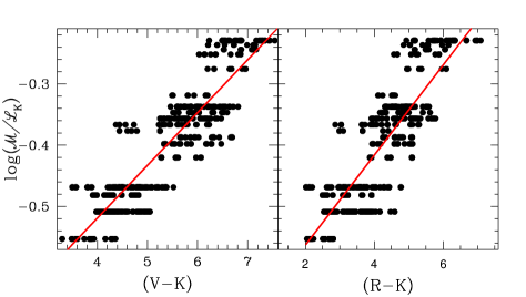
Figure 19: The $\mathcal{M/L}$_K ratio of the simulated galaxies is plotted versus the (V-K) apparent colour (left panel) and the (R-K) apparent colour (right panel). The grey (red) line displays the fit of the data in both the two panels.

The new estimator is defined by the following equations:

$$\log[\mathcal{M}^{(V-K)}]=\log(\mathcal{M/L}_{K})-0.4\cdot M_{K}+0.4\cdot M_{K}^{sun}$$ (14)

where

$0.4\cdot M_{K}^{sun}=1.364$

and

$$\log[\mathcal{M/L}_{K}^{(V-K)}]=0.086\times(V-K)_{obs}-0.863$$ (15)

while (V-K)_obs is the observed (V-K) colour and $M_{K}$ is derived in a raw way, without any dust correction and assuming as k-correction value the one calculated by means of equation (10b) assuming the coefficients in Table 3 of case i):

$M_{K}=m_{K}-d\_mod(z)-kcor(z)$

and

$kcor(z)=-0.32-0.65\cdot z-0.314\cdot z^{2}-0.0735\cdot z^{3}$

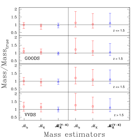
Figure 20: Results obtained with the new near-IR mass estimator $\mathcal{M}$${}_{K}^{(V-K)}$, defined on the basis of the K band luminosity derived in a raw way (i.e., without any dust correction and assuming as k-correction value the one calculated by means of equation (10b) assuming the coefficients in Table 3 of case i)) and on the $\mathcal{M/L}$ ratio that is a simple function of the apparent (V-K) colour: $\log(\mathcal{M/L}_{K})=0.086\times(V-K)_{obs}-0.863$. For comparison, we show also results obtained by means of $\mathcal{M}$_K and $\mathcal{M}$_b which contrary to $\mathcal{M}$${}_{K}^{(V-K)}$ require the fitting of the available multi-wavelength photometric data. Symbols and errorbars have the same meaning of those in figure 16. On the left, bars refer to results obtained on the mock catalogs built adopting solar metallicity and BC03 code, while on the right bars refer to the enlarged mock samples of galaxies simulated with different metallicities and different model codes (see text).

It is worthy to note that the equation defining the $\mathcal{M/L}$ ratio in the K band as a function of the (V-K) colour is totally empirical and it has been deduced by the observation that the apparent (V-K) colour follows a quite tight relation with $\mathcal{M/L}$_K for the model parameters representing the class of early-type galaxies (see §2). Figure 19 shows the relation between $\mathcal{M/L}$_K and the (V-K) colour (left panel). Points represent the simulated galaxies of the first set. The scatter of the relation expressed in eq. (15) is $\sigma=0.04$ and the maximum difference between the fit and the data of the simulated galaxies is $\pm 0.1$.

Figure 20 presents the results obtained with the new near-IR mass estimator $\mathcal{M}$${}_{K}^{(V-K)}$ (eq. 14 and 15), for the mock catalogs derived by the BC03 models at solar metallicity (third errorbars, left panels) and for the enlarged mock catalogs derived by means of a wide range of metallicities and of the other models listed in §2.2 (third errorbar, right panels). For comparison, we also show results obtained by means of $\mathcal{M}$_K and $\mathcal{M}$_b which contrary to $\mathcal{M}$${}_{K}^{(V-K)}$ require the fitting of the multi-wavelength photometric data. In spite of its simplicity, $\mathcal{M}$${}_{K}^{(V-K)}$ allows to obtain mass estimates even more precise than $\mathcal{M}$_b Indeed, the uncertainty introduced in the estimate of M_Kraw (see Fig. 15) combined with that of this new $\mathcal{M/L}$ estimator that retrieves $\mathcal{M/L}$_K within 0.9 and 1.1 (0.7 and 1.3) of the true values for 68% (100%) of the simulated sample, allows to obtain mass estimates between 0.8-1.1 for 68% of the simulated galaxies, to be compared with 0.7-1.4 of the $\mathcal{M}$_b estimator. Furthermore, $\mathcal{M}$${}_{K}^{(V-K)}$ is only slightly dependent on the photometric quality of the data. Indeed, results are similar for the VVDS and GOODS data set, while $\mathcal{M}$_K and $\mathcal{M}$_b show larger errors for the former sample with respect to the latter one. Finally, as it can be deduced from the last three errorbars in each panel of figure 19, $\mathcal{M}$${}_{K}^{(V-K)}$ retrieves the correct value of the stellar mass content within 0.8-1.7 for 68% of the galaxies even when simulated with a larger range of metallicities and of synthetic codes, to be compared with 0.8-2.0 of $\mathcal{M}$_b. Thus, recalling again that the calculation of $\mathcal{M}$^(V-K) does not require any fitting of large set of photometric data, we consider this mass estimator as the one to be recommended, in particular when poor photometry is available.

As an exercise, we applied this new estimator to the sample of early-type galaxies at $z>1$ presented by Saracco et al. (2008). We considered only galaxies for which V and K band magnitudes were available, for a total number of 15 galaxies at $1.2<z<1.9$ and apparent K band magnitudes between 16.6 and 19.8. Table 2 in Saracco et al. (2008) reports also their redshift and their stellar mass content derived by means of the $b$ best fitting parameter assuming the Chabrier IMF. We calculated for all these galaxies the stellar mass content by means of $\mathcal{M}$${}_{K}^{(V-K)}$ as defined above, and we further applied a multiplying factor of 0.55 to transform Salpeter based mass estimates into Chabrier based ones (see eq. 12). For 12 out of the 15 galaxies (80% of the sample), $\mathcal{M}$${}_{K}^{(V-K)}$ agrees with the values listed in Table 2 within a factor of 2, that is well within the intrinsic uncertainty of the mass estimate itself. For the remaining three galaxies the difference between the two estimates is larger (e.g. a factor 3) and it reaches a factor 5 in one case. Since we do not know which is the true value of the stellar mass of the analyzed galaxies, we can conclude that the classic estimators and our new estimator provide discrepant values in less than 15% of the cases.

Given its simplicity and its stability with respect to photometric inaccuracy/uncertainties, the mass estimator $\mathcal{M}$${}_{K}^{(V-K)}$ provides reliable and homogeneous mass estimates which can be easily compared among them since the dependence on models and on model parameters is cancelled. For these reasons, we believe that it should be adopted for all the samples of bona fide elliptical galaxies at $1<z<2$ which are the morphological type and the range of redshift for which the estimator has been tested. Obviously, the larger is the error in the redshift estimate the larger is the corresponding error in the mass estimate obtained with $\mathcal{M}$${}_{K}^{(V-K)}$, but the same is true of all the other estimators. An immediate application could be to the samples of EROs (e.g. (R-K)$>$5) for which a morphological information is available (e.g. HST images) and for which redshift can be deduced both on the basis of photometry and on the basis of spectral information.

Since the study of early-type galaxies is more often based on the (R-K) colour than on the (V-K) one, we tried to test the validity of a similar relation to obtain the K band mass to light ratio from (R-K). In the case of early-type galaxies simulated only with the BC03 models at solar metallicity, a linear relation between $\mathcal{M/L}$_K and the apparent (R-K) colour as

$$\log(\mathcal{M/L}_{K}^{(R-K)})=0.073\times(R-K)_{obs}-0.710$$ (16)

is not worse than the previous one between $\mathcal{M/L}$_K and the apparent (V-K) colour (see right panel of figure 19). Indeed the scatter of the relation expressed in eq. (16) is $\sigma=0.05$ and the maximum difference between the fit and the data is $\pm 0.13$. The problem arises when we consider galaxies modelled with other templates and with other metallicities. While the relation involving (V-K) remains stable and it continues to give good results, the one based on the (R-K) colour displays a much larger uncertainty. In other words, the apparent (R-K) colour of simulated early-type galaxies at $1<z<2$ is sensitive to the specific code and/or metallicity adopted to model the galaxies, while the (V-K) colour remains more constant over model details.

6 Summary and conclusions

The aim of the present paper is to quantify the dependence of the estimates of some basic properties of early-type galaxies, such as their luminosities and stellar masses, on the different models and model parameters which can be assumed to analyze the observational data. In other words, we want to answer to the question: do different model codes (and different model parameters assumed within the same code) produce significantly different results when they are used to derive luminosity and mass estimates of early-type galaxies?

In the first part of the paper, we analyzed the dependence of the $\mathcal{M/L}$ ratio and of the k-corrections for fixed age and z values from different model parameters (such as metallicity and IMF) and different model codes among some of the most popular ones: BC03, CB08, Ma05, PEGASE, GRASIL. We found that the best accuracy in the determination of both the two quantities is achieved in the near-IR bands. Furthermore, even if CB08 and Ma05 models give results different from the other codes when deriving $\mathcal{M/L}$_K and K band k-corrections, the combination of the same two quantities required to derive the stellar mass starting from the apparent K band magnitude is such that it results similar to that calculated with the other codes. In other words, the stellar mass estimate derived from the apparent K band magnitude assuming fixed IMF, at known age and z, is the same for all the models here considered within 20%. Equation (11) in §3.3 summerizes this finding by supplying the fit of $\log[$$\mathcal{M}$${}^{Sal}(z)]$ as function of $m_{K}$ and $z$. This fit allows to recover within 20% the stellar mass estimate that would have been recovered adopting all the models here considered for the same value of $z$ and $m_{K}$. Stellar masses derived assuming the Salpeter IMF can be transformed into those which would be obtained with Chabrier and Kroupa IMFs reducing them by a factor 0.55 and 0.62 respectively, without loosing precision beyond the limit of 20%. On the other hand, the proposed fit cannot be considered a reliable mass estimator given the a priori assumptions made to define it, such as the fixed solar metallicity, a fixed very simple star formation history, a fixed formation redshift that fixes a single possible age for the stellar populations of the galaxies at a given redshift.

The second part of our work is dedicated to quantify the differences which can result in the mass and luminosity estimates obtained by means of the best fitting technique applied to the photometric SEDs of early-type galaxies at $1<z<2$. The main difference with the previous part is due to the fact that age is not fixed a priori and the analysis of the observed galaxies consists just in the determination of those model parameters (such as age, star formation time scales, metallicity) which produce the template best fitting the photometric data. In order to asses the reliability of this technique in deriving the luminosity and stellar masses of galaxies, we applied it to a set of simulated galaxies for which the input properties were known. Mock photometric catalogs reproducing the wavelength coverage and photometric accuracy of two main current surveys (i.e. VVDS and GOODS) have been built on the basis of models of early-type galaxies at $1<z<2$ assuming BC03 code, solar metallicity and Salpeter IMF. Templates include also models of galaxies which experienced a secondary star forming episode considering different combinations of strengths and ages of the burst. Then, we applied the best fitting technique to the mock catalogs by means of hyperz and assuming the typical parameters used to analyze the early-type galaxies. Once a best fitting template has been associated to each simulated galaxy, we compared the results obtained in the luminosity and stellar mass content estimates with the true known input values. As far as the luminosities are concerned, we found that for the same goodness of the best fit selected to represent the observations, the uncertainties in the determination of the V absolute magnitude are much larger than in the K band. In other words, it is easier to obtain a good determination of near-IR absolute luminosities than optical ones. For what masses are concerned, we found that the goodness of the mass estimate is dependent on the mass estimator adopted to derive it. The best mass estimate, not affected by any systematic trend, is that derived by the scaling factor between templates and data on average, that retrieves the correct value within a factor two. Alternatively, the near-IR bands can be safely used to derive the mass content of early-type galaxies, while optical bands produce much larger uncertainties and average underestimates of the stellar masses which are difficult to be taken into account.

The uncertainties mentioned above refer to a favorable and not realistic situation in which the SEDs of the observed galaxies can be well reproduced by means of the templates used to find the best fitting model. Indeed, both model galaxies and fitting templates are derived by means of BC03 code at solar metallicity and assuming Salpeter IMF. In order to take into account the fact that synthetic templates are only approximation of the properties of real galaxies, we built an other set of simulated galaxies on the basis of templates including different metallicities and based on other codes considered in the present work (i.e. PEGASE, Ma05, GRASIL). All the galaxies are modeled assuming Salpeter IMF and following the same combinations of ages and redshift of the previous case. We used this new enlarged set of early-type galaxy models at $1<z<2$ to build new mock photometric catalogs, assuming again the uncertainties of the GOODS and VVDS surveys. The analysis of this new mock catalogs has been performed in the same way of the previously built ones. In particular, we continued to adopt a set of templates at solar metallicity and based on the BC03 code for the comparison in hyperz. We find that the true mass content of the galaxies cannot be retrieved better than within a factor of 3, being the only difference among the different estimators their trend to over or under estimate it on average.

As a final test useful to answer to the question weather different models based on different codes can bring significantly different results in the mass estimate of early-type galaxies, we applied the best fitting technique to a set of 10 massive early-type galaxies at $z\approx 1.5$ (Saracco et al. 2003; Saracco et al. 2005; Longhetti et al. 2005). We adopted 4 sets of templates built on the basis of the spectrophotometric codes BC03, Ma05, PEGASE and GRASIL, among which we separately found the one best fitting the observed photometric SED of the galaxies. We found that stellar mass estimates obtained with the Ma05 set of templates are on average $0.8\pm 0.2$ than those obtained with the BC03 set, while in case of young (i.e. $z>1.5$) galaxies the same ratio is 0.6. Stellar mass estimates obtained with the PEGASE set of templates are on average larger by a factor 1.1 than those obtained with the BC03 set of templates, while those obtained with the GRASIL set of templates result on average in agreement with those found with the BC03 set.

Summarizing, the use of different codes, at least those listed and discussed here, does not bring any significant change in the final results when stellar mass content of early-type galaxies are calculated by means of best fitting their spectrophotometric data. In particular, when masses are estimated by means of comparison with the BC03 set of templates, the obtained values are on average between 0.8-1.3 of those which could be obtained with the other sets of templates here considered. On the other hand, the intrinsic uncertainty in the stellar mass estimate is larger than the former range, being not better than a factor 3 as previously stated.

Finally, we proposed a new empirical mass estimator $\mathcal{M}$${}_{K}^{(V-K)}$ defined on the basis of a raw measure of the K band luminosity (M_Kraw) and of the $\mathcal{M/L}$ ratio in the K band calculated as simple function of the apparent (V-K) colour ($\mathcal{M/L}$${}_{K}^{(V-K)}$). Both the two involved quantities M_Kraw and $\mathcal{M/L}$${}_{K}^{(V-K)}$ do not need any multi-wavelength data fitting. Indeed, M_Kraw is the absolute K band magnitude derived as $m-d\_mod(z)-kcor_{raw}$, where $kcor_{raw}$ is the value calculated by means of the fitting functions supplied in the first part of the work and depending only on the value of $z$. The value of $\mathcal{M/L}$${}_{K}^{(V-K)}$ is obtained from the apparent (V-K) colour as:

$$\log(\mathcal{M/L}_{K}^{(V-K)})=0.086\times(V-K)_{obs}-0.863.$$

In spite of its simplicity, $\mathcal{M}$${}_{K}^{(V-K)}$ allows to obtain mass estimates even more precise than $\mathcal{M}$_b (i.e. within a factor 2-2.5). Furthermore, contrary to the mass estimators based on the fitting of photometric data, $\mathcal{M}$${}_{K}^{(V-K)}$ is only slightly dependent on the available photometric quality. Its simplicity and its stability with respect to photometric uncertainties make the new mass estimator $\mathcal{M}$${}_{K}^{(V-K)}$ useful to derive stellar mass estimates of samples of bona fide elliptical galaxies at $1<z<2$ (e.g., to the samples of EROs with morphological information). The main advantage in the use of $\mathcal{M}$${}_{K}^{(V-K)}$ as stellar mass estimator is its independence of models, because its calibrations has been proved over a wide range of models and model parameters. This allows to compare masses estimated on different samples in an umbiased way and with no need of any a priori correction or conversion among different reference models.

Appendix A Mass to light ratios from the best fitting technique

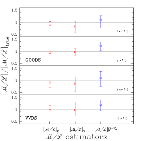
Figure 21: Retrieved mass to light ratios $\mathcal{M/L}$  in the K and V band are reported as normalized to their true values [$\mathcal{M/L}$]^true. Open square points represent the median values of the ratio between the retrieved mass value and the true one. The errorbars represent the 16th (lower bar) and 84th (upper bar) percentiles of the distribution of the same ratios, that means that the 68% of the results lie within the errorbars. The upper two panels summarize the results obtained with the GOODS mock catalog, while the lower two ones those obtained with the VVDS mock catalog. Results are presented for simulated galaxies at $z\leq 1.5$ (upper first and third panels) and at $z>1.5$.

In §4 we presented the results found by comparing the luminosity and mass estimates obtained by the best fitting technique with the known input values used to simulate some mock catalogs. Here, we briefly analyze the same comparison applied to the values of $\mathcal{M/L}$ ratios in both the K and V bands. We derive $\mathcal{M/L}$_K and $\mathcal{M/L}$_V which are the mass to light ratios corresponding to the best fitting template of each simulated galaxy. We also calculated $[\mathcal{M/L}_{V}]_{(B-V)_{0}}$ that is the mass to light ratio in the V band derived from the rest frame (B-V)₀ colour following the Bell et al. (2005) prescription:

$$log([\mathcal{M/L}_{V}]^{(B-V)_{0}})=-0.628+1.305(B-V)_{0}$$

The rest frame (B-V)₀ colour has been taken from the best fitting template of each galaxy.

In figure A1 the $\mathcal{M/L}$  ratios in the K and V band defined as detailed above are reported normalized to their true values. The retrieved values of $\mathcal{M/L}$_K are well within 0.7-1.1 (0.5-1.8) from the true values for 68% (100%) of the simulated galaxies. At lower redshift for both the two catalogs it can be noted a trend to underestimate the true value of $\mathcal{M/L}$_K by a factor of about 0.9, while at higher redshift (i.e. for the subsample of galaxies at only young ages) $\mathcal{M/L}$_K retrieves the correct value within 0.05. The underestimate of the $\mathcal{M/L}$ value in the V band and at $z\leq 1.5$ is even larger (i.e. around 0.8), and the uncertainties are much larger in this band than in the K band. Indeed, $\mathcal{M/L}$_V retrieves the correct value within 0.5-1.3 (0.2-2.4) for 68% (100%) of the simulated galaxies. The values of [$\mathcal{M/L}$_V]${}^{(B-V)_{0}}$ retrieved by means of the formula by Bell et al. (2005) show a smaller range of uncertainties with respect to $\mathcal{M/L}$_V obtained from the best fitting templates, but it displays a large trend to overestimate the true value of $\mathcal{M/L}$_V (i.e., by a factor 1.1-1.2).

References

- (1) Allen C. W., 1973, Astrophysical Quantities, Athlon Press, London
- (2) Alongi M., Bertelli G., Bressan A., Chiosi C., Fagotto F., Greggio L., Nasi E. 1993, A&AS 97,851
- (3) Bell E.F., Papovich C., Wolf C., et al. 2005, ApJ 625, 23
- (4) Bell E.F., Naab T., McIntosh D.H., et al. 2006, ApJ 640, 241
- (5) Bender R., Saglia R.P., Ziegler B., Belloni P., Greggio L., Hopp U., Bruzual G. 1998, ApJ 493, 529
- (6) Bolzonella M., Miralles J.-M. & Pellò R. 2000, A&A 363, 476
- (7) Bournaud F., Jog C. J. & Combes, F. 2007, A&A 476, 1179
- (8) Bressan A., Fagotto F., Bertelli G., Chiosi, C. 1993, A&AS 100, 647
- (9) Bruzual A.,G. & Charlot S. 2003, MNRAS 344, 1000 (BC03)
- (10) Calzetti D., Armus L., Bohlin R. C., Kinney A. L., Koorneef J., Storchi-Bergmann R. 2000, ApJ 533, 68
- (11) Cassisi S. & Salaris, M. 1997, MNRAS 285, 593
- (12) Cassisi S., degl’Innocenti S., Salaris, M. 1997, MNRAS 290, 515
- (13) Cassisi S., Castellani V., Ciarcelluti P., Piotto G., Zoccali M. 2000, MNRAS 315, 679
- (14) Chabrier G. 2003, PASP 115, 763
- (15) Charlot S. & Bruzual G. 2008, in preparation
- (16) Cimatti, A., Cassata P., Pozzetti L., et al. 2008, in press [astro-ph0001.1184]
- (17) Clegg R.E.S. & Middlemass D. 1987, MNRAS 228, 759
- (18) Daddi E., Renzini A., Pirzkal N., et al. 2005, ApJ, 626, 680
- (19) di Serego Alighieri S.,Vernet J., Cimatti A., et al. 2005, A&A, 442, 125
- (20) Elsner F., Feulner G. & Hopp U. 2008, A&A 477, 503
- (21) Faber, S.M. & Jackson R.E. 1976, ApJ 204, 668
- (22) Fagotto F., Bressan A., Bertelli G., Chiosi C. 1994a, A&AS 104, 365
- (23) Fagotto F., Bressan A., Bertelli G., Chiosi C. 1994b, A&AS 105, 29
- (24) Fioc, M & Rocca-Volmerange, B. 1997, A&A 326, 950 (PEGASE)
- (25) Girardi L., Bressan A., Chiosi C., Bertelli G., Nasi E. 1996, A&AS 117, 113
- (26) Grazian A., Fontana A., de Santis C., et al. 2006, A&A 449, 951
- (27) Groenewegen M.A.T. & de Jong T. 1993, A&A 267, 410
- (28) Kroupa P., 2001, MNRAS, 322, 231
- (29) Kurucz R.L. 1992, IAUS 149, 225
- (30) Lancon A. & Mouhcine M. 2002, A&A 393, 167
- (31) Le Fevre O., Guzzo L., Meneux B., et al. 2005, A&A 439, 845
- (32) Longhetti M., Saracco P., Severgnini P., et al. 2005, MNRAS 361, 897
- (33) Maraston C. 1998, MNRAS 300, 872
- (34) Maraston C. 2005, MNRAS 362, 799 (Ma05)
- (35) Maraston C., Daddi E., Renzini A., et al. 2006, ApJ 625, 85
- (36) Marigo P. & Girardi L. 2007, A&A 469, 239
- (37) McCarthy P.J., Le Borgne D., Crampton D., et al. 2004, ApJ 614, L9
- (38) Mignoli M., Cimatti A., Zamorani G., et al. 2005, A&A 437, 883
- (39) Rauch T. 2003, A&A 403, 709
- (40) Renzini A. 2006, ARA&A 44, 141
- (41) Rettura A. et al. 2006, A&A 458, 717
- (42) Salpeter E. E. 1955, ApJ 121, 161
- (43) Saracco P., Longhetti M., Severgnini P., et al. 2003, A&A 398, 127
- (44) Saracco P., Longhetti M., Severgnini P., et al. 2005, MNRASLet 357, 40
- (45) Saracco P., Longhetti M., Andreon S. 2008, MNRAS in press, arXiv:0810.2795
- (46) Shen S., Mo H.J., White S., Blanton M.R., Kauffmann G., Voges W., Brinkmann J., Csabai I. 2003, MNRAS 343, 978
- (47) Silva, L., Granato, G.L., Bressan, A., Danese, L., 1998, ApJ 509, 103 (GRASIL)
- (48) Thomas, D., Maraston, C., Bender, R., Mendes de Oliveira, C. 2005, ApJ 621, 673
- (49) Treu T., Ellis R.S., Liao T.X., al. 2005, ApJ, 633, 174
- (50) van der Wel A., Franx M., van Dokkum P. G., Rix H.-W. 2004 ApJ, 601, L5
- (51) van der Wel A., Franx M., van Dokkum P. G., Rix H.-W., Illingworth G. D. & Rosati, P. 2005, ApJ 631, 145
- (52) van Dokkum P. G., AJ 130, 2647
- (53) van Dokkum P. G., Franx M., Kelson D. D., Illingworth G. D., Fisher D., Fabricant D. 1998, ApJ 500, 714
- (54) Vanzella E., Cristiani S., Dickinson M., et al. 2008, A&A 478, 83
- (55) Vassiliadis E. & Wood P.R 1993, ApJ 413, 641
- (56) Ziegler B.L., Thomas D., Böhm A., Bender R., Fritz A., Maraston C. 2005, A&A 433, 519