Analysis and calibration of absorptive images of Bose-Einstein condensate at non-zero temperatures

Abstract

We describe the method allowing quantitative interpretation of absorptive images of mixtures of BEC and thermal atoms which reduces possible systematic errors associated with evaluation of the contribution of each fraction. By using known temperature dependence of the BEC fraction, the analysis allows precise calibration of the fitting results. The developed method is verified in two different measurements and compares well with theoretical calculations and with measurements performed by another group.

Submitted to: Rev. Sci. Inst.

I Introduction

Analysis of phase transitions offers valuable data of many physical systems. This is particularly true for studies of Bose-Einstein (BE) condensation in diluted gases Cor95 ; Ket95 . While such studies are very important scientifically, they pose many experimental challenges. The main difficulty is caused by extremely low temperatures in which Bose-Einstein condensates (BECs) are created and investigated, on the order of 100 nK. It is therefore essential to develop reliable detection/imaging methods for ultracold atoms close to the phase-transition point (density and temperature). Several such methods have been developed by many groups both destructive, like absorptive imaging, and nondestructive, like phase contrast Ket96 and polarization imaging Hul97 . The simplest and most often applied detection technique is the absorptive imaging and this is the method on which we concentrate in this paper.

In the absorptive imaging one records images of the shadow cast onto a camera sensor by atoms usually released from a trap during their free gravitational fall. This yields 2D distribution of optical density which reflects spatial density profile of the atomic cloud. Analysis of such profiles allows derivation of all relevant physical parameters of the investigated sample. The main difficulty in such analysis is associated with the fact that at finite temperatures the BEC fraction is always associated with some fraction of thermal (non-condensed) atoms. The thermal fraction plays a very important role in the data analysis as it allows determination of the cloud temperature. This fraction decreases with the falling temperature of the cloud. Each of the fractions has different density distribution and contributes differently to the recorded image. The coexistence and overlap of the two fractions results in a bimodal distribution of the optical density which raises interpretational problems. Below, we show that a simplistic analysis of such bimodal distributions by fitting them to a sum of the Gaussian and Thomas-Fermi functions corresponding to the thermal and condensate fractions, respectively, is not satisfactory and leads to systematic errors.

The problems associated with the analysis of absorption profiles are not new and were already noticed by several other groups Ket99 ; Cor96 ; KurnPhD . One attempt which partly avoids the problem of the bimodal distribution is the spatial separation of thermal and BEC fractions by the Bragg diffraction Kurn99 ; Ger04 or by application of an optical lattice Fer02 . These methods, however, are neither easy nor ideal as they also can introduce inter-fraction interaction. So far, the best known method is to analyze the thermal fraction only in its outer regions, outside the degenerate regime, where it is possible to use a simple classical description Ket99 . The main disadvantage of this method is that it is not easy and rather arbitrary to find the correct size of the excluded central region. As this region is enlarged, the systematic error of the fitted parameters is reduced, but the S/N ratio decreases. On the other hand, if the excluded central region is too small, the fit is performed to the data which sample also the edges of the degenerate region. The resulting systematic errors can be minimized, for example by applying corrections based on a numerical solution of the ideal Bose-Einstein distribution Cor96 , which is not a trivial task.

The present paper introduces the method allowing quantitative analysis of the absorptive pictures which ensures correctness of the size of the excluded degenerated region. We present the algorithm for analysis of the bimodal distributions which yields accurate ratio of the BEC and thermal fractions at finite temperatures. The analysis allows calibration of the thermal fraction fits and minimizes number of measurements necessary to obtain statistically meaningful averages.

Section II presents the procedure of fitting the bimodal distribution of optical density and the method for the fit optimization. In Section III we compare our method with other commonly used approaches. In Section IV we present examples of analysis of the experimental data with the two methods, the simplest one which uses a sum of a Gaussian and Thomas-Fermi distributions and the one we have developed. The paper is concluded in Section V.

II Method for analyzing the images of a condensate in non-zero temperature

This Section describes the main points of our method for analyzing the BEC pictures and its calibration.

II.1 Fitting to the bimodal distribution

Two-dimensional picture of a column optical density (OD) contains information on the spatial distribution of the column atomic density in a cloud $\tilde{n}\left(r,z\right)=OD\left(r,z\right)/\sigma_{0}$, where $r,z$ are the radial and axial coordinates, respectively, (Fig. 1) and $\sigma_{0}=3\lambda^{2}/2\pi$ is the normalized cross-section for atomic absorption at wavelength $\lambda$. By column densities we understand regular densities integrated over the local sample thickness, i.e. the column length. From the OD distribution recorded with light intensity $I$, the non-saturated distribution $OD_{n}$ can be calculated as $OD_{n}=OD+\left(1-\exp(-OD)\right)I/I_{sat}$, where $I_{sat}$ is the saturation intensity for the imaging transition. If the expansion of the cloud is small, we have to take into account that the cloud can be completely dark for the absorption probe beam (see, e.g. Lew03 ).

Well above the critical temperature, the density distribution in the thermal cloud can be described with the classical Boltzmann distribution. The column density is described then by the Gaussian function:

$$OD_{Gauss}(r,z)=OD_{Gpeak}\ \mathrm{exp}\left[-\frac{1}{2}\left(\frac{r-r_{c}}{\sigma_{r}}\right)^{2}-\frac{1}{2}\left(\frac{z-z_{c}}{\sigma_{z}}\right)^{2}\right],$$ (1)

with $\sigma_{r},\sigma_{z}$ being the half-width of the atomic density distribution in the radial and axial directions, respectively, $OD_{Gpeak}$ denotes the maximum value of the thermal fraction density, and $(r_{c},z_{c})$ are spatial coordinates of the maximum. For temperatures close to and lower than the critical value, the density distribution becomes predominantly the Bose distribution. Then, if the chemical potential is set to zero, the column optical density can be described by the, so called, Bose-enhanced Gaussian function Ket99 ; KurnPhD :

$$OD_{EnhGauss}(r,z)=OD_{Gpeak}\frac{g_{2}\left[\mathrm{exp}\left[-\frac{1}{2}\left(\frac{r-r_{c}}{\sigma_{r}}\right)^{2}-\frac{1}{2}\left(\frac{z-z_{c}}{\sigma_{z}}\right)^{2}\right]\right]}{g_{2}(1)},$$ (2)

where $g_{2}\left(x\right)=\sum^{\infty}_{n=1}\left(x^{n}\right)/\left(n^{2}\right)$ (see, e.g. Hua87 ).

With increasing distance from the position of the maximum density, the series terms in numerator of (2) decrease to zero. At appropriate distance, function (2) becomes the Gauss function (1) which justifies description of the density distribution at the edges of the thermal fraction by function (1). Nevertheless, more accurate results are obtained if the first three terms of series (2) are used instead. Including of yet more terms only increases computation time without noticeably improving the accuracy.

In the BEC fraction, on the other hand, the distribution of the column optical density of atoms in the Thomas-Fermi regime can be described by the TF profile, a clipped parabola,

$$OD_{TF}(r,z)=OD_{TFpeak}\ \mathrm{max}\left[0,\left(1-\left(\frac{r-r_{c}}{R_{r}}\right)^{2}-\left(\frac{z-z_{c}}{R_{z}}\right)^{2}\right)^{3/2}\right],$$ (3)

where $R_{z},R_{r}$ are the TF radii in the radial and axial directions, respectively, and $OD_{TFpeak}$ denotes maximum of the condensate optical density. When a condensate is not in the TF regime, the density distribution is well approximated by a Gauss function Ket99 .

All pictures in our procedure are taken with the condensates that were expanding for time $t$ after their releasing from MT. Knowing spatial distribution of the atomic density in the falling cloud, the initial atomic temperature can be determined Ger04_t :

$$T=\frac{2\tau_{r}^{2}}{1+3\tau_{r}^{2}}T_{r}+\frac{1+\tau_{z}^{2}}{1+3\tau_{z}^{2}}T_{z},$$ (4)

where $\tau_{i}=\omega_{i}t$ for $i=z,r$ and $T_{i}=(m/2k_{B})\left[\omega_{i}^{2}\sigma_{i}^{2}(t)/(1+\omega_{i}^{2}t^{2})\right]$ are the effective temperatures measured after expansion. Moreover, the distribution allows determination of the numbers of atoms in each fraction, the thermal fraction $N_{th}$ and the condensate fraction $N_{BEC}$:

$$N_{th}=\left(2\pi\right)^{3/2}\frac{OD_{Gpeak}}{\sigma_{0}}\sigma_{r}^{2}(t)\sigma_{z}(t),$$ (5)

$$N_{BEC}=\frac{8}{15}\pi\frac{OD_{TFpeak}}{\sigma_{0}}R_{r}^{2}(t)R_{z}(t).$$ (6)

The values of the distribution parameters are to be derived by fitting the $OD$ distribution functions to the experimentally recorded profiles. For pictures corresponding to homogenous samples consisting exclusively of either thermal atoms or pure BEC, the functions (1), (2) or (3) can be fitted, as appropriate. Such fits are performed for the radial and axial sections independently. The sections cross the center of mass which coincides with the maximum of optical density. In the least-squares fitting procedure the MINUIT library minuit was used.

In a bimodal atom cloud, containing both the BEC and thermal fractions, the recorded pictures consist of two regions, the external region occupied by the thermal cloud only and the internal one where the two fractions coexist. In the later region and close to the border between the two regions the density distribution is distorted by the interaction between the fractions and by the Bose enhancement of the thermal fraction Ket99 ; KurnPhD . To reduce the effect of this distortion, the fitting has to be performed in several steps.

The first step is to determine the region occupied by the condensate and its direct neighborhood. For this sake, we approximate the bimodal distribution by the sum of functions (1) and (3) with some offset and fit it to the column density picture of the atomic cloud. The fit is performed for each direction independently with the least-squares fitting procedure based on the MINUIT library.

Next, using the parameters derived from the fitting curve (3), the initial BEC extension, i.e. the TF radii, $R_{z},R_{r}$, are determined. This allows to subtract the BEC contribution from the analyzed picture. To account for distortions in the intermediate region, the size of the subtracted area is taken with some margin such that the area dimensions are bigger than $R_{z}$ and $R_{r}$ by scaling factor $S$ (see Fig. 1). The procedure of exact determination of the $S$ value is described in the following subsection.

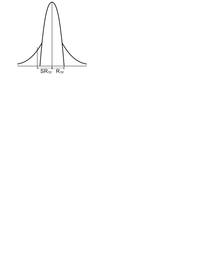
Figure 1: Illustration of the spatial extension of the thermal (outer) and BEC (central) fractions fitted by different distributions. The scaling factor $S$ is chosen for each picture individually to account for the distortion of the density distribution in the intermediate region, as described in Subsec. II.2

.

After removing the BEC contribution with appropriate safety margins determined by the scaling factor, the remaining image consists already of a pure thermal fraction and can be fitted by first three terms of series (2) with some background. We do it with the least-squares method by the 2D NonLinearFit function in Mathematica 5.1. The fit parameters allow calculation of the atom number in a thermal cloud and its temperature.

Having determined the optical density distribution in the thermal fraction and the background level, they can be subtracted from the initial picture with full bimodal distribution. Additionally, at this stage data points which are below 5% threshold are rejected to eliminate the contribution of the intermediate, distorted region of the cloud picture.

To such evaluated data the TF profile (3) is fit by the 2D least-squares method, which yields atom number in the BEC fraction and the appropriate TF radii. For minimization of $\chi^{2}$, the NMinimize function in Mathematica is used.

II.2 Calibration of the thermal fraction region

The value of coefficient $S$ affects the calculated temperature and atom number of the BEC fraction in a bimodal distribution. Taking too big margin, i.e. too big $S$, eliminates too large region which contains information on the density distribution of the thermal fraction, thereby lowering the signal/noise ratio and reducing the fit accuracy. Too small value of $S$, on the other hand, introduces systematic errors by including the distorted regions.

Fig. 2 illustrates the effect of the value of scaling factor $S$ on the calculated temperature of the bimodal cloud in the radial and axial directions. All fits used for this figure were performed for the same picture of a thermal condensate. Fig. 2 illustrates that there exists a fairly wide range of the $S$ values where the determined temperature does not change by more than one standard deviation (shaded range in Fig. 2). For $S<1$, the determined temperature is underestimated by including the intermediate border region affected by the BEC fraction, while for $S>1.8$, the temperature is not correctly estimated because of low S/N ratio of a too much reduced picture. The choice of appropriate value of $S$ requires taking into account also the effect of $S$ on the number of atoms in the BEC fraction derived from the fit. This effect can be seen when studying the phase-transition plot, i.e. the dependence of the BEC size normalized to all atoms in a bimodal cloud, $N_{0}/N=N_{BEC}/(N_{BEC}+N_{th})$, on the reduced temperature $T/T_{C}(N)$ with $T_{C}(N)=\hbar/k_{B}\left[N\cdot(\omega_{r}^{2}\omega_{z}/1.202)\right]^{1/3}$ being the critical temperature.

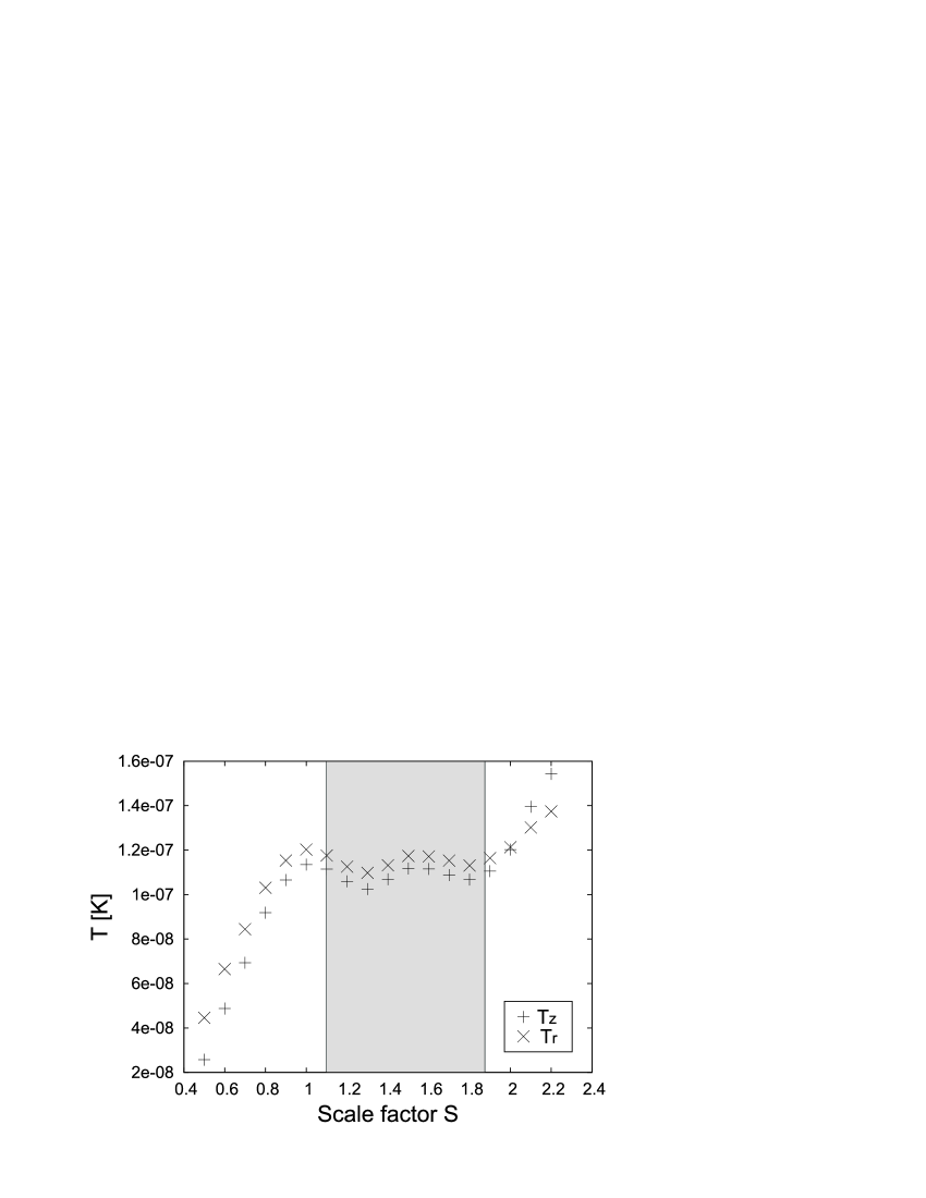
Figure 2: Temperature values in the radial and axial directions determined for experimental recording analyzed with different values of $S$. The marked region indicates the range of $S$ values for which the determined temperature does not change by more than one standard deviation.

Figure 3: Condensate fraction versus normalized temperature. The points represent results of fitting the bimodal distributions obtained with different values of scaling parameter S (between 0.8 and 1.8) to four different images (marked by different symbols: $\diamondsuit,\bigcirc,+$, and $\times$), as described in text. The elliptical contours depict the regions of concentration points, i.e. those where the derived values of atom number and reduced temperature weakly depend on $S$. The solid line represents function $N_{0}/N=1-(T/T_{C}(N))^{3}$ Gro50 and the broken line represents behavior of a trapped, semi-ideal Bose gas Nar98 .

Nonetheless, the check that the measured temperature of the cloud is independent of the size of the exclusion region is not the sufficient criterion of the fit quality. Particularly, if the measured data is heavily affected by noise or if the image sizes of either fraction are comparable with the image resolution, the temperature stability region (shaded area in Fig. 2) can be very narrow or even vanish completely. We have, therefore, studied further consequences of various choices of the $S$ values.

In Fig. 3 we depict number of atoms in the BEC fraction versus the reduced temperature for four typical images of the bimodal cloud. Bimodal distributions corresponding to different values of $S$ were fitted to each of the pictures as described above (Subsec. II.1). For each recorded image the fitting procedure was performed for different values of $S$ which were increasing by constant increments from 0.8 to 1.8. For a specific range of $S$ the derived atom numbers, as well as the temperatures, concentrate around specific values, the ”concentration points”. They change very little with $S$ by no more than $\pm 5$%. This fact indicates that $S$ values within the given range provide optimal separation of the perturbed thermal fraction form the non-perturbed one which allows proper description of the thermal cloud by function (1) without sacrificing the S/N ratio too much.

A very convincing verification of the fit quality is the position of the ”concentration points” on the phase transition plots relative theoretical curves, like in Fig. 3 Gro50 ; Nar98 . If a given ”concentration point” appears far from the theoretical curve, it indicates that the corresponding image was too much affected by some nonstatistical noise, e.g. caused by interference fringes or systematics. In such case, another fitting should be tried with another (bigger or smaller) background around the atomic cloud. Our experience shows that in about 90% of all cases a single repetition of the fitting procedure yields a good result. The remaining 10% is most often associated with systematic errors.

Interference fringes can be removed to a large extent from the image by a sequential subjecting the data to FFT, the mask corresponding to the fringe frequencies and to reverse-FFT. This can be done, e.g. with the ImageJ software fringes . Examples of the heavy fringed and defringed images are presented in Fig. 4.

Under conditions of our experiment, the optimum $S$ values are between $1.1$ and $1.4$ and depend on the size of the BEC fraction. The center of the ”concentration point” on the phase transition plots gives the correct value of S, i.e. the correct size of the excluded degenerated region, while the size of the ”concentration point” allows to estimate its statistical uncertainty.

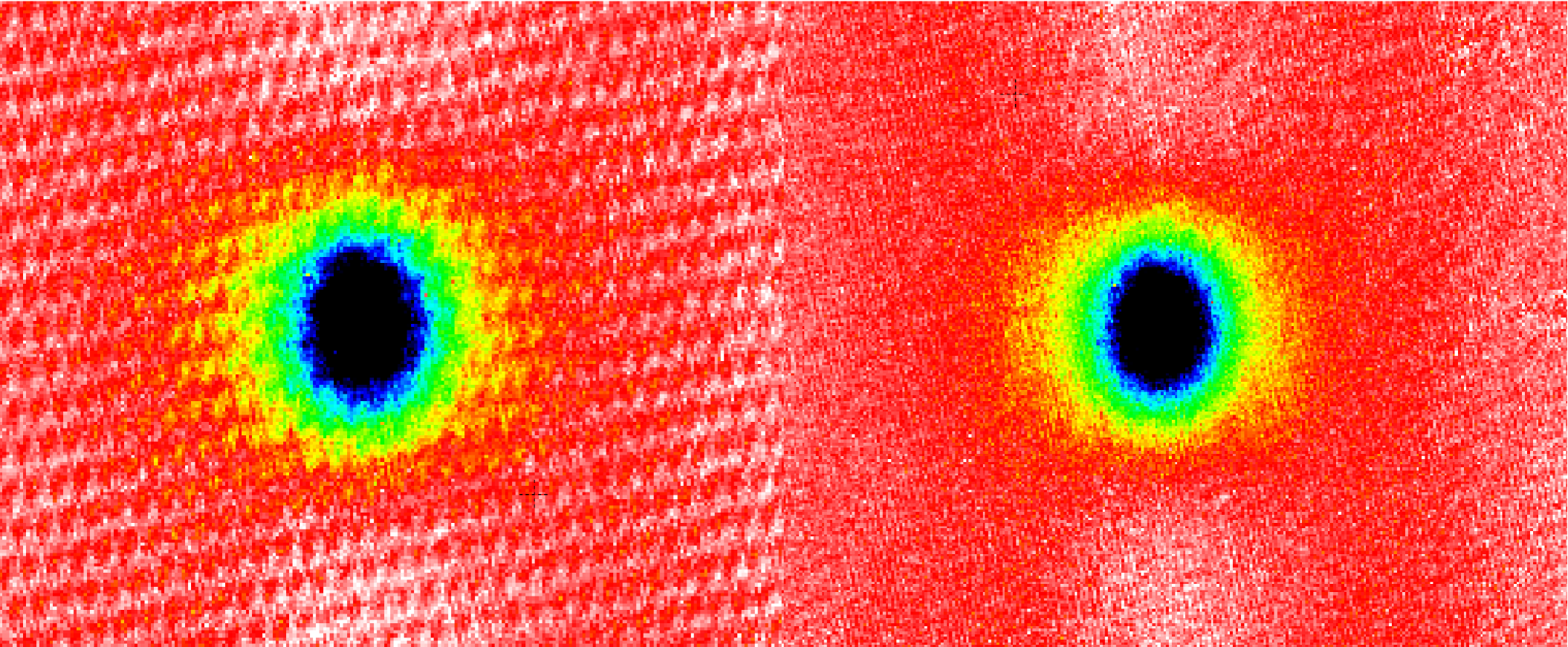
Figure 4: Examples of the heavily fringed and defringed images. The interference fringes have been removed from the original image as described in text.

III Comparison to other methods

In order to compare our method with the other approaches we have analyzed a condensate image created by a computer simulation. The simulation created a 2D atomic density distribution of a bimodal cloud with 0.4 BEC fraction in a given trapping potential. It was based on modelling of the BEC part by the Castin and Dum theory Cas96 , the thermal fraction by the Bose-enhanced distribution (2), and by taking into account their ballistic expansion within 22 ms. Finally, a noise typical for the recorded absorption pictures was added to such constructed simulation. In our simulation the thermal component is treated as an ideal Bose gas, while the condensate part is assumed to be in the TF regime.

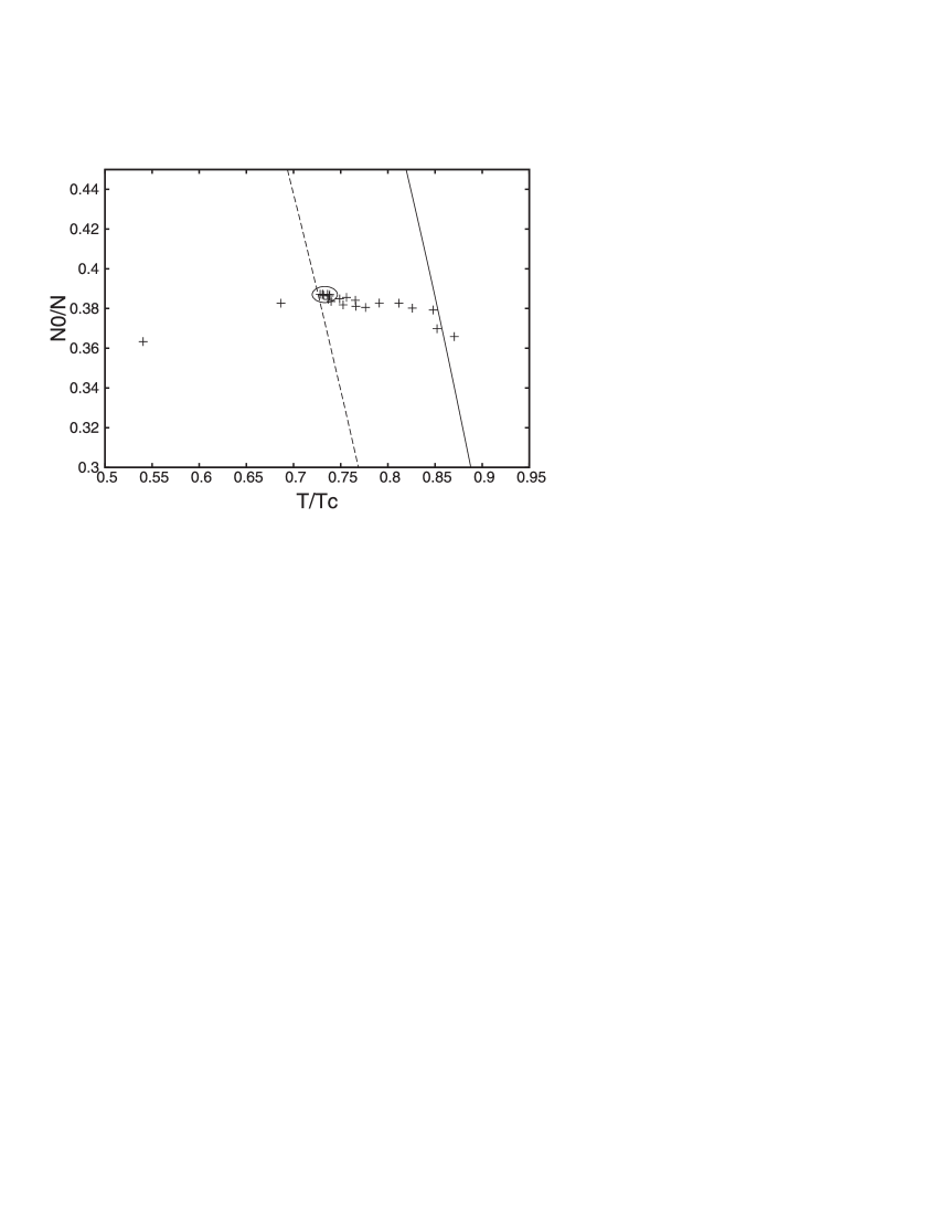
Figure 5: Expanded dependence of the condensate fraction versus normalized temperature. The points represent results of fitting the bimodal distributions to the image generated by simulation, as described in text, with the $S$ values in the range between 0.8 and 3.0. The elliptical contour marks the regions of concentration of nine points, where the derived values of the atom number and reduced temperature weakly depend on $S$. The solid line represents function $N_{0}/N=1-(T/T_{C}(N))^{3}$ Gro50 , the broken line represents behavior of a trapped, semi-ideal Bose gas Nar98 .

In Fig. 5 we depict the number of atoms in the BEC fraction versus the reduced temperature obtained by fitting the bimodal distributions to the image generated by the simulation. The $S$ values used in the fits are in the range between 0.8 and 3.0 with a step of 0.1. Similarly as in Fig. 3, the elliptical contour, indicates the regions of concentration of nine points, where the derived values of atom number and reduced temperature weakly depend on $S$.

The basic results of our analysis, i.e. the number of atoms in both the condensate $N_{0}$, and thermal $N_{th}$, components, temperature $T$ and the Thomas-Fermi radii $R_{z},R_{r},$ are compared with the values preset in the simulation and generated by other methods. The first method, due to its simplicity being probably the most common, fits a sum of the 2D Gaussian (1) and TF (3) distributions to the experimental data. In the second method the Gaussian function is fitted to the wings of the spatial distribution, then subtracted from the whole distribution and the remaining data is eventually fitted by the TF function. Fitting a 2D Gaussian to the wings of the distribution was widely used in the early experiments on BEC (e.g. Cor96 ; Kas99 ; Ing01 ; Gri02 ). The noise added to the simulated picture reproduces real experimental conditions and causes that neither of the methods gives the perfect fit. Still, the described method provides the the closest agreement with the simulation parameters.

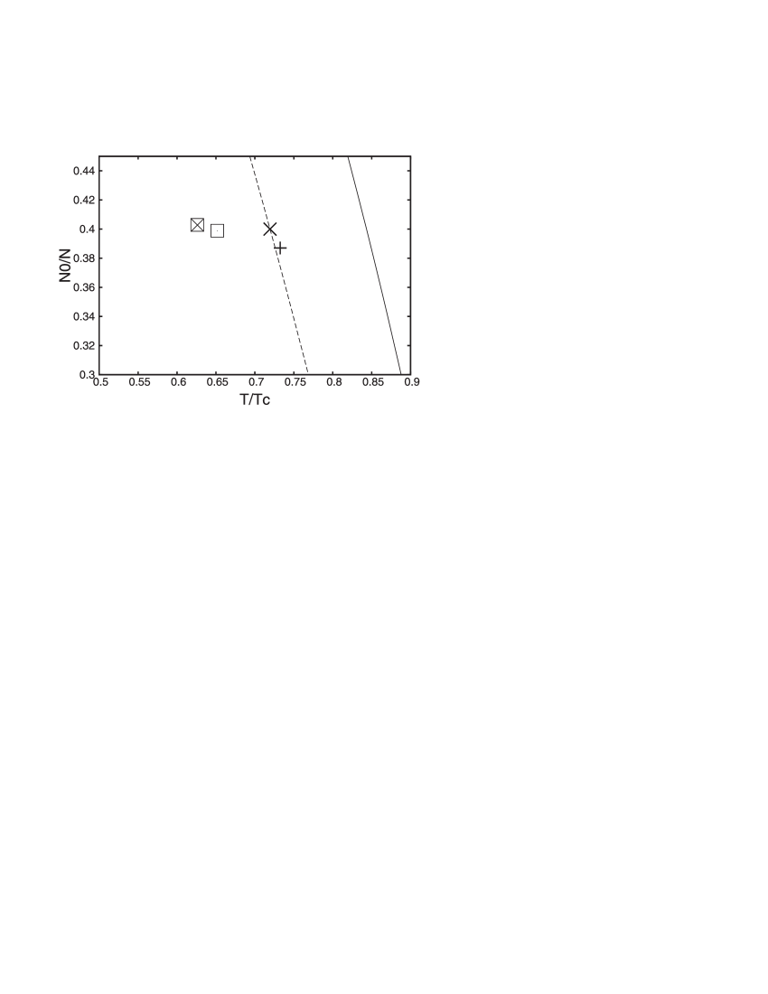
Figure 6: Condensate fraction versus normalized temperature - the results generated by different methods of image analysis applied to the simulated picture of a bimodal distribution. The value used in the simulation is depicted as $\times$. Our method gives the value represented by $+$, a simple 2D sum of the Gaussian and TF distributions gives $\boxtimes$, while a Gauss function used instead of the Bose-enhanced Gaussian gives $\boxdot$. The solid and broken lines have the same meaning as in Fig. 5.

	$N_{0}$	$N_{th}$	$T$	$R_{z}$	$R_{r}$
Simulation	1	1	1	1	1
Our method	1.0104	1.0660	1.0304	1.0045	0.995
2D SUM	1.0199	1.0082	0.8737	1.0081	0.995
GTF	1.0264	1.0310	0.9143	1.0084	0.996

Table 1: Results of the analysis of the simulated image by three different methods: our method, ”2D SUM” - the method with fitting a 2D sum of the Gaussian (1) and TF (3) distributions, ”GTF” - the fitting of the Gaussian function to the wings of the distribution and the TF function to the condensate part.

IV Typical examples

In this Section we discuss results of the analysis of the typical experimental images obtained with our setup Byl08 . The experiment was devoted to studies of the free-fall dynamics of a finite-temperature condensate of ⁸⁷Rb in the F=2 state and is described in more detail elsewhere Zaw08 . Here, we present two examples showing how the results derived with the method described in Sec. II compare with those obtained with the simple ”2D SUM” method based on summation of the Gauss and TF distributions. This comparison well illustrates the potential of our method.

IV.1 Dependence of $N_{0}/N$ on $T/T_{c}$

Fig. 7 represents a typical experimental dependence of the BEC fraction $N_{0}/N$ on the reduced temperature, $T/T_{C}$, analyzed with two approaches. The points represented in Fig. 7(a) are obtained by using the 2D fitting of the sum of functions (1) and (3) to the sections of absorptive images. The points in Fig. 7(b) are obtained using our fitting procedure (Sec. II). As before, the solid lines are the $N_{0}/N=1-(T/Tc(N))^{3}$ functions, while the broken ones represent results of the calculations along the lines of Ref. Nar98 . According to Ref. Ket99 , the bigger is the BEC fraction in the sample, the more the results of a simplistic fit with a sum of functions (1) and (3) deviate from the real temperature. The experimental data points are obtained from relatively small number of 210 BEC images taken at different temperatures. As can be seen in Fig. 7(b), experimental points evaluated with our method are in excellent agreement with the model of Ref. Nar98 , while those shown in Fig. 7 (a) deviate dramatically from theoretical predictions.

Figure 7: Comparison of the typical experimental dependences of the BEC fraction, $N_{0}/N,$ on the reduced temperature, $T/T_{C}(N),$ yielded by 210 images. The points in (a) result from simple fitting the 2D sum of functions (1) and (3) to the sections of absorption images, whereas the points in (b) correspond to the fitting procedure described in this paper. The solid and broken lines are the same as in Figs. 3, 5, and 6.

IV.2 Temperature dependence of the aspect ratio $R_{r}/R_{z}$ of a free falling BEC

Fig. 8 presents results of our measurements of the BEC aspect ratio as a function of the reduced temperature, $T/T_{C}$, evaluated from 150 images of BEC taken at different temperatures after $t=15$ ms free fall. As described previously, the data points in Fig. 8(a) were obtained by 2D fitting of a sum of functions (1) and (3) to the sections of absorptive images whereas those in Fig. 8(b) by using our new fitting method. The points evaluated with the new method behave qualitatively in the same way as in a similar experiment of Gerbier $et$ $al.$ Ger04 . However, in Ref. Ger04 the thermal and BEC fractions were completely separated spatially by Bragg diffraction which eliminated problems of their proper identification in the absorptive images. Despite different methods of the fraction separation, our method yields qualitatively similar results comparison . On the other hand, the points those obtained with the simple ”2D-SUM” method exhibit distinctly different, nonphysical behavior .

Figure 8: Comparison of the typical dependences of the BEC aspect ratio on the normalized temperature, $T/T_{C}$, obtained from 150 images taken after $t=15$ ms free fall. (a) depicts results of 2D fitting of a sum of functions (1) and (3) to the sections of absorption images, points in (b) are obtained by application of the described procedure.

V Conclusions

We have developed the method allowing proper interpretation of absorptive images of mixtures of BEC and thermal atoms which reduces possible systematic errors arising from non-Gaussian distribution of ultra-cold thermal atoms.

The developed algorithm is based on the fitting procedure of 2D density distributions to the absorption profiles describing the thermal fraction. By using the well known temperature dependence of the BEC fraction, the analysis allows precise calibration of the fitting results and, consequently, reduces number of measurements necessary to obtain statistically meaningful average values. We compare our method with the others commonly used. We have performed experiments verifying the developed method in two different measurements. Comparison of the results analyzed with our method and with the simplest fitting procedure demonstrates that the described method yields far better accuracy and is less prone to systematic errors. The results interpreted with our approach are also consistent with theoretical calculations and with the results of measurements performed by another group.

References

- (1) M.H. Anderson, J.R. Ensher, M.R. Matthews, C.E. Wieman, E.A. Cornell, ”Observation of Bose-Einstein Condensation in a Dilute Atomic Vapor,” Science 269, 198, (1995).
- (2) K.B. Davis, M.O. Mewes, M.R. Andrews, N.J. van Druten, D.S. Durfee, D.M. Kurn and W. Ketterle, ”Bose-Einstein Condensation in a Gas of Sodium Atoms,” Phys. Rev. Lett. 75, 3969, (1995).
- (3) M.R. Andrews, M.O. Mewes, N.J. van Druten, D.S. Durfee, D.M. Kurn and W. Ketterle, ”Direct, Nondestructive Observation of a Bose Condensate,” Science 273, 84, (1996).
- (4) C.C. Bradley, C.A. Sackett and R.G. Hulet, ”Bose-Einstein Condensation of Lithium: Observation of Limited Condensate Number,” Phys. Rev. Lett. 78, 985, (1997).
- (5) W. Ketterle, D. S. Durfee, and D. M. Stamper-Kurn, Proceedings of the International School of Physics ”Enrico Fermi”, Course CXL, edited by M. Inguscio, S. Stringari and C.E. Wieman (IOS Press, Amsterdam, 1999) pp. 67-176.
- (6) J.R. Ensher, D.S. Jin, M.R. Matthews, C.E. Wieman and E.A. Cornell, ”Bose-Einstein Condensation in a Dilute Gas: Measurement of Energy and Ground-State Occupation,” Phys. Rev. Lett. 77, 4984 (1996).
- (7) D.M. Stamper-Kurn, Peeking and poking at a new quantum fluid: Studies of gaseous Bose-Einstein condensates in magnetic and optical traps , PhD Thesis, Massachusetts Institute of Technology, (2000).
- (8) J. Stenger, S. Inouye, A.P. Chikkatur, D.M. Stamper-Kurn, D.E. Pritchard, W. Ketterle, ”Bragg Spectroscopy of a Bose-Einstein Condensate,” Phys. Rev. Lett. 82, 4569 (1999).
- (9) F. Gerbier, J. H. Thywissen, S. Richard, M. Hugbart, P. Bouyer, and A. Aspect, ”Experimental study of the thermodynamics of an interacting trapped Bose-Einstein condensed gas,” Phys. Rev. A 70, 013607 (2004).
- (10) F. Ferlaino, P. Maddaloni, S. Burger, F. S. Cataliotti, C. Fort, M. Modugno, and M. Inguscio, ”Dynamics of a Bose-Einstein condensate at finite temperature in an atom-optical coherence filter,” Phys Rev. A 66, 011604(R) (2002).
- (11) H. J. Lewandowski, D. M. Harber, D. L. Whitaker, and E. A. Cornell, ”Simplified System for Creating a Bose-Einstein Condensate”, J. Low Temp. Phys. 132, 309, (2003)
- (12) K. Huang, Statistical Mechanics, Second Edition, John Wiley and Sons, New York (1987).
- (13) F. Gerbier, J. H. Thywissen, S. Richard, M. Hugbart, P. Bouyer, and A. Aspect, ”Critical Temperature of a Trapped, Weakly Interacting Bose Gas,” Phys. Rev. Lett. 92, 030405 (2004).
- (14) F. James, MINUIT, Function Minimization and Error Analysis, Reference Manual Version 94.1, CERN Program Library Long Writeup D506, CERN, (1994)
- (15) S. R. de Groot, G. J. Hooyman, and C. A. ten Seldam, ”On the Bose-Einstein condensation,” Proc. R. Soc. London A 203, 266 (1950).
- (16) M. Naraschewski, D. M. Stamper-Kurn, ”Analytical description of a trapped semi-ideal Bose gas at finite temperature,” Phys. Rev. A 58, 2423 (1998).
- (17) M. D. Abramoff, P. J. Magelhaes, S. J. Ram, ”Image Processing with ImageJ,” Biophotonics International 11, 36, (2004)
- (18) Y. Castin and R. Dum, ”Bose-Einstein Condensates in Time Dependent Traps”, Phys. Rev. Lett. 77, 5315, (1996)
- (19) B. P. Anderson and M. A. Kasevich, ”Spatial observation of Bose-Einstein condensation of 87Rb in a confining potential”, Phys. Rev. A, 59, R938, (1999)
- (20) G. Modugno, G. Ferrari, G. Roati, R. J. Brecha, A. Simoni, M. Inguscio, ”Bose-Einstein Condensation of Potassium Atoms by Sympathetic Cooling”, Science, 294, 1320 (2001)
- (21) T Weber, J Herbig, M Mark, H -C Nägerl, and R Grimm, ”Bose-Einstein Condensation of Cesium”, Science Express, 10.1126/science.1079699, (2002).
- (22) F. Bylicki, W. Gawlik, W. Jastrzȩbski, A. Noga, J. Szczepkowski, M. Witkowski. J. Zachorowski, M. Zawada, ”Studies of the Hydrodynamic Properties of Bose-Einstein Condensate of 87Rb Atoms in a Magnetic Trap,” Acta Phys. Pol. A 113, 691 (2008).
- (23) M. Zawada, R. Abdoul, J. Chwedeńczuk, R. Gartman, J. Szczepkowski, Ł. Tracewski, M. Witkowski, W. Gawlik, ”Free-fall expansion of finite-temperature Bose-Einstein condensed gas in the non Thomas-Fermi regime”, accepted in J. Phys. B.; arXiv:0811.1672 (2008)
- (24) No quantitative comparison of the results of our work and that of ref. Ger04 is possible because of different conditions of the two experiments. In particular, in our case the free-fall time is ms, while in Ger04 it was ms. Also, our temperature is normalized to which depends on the total number of atoms , while in Ger04 the normalization was to the critical temperature of an ideal gas in a thermodynamic limit.