Large amplitude Love waves

Abstract

In the context of the finite elasticity theory we consider a model for compressible solids called “compressible neo-Hookean material”. We show how finite-amplitude inhomogeneous plane wave solutions and finite-amplitude unattenuated solutions can combine to form a finite-amplitude Love wave. We take a layer of finite thickness overlying a solid half-space, both made of different pre-stressed compressible neo-Hookean materials. We derive an exact solution of the equations of motion and boundary conditions, and also obtain results for the energy density and the energy flux of the waves. Finally, we investigate the special case when the interface between the layer and the substrate is in a principal plane of the pre-stain. A numerical example is given.

1 Introduction

A seismic event launches at least two types of surface waves, one causing vertical (elliptic) movements, the other causing rather destructive lateral (shear horizontal) movements. In the essay which won him the Adams Prize in 1911, Love [1] proposed a simple Earth model which supports the latter kind of waves, by considering a crust made of an isotropic, linear, elastic solid, rigidly bonded onto a substrate (a semi-infinite solid) made of another isotropic, linear, elastic solid. In this heterogeneous structure, a shear horizontal wave may propagate, leaving the upper face of the layer free of traction, and having an amplitude which decays rapidly with depth in the substrate. This localisation of the amplitude variation is what makes Love waves (and surface waves in general) a subject of great interest in seismology, because it means that the energy spreads essentially in two dimensions, and thus the wave travels further from the epicentre than bulk waves, for which the energy spreads in three dimensions.

Over the years, Love’s results were extended in several directions and turned out to be also useful in other contexts. For instance anisotropy (e.g. [2]), inhomogeneity (e.g. [3, 4, 5]), piezoelectric coupling (e.g. [6, 7, 8]), and many other effects were considered —see the review by Maugin [9] for an exhaustive account. Two possibilities are of special interest to seismology science: the possibility of including strain-induced anisotropy, because it provides a simple and revealing modelling of the consequence of slow tectonic movements, and the possibility of including non-linear effects, because large amplitude seismic movements have indeed been observed. The first possibility can be dealt with within the framework of small-amplitude waves superimposed upon a large static homogeneous pre-strain, see Hayes and Rivlin [10], Willson [11], Kar and Pal [12], or Dowaikh [13]. The second possibility is usually treated in the framework of the so-called weakly non-linear elasticity theory (see Maugin [14] or Norris [15] for instance), where the equations of motion are developed one order further than the linear regime (Note that according to Zabolotskaya [16], non-linear shear horizontal waves require fourth-order elasticity.)

Here we propose to combine both effects, by considering finite-amplitude Love waves in a finitely deformed layer/substrate structure. Our only restriction is in our choice of a constitutive law for the solids, as we focus on the so-called compressible neo-Hookean materials. These enjoy a peculiar property once deformed [17, 18, 19]: they allow the propagation of a finite-amplitude, inhomogeneous, linearly polarized, transverse plane wave in any direction. Moreover, this wave is obtained by solving a linear ordinary differential equation even though the theory is completely non-linear (In passing we note that the eventuality of a solitary wave is thereby precluded here). We use this wave as an ingredient in the construction of the Love wave solution to the corresponding boundary value problem. A great deal of generality is nonetheless achieved, in particular because non-principal wave propagation is possible, and because the solution is exact, without any limitations to be imposed on its magnitude. Corresponding general results are obtained on energy propagation in the layer and the substrate.

A special case of the ‘compressible neo-Hookean’ model was first introduced to describe a class of solid polyurethane rubbers studied in the Blatz-Ko experiments [28]. Of course we remain aware that solids playing a role in the applications of Love waves are not always adequately described by the ‘compressible neo-Hookean’ strain energy density. However exact and expilicit results like those of this paper are always useful, either as a basis for perturbation methods or for testing numerical schemes.

The paper is organised as follows. In Section 2, we present the constitutive equations of the compressible neo-Hookean model. Next (Section 3), we retrieve results for transverse inhomogeneous time-harmonic waves superimposed on a pre-stressed state [17, 18] but also present similar results for transverse unattenuated time-harmonic motion. In Section 4, the set-up consisting of a semi-infinite substrate covered with a layer of finite thickness is described and the effect of pre-strain is investigated, assuming that the two solids are rigidly bonded. A large amplitude Love wave solution is then obtained provided the propagation direction in the interface and the normal to the interface are along conjugate directions of the pre-strain tensors. A dispersion equation is also obtained, similar to that of linear isotropic elasticity. Here however this equation involves the bulk wave speeds along the propagation direction and along the normal to the layer, which are both affected by the pre-deformations. In Section 6, we derive the energy densities and energy fluxes corresponding to the motions in the layer and in the substrate. Mean energy densities and fluxes are obtained by averaging over a period in time, and their properties are investigated. Total energy densities and fluxes are also introduced, showing that the repartition of energy between the layer and the substrate depends on the ratio of layer thickness to the wavelength. Finally (Section 7), we consider the special case when the interface is in a principal plane of the pre-strain tensors in the layer and the substrate. In this case the propagation direction may be any direction in the interface and, owing to the anisotropy induced by the pre-stress, the Love wave speed varies with the propagation direction.

2 Compressible neo-Hookean materials

In order to deal with possibly large deformations of solids, we invoke the finite elasticity theory. To model the non-linear elasticity of solids, we use one of the simplest constitutive models on offer for compressible isotropic solids, which may be called the ‘compressible neo-Hookean material’. We here present this model.

Let $\boldsymbol{F}$ be the deformation gradient, defined as usual (see, for instance, [25]) by

$$\boldsymbol{F}=\partial\boldsymbol{x}/\partial\boldsymbol{X},\qquad F_{iA}=\partial x_{i}/\partial X_{A},$$ (2.1)

where $\boldsymbol{X}$ is the position of a particle in the reference (Lagrangian) configuration and $\boldsymbol{x}$ the corresponding position in the current (Eulerian) configuration. Associated with $\boldsymbol{F}$ is the the left Cauchy-Green strain tensor

$$\boldsymbol{B}=\boldsymbol{F}\boldsymbol{F}^{T},\qquad B_{ij}=(\partial x_{i}/\partial X_{A})(\partial x_{j}/\partial X_{A}),$$ (2.2)

where the superscript $T$ denotes the transpose. The determinant of $\boldsymbol{F}$ is

$$J=\det\boldsymbol{F}=(\det\boldsymbol{B})^{1/2}.$$ (2.3)

It is the ratio between the volume of a material element of the solid in the reference and current states. Then, compressible neo-Hookean materials are characterized by a strain-energy density $W$, measured per unit volume in the undeformed state, given by

$$2W=\mu(\mbox{tr}\,\boldsymbol{B}\ -3)+G(J)-G(1),$$ (2.4)

where $\mu$ is a constant (the shear modulus) and $G(J)$ is an arbitrary function of $J$ (a material function, which can be adjusted to model the compressibility properties of the solid). The corresponding constitutive equation for the symmetric Cauchy stress tensor $\boldsymbol{T}$ is

$$\boldsymbol{T}=\textstyle{\frac{1}{2}}G^{\prime}(J)\boldsymbol{I}+\mu J^{-1}\boldsymbol{B}.$$ (2.5)

Such a ‘compressible neo-Hookean’ material is sometimes called ‘special Blatz-Ko’ material, or ‘restricted Hadamard’ material [17, 18, 19]. Hayes [20] shows that the resulting equations of motion are strongly elliptic when

$$\mu>0\ ,\qquad G^{\prime\prime}(J)\geqslant 0,$$ (2.6)

and we assume as much henceforth. We also assume that the undeformed state is stress free, so that $G^{\prime}(1)=-2\mu$. Note that comparison with linearised isotropic elasticity yields $G^{\prime\prime}(1)=2(\lambda+\mu)$, where $\lambda$ and $\mu$ are the Lamé coefficients. Here however, no restriction is placed on the amplitude of the displacement $\boldsymbol{u}=\boldsymbol{x}-\boldsymbol{X}$, so that due to (2.2), and the arbitrariness of $G(J)$, the relation between $\boldsymbol{T}$ and $\boldsymbol{u}$ is clearly non-linear.

Several examples of specific volumetric functions $G(J)$ have been presented over the years (see, for instance, Başar and Weichert [21]). Among these, we recall the particularly simple choice of Levinson and Burgess [22], leading to a model called ‘simplified Blatz-Ko’ in [19], that is

$$G(J)=(\lambda+\mu)(J^{2}-1)-2(\lambda+2\mu)(J-1),$$ (2.7)

with $\mu>0$ and $\lambda+\mu\geq 0$ in order to satisfy (2.6).

3 Transverse waves superimposed on a static deformation

Here we consider transverse wave solutions in unbounded pre-strained materials. Suppose that a compressible neo-Hookean material is first subjected to a static finite homogeneous deformation defined by

$$\boldsymbol{x}=\boldsymbol{F}\boldsymbol{X},\quad x_{i}=F_{iA}X_{A},$$ (3.1)

where the $F_{iA}$ are constants. The corresponding constant left Cauchy-Green strain tensor is $\boldsymbol{B}=\boldsymbol{F}\boldsymbol{F}^{T}$ and the determinant $J=\text{det }\boldsymbol{F}$ is a constant. On this state of deformation, we superpose a time-dependent displacement taking a particle from position $\boldsymbol{x}$ to position

$$\overline{\boldsymbol{x}}=\overline{\boldsymbol{x}}(\boldsymbol{x},t)=\overline{\boldsymbol{x}}(\boldsymbol{F}\boldsymbol{X},t)=\boldsymbol{x}+\boldsymbol{u}(\boldsymbol{x},t),$$ (3.2)

where $\boldsymbol{u}$ is the mechanical displacement. In the absence of body forces, the equations of motion for this time-dependent deformation may be written in the form [17, 19]

$$\rho\,\ddot{\overline{\boldsymbol{x}}}={\rm div}_{\boldsymbol{x}}\overline{\boldsymbol{P}},\qquad\rho\,\ddot{\overline{x}}_{i}=\partial\overline{P}_{ik}/\partial x_{k},$$ (3.3)

where $\rho=\rho_{0}J^{-1}$ is the constant mass density in the intermediate state of static deformation, and $\overline{\boldsymbol{P}}$ is the Piola-Kirchhoff stress tensor at time $t$ with respect to the intermediate state of static deformation,

$$\overline{\boldsymbol{P}}=(\det\widehat{\boldsymbol{F}})\overline{\boldsymbol{T}}\widehat{\boldsymbol{F}}^{-T},\qquad\overline{P}_{ik}=(\det\widehat{\boldsymbol{F}})\overline{T}_{ij}\widehat{F}_{kj}^{-1}.$$ (3.4)

Here $\overline{\boldsymbol{T}}$ is the Cauchy stress tensor at time $t$, and $\widehat{\boldsymbol{F}}=\partial\overline{\boldsymbol{x}}/\partial\boldsymbol{x}$ is the deformation gradient with respect to the intermediate state of static deformation. We note that $\widehat{\boldsymbol{F}}=\overline{\boldsymbol{F}}\boldsymbol{F}^{-1}$, where $\overline{\boldsymbol{F}}=\partial\overline{\boldsymbol{x}}/\partial\boldsymbol{X}$ is the deformation gradient with respect to the undeformed configuration.

As in [18], we are now looking for solutions with a displacement field $\boldsymbol{u}=\overline{\boldsymbol{x}}-\boldsymbol{x}$ of the form

$$\boldsymbol{u}=f(\boldsymbol{m}\cdot\boldsymbol{x})g(\boldsymbol{n}\cdot{\bf x}-vt)\boldsymbol{a},$$ (3.5)

where $f$ and $g$ are functions to be determined, and $\boldsymbol{m}$, $\boldsymbol{n}$ and $\boldsymbol{a}$ are unit vectors. It is assumed that $\boldsymbol{m}$ and $\boldsymbol{n}$ are not parallel and that $\boldsymbol{a}$ is orthogonal to both $\boldsymbol{m}$ and $\boldsymbol{n}$,

$$\boldsymbol{a}\cdot\boldsymbol{m}=\boldsymbol{a}\cdot\boldsymbol{n}=0,$$ (3.6)

so that (3.5) represents a linearly polarized transverse wave with propagation speed $v$.

For such a wave motion, recall that $\widehat{\boldsymbol{F}}$ and its inverse are [18]

$$\widehat{\boldsymbol{F}}=\boldsymbol{I}+f^{\prime}g\boldsymbol{a}\otimes\boldsymbol{m}+fg^{\prime}\boldsymbol{a}\otimes\boldsymbol{n},\qquad\widehat{\boldsymbol{F}}^{-1}=\boldsymbol{I}-f^{\prime}g\boldsymbol{a}\otimes\boldsymbol{m}-fg^{\prime}\boldsymbol{a}\otimes\boldsymbol{n},$$ (3.7)

so that the special Blatz-Ko constitutive equation (2.5) yields

$$\overline{\boldsymbol{T}}=\textstyle{\frac{1}{2}}G^{\prime}(J)\boldsymbol{I}+\mu J^{-1}\widehat{\boldsymbol{F}}\boldsymbol{B}\widehat{\boldsymbol{F}}^{T},$$ (3.8)

and, because $\det\widehat{\boldsymbol{F}}=1$, the Piola-Kirchhoff stress tensor (3.4) reduces here to

$$\overline{\boldsymbol{P}}=\textstyle{\frac{1}{2}}G^{\prime}(J)\widehat{\boldsymbol{F}}^{-T}+\mu J^{-1}\widehat{\boldsymbol{F}}\boldsymbol{B}.$$ (3.9)

It follows [18] that the displacement field (3.5) is a solution of the equations of motion if and only if $f$ and $g$ satisfy the equation

$$(\boldsymbol{n}\cdot\boldsymbol{Bn}-\mu^{-1}\rho_{0}v^{2})fg^{\prime\prime}+2\boldsymbol{n}\cdot\boldsymbol{Bm}f^{\prime}g^{\prime}+\boldsymbol{m}\cdot\boldsymbol{Bm}f^{\prime\prime}g=0,$$ (3.10)

where $f^{\prime}$ and $g^{\prime}$ denote the derivatives of $f$ and $g$ with respect to their argument. We then choose $\boldsymbol{m}$ and $\boldsymbol{n}$ such that [17]

$$\boldsymbol{n}\cdot\boldsymbol{B}\boldsymbol{m}=0,$$ (3.11)

which means that $\boldsymbol{m}$ and $\boldsymbol{n}$ are along the principal axes fo the elliptical section of the ellipsoid $\boldsymbol{x\cdot Bx}=1$ by the plane $\boldsymbol{a\cdot x}=0$. Then, (3.10) yields two uncoupled equations for $f$ and $g$ :

$$v^{2}_{\boldsymbol{m}}(f^{\prime\prime}/f)=-c,\qquad(v^{2}_{\boldsymbol{n}}-v^{2})(g^{\prime\prime}/g)=c,$$ (3.12)

where $c$ is an arbitrary constant, and $v_{\boldsymbol{m}}$ and $v_{\boldsymbol{n}}$ are the wave speeds of homogeneous bulk waves propagating along $\boldsymbol{m}$ and $\boldsymbol{n}$, respectively,

$$\rho_{0}v^{2}_{\boldsymbol{m}}=\mu\,\boldsymbol{m}\cdot\boldsymbol{B}\boldsymbol{m},\qquad\rho_{0}v^{2}_{\boldsymbol{n}}=\mu\,\boldsymbol{n}\cdot\boldsymbol{B}\boldsymbol{n}.$$ (3.13)

If $c$ is assumed to be positive, $c=\kappa^{2}$ (say) for some real $\kappa$, then (3.12) yields an unattenuated time-harmonic wave motion provided $v^{2}>v^{2}_{\boldsymbol{n}}$. The displacement field of this wave is

$$\boldsymbol{u}(\boldsymbol{x},t)=\left[B\sin(\frac{\kappa}{v_{\boldsymbol{m}}}\boldsymbol{m}\cdot\boldsymbol{x})+C\cos(\frac{\kappa}{v_{\boldsymbol{m}}}\boldsymbol{m}\cdot\boldsymbol{x})\right]\\ \times\cos\left(\frac{\kappa}{\sqrt{v^{2}-v^{2}_{\boldsymbol{n}}}}(\boldsymbol{n}\cdot\boldsymbol{x}-vt)\right)\boldsymbol{a},$$ (3.14)

where $\kappa$, $B$, $C$ are arbitrary constants.

If $c$ is assumed to be negative, $c=-\gamma^{2}$ (say) for some real $\gamma$, then (3.12) yields an inhomogeneous time-harmonic wave motion provided $v^{2}<v^{2}_{\boldsymbol{n}}$. The displacement field of this inhomogeneous plane wave is

$$\boldsymbol{u}(\boldsymbol{x},t)=A\exp\left(-\frac{\gamma}{v_{\boldsymbol{m}}}\boldsymbol{m}\cdot\boldsymbol{x}\right)\cos\left(\frac{\gamma}{\sqrt{v^{2}_{\boldsymbol{n}}-v^{2}}}(\boldsymbol{n}\cdot\boldsymbol{x}-vt)\right)\boldsymbol{a},$$ (3.15)

where $\gamma$, $A$ are arbitrary constants. Here we retrieve a solution obtained in [17, 18]. However the solution (3.14) was not mentionned in these papers because the emphasis there was on inhomogeneous plane waves. Here, both (3.14) and (3.15) are needed for the construction of a Love wave solution.

We remark that when the condition (3.11) is not satisfied, solutions may nevertheless be obtained [18]; however either $f$ or $g$ is then of real exponential type and hence no time-harmonic wave motion is possible. In this paper we focus on time-harmonic waves because they are the building blocks for Love waves.

For future reference, we conclude this section with the evaluation of the traction vector $\boldsymbol{t}$ on a plane $\boldsymbol{m}\cdot\boldsymbol{x}=\mbox{\it constant}\,$. Because the displacement $\boldsymbol{u}$ is along $\boldsymbol{a}$ and hence orthogonal to $\boldsymbol{m}$, such a plane is globally preserved in the motion. Moreover, $\det\widehat{\boldsymbol{F}}=1$ and $\widehat{\boldsymbol{F}}^{-T}\boldsymbol{m}=\boldsymbol{m}$ by (3.7). Hence, using Nanson’s formula, $\overline{\text{d}\boldsymbol{a}}=(\det\widehat{\boldsymbol{F}})\widehat{\boldsymbol{F}}^{-T}\text{d}\boldsymbol{a}$, linking an areal element $\overline{\text{d}\boldsymbol{a}}$ in the current configuration with the same areal element $\text{d}\boldsymbol{a}$ in the intermediate state, we conclude that when $\text{d}\boldsymbol{a}$ is along $\boldsymbol{m}$, then the areal element is the same in both configurations: $\overline{\text{d}\boldsymbol{a}}=\text{d}\boldsymbol{a}=\boldsymbol{m}\text{d}a$. Thus, the traction vector $\boldsymbol{t}$ on a plane $\boldsymbol{m}\cdot\boldsymbol{x}=\mbox{\it constant}\,$ is the same whether it is measured per unit area of the intermediate state or per unit area of the current state. Recalling (3.11), we obtain

$$\boldsymbol{t}=\overline{\boldsymbol{P}}\boldsymbol{m}=\overline{\boldsymbol{T}}\boldsymbol{m}=\boldsymbol{Tm}+\rho v^{2}_{\boldsymbol{m}}f^{\prime}g\boldsymbol{a},$$ (3.16)

where $\boldsymbol{T}$ denotes the constant Cauchy stress tensor of the intermediate state.

4 The pre-stressed layered formation

We wish to extend the classical results of Love [1] in the linear elasticity theory in two directions: by taking account of initial stresses (and the accompanying strain-induced anisotropy), and by allowing the wave’s amplitude to be arbitrarily large.

We start with Love’s original set-up, which consists of a semi-infinite substrate, covered with a layer of finite thickness. The two solids are bonded rigidly. Here we assume that both the substrate and the layer are made of different ‘compressible neo-Hookean materials’, with a shear modulus $\mu$ and a function $G$ for the substrate and a shear modulus $\widetilde{\mu}$ and a function $\widetilde{G}$ for the layer. Also, $\rho_{0}$ and $\widetilde{\rho}_{0}$ denote the mass densities of the substrate and the layer, respectively, measured in the undeformed reference configuration.

In order to model geological formations, it is common to consider that the solids have been subjected to initial stresses, giving rise to strain-induced anisotropy (see for instance the works of Biot [23] or Tolstoy [24]). To simplify matters here, we focus on static homogeneous initial strains. Thus, if $\boldsymbol{X}$ denotes the position of a material particle in the undeformed solids, with origin $\boldsymbol{X}=\boldsymbol{0}$ in the interface between the substrate and the layer, then the initial deformations are

$$\boldsymbol{x}=\boldsymbol{FX},\qquad\widetilde{\boldsymbol{x}}=\widetilde{\boldsymbol{F}}\boldsymbol{X}.$$ (4.1)

Here, the components of the deformation gradients $\boldsymbol{F}$ in the substrate, and $\widetilde{\boldsymbol{F}}$ in the layer, are constants. The associated constant left Cauchy-Green strain tensors are $\boldsymbol{B}=\boldsymbol{F}\boldsymbol{F}^{T}$ in the substrate and $\widetilde{\boldsymbol{B}}=\widetilde{\boldsymbol{F}}\widetilde{\boldsymbol{F}}^{T}$ in the layer. Also, we let $J=\det\boldsymbol{F}$ and $\widetilde{J}=\det\widetilde{\boldsymbol{F}}$.

We call $\boldsymbol{m}$ the unit vector normal to the faces of the layer, in the static pre-strained state (4.1), oriented from the layer toward the substrate, see Fig.1. Hence, in this pre-strained state, the layer/substrate interface is the plane $\boldsymbol{m\cdot x}=0$, or equivalently, $\boldsymbol{m}\cdot\widetilde{\boldsymbol{x}}=0$, and the substrate occupies the $\boldsymbol{m\cdot x}\geqslant 0$ half-space. Also, in the static pre-strained state, the upper face of the layer, in contact with vacuum, is the plane $\boldsymbol{m}\cdot\widetilde{\boldsymbol{x}}=-h$, where $h$ is the thickness of the layer in this state, so that the layer occupies the $-h\leq\boldsymbol{m}\cdot\widetilde{\boldsymbol{x}}\leq 0$ region.

As in the classical linear case, we focus on the possible existence of a linearly-polarized transverse wave, propagating in a direction $\boldsymbol{n}$ and polarized in a transverse direction $\boldsymbol{a}$, both parallel to the interface. Thus, ($\boldsymbol{n},\boldsymbol{a},\boldsymbol{m}$) forms an orthonormal triad.

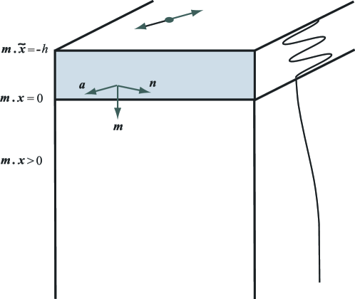
Figure 1: Sketch of the layered formation. The wave propagates in the direction of the unit vector $\boldsymbol{n}$, it is polarized along $\boldsymbol{a}$, and the magnitude of its amplitude varies along the direction of the unit vector $\boldsymbol{m}$, normal to the faces of the layer.

To ensure rigid bonding the displacement must be continuous at the interface. The displacements $\boldsymbol{u}$ in the substrate and $\widetilde{\boldsymbol{u}}$ in the layer are given respectively by

$$\boldsymbol{u}=\boldsymbol{x-X}=(\boldsymbol{I}-\boldsymbol{F}^{-1})\boldsymbol{x},\qquad\widetilde{\boldsymbol{u}}=\widetilde{\boldsymbol{x}}-\boldsymbol{X}=(\boldsymbol{I}-\widetilde{\boldsymbol{F}}^{-1})\widetilde{\boldsymbol{x}}.$$ (4.2)

At any point in the interface $\boldsymbol{m\cdot x}=\boldsymbol{m}\cdot\widetilde{\boldsymbol{x}}=0$, we have $\boldsymbol{x}=\widetilde{\boldsymbol{x}}=\alpha\boldsymbol{n}+\beta\boldsymbol{a}$ for some $\alpha$ and $\beta$. Then the displacement continuity $\boldsymbol{u}=\widetilde{\boldsymbol{u}}$ at the interface is equivalent to $\boldsymbol{F}^{-1}(\alpha\boldsymbol{n}+\beta\boldsymbol{a})=\widetilde{\boldsymbol{F}}^{-1}(\alpha\boldsymbol{n}+\beta\boldsymbol{a})$. Because this must hold for all $\alpha$, $\beta$, we conclude that the requirement of displacement continuity is

$$\boldsymbol{F}^{-1}\boldsymbol{n}=\widetilde{\boldsymbol{F}}^{-1}\boldsymbol{n},\qquad\boldsymbol{F}^{-1}\boldsymbol{a}=\widetilde{\boldsymbol{F}}^{-1}\boldsymbol{a}.$$ (4.3)

It then follows that $\boldsymbol{F}^{-1}\boldsymbol{n}\times\boldsymbol{F}^{-1}\boldsymbol{a}=\widetilde{\boldsymbol{F}}^{-1}\boldsymbol{n}\times\widetilde{\boldsymbol{F}}^{-1}\boldsymbol{a}$. Hence, using the identity [25]: $\boldsymbol{F}^{-1}\boldsymbol{n}\times\boldsymbol{F}^{-1}\boldsymbol{a}=(\det\boldsymbol{F})^{-1}\boldsymbol{F}^{T}(\boldsymbol{n}\times\boldsymbol{a})$, and similarly for $\widetilde{\boldsymbol{F}}$, we obtain

$$(\det\boldsymbol{F})^{-1}\boldsymbol{F}^{T}\boldsymbol{m}=(\det\widetilde{\boldsymbol{F}})^{-1}\widetilde{\boldsymbol{F}}^{T}\boldsymbol{m},$$ (4.4)

from which it follows that

$$J^{-2}\boldsymbol{m}\cdot\boldsymbol{B}\boldsymbol{m}=\widetilde{J}^{-2}\boldsymbol{m}\cdot\widetilde{\boldsymbol{B}}\boldsymbol{m}.$$ (4.5)

We note in passing that the unit vector $\boldsymbol{M}$ normal to the faces of the layer in the undeformed state is given by

$$\boldsymbol{M}=(\boldsymbol{m}\cdot\boldsymbol{B}\boldsymbol{m})^{-1/2}\boldsymbol{F}^{T}\boldsymbol{m}=(\boldsymbol{m}\cdot\widetilde{\boldsymbol{B}}\boldsymbol{m})^{-1/2}\widetilde{\boldsymbol{F}}^{T}\boldsymbol{m},$$ (4.6)

and that the thickness $H$ of the layer in the undeformed state is

$$H=h(\boldsymbol{m}\cdot\widetilde{\boldsymbol{B}}\boldsymbol{m})^{-1/2}.$$ (4.7)

Next, we consider the corresponding constant Cauchy stress tensors $\boldsymbol{T}$ and $\widetilde{\boldsymbol{T}}$, in the substrate and the layer, respectively. The equilibrium of the pre-strained state requires that the upper face of the layer be subjected to the traction (deadload) $\boldsymbol{\tau}=\widetilde{\boldsymbol{T}}\boldsymbol{m}$, and that the traction vector be continuous at the interface, $\boldsymbol{Tm}=\widetilde{\boldsymbol{T}}\boldsymbol{m}$. Using the constitutive equations of the layer and of the substrate, this yields

$$\widetilde{\mu}\widetilde{J}^{-1}\boldsymbol{n}\cdot\widetilde{\boldsymbol{B}}\boldsymbol{m}=\mu J^{-1}\boldsymbol{n\cdot Bm},\qquad\widetilde{\mu}\widetilde{J}^{-1}\boldsymbol{a}\cdot\widetilde{\boldsymbol{B}}\boldsymbol{m}=\mu J^{-1}\boldsymbol{a\cdot Bm},$$

$$\textstyle{\frac{1}{2}}\widetilde{G}^{\prime}(\widetilde{J})+\widetilde{\mu}\widetilde{J}^{-1}\boldsymbol{m}\cdot\widetilde{\boldsymbol{B}}\boldsymbol{m}=\textstyle{\frac{1}{2}}G^{\prime}(J)+\mu J^{-1}\boldsymbol{m\cdot Bm}.$$ (4.8)

Using the requirements of continuity of the displacement and of the traction at the interface, we now show how a given initial strain $\widetilde{\boldsymbol{B}}$ in the layer (resulting from a prescribed stress $\widetilde{\boldsymbol{T}}$) determines the initial strain $\boldsymbol{B}$ in the substrate.

First, we note that (4)₃ may alternatively be written as follows, using (4.5),

$$\textstyle{\frac{1}{2}}G^{\prime}(J)+\mu J\widetilde{J}^{-2}\boldsymbol{m}\cdot\widetilde{\boldsymbol{B}}\boldsymbol{m}=\textstyle{\frac{1}{2}}\widetilde{G}^{\prime}(\widetilde{J})+\widetilde{\mu}\widetilde{J}^{-1}\boldsymbol{m}\cdot\widetilde{\boldsymbol{B}}\boldsymbol{m}.$$ (4.9)

Because $\widetilde{\boldsymbol{B}}$ is given, $\widetilde{J}$ and $\boldsymbol{m}\cdot\widetilde{\boldsymbol{B}}\boldsymbol{m}$ are known and so, this is an equation for a single unknown, $J$. It is shown in the Appendix how the strong ellipticity assumption implies that this equation has at most one positive solution for $J$, and one and only one solution if, in addition, it is assumed that $\lim_{J\rightarrow 0}G^{\prime}(J)=-\infty$. Once $J$ is known, then (4.5) determines $\boldsymbol{m\cdot Bm}$, and (4)_1,2 determine $\boldsymbol{n\cdot Bm}$ and $\boldsymbol{a\cdot Bm}$. Explicitly,

$$\boldsymbol{m\cdot Bm}=(J/\widetilde{J})^{2}\boldsymbol{m}\cdot\widetilde{\boldsymbol{B}}\boldsymbol{m},\qquad\boldsymbol{n\cdot Bm}=(J/\widetilde{J})(\widetilde{\mu}/\mu)\boldsymbol{n}\cdot\widetilde{\boldsymbol{B}}\boldsymbol{m},\\ \boldsymbol{a\cdot Bm}=(J/\widetilde{J})(\widetilde{\mu}/\mu)\boldsymbol{a}\cdot\widetilde{\boldsymbol{B}}\boldsymbol{m}.$$ (4.10)

In order to obtain all the components of $\boldsymbol{B}$ in the orthonormal triad ($\boldsymbol{n},\boldsymbol{a},\boldsymbol{m}$), we still need to determine $\boldsymbol{a\cdot Ba}$, $\boldsymbol{n\cdot Bn}$, $\boldsymbol{n\cdot Ba}$. For this purpose, we note that the displacement continuity requirement (4.3) implies that

$$\boldsymbol{n}\cdot\boldsymbol{B}^{-1}\boldsymbol{n}=\boldsymbol{n}\cdot\widetilde{\boldsymbol{B}}^{-1}\boldsymbol{n},\qquad\boldsymbol{a}\cdot\boldsymbol{B}^{-1}\boldsymbol{a}=\boldsymbol{a}\cdot\widetilde{\boldsymbol{B}}^{-1}\boldsymbol{a},\qquad\boldsymbol{n}\cdot\boldsymbol{B}^{-1}\boldsymbol{a}=\boldsymbol{n}\cdot\widetilde{\boldsymbol{B}}^{-1}\boldsymbol{a}.$$ (4.11)

Using $\boldsymbol{n}=\boldsymbol{a}\times\boldsymbol{m}$ in (4.11)₁, and the identity

$$\boldsymbol{n}\cdot\boldsymbol{B}^{-1}\boldsymbol{n}=J^{-2}[(\boldsymbol{a}\cdot\boldsymbol{B}\boldsymbol{a})(\boldsymbol{m}\cdot\boldsymbol{B}\boldsymbol{m})-(\boldsymbol{a}\cdot\boldsymbol{B}\boldsymbol{m})^{2}],$$ (4.12)

valid also with $\widetilde{\boldsymbol{B}}$ instead of $\boldsymbol{B}$, we obtain

$$\boldsymbol{a}\cdot\boldsymbol{B}\boldsymbol{a}=\boldsymbol{a}\cdot\widetilde{\boldsymbol{B}}\boldsymbol{a}-\frac{(\boldsymbol{a}\cdot\widetilde{\boldsymbol{B}}\boldsymbol{m})^{2}}{\boldsymbol{m}\cdot\widetilde{\boldsymbol{B}}\boldsymbol{m}}+\frac{(\boldsymbol{a}\cdot\boldsymbol{B}\boldsymbol{m})^{2}}{\boldsymbol{m}\cdot\boldsymbol{B}\boldsymbol{m}}.$$ (4.13)

Recalling (4.10)_1,3, we obtain

$$\boldsymbol{a}\cdot\boldsymbol{B}\boldsymbol{a}=\boldsymbol{a}\cdot\widetilde{\boldsymbol{B}}\boldsymbol{a}+\left(\frac{\widetilde{\mu}^{2}}{\mu^{2}}-1\right)\frac{(\boldsymbol{a}\cdot\widetilde{\boldsymbol{B}}\boldsymbol{m})^{2}}{\boldsymbol{m}\cdot\widetilde{\boldsymbol{B}}\boldsymbol{m}}.$$ (4.14)

A similar procedure, using $\boldsymbol{a}=\boldsymbol{m}\times\boldsymbol{n}$ in (4.11)₂, yields

$$\boldsymbol{n}\cdot\boldsymbol{B}\boldsymbol{n}=\boldsymbol{n}\cdot\widetilde{\boldsymbol{B}}\boldsymbol{n}+\left(\frac{\widetilde{\mu}^{2}}{\mu^{2}}-1\right)\frac{(\boldsymbol{n}\cdot\widetilde{\boldsymbol{B}}\boldsymbol{m})^{2}}{\boldsymbol{m}\cdot\widetilde{\boldsymbol{B}}\boldsymbol{m}}.$$ (4.15)

Finally, (4.11)₃ with $\boldsymbol{n}=\boldsymbol{a}\times\boldsymbol{m}$ and $\boldsymbol{a}=\boldsymbol{m}\times\boldsymbol{n}$ yields

$$\boldsymbol{n}\cdot\boldsymbol{B}\boldsymbol{a}=\boldsymbol{n}\cdot\widetilde{\boldsymbol{B}}\boldsymbol{a}+\left(\frac{\widetilde{\mu}^{2}}{\mu^{2}}-1\right)\frac{(\boldsymbol{n}\cdot\widetilde{\boldsymbol{B}}\boldsymbol{m})(\boldsymbol{a}\cdot\widetilde{\boldsymbol{B}}\boldsymbol{m})}{\boldsymbol{m}\cdot\widetilde{\boldsymbol{B}}\boldsymbol{m}}.$$ (4.16)

To summarize: when the (constant) left Cauchy-Green strain tensor $\widetilde{\boldsymbol{B}}$ in the layer is prescribed, then the (constant) left Cauchy-Green strain tensor $\boldsymbol{B}$ in the substrate is uniquely determined. First, $J$ is uniquely determined from equation (4.9). Then, all the components of $\boldsymbol{B}$ in the orthonormal triad ($\boldsymbol{n},\boldsymbol{m},\boldsymbol{a}$) are explicitly given by equations (4.10)_1,2,3, (4.14), (4.15), (4.16).

In order to use the exact wave solutions described in Section 3, we shall assume from now on that the condition (3.11) is fulfilled in the layer, which, by (4.10)₂ implies that it is also fulfilled in the substrate :

$$\boldsymbol{n}\cdot\boldsymbol{B}\boldsymbol{m}=0,\qquad\boldsymbol{n}\cdot\widetilde{\boldsymbol{B}}\boldsymbol{m}=0.$$ (4.17)

Then, the equations for the other components of $\boldsymbol{B}$ reduce to

$$\boldsymbol{m\cdot Bm}=(J/\widetilde{J})^{2}\boldsymbol{m}\cdot\widetilde{\boldsymbol{B}}\boldsymbol{m}, \boldsymbol{a\cdot Bm}=(J/\widetilde{J})(\widetilde{\mu}/\mu)\boldsymbol{a}\cdot\widetilde{\boldsymbol{B}}\boldsymbol{m},$$

$$\boldsymbol{a}\cdot\boldsymbol{B}\boldsymbol{a}=\boldsymbol{a}\cdot\widetilde{\boldsymbol{B}}\boldsymbol{a}+\left(\frac{\widetilde{\mu}^{2}}{\mu^{2}}-1\right)\frac{(\boldsymbol{a}\cdot\widetilde{\boldsymbol{B}}\boldsymbol{m})^{2}}{\boldsymbol{m}\cdot\widetilde{\boldsymbol{B}}\boldsymbol{m}}, \boldsymbol{n}\cdot\boldsymbol{B}\boldsymbol{n}=\boldsymbol{n}\cdot\widetilde{\boldsymbol{B}}\boldsymbol{n},$$

$$\boldsymbol{n}\cdot\boldsymbol{B}\boldsymbol{a}=\boldsymbol{n}\cdot\widetilde{\boldsymbol{B}}\boldsymbol{a}.$$ (4.18)

In tensorial form, the expression of $\boldsymbol{B}$ in terms of $\widetilde{\boldsymbol{B}}$ is given by

$$(\boldsymbol{m}\cdot\widetilde{\boldsymbol{B}}\boldsymbol{m})\boldsymbol{B}=(\boldsymbol{m}\cdot\widetilde{\boldsymbol{B}}\boldsymbol{m})\widetilde{\boldsymbol{B}}-\widetilde{\boldsymbol{B}}\boldsymbol{m}\otimes\widetilde{\boldsymbol{B}}\boldsymbol{m}\\ +\left[(\widetilde{\mu}/\mu)(\boldsymbol{a}\cdot\widetilde{\boldsymbol{B}}\boldsymbol{m})\boldsymbol{a}+(J/\widetilde{J})(\boldsymbol{m}\cdot\widetilde{\boldsymbol{B}}\boldsymbol{m})\boldsymbol{m}\right]\\ \otimes\left[(\widetilde{\mu}/\mu)(\boldsymbol{a}\cdot\widetilde{\boldsymbol{B}}\boldsymbol{m})\boldsymbol{a}+(J/\widetilde{J})(\boldsymbol{m}\cdot\widetilde{\boldsymbol{B}}\boldsymbol{m})\boldsymbol{m}\right].$$ (4.19)

In particular, we note that $\boldsymbol{Bn}=\widetilde{\boldsymbol{B}}\boldsymbol{n}$.

5 Large amplitude Love wave

Now we look at wave propagation in the initially deformed structure. In the substrate, we require that amplitude of the wave decays in the direction of $\boldsymbol{m}$, and hence the displacement field $\boldsymbol{u}$ is assumed to be of the form (3.15). In the layer, we consider an unattenuated time-harmonic displacement field $\widetilde{\boldsymbol{u}}$ of the form (3.14). As in the classical case, we wish to combine these exact wave solutions in order to obtain a global time-harmonic wave motion with propagation speed $v$. Note that both displacement fields need to be of the same angular frequency, and hence the same wavenumber, in order to satisfy boundary conditions at the interface. Thus, using (3.15) for the substrate and (3.14) for the layer, we write

$$\boldsymbol{u}(\boldsymbol{x},t)=A\exp\left(-\frac{\gamma}{v_{\boldsymbol{m}}}\boldsymbol{m}\cdot\boldsymbol{x}\right)\cos k(\boldsymbol{n}\cdot\boldsymbol{x}-vt)\boldsymbol{a},$$ (5.1)

and

$$\widetilde{\boldsymbol{u}}(\boldsymbol{x},t)=\left[B\sin(\frac{\kappa}{\widetilde{v}_{\boldsymbol{m}}}\boldsymbol{m}\cdot\boldsymbol{x})+C\cos(\frac{\kappa}{\widetilde{v}_{\boldsymbol{m}}}\boldsymbol{m}\cdot\boldsymbol{x})\right]\cos k(\boldsymbol{n}\cdot\boldsymbol{x}-vt)\boldsymbol{a},$$ (5.2)

where

$$k=\frac{\kappa}{\sqrt{v^{2}-\widetilde{v}^{2}_{\boldsymbol{n}}}}=\frac{\gamma}{\sqrt{v^{2}_{\boldsymbol{n}}-v^{2}}},$$ (5.3)

is the wavenumber. Here, in accordance with (3.13), the body waves speeds $v_{\boldsymbol{n}}$, $v_{\boldsymbol{m}}$, $\widetilde{v}_{\boldsymbol{n}}$, $\widetilde{v}_{\boldsymbol{m}}$ are given by

$$\rho_{0}v^{2}_{\boldsymbol{m}}=\mu\,\boldsymbol{m\cdot Bm},\qquad\rho_{0}v^{2}_{\boldsymbol{n}}=\mu\,\boldsymbol{n\cdot Bn},\\ \widetilde{\rho}_{0}\widetilde{v}^{2}_{\boldsymbol{m}}=\widetilde{\mu}\,\boldsymbol{m}\cdot\widetilde{\boldsymbol{B}}\boldsymbol{m},\qquad\widetilde{\rho}_{0}\widetilde{v}^{2}_{\boldsymbol{n}}=\widetilde{\mu}\,\boldsymbol{n}\cdot\widetilde{\boldsymbol{B}}\boldsymbol{n},$$ (5.4)

and the Love wave speed $v$ has to satisfy

$$\widetilde{v}^{2}_{\boldsymbol{n}}<v^{2}<v^{2}_{\boldsymbol{n}}.$$ (5.5)

Notice that this is possible only when $v^{2}_{\boldsymbol{n}}>\widetilde{v}^{2}_{\boldsymbol{n}}$, or equivalently, recalling $\boldsymbol{n\cdot Bn}=\boldsymbol{n}\cdot\widetilde{\boldsymbol{B}}\boldsymbol{n}$, when $\mu/\rho_{0}>\widetilde{\mu}/\widetilde{\rho}_{0}$. Thus, Love waves require the combination of a ‘slow’ (or ‘soft’) layer over a ‘fast’ (or ‘hard’) substrate, independently of the initial pre-strain.

We now show that the boundary conditions may be satisfied. This leads to the dispersion equation (a relation between $k$ and $v$) and the determination of the constants $A$, $B$, $C$ in terms of a single parameter characterizing the amplitude of the wave.

The first boundary condition to enforce is that the displacement is continuous at the layer/substrate interface $\boldsymbol{m\cdot x}=0$. Using (5.1) and (5.2), this gives

$$A=C.$$ (5.6)

The second boundary condition is the continuity of the traction vector at the layer/substrate interface $\boldsymbol{m}\cdot\boldsymbol{x}=0$. Using (3.16), and applying it to the wave motion (5.1), we obtain, for the traction $\boldsymbol{t}$ on a plane $\boldsymbol{m}\cdot\boldsymbol{x}=\mbox{\it constant}\,$ in the substrate,

$$\boldsymbol{t}=\boldsymbol{Tm}-\gamma\rho v_{\boldsymbol{m}}A\exp\left(-\frac{\gamma}{v_{\boldsymbol{m}}}\boldsymbol{m}\cdot\boldsymbol{x}\right)\cos k(\boldsymbol{n}\cdot\boldsymbol{x}-vt)\boldsymbol{a},$$ (5.7)

where $\rho=J^{-1}\rho_{0}$ is the mass density of the substrate in the intermediate configuration. Similarly for the traction $\widetilde{\boldsymbol{t}}$ on a plane $\boldsymbol{m}\cdot\boldsymbol{x}=\mbox{\it constant}\,$ in the layer, we find

$$\widetilde{\boldsymbol{t}}=\widetilde{\boldsymbol{T}}\boldsymbol{m}+\kappa\widetilde{\rho}\,\widetilde{v}_{\boldsymbol{m}}\left[B\cos\left(\frac{\kappa}{\widetilde{v}_{\boldsymbol{m}}}\boldsymbol{m}\cdot\boldsymbol{x}\right)-C\sin\left(\frac{\kappa}{\widetilde{v}_{\boldsymbol{m}}}\boldsymbol{m}\cdot\boldsymbol{x}\right)\right]\cos k\left(\boldsymbol{n}\cdot\boldsymbol{x}-vt\right)\boldsymbol{a}.$$ (5.8)

where $\widetilde{\rho}=J^{-1}\widetilde{\rho}_{0}$ is the mass density of the layer in the intermediate configuration. Also, recall that $\boldsymbol{Tm}=\widetilde{\boldsymbol{T}}\boldsymbol{m}=\boldsymbol{\tau}$, where $\boldsymbol{\tau}$ is the constant traction (deadload) applied at the upper face of the layer. Hence the condition $\boldsymbol{t}=\widetilde{\boldsymbol{t}}$ at the layer/substrate interface $\boldsymbol{m}\cdot\boldsymbol{x}=0$ reads

$$\gamma\rho v_{\boldsymbol{m}}A+\kappa\widetilde{\rho}\,\widetilde{v}_{\boldsymbol{m}}B=0.$$ (5.9)

The third boundary condition is that, at the upper face of the layer $\boldsymbol{m}\cdot\boldsymbol{x}=-h$, the wave creates no traction in addition to the static traction (deadload) $\boldsymbol{\tau}$. Using (5.8), this yields

$$B\cos(\frac{\kappa}{\widetilde{v}_{\boldsymbol{m}}}h)+C\sin(\frac{\kappa}{\widetilde{v}_{\boldsymbol{m}}}h)=0.$$ (5.10)

Equations (5.6), (5.9), (5.10) form an algebraic linear homogeneous system for the three unknowns $A$, $B$, $C$. Writing the condition for non-trivial solutions and using (5.3), we arrive at the following dispersion equation relating the wave speed $v$ to the wave number $k$,

$$\tan\left[kh\sqrt{\frac{v^{2}-\widetilde{v}^{2}_{\boldsymbol{n}}}{\widetilde{v}^{2}_{\boldsymbol{m}}}}\right]-\frac{\rho v_{\boldsymbol{m}}}{\widetilde{\rho}\,\widetilde{v}_{\boldsymbol{m}}}\sqrt{\frac{v^{2}_{\boldsymbol{n}}-v^{2}}{v^{2}-\widetilde{v}^{2}_{\boldsymbol{n}}}}=0.$$ (5.11)

Let $c$ and $\widetilde{c}$ denote the transverse bulk wave speeds in the underformed substrate and layer, respectively: $c^{2}=\mu/\rho_{0}$, $\widetilde{c}^{2}=\widetilde{\mu}/\widetilde{\rho}_{0}$. Using (4) and (5.4), we note that $v^{2}_{\boldsymbol{n}}/\widetilde{v}^{2}_{\boldsymbol{n}}=c^{2}/\widetilde{c}^{2}$ and $\rho v_{\boldsymbol{m}}/(\widetilde{\rho}\widetilde{v}_{\boldsymbol{m}})=\rho_{0}c/(\widetilde{\rho}_{0}\widetilde{c})$, so that the dispersion equation (5.11) may also be written as

$$\tan\left[kh(\widetilde{v}_{\boldsymbol{n}}/\widetilde{v}_{\boldsymbol{m}})\sqrt{(v/\widetilde{v}_{\boldsymbol{n}})^{2}-1}\right]-\frac{\rho_{0}c}{\widetilde{\rho}_{0}\widetilde{c}}\sqrt{\frac{(c/\widetilde{c})^{2}-(v/\widetilde{v}_{\boldsymbol{n}})^{2}}{(v/\widetilde{v}_{\boldsymbol{n}})^{2}-1}}=0.$$ (5.12)

In the absence of pre-strain, $\boldsymbol{B}=\widetilde{\boldsymbol{B}}=\boldsymbol{I}$, $J=\widetilde{J}=1$, hence $v^{2}_{\boldsymbol{n}}=v^{2}_{\boldsymbol{m}}=c^{2}$ in the substrate and $\widetilde{v}^{2}_{\boldsymbol{n}}=\widetilde{v}^{2}_{\boldsymbol{m}}=\widetilde{c}^{2}$ in the layer, so that this dispersion equation specializes to

$$\tan\left[kh\sqrt{(v/\widetilde{c})^{2}-1}\right]-\frac{\rho_{0}c}{\widetilde{\rho}_{0}\widetilde{c}}\sqrt{\frac{(c/\widetilde{c})^{2}-(v/\widetilde{c})^{2}}{(v/\widetilde{c})^{2}-1}}=0,$$ (5.13)

which coincides with the dispersion equation of linear isotropic elasticity [29]. From a practical point of view, any dispersion curve obtained from (5.13) as a plot of $v/\widetilde{c}$ against $kh$ for a given choice of $\rho_{0}/\widetilde{\rho}_{0}$ and $c/\widetilde{c}$ can be used in the present context of (5.12), by identifying $v/\widetilde{c}$ with $v/\widetilde{v}_{\boldsymbol{n}}$ and $kh$ with $(\widetilde{v}_{\boldsymbol{n}}/\widetilde{v}_{\boldsymbol{m}})kh$, see Willson [11] for similar results in the small-on-large theory. A typical plot for the different wave modes is presented in Fig.2. Of course, the scope of the results is now richer because they include large amplitudes and pre-stress.

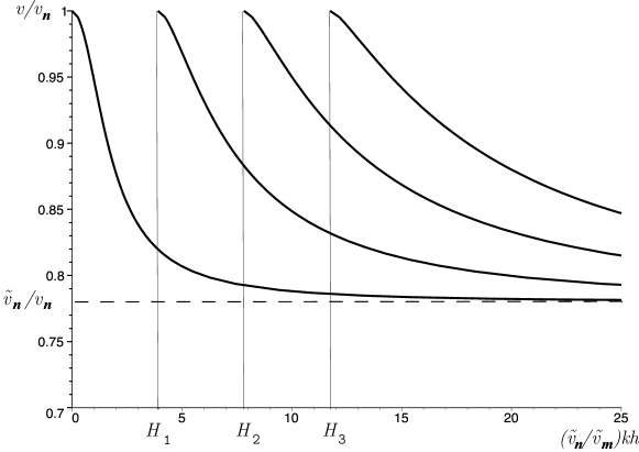
Figure 2: Dispersion curves for successive Love wave modes in a pre-strained configuration. Here $H_{l}=l\pi/\sqrt{(c/\widetilde{c})^{2}-1}$, ($l=1,2,3,4,\ldots$). Thus, for $0<kh<(\widetilde{v}_{\boldsymbol{m}}/\widetilde{v}_{\boldsymbol{n}})H_{1}$, only one mode may propagate (fundamental mode). For $(\widetilde{v}_{\boldsymbol{m}}/\widetilde{v}_{\boldsymbol{n}})H_{l}<kh<(\widetilde{v}_{\boldsymbol{m}}/\widetilde{v}_{\boldsymbol{n}})H_{l+1}$, $l+1$ modes may propagate.

When the dispersion equation (5.11) is satisfied, the solution of the linear homogeneous system (5.6), (5.9), (5.10) for $A$, $B$, $C$ is

$$A=\alpha\cos\left(\frac{\kappa}{\widetilde{v}_{\boldsymbol{m}}}h\right),\qquad B=-\alpha\sin\left(\frac{\kappa}{\widetilde{v}_{\boldsymbol{m}}}h\right),\qquad C=\alpha\cos\left(\frac{\kappa}{\widetilde{v}_{\boldsymbol{m}}}h\right),$$ (5.14)

where $\alpha$ is arbitrary. Thus $A$, $B$, $C$ are expressed in terms of a single parameter $\alpha$ characterizing the amplitude of the Love wave.

Finally, we now denote by $(\eta,\xi,\zeta)$ the Cartesian coordinates along ($\boldsymbol{n},\boldsymbol{a},\boldsymbol{m}$),

$$\eta=\boldsymbol{n}\cdot\boldsymbol{x},\qquad\xi=\boldsymbol{a}\cdot\boldsymbol{x},\qquad\zeta=\boldsymbol{m}\cdot\boldsymbol{x},$$ (5.15)

and we find that the displacement fields (5.1) (5.2) are

$$\boldsymbol{u}=\alpha\cos\left(\frac{\kappa}{\widetilde{v}_{\boldsymbol{m}}}h\right)\exp\left(-\frac{\gamma}{v_{\boldsymbol{m}}}\zeta\right)\cos k(\eta-vt)\boldsymbol{a},$$

$$\widetilde{\boldsymbol{u}}=\alpha\cos\frac{\kappa}{\widetilde{v}_{\boldsymbol{m}}}(h+\zeta)\cos k(\eta-vt)\boldsymbol{a},$$ (5.16)

or equivalently, recalling (5.3),

$$\boldsymbol{u} = \alpha\cos\left[kh\sqrt{\frac{v^{2}-\widetilde{v}^{2}_{\boldsymbol{n}}}{\widetilde{v}^{2}_{\boldsymbol{m}}}}\right]\exp\left[-k\zeta\sqrt{\frac{v^{2}_{\boldsymbol{n}}-v^{2}}{v^{2}_{\boldsymbol{m}}}}\right]\cos k(\eta-vt)\boldsymbol{a},$$ (5.17)

$$\widetilde{\boldsymbol{u}} = \alpha\cos\left[k(h+\zeta)\sqrt{\frac{v^{2}-\widetilde{v}^{2}_{\boldsymbol{n}}}{\widetilde{v}^{2}_{\boldsymbol{m}}}}\right]\cos k(\eta-vt)\boldsymbol{a}.$$ (5.18)

6 Energy density and energy flux

Here we compute the energy flux and the energy density associated with a motion of the type (3.2) in compressible neo-Hookean materials. Let $W$ and $\overline{W}$ be the strain energy densities corresponding, respectively, to the static deformation (3.1) and to the motion (3.2), both measured per unit volume of the undeformed state. Then, the energy density ${\cal E}$, measured per unit volume of the homogeneously deformed state (3.1), and the corresponding energy flux vector $\boldsymbol{{\cal R}}$ are [27]

$${\cal E}=\textstyle{\frac{1}{2}}\rho\dot{\overline{\boldsymbol{x}}}\cdot\dot{\overline{\boldsymbol{x}}}+J^{-1}(\overline{W}-W),\qquad{\cal R}_{k}=-\dot{\overline{x}}_{i}\overline{P}_{ik},$$ (6.1)

where the Piola-Kirchhoff stress tensor $\overline{\boldsymbol{P}}$ with respect to the state of homogeneous static deformation is defined by (3.4). They satisfy the energy balance equation

$$(\partial{\cal E}/\partial t)+(\partial{\cal R}_{k}/\partial x_{k})=0,$$ (6.2)

where $x_{k}$ are the coordinates in the state of homogeneous static deformation, and the partial derivative with respect to time is taken at fixed $\boldsymbol{x}$.

We now evaluate the energy density and the energy flux vector for the wave motion (5.16)₂ in the layer, and for the wave motion (5.16)₁ in the substrate. Using (5.16)₂, we obtain for the layer

$$\widetilde{{\cal E}} = \textstyle{\frac{1}{2}}\widetilde{\rho}k^{2}\alpha^{2}(v^{2}+\widetilde{v}^{2}_{\boldsymbol{n}})\cos^{2}\frac{\kappa}{\widetilde{v}_{\boldsymbol{m}}}(h+\zeta)\sin^{2}k(\eta-vt)$$

$$+\textstyle{\frac{1}{2}}\widetilde{\rho}k^{2}\alpha^{2}(v^{2}-\widetilde{v}^{2}_{\boldsymbol{n}})\sin^{2}\frac{\kappa}{\widetilde{v}_{\boldsymbol{m}}}(h+\zeta)\cos^{2}k(\eta-vt)$$

$$-\alpha\ \boldsymbol{a}\!\cdot\![\frac{\kappa}{\widetilde{v}_{\boldsymbol{m}}}\sin\frac{\kappa}{\widetilde{v}_{\boldsymbol{m}}}(h+\zeta)\cos k(\eta-vt)\widetilde{\boldsymbol{T}}\boldsymbol{m}$$

$$+k\cos\frac{\kappa}{\widetilde{v}_{\boldsymbol{m}}}(h+\zeta)\sin k(\eta-vt)\widetilde{\boldsymbol{T}}\boldsymbol{n}],$$

$$\widetilde{\boldsymbol{{\cal R}}} = \cos\frac{\kappa}{\widetilde{v}_{\boldsymbol{m}}}(h+\zeta)\sin k(\eta-vt)\{-vk\alpha\widetilde{\boldsymbol{T}}\boldsymbol{a}$$

$$+\alpha^{2}kv\widetilde{\mu}\widetilde{J}^{-1}[\frac{\kappa}{\widetilde{v}_{\boldsymbol{m}}}\sin\frac{\kappa}{\widetilde{v}_{\boldsymbol{m}}}(h+\zeta)\cos k(\eta-vt)\widetilde{\boldsymbol{B}}\boldsymbol{m}$$

$$+k\cos\frac{\kappa}{\widetilde{v}_{\boldsymbol{m}}}(h+\zeta)\sin k(\eta-vt)\widetilde{\boldsymbol{B}}\boldsymbol{n}]\}.$$

Using (5.16)₁, we obtain for the substrate

$${\cal E} = \textstyle{\frac{1}{2}}\rho k^{2}\alpha^{2}\cos^{2}(\frac{\kappa}{\widetilde{v}_{\boldsymbol{m}}}h)\mbox{exp}(\frac{-2\gamma}{v_{\boldsymbol{m}}}\zeta)[v^{2}_{\boldsymbol{n}}+v^{2}\sin^{2}k(\eta-vt)-v^{2}\cos^{2}k(\eta-vt)]$$ (6.5)

$$-\alpha\cos(\frac{\kappa}{\widetilde{v}_{\boldsymbol{m}}}h)\mbox{exp}(\frac{-\gamma}{v_{\boldsymbol{m}}}\zeta)\ \boldsymbol{a}\!\cdot\![\frac{\gamma}{v_{\boldsymbol{m}}}\cos k(\eta-vt)\boldsymbol{T}\boldsymbol{m}$$

$$+k\sin k(\eta-vt)\boldsymbol{T}\boldsymbol{n}],\;$$

$$\boldsymbol{{\cal R}} = -vk\alpha\cos(\frac{\kappa}{\widetilde{v}_{\boldsymbol{m}}}h)\sin k(\eta-vt)\mbox{exp}(\frac{-\gamma}{v_{\boldsymbol{m}}}\zeta)\boldsymbol{T}\boldsymbol{a}$$

$$+\alpha^{2}kv\mu J^{-1}\cos^{2}(\frac{\kappa}{\widetilde{v}_{\boldsymbol{m}}}h)\mbox{exp}(\frac{-2\gamma}{v_{\boldsymbol{m}}}\zeta)[\frac{\gamma}{v_{\boldsymbol{m}}}\cos k(\eta-vt)\boldsymbol{B}\boldsymbol{m}$$

$$+k\sin k(\eta-vt)\boldsymbol{B}\boldsymbol{n}].$$

Mean energy densities and mean energy fluxes are obtained by averaging over a period in time at fixed $\boldsymbol{x}$,

$$\langle{\cal E}\rangle=(\omega/2\pi)\int_{0}^{2\pi/\omega}{\cal E}(\boldsymbol{x},t)\,dt,\qquad\langle{\boldsymbol{{\cal R}}}\rangle=(\omega/2\pi)\int_{0}^{2\pi/\omega}\boldsymbol{{\cal R}}(\boldsymbol{x},t)\,dt.$$ (6.7)

Using (6), (6), (6.7), we find the mean energy density and the mean energy flux in the layer as

$$\langle\widetilde{{\cal E}}\rangle=\textstyle{\frac{1}{4}}\widetilde{\rho}k^{2}\alpha^{2}\{v^{2}+\widetilde{v}^{2}_{\boldsymbol{n}}[\cos^{2}\frac{\kappa}{\widetilde{v}_{\boldsymbol{m}}}(h+\zeta)-\sin^{2}\frac{\kappa}{\widetilde{v}_{\boldsymbol{m}}}(h+\zeta)]\},$$

$$\langle\widetilde{{\boldsymbol{{\cal R}}}}\rangle=\textstyle{\frac{1}{2}}vk^{2}\alpha^{2}\widetilde{\mu}\widetilde{J}^{-1}\cos^{2}\frac{\kappa}{\widetilde{v}_{\boldsymbol{m}}}(h+\zeta)\ \widetilde{\boldsymbol{B}}\boldsymbol{n}.$$ (6.8)

Using (6.5), (6), (6.7), we find the mean energy density and the mean energy flux in the substrate as

$$\langle{\cal E}\rangle=\textstyle{\frac{1}{2}}\rho v^{2}_{\boldsymbol{n}}k^{2}\alpha^{2}\cos^{2}(\frac{\kappa}{\widetilde{v}_{\boldsymbol{m}}}h)\mbox{exp}(\frac{-2\gamma}{v_{\boldsymbol{m}}}\zeta),$$

$$\langle{\boldsymbol{{\cal R}}}\rangle=\textstyle{\frac{1}{2}}vk^{2}\alpha^{2}\mu J^{-1}\cos^{2}(\frac{\kappa}{\widetilde{v}_{\boldsymbol{m}}}h)\ \mbox{exp}(\frac{-2\gamma}{v_{\boldsymbol{m}}}\zeta)\ \boldsymbol{B}\boldsymbol{n}.$$ (6.9)

The mean energy flux in the layer and the mean energy flux in the substrate are both along $\widetilde{\boldsymbol{B}}\boldsymbol{n}=\boldsymbol{Bn}$, thus along the same direction, parallel to the interface. In general, this direction is not along the propagation direction $\boldsymbol{n}$. This is an effect of the anisotropy induced by the pre-strain. However, in the special case when $\boldsymbol{n}$ is along a principal direction of $\boldsymbol{B}$ and $\widetilde{\boldsymbol{B}}$, the mean energy fluxes are along $\boldsymbol{n}$.

Also, we note that at the interface $\zeta=0$, the mean energy flux $\langle{\boldsymbol{{\cal R}}}\rangle_{0}$ (say) in the substrate is related to the mean energy flux $\langle\widetilde{{\boldsymbol{{\cal R}}}}\rangle_{0}$ (say) in the layer through

$$\widetilde{\mu}^{-1}\widetilde{J}\langle\widetilde{{\boldsymbol{{\cal R}}}}\rangle_{0}=\mu^{-1}J\langle{\boldsymbol{{\cal R}}}\rangle_{0}.$$ (6.10)

Similarly, for the mean energy densities $\langle{\cal E}\rangle_{0}$ and $\langle\widetilde{{\cal E}}\rangle_{0}$ at the interface $\zeta=0$ , we find

$$\widetilde{\mu}^{-1}\widetilde{J}\frac{\langle\widetilde{{\cal E}}\rangle_{0}}{(v/\widetilde{v}_{\boldsymbol{n}})^{2}+\cos(2\frac{\kappa}{\widetilde{v}_{\boldsymbol{m}}}h)}=\mu^{-1}J\frac{\langle{\cal E}\rangle_{0}}{1+\cos(2\frac{\kappa}{\widetilde{v}_{\boldsymbol{m}}}h)}.$$ (6.11)

Recalling that $v^{2}>\widetilde{v}^{2}_{\boldsymbol{n}}$, we note in particular that $\widetilde{\mu}^{-1}\widetilde{J}\langle\widetilde{{\cal E}}\rangle_{0}>\mu^{-1}J\langle{\cal E}\rangle_{0}$.

We now consider the energy flux velocity defined as the mean energy flux vector divided by the mean energy density. For the energy flux velocity $\widetilde{\boldsymbol{g}}$ wave in the layer, we have

$$\widetilde{\boldsymbol{g}}=\frac{\langle\widetilde{{\boldsymbol{{\cal R}}}}\rangle}{\langle\widetilde{{\cal E}}\rangle}=v\,\frac{1+\cos 2\frac{\kappa}{\widetilde{v}_{\boldsymbol{m}}}(h+\zeta)}{(v/\widetilde{v}_{\boldsymbol{n}})^{2}+\cos 2\frac{\kappa}{\widetilde{v}_{\boldsymbol{m}}}(h+\zeta)}\,\frac{\widetilde{\boldsymbol{B}}\boldsymbol{n}}{(\boldsymbol{n}\cdot\widetilde{\boldsymbol{B}}\boldsymbol{n})},$$ (6.12)

and for the energy flux velocity $\boldsymbol{g}$ in the substrate, we have

$$\boldsymbol{g}=\frac{\langle{\boldsymbol{{\cal R}}}\rangle}{\langle{\cal E}\rangle}=v\,\frac{\boldsymbol{B}\boldsymbol{n}}{(\boldsymbol{n}\cdot\boldsymbol{B}\boldsymbol{n})}.$$ (6.13)

In the layer, the energy flux velocity depends on the depth $\zeta$ whilst in the substrate, the energy flux velocity is the same at all points. This is because the wave motion in the substrate consists of a single train of inhomogeneous plane waves. On the contrary, the wave motion in the layer may be viewed as a superposition of trains of homogeneous plane waves. Because $\widetilde{\boldsymbol{B}}\boldsymbol{n}=\boldsymbol{Bn}$, the energy flux velocities are related through

$$[(v/\widetilde{v}_{\boldsymbol{n}})^{2}+\cos 2\frac{\kappa}{\widetilde{v}_{\boldsymbol{m}}}(h+\zeta)]\widetilde{\boldsymbol{g}}=[1+\cos 2\frac{\kappa}{\widetilde{v}_{\boldsymbol{m}}}(h+\zeta)]\boldsymbol{g}.$$ (6.14)

Also, because $v^{2}>\widetilde{v}^{2}_{\boldsymbol{n}}$, we note that the energy flux velocity at any point of the layer is smaller in magnitude that the energy flux velocity in the substrate. Finally we note that

$$\boldsymbol{g}\cdot\boldsymbol{n}=v,\qquad\boldsymbol{g}\cdot\boldsymbol{m}=0,$$ (6.15)

in accordance with previous results about finite amplitude inhomogeneous plane waves in unbounded deformed Blatz-Ko materials [17] [18]. These relations are the same as those derived by Hayes in the context of linear theories [26].

We now define total mean energy densities and total mean energy fluxes as

$$\langle\widetilde{{\cal E}}\rangle_{T}=\int^{0}_{-h}\langle\widetilde{{\cal E}}(\zeta)\rangle\text{d}\zeta,\ \langle\widetilde{{\boldsymbol{{\cal R}}}}\rangle_{T}=\int^{0}_{-h}\langle\widetilde{{\boldsymbol{{\cal R}}}}(\zeta)\rangle\text{d}\zeta,$$

$$\langle{\cal E}\rangle_{T}=\int^{\infty}_{0}\langle{\cal E}(\zeta)\rangle\text{d}\zeta,\ \langle{\boldsymbol{{\cal R}}}\rangle_{T}=\int^{\infty}_{0}\langle{\boldsymbol{{\cal R}}}(\zeta)\rangle\text{d}\zeta.$$ (6.16)

The total mean energy density $\langle\widetilde{{\cal E}}\rangle_{T}$ is the wave energy in the layer $(-h<\zeta=\boldsymbol{m}\cdot\boldsymbol{x}<0)$ per unit length (along $\boldsymbol{n}$) and per unit width (along $\boldsymbol{a}$) of the layer. Similarly, the total mean energy density $\langle{\cal E}\rangle_{T}$ is the energy in the substrate $(0<\zeta=\boldsymbol{m}\cdot\boldsymbol{x}<\infty)$ per unit length (along $\boldsymbol{n}$) and per unit width (along $\boldsymbol{a}$) of the substrate. The total mean energy flux $\langle\widetilde{{\boldsymbol{{\cal R}}}}\rangle_{T}$ is the energy flux characterizing the rate at which energy flows through a normal section of the layer $(-h<\zeta=\boldsymbol{m}\cdot\boldsymbol{x}<0)$ per unit width of this section. Similarly, the total mean energy flux $\langle{\boldsymbol{{\cal R}}}\rangle_{T}$ is the energy flux characterizing the rate at which energy flows through a normal section of the substrate $(-h<\zeta=\boldsymbol{m}\cdot\boldsymbol{x}<0)$ per unit width of this section.

For the wave motion in the layer, we obtain

$$\langle\widetilde{{\cal E}}\rangle_{T}=\textstyle{\frac{1}{4}}\widetilde{\rho}k^{2}\alpha^{2}\left[\widetilde{v}^{2}_{\boldsymbol{n}}\frac{\widetilde{v}_{\boldsymbol{m}}}{2\kappa}\sin(2\frac{\kappa}{\widetilde{v}_{\boldsymbol{m}}}h)+v^{2}h\right],$$

$$\langle\widetilde{{\boldsymbol{{\cal R}}}}\rangle_{T}=\textstyle{\frac{1}{4}}vk^{2}\alpha^{2}\left[\frac{\widetilde{v}_{\textbf{m}}}{2\kappa}\sin(2\frac{\kappa}{\widetilde{v}_{\textbf{m}}}h)+h\right]\widetilde{\mu}\widetilde{J}^{-1}\widetilde{\textbf{B}}\textbf{n},$$ (6.17)

and for the wave motion in the substrate, we obtain

$$\langle{\cal E}\rangle_{T}=\textstyle{\frac{1}{4}}\rho k^{2}\alpha^{2}v^{2}_{\boldsymbol{n}}\frac{v_{\boldsymbol{m}}}{\gamma}\cos^{2}(\frac{\kappa}{\widetilde{v}_{\boldsymbol{m}}}h),\qquad\langle{\boldsymbol{{\cal R}}}\rangle_{T}=\textstyle{\frac{1}{4}}k^{2}\alpha^{2}v\frac{v_{\boldsymbol{m}}}{\gamma}\cos^{2}(\frac{\kappa}{\widetilde{v}_{\textbf{m}}}h)\mu J^{-1}\boldsymbol{B}\boldsymbol{n}.$$ (6.18)

Here we note that the repartition of energy between the layer and the substrate depends on the depth $h$ of the layer, or more precisely, on the dimensionless parameter $kh$ characterizing the ratio of the layer depth to the wavelength.

7 Interface in a principal plane

For a given static strain $\widetilde{\boldsymbol{B}}$ in the layer and a given unit vector $\boldsymbol{m}$, there is, in general, only one direction $\boldsymbol{n}$ in the interface $\boldsymbol{m}\cdot\boldsymbol{x}=\boldsymbol{m}\cdot\widetilde{\boldsymbol{x}}=0$ along which a finite amplitude Love wave as described in Section 5 may propagate. Indeed, because $\boldsymbol{n}\cdot\boldsymbol{m}=\boldsymbol{n}\cdot\widetilde{\boldsymbol{B}}\boldsymbol{m}=0$ is required, $\boldsymbol{n}$ must be along $\boldsymbol{m}\times\widetilde{\boldsymbol{B}}\boldsymbol{m}$. However, if $\boldsymbol{m}$ is along a principal axis of $\widetilde{\boldsymbol{B}}$, then $\boldsymbol{n}\cdot\boldsymbol{m}=\boldsymbol{n}\cdot\widetilde{\boldsymbol{B}}\boldsymbol{m}=0$ is satisfied automatically for any propagation direction $\boldsymbol{n}$ orthogonal to $\boldsymbol{m}$ that is, $\boldsymbol{n}$ can be along any direction in the interface. Here, we consider this special case and give a numerical example showing the effects of strain-induced anisotropy on the wave characteristics.

Calling $\boldsymbol{i},\boldsymbol{j},\boldsymbol{k}$ the unit vectors along the principal axes of $\widetilde{\boldsymbol{B}}$, we write

$$\boldsymbol{n}=\cos\theta\boldsymbol{i}+\sin\theta\boldsymbol{j},\qquad\boldsymbol{a}=-\sin\theta\boldsymbol{i}+\cos\theta\boldsymbol{j},\qquad\boldsymbol{m}=\boldsymbol{k},$$ (7.1)

where the angle $\theta\in[0,2\pi]$ is arbitrary. The left Cauchy-Green strain tensor in the layer is

$$\widetilde{\boldsymbol{B}}=\widetilde{\lambda}_{1}^{2}\boldsymbol{i}\otimes\boldsymbol{i}+\widetilde{\lambda}_{2}^{2}\boldsymbol{j}\otimes\boldsymbol{j}+\widetilde{\lambda}_{3}^{2}\boldsymbol{k}\otimes\boldsymbol{k},$$ (7.2)

where $\widetilde{\lambda}_{1}$, $\widetilde{\lambda}_{2}$, $\widetilde{\lambda}_{3}$ are the principal stretches in the layer. The left Cauchy-Green strain tensor $\boldsymbol{B}$ in the substrate is then uniquely determined as explained in Section 4. First $J$ is determined from equation (4.9), which here reads

$$\textstyle{\frac{1}{2}}G^{\prime}(J)+\mu\widetilde{\lambda}^{-2}_{1}\widetilde{\lambda}^{-2}_{2}J=\textstyle{\frac{1}{2}}\widetilde{G}^{\prime}(\widetilde{J})+\widetilde{\mu}\widetilde{\lambda}^{-1}_{1}\widetilde{\lambda}^{-1}_{2}\widetilde{\lambda}_{3},$$ (7.3)

with $\widetilde{J}=\widetilde{\lambda}_{1}\widetilde{\lambda}_{2}\widetilde{\lambda}_{3}$. Then, using (4.19), we obtain

$$\boldsymbol{B}=\widetilde{\lambda}_{1}^{2}\boldsymbol{i}\otimes\boldsymbol{i}+\widetilde{\lambda}_{2}^{2}\boldsymbol{j}\otimes\boldsymbol{j}+\lambda_{3}^{2}\boldsymbol{k}\otimes\boldsymbol{k},$$ (7.4)

where $\lambda_{3}$ is given by

$$\lambda_{3}^{2}=\widetilde{\lambda}^{-2}_{1}\widetilde{\lambda}^{-2}_{2}J^{2}.$$ (7.5)

Hence, the dispersion equation relating the wave speed $v$ and the wave number $k$ is (5.11), or, equivalently, (5.12), where

$$\widetilde{v}^{2}_{\boldsymbol{n}}/\widetilde{c}^{2}=v^{2}_{\boldsymbol{n}}/c^{2}=\widetilde{\lambda}^{2}_{1}\cos^{2}\theta+\widetilde{\lambda}^{2}_{2}\sin^{2}\theta,\qquad\widetilde{v}^{2}_{\boldsymbol{m}}/(\widetilde{c}^{2}\widetilde{\lambda}^{2}_{3})=v^{2}_{\boldsymbol{m}}/(c^{2}\lambda^{2}_{3})=1.$$ (7.6)

We note that when both the substrate and the layer are of the Levinson and Burgess type (2.7) with Lamé parameters $\lambda$, $\mu$, and $\widetilde{\lambda}$, $\widetilde{\mu}$, respectively, the equation (7.3) for the determination of $J$ reduces to the linear equation

$$(\lambda+\mu+\mu\widetilde{\lambda}^{-2}_{1}\widetilde{\lambda}^{-2}_{2})J-(\lambda+2\mu)=(\widetilde{\lambda}+\widetilde{\mu}+\widetilde{\mu}\widetilde{\lambda}^{-2}_{1}\widetilde{\lambda}^{-2}_{2})\widetilde{\lambda}_{1}\widetilde{\lambda}_{2}\widetilde{\lambda}_{3}-(\widetilde{\lambda}+2\widetilde{\mu}).$$ (7.7)

We now present a numerical example. We take both the layer and the substrate to be of the Levinson and Burgess type (2.4)-(2.7), with $\lambda=\mu$ and $\widetilde{\lambda}=\widetilde{\mu}$, an assumption often encountered in the geophysics literature (it leads to an infinitesimal Poisson ratio of $1/4$, which is common for rocks). Hence, $G^{\prime}(J)=2\mu(2J-3)$ and $\widetilde{G}^{\prime}(\widetilde{J})=2\widetilde{\mu}(2\widetilde{J}-3)$ and equation (7.7) yields

$$J=(\widetilde{\mu}/\mu)\widetilde{\lambda}_{1}\widetilde{\lambda}_{2}\widetilde{\lambda}_{3}-3(\widetilde{\mu}/\mu-1)(2+\widetilde{\lambda}^{-2}_{1}\widetilde{\lambda}^{-2}_{2})^{-1}.$$ (7.8)

For the ratios $\widetilde{\rho}_{0}/\rho_{0}$ and $\widetilde{\mu}/\mu$, we take the values,

$$\widetilde{\rho}_{0}/\rho_{0}=1.0,\qquad\widetilde{\mu}/\mu=0.6.$$ (7.9)

For the principal stretches in the layer we take

$$\widetilde{\lambda}_{1}=1.45,\qquad\widetilde{\lambda}_{2}=1.05,\qquad\widetilde{\lambda}_{3}=0.75,$$ (7.10)

so that $\widetilde{J}=1.14$, which means a change in volume of 14% . The corresponding stress tensor in the layer is

$$\widetilde{\boldsymbol{T}}=\widetilde{\mu}(1.13\boldsymbol{i}\otimes\boldsymbol{i}+0.25\boldsymbol{j}\otimes\boldsymbol{j}-0.22\boldsymbol{k}\otimes\boldsymbol{k}),$$ (7.11)

so that the deformation can be maintained with the constant normal pressure $\boldsymbol{\tau}=-0.22\widetilde{\mu}\boldsymbol{k}$ (deadload) applied at the upper face of the layer. It then follows from (7.8) and (7.5) that $J=1.18$ and

$$\lambda_{1}=1.45,\qquad\lambda_{2}=1.05,\qquad\lambda_{3}=0.77$$ (7.12)

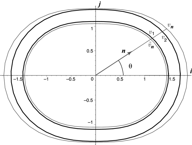
Figure 3: Polar graph of the Love wave speeds $v_{1}$ and $v_{2}$ corresponding to $kh=\pi$ as a function of the angle $\theta$ that the propagation direction $\boldsymbol{n}$ makes with the direction $\boldsymbol{i}$.

As explained in Section 5, the dispersion curves can be deduced from dispersion curves in the linear isotropic case, and are shown in Fig.2. Clearly, because $\widetilde{v}_{\boldsymbol{n}}$ varies with the chosen direction $\boldsymbol{n}$, this figure shows that the number of possible modes for a given value of the dispersion parameter $kh$ is not necessarily the same for all $\boldsymbol{n}$. We here focus on the influence of pre-strain and choose, for instance, $kh=\pi$ (wavelength equal to twice the thickness layer), a value of this parameter such that two modes of propagation are possible in all directions $\boldsymbol{n}$ : a fundamental mode with speed $v_{1}$, and a second mode with speed $v_{2}$. In Fig.3, we plot the polar graphs of $v_{\boldsymbol{n}}$, $\widetilde{v}_{\boldsymbol{n}}$, and of the Love wave speeds $v_{1}$ and $v_{2}$ of the two modes as a function of the angle $\theta$ between the propagation direction $\boldsymbol{n}$ and the principal direction $\boldsymbol{i}$, corresponding to the greatest stretch $\widetilde{\lambda}_{1}=\lambda_{1}=1.45$. We note that the greatest and least values of $v_{1}$ and $v_{2}$ correspond to propagation along the directions of greatest and least stretch in the interface, indicating an experimental way of determining these directions.

8 Conclusion

In this paper, we have obtained an exact finite-amplitude Love wave solution for a layer and a subtrate consisting of pre-strained compressible neo-Hookean materials. The dispersion relation is similar to that of linear isotropic elasticity, but an explicit dependence on the pre-strain is exhibited. In particular, the number of wave modes for different values of the dispersion parameter $kh$ ($k$: wave number, $h$: thickness of the deformed layer) is influenced by the pre-strain.

It should be emphasized that the existence of this Love wave solution is subjected to the condition that the propagation direction $\boldsymbol{n}$ and the normal $\boldsymbol{m}$ to the interface are such that $\boldsymbol{n}\boldsymbol{B}\boldsymbol{m}=\boldsymbol{n}\widetilde{\boldsymbol{B}}\boldsymbol{m}=0$, where $\boldsymbol{B}$ and $\widetilde{\boldsymbol{B}}$ are the left Cauchy-Green strain tensors characterizing the pre-strain of the subtrate and of the layer, respectively. Note that it follows from the continuity of the traction at the interface that the conditions $\boldsymbol{n}\boldsymbol{B}\boldsymbol{m}=0$ and $\boldsymbol{n}\widetilde{\boldsymbol{B}}\boldsymbol{m}=0$ are equivalent.

Thus, the interface may be arbitrarily chosen. However, when it is not a principal plane of $\boldsymbol{B}$ and $\widetilde{\boldsymbol{B}}$, there is only one propagation direction satisfying these conditions. In contrast, when the interface is a principal plane of $\boldsymbol{B}$ and $\widetilde{\boldsymbol{B}}$, all propagation directions $\boldsymbol{n}$ in this interface are possible. In this case, for a given value of $kh$, the number of possible modes is not necessarily the same for all propagation directions.

The energy flux and energy density of the solution in the layer and in the substrate have been studied in detail. In particular, it has been shown that the mean energy fluxes in the layer and in the substrate are both along $\boldsymbol{B}\boldsymbol{n}=\widetilde{\boldsymbol{B}}\boldsymbol{n}$, thus along the same direction, parallel to the interface. The fact that this direction is not along the propagation direction (except when $\boldsymbol{n}$ is a principal direction) is due to the anisotropy induced by the pre-strain.

Appendix A Uniqueness for the determination of $J$ in the substrate

Here we consider the equation (4.9) for the detemination of $J$ in the substrate when the strain tensor $\widetilde{\boldsymbol{B}}$ in the layer is given. It may also be written as

$$f(J)\equiv\textstyle{\frac{1}{2}}G^{\prime}(J)+\mu J\widetilde{J}^{-2}\boldsymbol{m}\cdot\widetilde{\boldsymbol{B}}\boldsymbol{m}=\boldsymbol{m}\cdot\widetilde{\boldsymbol{T}}\boldsymbol{m},$$ (A.1)

where $\widetilde{\boldsymbol{T}}$ is the stress tensor in the layer, corresponding to the strain tensor $\widetilde{\boldsymbol{B}}$.

First, using the strong ellipticity conditions (2.6), we note that

$$f^{\prime}(J)=\textstyle{\frac{1}{2}}G^{\prime\prime}(J)+\mu\widetilde{J}^{-2}\boldsymbol{m}\cdot\widetilde{\boldsymbol{B}}\boldsymbol{m}>0,$$ (A.2)

so that $f(J)$ is strictly monotonous increasing for $J\in[0,\infty]$. Then, recalling $G^{\prime}(1)=-2\mu$, we have $\textstyle{\frac{1}{2}}G^{\prime}(J)\leq-\mu$ for $J\leq 1$, and $\textstyle{\frac{1}{2}}G^{\prime}(J)\geq-\mu$ for $J\geq 1$, hence

$$\lim_{J\rightarrow 0}f(J)=\textstyle{\frac{1}{2}}\displaystyle\lim_{J\rightarrow 0}G^{\prime}(J)\leq-\mu,\qquad\lim_{J\rightarrow\infty}f(J)=\infty.$$ (A.3)

Owing to the monotonicity of $f(J)$, the limit for $J\rightarrow 0$ exists and is either finite and negative or $-\infty$.

If $\textstyle{\frac{1}{2}}\lim_{J\rightarrow 0}G^{\prime}(J)=-T_{0}\leq-\mu<0$ (with $T_{0}$ finite), then, clearly, for any strain tensor $\widetilde{\boldsymbol{B}}$ such that $\boldsymbol{m}\cdot\widetilde{\boldsymbol{T}}\boldsymbol{m}>-T_{0}$, equation (A.1) has exactly one solution for $J>0$. However, for any strain tensor $\widetilde{\boldsymbol{B}}$ such that $\boldsymbol{m}\cdot\widetilde{\boldsymbol{T}}\boldsymbol{m}\leq-T_{0}$, this equation has no solution for $J>0$.

If $\lim_{J\rightarrow 0}G^{\prime}(J)=-\infty$, then, clearly, whatever be the value of $\boldsymbol{m}\cdot\widetilde{\boldsymbol{T}}\boldsymbol{m}$, equation (A.1) has exactly one solution for $J>0$.

References

[1]
A.E.H. Love,
Some Problems of Geodynamics
(Dover, New York, 1967).
[2]
C. Lardat, C. Maerfeld, and P. Tournois,
Theory and performance of acoustical dispersive surface wave
delay lines,
Proc. IEEE59 (1971) 355–368.
[3]
J.T. Wilson,
Surface waves in a heterogeneous medium,
Bull. Seism. Soc. Am.32 (1942) 297–304.
[4]
H. Deresiewicz,
A note on Love waves in a homogeneous crust overlying an
inhomogeneous stratum,
Bull. Seism. Soc. Am.52 (1962) 639–645.
[5]
S.N. Bhattacharya,
Exact solutions of SH wave equation for inhomogeneous media,
Bull. Seism. Soc. Am.60 (1970) 1847–1859.
[6]
J.L. Bleustein,
A new surface wave in piezoelectric materials,
Appl. Phys. Lett.13 (1968) 412–413.
[7]
Yu. V. Gulyaev,
Electroacoustic surface waves in piezoelectric materials,
JETP Lett.9 (1969) 37–38.
[8]
B. Collet and M. Destrade,
Piezoelectric Love waves on rotated Y-cut mm2 substrates,
IEEE Trans. Ultras. Ferro. Freq. Control53 (2006) 2132–2139.
[9]
G.A. Maugin,
Elastic surface waves with transverse horizontal polarization,
Adv. Appl. Mech.23 (1983) 373–434.
[10]
M.A. Hayes and R.S. Rivlin,
Surface waves in deformed elastic materials,
Arch. Rational Mech. Analysis,
8 (1961) 358–380.
[11]
A.J. Willson,
Love waves and primary stress,
Bull. Seism. Soc. Am.65 (1975) 1481–1486.
[12]
B.K. Kar and A.K. Pal,
On the possibility of Love wave propagation under initial shear stress,
Proc. Indian natn. Sci. Acad.51 (1985) 686–688.
[13]
M.A. Dowaikh,
On SH waves in a pre-stressed layered half-space for an
incompressible elastic material,
Mech. Research Comm.26 (1999) 665–672.
[14]
G.A. Maugin,
Nonlinear Waves in Elastic Crystals
(University Press, Oxford, 1999).
[15]
A.N. Norris,
Finite amplitude waves in solids,
In: M.F. Hamilton and D.T. Redstock (eds.)
Nonlinear Acoustics
(Academic Press, San Diego, 1999) pp. 263–277.
[16]
E.A. Zabolotskaya,
Sound beams in a nonlinear isotropic solid,
Sov. Phys. Acoust.32 (1986) 296–299.
[17]
M. Destrade,
Finite-amplitude inhomogeneous plane waves in a deformed Blatz-Ko material,
in Proceedings of the 1st Canadian Conference on Non Linear
Solid Mechanics,
ed., E.M. Croitoro,
University of Victoria Press,
1 (1999) 89–98.
[18]
E. Rodrigues Ferreira and Ph. Boulanger,
Finite-amplitude damped inhomogeneous waves in a deformed Blatz-Ko material,
Math. Mech. Solids10 (2005) 377–387.
[19]
E. Rodrigues Ferreira and Ph. Boulanger,
Superposition of transverse and longitudinal
finite-amplitude waves in a deformed Blatz-Ko material,
Math. Mech. Solids12 (2007) 543–558.
[20]
M. Hayes,
A remark on Hadamard materials,
QJMAM21 (1968) 141–146.
[21]
Y. Başar and D. Weichert,
Nonlinear Continuum Mechanics of Solids
(Springer, New York, 2000).
[22]
M. Levinson and I.W. Burgess,
A comparison of some simple
constitutive relations for slightly compressible rubber-like materials,
Int. J. Mech. Sc.13 (1971) 563–572.
[23]
M.A. Biot,
Mechanics of Incremental Deformations
(John Wiley, New York, 1963).
[24]
I. Tolstoy,
Wave Propagation
(McGraw-Hill, New York, 1973).
[25]
P. Chadwick,
Continuum Mechanics
(Dover, New York, 1999).
[26]
M. Hayes,
Energy flux for trains of inhomogeneous plane waves,
Proc. R. Soc. A,
370 (1980) 417–429.
[27]
Ph. Boulanger, M. Hayes and C. Trimarco,
Finite-amplitude plane waves in deformed Hadamard materials,
Geophys. J. Int.118 (1994) 447–458.
[28] P.J. Blatz and W.L. Ko,
Application of finite elasticity to the deformation of rubbery materials.
Trans. Soc. Rheology, 6, (1962) 223–251.
[29]
W.M. Ewing, W.S. Jardetzky amd F. Press,
Elastic Waves in Layered Media
(McGraw-Hill, Nwe york, 1957).