Lifetime measurements of the $5d$ states of rubidium

Abstract

We present lifetime measurements of the $5D_{3/2}$ and $5D_{5/2}$ states of rubidium using the time correlated single photon counting method. We perform the experiment in a magneto-optical trap of ⁸⁷Rb atoms using a two-step excitation with the trap laser at 780 nm as the first step. We record the 761.9 nm fluorescence from the decay of the $5D_{3/2}$ state to the $5P_{1/2}$ state, and measure the lifetime of the $5D_{3/2}$ state $\tau=246.3(1.6)$ ns. We record the 420.2 nm fluorescence from the cascade decay of the $5D_{5/2}$ state to the $5S_{1/2}$ state through the $6P_{3/2}$ state, and extract the lifetime of the $5D_{5/2}$ state ${\tau}=238.5(2.3)$ ns.

I Introduction

Lifetime measurements are fundamental for the understanding of atomic structure. The precisely measured quantities of transition energies and excited state lifetimes are important tests of atomic structure theory through comparisons with the values derived from the calculated energies and transition matrix elements Safronova and Johnson (2008). Alkali atoms and alkali-like ions are the benchmark systems where measurements and calculations have reached the highest development because the simple single-core electron structure facilitates the application of advanced calculation methods and current simple laser cooling techniques.

A large number of lifetime measurements exist in the alkali atoms and alkali-like ions for the $s$ and $p$ levels, but there are not as many high precision measurements on the $d$ and higher angular momentum states. These states are becoming important not only in the study of fundamental symmetries Ginges and Flambaum (2004); Fortson (1993); Dzuba et al. (2001); Kreuter et al. (2005), but also in quantum information science as they are used for qubit manipulation in ion traps Steane (1997); Nägerl et al. (2000).

The $d$ states of rubidium are interesting from the calculation point of view as they remain in the domain of non-relativistic physics, but they are thoroughly affected by correlation corrections. Safronova et al. Safronova et al. (2004) have shown the important role of high order corrections, up to third order, in calculations that use many body perturbation theory (MBPT) of lifetimes of these states. We present in this paper a precise measurement of the $5D_{3/2}$ and $5D_{5/2}$ states of rubidium. Our group has studied the equivalent states in francium, the heaviest alkali atom, and achieved precisions of 0.4% and 4.3% for the $7D_{3/2}$ and $7D_{5/2}$ states, respectively Grossman et al. (2000).

Previous experimental work on the lifetime of the Rb $5D_{3/2}$ state Tai et al. (1975) and the whole $5d$ manifold Marek and Munster (1980) achieved a precision long surpassed by atomic calculations. This paper shows an improvement by more than a factor of twenty in the precision of the $5D_{3/2}$ state lifetime measurement and a precise determination of the $5D_{5/2}$ state lifetime. These improvements will hopefully trigger improved calculations as the precision of this work ($\sim 1\%$) is better than the current estimates in the theory ($\sim 5\%$) Safronova et al. (2004).

This paper has five sections. Sec. II presents the theoretical background. Sec. III explains the experimental method and apparatus. Sec. IV and V presents the data analysis for the measurements of the $5D_{3/2}$ and $5D_{5/2}$ state lifetimes, respectively. Sec. VI gives a conclusion.

II Theoretical background

Suppose an atom is in an excited state $|{e}\rangle$, and it decays to a set of lower states $\{|{l_{j}}\rangle\}$, the lifetime of this excited state, $\tau_{e}$, is Safronova et al. (2004)

$$\frac{1}{\tau_{e}}=\sum_{j}\frac{4}{3}\frac{\omega^{3}_{el_{j}}}{c^{2}}\alpha\frac{|\langle{J_{e}}||\bm{r}||{J_{l_{j}}}\rangle|^{2}}{2J_{e}+1},$$ (1)

where $c$ is the speed of light, $\hbar\omega_{el_{j}}$ is the transition energy between $|{e}\rangle$ and $|{l_{j}}\rangle$, $\alpha$ is the fine structure constant, $J$ is the angular momentum associated with each state, and $\langle{J_{e}}||\bm{r}||{J_{l_{j}}}\rangle$ is the reduced transition matrix element.

Equation (1) shows that lifetime measurements probe the overlap of wavefunctions of electron states with different quantum numbers at large distance. This is in contrast with precise energy measurements which probe the overall distribution of electron wavefunction, or the hyperfine splittings that are sensitive to the short range of the electronic wavefunctions.

Theoretical calculations aim to first find out the correct set of eigenfunctions of the atomic system Hamiltonian, and then calculate the physical properties using those results. In relativistic many-body calculations, there are different methods to obtain the eigenfunctions of the system. The most straightforward way is to start with a Dirac-Hartree-Fock (DHF) wavefunction ($|{\psi^{(0)}}\rangle$) and iterate the perturbation theory order by order. This is the relativistic many-body perturbation theory. This method usually stops at the third order due to the large calculation load. This limits the precision of the results that can also suffer when the mean field ground state is not a good starting point. An improvement is to use a wavefunction including some excitations to the DHF wavefunction Safronova and Johnson (2008):

$$|{\psi}\rangle=(1+S_{1}+S_{2}+S_{3}+\ldots)|{\psi^{(0)}}\rangle,$$ (2)

where $|{\psi^{(0)}}\rangle$ is the DHF wavefunction and $S_{i}$ is the $i$-body excitation operator. The method involving only $S_{1}$ and $S_{2}$ operators in Eq. (2) is the singles-doubles (SD) method. The so-called all-order method includes $S_{1}$, $S_{2}$ and the dominant parts of the $S_{3}$ (see Ref. Safronova et al. (1999) for an extended explanation of the method).

The calculation of transition matrix elements limits the precise prediction of the lifetimes. For the all-order method, this problem becomes serious for some levels with large correlation effects (such as $d$ levels), where the wavefunction in the form of Eq. (2) is a bad starting point of calculations. Theorists use a semi-empirical scaling scheme for certain wavefunction coefficients to solve the problem. For the rubidium $5d$ states, the lifetimes calculated with and without scaling have a relative difference of 20%, but it is hard to assert the correctness of the scaling due to high uncertainties of past experimental results Safronova et al. (2004).

Lifetime measurements help on the extraction of transition matrix elements. If there is only one decay channel, we can extract the absolute value of the reduced transition matrix element directly from the lifetime data. For example, by measuring the lifetimes of the excited states, Ref. Simsarian et al. (1998) extracts the transition matrix elements $|\langle{7P_{1/2}}||r||{7S_{1/2}}\rangle|$ and $|\langle{7P_{3/2}}||r||{7S_{1/2}}\rangle|$ of Fr, and Ref. Hoeling et al. (1996) extracts the transition matrix element $|\langle{5D_{5/2}}||r||{6P_{3/2}}\rangle|$ of Cs. The case of a multi-channel decay sometimes requires a combination of various experimental approaches to extract the transition matrix elements Safronova and Johnson (2008), including the measurement of static scalar polarizability Arora et al. (2007), and nonresonant two-photon, two-color linear depolarization spectrum Bayram et al. (2000).

III Experimental method and setup

We adapt the time correlated single photon counting method O’Connor and Phillips (1984) in this experiment with a cold sample of ⁸⁷Rb atoms (temperature less than 100 $\mu$K) in a magneto-optical trap (MOT). After exciting the atoms to the $5d$ states, we turn off the excitation beams and record the delay between the fluorescence and a fixed time reference. Here, the single photon counting technique refers to the fact that we record at most one photon in one duty cycle. It is possible for the detector to detect more than one photon in one cycle, but once the electronics record one signal, they will not accept another until a new cycle begins. This method works best when the probability of detecting more than one photon in one cycle is very small, which in turn keeps the corrections low (see the pulse pileup corrections in the systematic study of Sec. IV). In our experiments, we detect one photon in about one hundred cycles.

We use a rubidium dispenser as the atomic vapor source and the MOT resides inside a 15 cm radius spherical chamber with the vacumm pressure of $10^{-10}$ Torr. A pair of anti-Helmholtz coils provides a magnetic gradient of 6 G/cm and three pairs of Helmholtz coils provide the fine tuning of the magnetic environment. A Coherent 899-01 Ti:Sapphire laser with linewidth better than 100 kHz provides three pairs of MOT trapping beams with intensity of 8 mW/cm², and the laser is red detuned from the $5S_{1/2},F=2$ $\rightarrow$ $5P_{3/2},F=3$ transition by approximately 20 MHz. A Toptica SC110 laser provides the repumper beam with intensity of 3 mW/cm² and it is on resonance with the transition $5S_{1/2},F=1$ $\rightarrow$ $5P_{3/2},F=2$. We capture about $10^{5}$ atoms in the MOT with diameter of 600 $\mu$m and peak density of around $10^{9}$ cm^-3. We use two charge-coupled device (CCD) cameras to monitor the fluorescence of the MOT in two perpendicular directions.

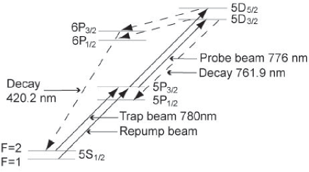
Figure 1: ⁸⁷Rb energy levels involved in the experiment.

We list the relevant energy levels of ⁸⁷Rb for this experiment in Fig. 1. We use a two-step transition to reach the $5d$ states, where the trapping beam of the MOT enables the first step and the $5P_{3/2},F=3$ state is the intermediate state. A SDL TC40-D laser with linewidth of 5 MHz provides the probe beam to reach the 5$d$ states. We inject the probe beam to the MOT region through a single mode fiber, which sets the waist ($1/e^{2}$ power) to 1.2 mm. The power of the probe beam is 0.5 mW for the excitation to the $5D_{5/2},F=4$ state, and 1.0 mW for the excitation to the $5D_{3/2},F=3$ state.

We lock the frequency of the trapping beam using the Pound-Drever-Hall method with saturation spectroscopy in a Rb cell. We send part of the frequency modulated light employed on this lock to an independent rubidium glass cell, where this light overlaps with a small laser beam taken from the probe beam. We monitor the absorption of the 780 nm light as a function of the frequency of the 776 nm laser, and the intermodulation of the sidebands yields error-signal like features that we use to lock the frequency of the probe beam on resonance A. Pérez Galván et al. (accepted by Can. J. Phys.); Boucher et al. (1992).

We use a cycle of 10 $\mu$s length, and have two different schemes for photon detection and time control for the two different measurements. In the $5D_{3/2}$ state lifetime measurement, we put a 760 nm interference filter with bandwidth of 10 nm (Andover 760FS10-25) in front of the detector, a Hamamatsu R636 photomultiplier tube (PMT) with quantum efficiency of 10% at this wavelength. Since a large amount of 780 nm photons from the scattered trapping beam pass through the filter, we turn the trapping beam off after the excitation phase to decrease the background. We use two acousto-optical modulators (AOM) to turn on and off the trapping beam and the probe beam. In the $5D_{5/2}$ state lifetime measurement, we use a 420 nm interference filter with a bandwidth of 10 nm (Andover 420FS10-25) in front of the detector, a PerkinElmer C962 channel PMT with quantum efficiency of 15% at this wavelength. The trapping beam has a negligible contribution to the background in this case. We use a Gsänger LM0202P electro-optical modulator (EOM) and an AOM to chop the probe beam for this experiment. The turn off ratio of EOM and AOM is better than 30:1 in 30 ns. Fig. 2 shows the time sequence of the pulses.

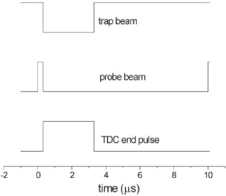
Figure 2: Time sequences in the lifetime measurement. Each cycle has a period of 10 $\mu$s.

The PMT is about 35 cm away from the MOT and we use a 10X Computar Macro Zoom lens in front of it for light collection. Two synchronized Stanford Research DG535 pulse generators, which have a 5 ps delay resolution and 50 ps rms jitter, provide all the time references in the signal process. The signal from the PMT goes through the amplifiers first. In the $5D_{3/2}$ ($5D_{5/2}$) lifetime measurement, we amplify the signal from the Hamamastsu R636 PMT (channel PMT) 64 (4) times using an EG&G AN106/n plus an AN101/n DC amplifier (an AN106/n amplifier alone). The output goes through an Ortec 583 constant fraction discriminator (CFD) and a Lecroy 7126 level translator. The level translator converts the input signal to ECL, TTL and NIM outputs. We send the output of the NIM signal to a Stanford Research SR430 multi-channel scaler to monitor the photon counting histogram during the experiment. We send the ECL signal as a start pulse to a Lecroy 3377 time-to-digital converter (TDC), which has a resolution of 0.5 ns and is triggered by the falling edge of the input pulse. The TDC measures the delay between the observed photon and the fixed pulse given by the pulse generator (see Fig. 2 and Fig. 3). The output of the TDC goes to a Lecroy 4302 memory and we read out the results through a Lecroy 8901A GPIB interface. Fig. 3 shows the diagram of the signal process.

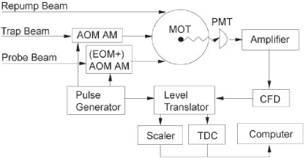
Figure 3: The setup of the detection and signal process.

IV Lifetime of the $5D_{3/2}$ state

We excite the atoms to the $5D_{3/2}$ state and about 50% of the atoms decay into the $5P_{1/2}$ state with fluorescence at 761.9 nm, where we get the branching ratios using the transition matrix elements from Ref. Safronova et al. (2004). We record the fluorescence and accumulate data until the peak count is more than 1000 for each data set. This usually takes half an hour to 45 minutes. The ratio of peak signal to background is generally around 40, and we take an additional data set of background for roughly the same time. The upper plot of Fig. 4 shows a typical data set after substraction of background. There is another possible way to observe the decay through the detection of 420 nm fluorescence that comes from the $6p$ manifold (see Fig. 1). This has a great background advantage, but requires fitting to a sum of three exponentials, which challenges our fitting process (see explanations in the Sec. V). The results that we present here are consistent with a preliminary analysis of the blue decay.

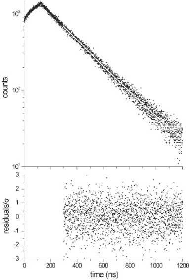
Figure 4: Upper plot: time distribution of 761.9 nm photons (black points) in the measurement of the $5D_{3/2}$ state with the fitting function (white line). Lower plot: normalized fit residuals. We have subtracted the background in the decay curve and we use the statistical error of the data to normalize the fit residuals.

IV.1 Decay model

The data in Fig. 4 shows an increase of the fluorescence due to the excitation of the system by the probe beam and the decay after turning off the probe beam. We qualitatively understand the rising part by treating this many-level system as a four-level system. We denote the ground state, the $5P_{3/2}$ state and the $5D_{3/2}$ state as levels 1, 2 and 3, and treat all other states that the $5D_{3/2}$ state decays to as level 4. The excitation rate from level $i$ to $j$ is $A_{ij}$, the spontaneous decay rate of level $k$ is $R_{k}$ and the branching ratio of decay channel from $k$ to $l$ is $\gamma_{kl}$. Because the system is already in the steady state before we turn on the weak probe beam, we take the second step transition as a small perturbation to the system and get the rate equations:

$$\dot{N}_{3}=A_{23}N_{2}-R_{3}N_{3}$$

$$\dot{N}_{4}=\gamma_{34}R_{3}N_{3}-R_{4}N_{4}.$$ (3)

The initial condition is $N_{1}(0)=N_{2}(0)=N_{0}/2$, where $N_{0}$ is the total number of atoms and the time origin is the time we turn on the probe beam. This gives the number of atoms in level 3 as

$$N_{3}(t)=\frac{A_{23}}{R_{3}}\frac{N_{0}}{2}[1-\exp{(-R_{3}t)}],t<t_{1},$$ (4)

where $t_{1}$ is the time we turn off the probe beam. This qualitatively agrees with the rising behavior of the signal.

The number of atoms in this level begins to decay when we turn off the probe beam. For a perfect turnoff at time $t_{1}$, we get the decaying behavior:

$$N_{3}(t)=N_{3}(t_{1})\exp{[-R_{3}(t-t_{1})]},t>t_{1}.$$ (5)

The intensity of the fluorescence from the $5D_{3/2}$ state to the $5P_{1/2}$ state is proportional to the atom number in the $5D_{3/2}$ state and Eq. (5) shows that the decaying part of the signal is independent of the excitation part except for a coefficient.

IV.2 Fitting process

We use the Levenberg-Marquardt (L-M) algorithm Press et al. (1987) and fit the data to the function

$$y=A{\exp}(-t/\tau)+B,$$ (6)

where the $\tau$ is the $5D_{3/2}$ state lifetime and B describes the background. The fitting is a procedure to minimize $\chi^{2}$:

$$\chi^{2}=\displaystyle\sum_{i}\omega_{i}(y_{i}-y_{f})^{2},$$ (7)

where $y_{i}$ and $y_{f}$ are the experimental and fitting value for the $i$th data point, and $w_{i}$ is the inverse of the square of the statistical error of the data assuming the data follow the Poisson distribution.

We use two criteria on the choices of the range of the data to fit. First, we choose the starting point of the fitting range away from the turning off point to avoid pulse turnoff effects. Second, we need to make sure that the fitting results are stable when we vary the starting and end points of the fitting range. This fitting process gives us an average of reduced $\chi^{2}=1.03$ for all the data sets we have taken. The lower plot of Fig. 4 shows the normalized fit residuals of the upper plot data.

IV.3 Statistical error

We have taken 28 sets of data with the same experimental conditions, with each individual data set fitting error, $\sigma_{i}$, of around 1%. Considering this sample of 28 data points, we obtain a weighted mean lifetime of 246.5 ns, with the error given by $({\sum{1/\sigma_{i}^{2}}})^{-1/2}$, which is 0.3 ns. We choose to scale the uncertainty by a factor Yao et al. (2006)

$$S=\left[{\chi^{2}/(N-1)}\right]^{\frac{1}{2}},$$ (8)

where $\chi^{2}$ is defined in Eq. (7), and $N$ is the number of data points. In this way, the mean value does not change, but it helps to solve the problem of underestimation of the error on some data sets. We get $S=2.1$, and the statistical error as 0.6 ns.

IV.4 Systematic effects

We focus on the following systematic effects:

Time calibration and height nonuniformity of TDC. We send two pulses with a fixed delay from the DG535 pulse generator as the start and end pulses to the TDC. By comparing the readout of the TDC with the calibrated delay, we get a nonlinearity of the TDC time calibration of less than 0.01%, which in turn gives an error on the lifetime measurement of less than 0.01%. To check the height uniformity of the TDC channels, we change the source of the photon to the scattering of laser light on a paper. We control the power of the laser so that the recording rate is similar to that in the lifetime experiments, and accumulate data until the count of each channel reaches 100. We fit the results with a linear function (fits to higher order polynomials yield the same conclusion) and get a slope of 0.1 count per 1000 channels, which gives an error of 0.01% on the lifetime measurement.

Pulse pileup correction. There is a difference between the number of the signals detected and signals recorded in the single photon counting method, this leads to pulse pileup correction. Suppose we have $N_{E}$ cycles of excitation, and get $N_{j}$ counts on the $j$th channel of the TDC, then the pulse pileup corrected result of the $i$th channel is

$$N_{i}^{\prime}=\frac{N_{i}}{1-\frac{1}{N_{E}}\displaystyle\sum_{j<i}N_{j}}.$$ (9)

This gives us a correction of around -0.1% for our measurements.

Quantum beats. Quantum beats come from the interference of the decay paths from several coherently excited states to the same lower state. By considering this effect, we rewrite the Eq. (6) as Demtröder (1996)

$$y=A\exp(-t/\tau)[1+\displaystyle\sum_{i}C_{i}\cos(\omega_{i}{t})]+B,$$ (10)

where the sum is over all possible interference paths and $\hbar\omega_{i}=\Delta{E_{i}}$ is the energy difference of two excited states involved in the process. This has been an important issue when the probe beam has a large bandwidth Young et al. (1994).

We first consider the possibility of the quantum beats from the hyperfine structure. The energy difference between $5D_{3/2},F=2$ and $F=3$ sates is around 40 MHz Tai et al. (1975). This separation is much larger than the probe laser linewidth. The natural linewidth of the $5D_{3/2}$ state is 0.6 MHz, considering the power broadening effect, the transition linewidth is at most 6 MHz. A sharp turnoff process could generate a large bandwidth in frequency domain. We decompose the probe pulse in frequency range by the fast Fourier transform (FFT), and find that the high frequency components (higher than 40 MHz) only take about $1/200$ of the total power. In conclusion, the probability to coherently excite the hyperfine states is negligible. The FFT of the fitting residuals does not show any peaks around the frequency of the hyperfine splitting either.

We position the atoms at the zero of the magnetic field in the MOT, but the finite extent of the cloud sample regions with a magnetic field. The Zeeman splitting introduced by this magnetic field could be a source of quantum beats, because we always leave the gradient magnetic field for the MOT on during the experiment. However, the overlapped $\sigma+$ and $\sigma-$ trapping beams tend to average out this effect.

We estimate an upper bound of the effect due to the Zeeman splitting following the treatment in Ref. Grossman et al. (2000). We have $\hbar\omega=\Delta{m_{F}}g_{F}\mu_{B}{B}$, where $\Delta{m_{F}}=2$, $g_{F}=0.4$ for $5D_{3/2},F=3$ state, and $\mu_{B}$ is the Bohr magneton. The size of the MOT is around 600 $\mu$m and the magnetic gradient is around 6 G/cm, we use the maximum magnetic field 0.18 G in that region for the calculation. This gives us a maximum beat frequency of 202 kHz, which sets an upper bound of this error of 0.15%.

We also look for possible effects of the magnetic field by changing the magnetic field gradient from 5 G/cm to 10 G/cm and do not find any systematic changes. Fig. 5 shows the results, where the smaller error bars in the points with 4.9 G/cm and 9.8 G/cm are due to more data sets under those conditions in this systematic study. Studies of linear correlation coefficient of the data points show that they are highly uncorrelated. We get an error of 0.16% by this effect, which is the standard deviation of the data points taken in this study. We use this measured bound of 0.16% for possible magnetic effects that include the quantum beats.

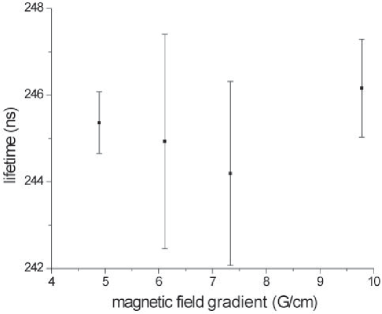
Figure 5: The systematic study of the effect of the magnetic field gradient on the $5D_{3/2}$ lifetime measurement.

Radiation trapping. Radiation trapping comes from the reabsorption of the emitted photon by the sample itself. This effect depends on the length and density of the sample and could increase the measured lifetime substantially when there are many atoms Gomez et al. (2005). The MOT has the advantage of its size, which makes this effect much smaller compared with the experiment in the cell. Denote $l$ and $n$ as the length and density of the sample, and $\alpha$ as the atomic absorption coefficient. Ref. Kibble et al. (1967) gives an expression for this effect:

$$\frac{\tau^{\prime}}{\tau}=1+\left(\frac{C}{\lambda}\right)^{2},$$ (11)

where $C=l{\alpha}n$ and $\lambda\tan(\lambda)=C$. In the limit of small length, Eq. (11) becomes

$$(\tau^{\prime}-\tau)={\tau}C={\tau}l\alpha{n},$$ (12)

where the change of lifetime depends linearly on density. We have changed the density of our sample by a factor of six to look for this effect, and do not observe any systematic changes. The error due to this effect is smaller than 0.1%.

Other systematics. The pulse length and power of the probe beam are the parameters controlling the number of atoms in the excited states. By changing the pulse length from 320 ns to 720 ns, and also the power from 0.5 mW to 2.4 mW, we do not observe systematic changes. We set the error on those effects as 0.6%, which we obtain in the same sprit as in the study of the magnetic field effects.

IV.5 Summary and comparison

We list the error budget of the $5D_{3/2}$ lifetime measurement in table 1, and compare our result with the previous experimental and theoretical work in table 2. On the experimental part, Ref. Tai et al. (1975) made use of the Hanle effect to extract the lifetime. In that case, they could not optically excite the atoms to the $5D_{3/2}$ state, instead, they optically excited the atoms to a higher $p$ state and populated the desired level by spontaneous emission. On the theoretical part, Ref. Theodosiou (1984) used the quantum defect theory with a realistic potential, and Ref. Safronova et al. (2004) used the scaled all-order method.

The result of Ref. Safronova et al. (2004) sits on the edge of 2$\sigma$ range of our data and that of Ref. Theodosiou (1984) sits on the edge of the 4$\sigma$ range. For more detailed comparison, we need to know the range of validity of the theoretical calculation. A possible way to define the error of the all-order method calculation is comparing its results with third order many body perturbation theory. In this way, the error of the all-order method calculation for the Rb $5d$ states lifetime is around 5% Safronova (private communication), and our result of the $5D_{3/2}$ state lifetime stays within its prediction. Our result $1\sigma$ range has a small overlap with the $1\sigma$ range of the result of Ref. Tai et al. (1975), which has a much bigger error bar.

Table 1: Error budget of the $5D_{3/2}$ state lifetime measurement.

Source	Correction (%)	Error(%)
Statistical		$\pm$0.25
Time calibration		$<\pm$0.01
TDC nonuniformity		$\pm$0.01
Pulse pileup	-0.1
Quantum beats and magnetic field		$\pm$0.16
Radiation trapping		$<\pm$0.10
Other Systematics		$\pm$0.60
Total		$\pm$0.66

Table 2: Comparison of the measured lifetime of the $5D_{3/2}$ state with the previous work.

		$\tau_{5D_{3/2}}$ (ns)
Experiment	This work	246.3$\pm$1.6
	Tai et al. Tai et al. (1975)	205$\pm$40
Theory	Theodosiou Theodosiou (1984)	240
	Safronova et al. Safronova et al. (2004)	243

V Lifetime of the $5D_{5/2}$ state

About 30% of the atoms in the $5D_{5/2}$ state decay to the $6P_{3/2}$ state with fluorescence at 5 $\mu$m, and about 25% of the atoms in the $6P_{3/2}$ state decay to the ground state with fluorescence at 420.2 nm, where we get the branching ratios in the same way as in Sec. IV. We record this blue fluorescence and accumulate data until the peak count is more than 1000 for each data set. The upper plot of Fig. 6 shows a typical data set. Since we detect the blue photon, the background is very small (less than 1 count per channel in half an hour), and we do not have to take an additional background data.

Most of the data process and systematic effects studies in this measurement are similar to those in the measurement of the $5D_{3/2}$ state, however, there are some new features in the analysis.

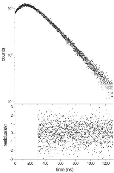
Figure 6: Upper plot: time distribution (black points) of the blue photon in the measurement of the $5D_{5/2}$ state with the fitting function (white line). Lower plot: normalized fit residues, where the normalization factor is the statistical error of the data.

V.1 Decay model

We use the same model in the previous section. The differences are that we change the $5D_{3/2}$ state to the $5D_{5/2}$ state and specify level 4 as the $6P_{3/2}$ state, because the fluorescence we observe in this experiment is proportional to number of atoms in the $6P_{3/2}$ state. Using the same notation as in Sec. IV.1, we get the rising and decaying part of the signal in this experiment as

$$N_{4}(t)= \frac{\gamma_{34}R_{3}}{R_{4}-R_{3}}\frac{A_{23}N_{0}}{2}$$

$$\left[\frac{1-\exp(-R_{3}t)}{R_{3}}-\frac{1-\exp(-R_{4}t)}{R_{4}}\right],t<t_{1}$$

$$N_{4}(t)= \left[N_{4}(t_{1})-\frac{\gamma_{34}R_{3}}{R_{4}-R_{3}}N_{3}(t_{1})\right]\exp{[-R_{4}(t-t_{1})]}$$ (13)

$$+\frac{\gamma_{34}R_{3}}{R_{4}-R_{3}}N_{3}(t_{1})\exp{[-R_{3}(t-t_{1})]},t>t_{1}$$

This shows that the curve observed in this experiment includes the information of the lifetimes of the $5D_{5/2}$ state and the $6P_{3/2}$ state.

V.2 Fitting process

The ratio between coefficients of the two exponentials depends on the lifetimes and initial atom number at the turnoff point of both states (see Eq. (13)). If we want to fit the decay curve according to the function in Eq. (13), we have to evaluate the atom number by doing the convolution of the excitation pulse with the formula that determines population in the $6P_{3/2}$ state. A simple way to avoid this process is to leave both coefficients as free parameters and fit the decay signal away from the turnoff point Gomez et al. (2005). The existence of a stable range of fitting results when we change the starting and end points of the fitting range is a test of the validity of this treatment.

We use the following fitting function to describe the data

$$y=A_{1}\exp(-t/\tau_{5D_{5/2}})+A_{2}\exp(-t/\tau_{6P_{3/2}})+B,$$ (14)

where $\tau_{5D_{5/2}}$ and $\tau_{6P_{3/2}}$ are the lifetimes of the $5D_{5/2}$ and $6P_{3/2}$ states, respectively and B is a possible background.

If we leave both lifetimes as free parameters, the L-M algorithm does not give reliable results (it tends to equate both lifetimes). Therefore, we fix the value of $\tau_{6P_{3/2}}$ in the fitting process to solve this problem, and the value we use is the weighted average $\tau_{6P_{3/2}}$=112.8$\pm 1.7$ ns from previous experimental work listed in Ref. Marek and Munster (1980). Our fitting process gives an averaged reduced $\chi^{2}$ of 1.09 for all the data sets we have taken. The lower plot of Fig. 6 shows the normalized fit residuals by comparing the raw data and fit result in the upper plot.

V.3 Statistical error

We have taken 10 sets of data with the same experimental conditions, with each individual data set fitting error, $\sigma_{i}$, of around 1%. Following the same procedure in the Sec. IV, we get a weighted mean lifetime of 238.6 ns, error of the mean as 0.8 ns, and the scaling factor $S=1.2$. We choose the scaled error of the mean as the statistical error, which is 1.0 ns.

V.4 Systematic effects

We have studied all systematic effects listed in the measurement of the $5D_{3/2}$ state, which shows similar results. We focus on the following new situations in this measurement:

Quantum beats. It is possible to coherently excite the atoms to the Zeeman sublevels of the $5D_{5/2}$ state, but to observe the quantum beats signal for this cascade decay, we also need to prepare the coherence on the $6P_{3/2}$ state, for example, by means of selecting polarization on the fluorescence Aspect et al. (1984). In our experiment, we do not attempt to observe the coherence in the intermediate level, and do not expect observable quantum beats effects. We check the Fourier transform of the fitting residuals and do not find peaks. We also check the magnetic field effects on the lifetime measurement and do not see any systematic effects. We set the error as 0.44%, which is defined in same way of that in the systematic study in Sec. IV.

Bayesian error. In the fitting process, we do not treat $\tau_{6P_{3/2}}$ and $\tau_{5D_{5/2}}$ as independent parameters because we fix the $\tau_{6P_{3/2}}$ by its experimental value. Hence there is correlation between the values of $\tau_{6P_{3/2}}$ and $\tau_{5D_{5/2}}$ in the fitting process. We express the probability of finding $\tau_{5D_{5/2}}$ equal to $\tau_{1}^{\prime}$ as

$$P(\tau_{1}^{\prime})={\int}P(\tau_{1}^{\prime}|\tau_{2}^{\prime})P(\tau_{2}^{\prime})d\tau_{2}^{\prime},$$ (15)

where $\tau_{2}^{\prime}$ denotes the possible value of $\tau_{6P_{3/2}}$ and $P(\tau_{1}^{\prime}|\tau_{2}^{\prime})$ is the conditional probability of getting $\tau_{5D_{5/2}}=\tau_{1}^{\prime}$ when $\tau_{6P_{3/2}}=\tau_{2}^{\prime}$. Eq. (15) shows that the error of $\tau_{6P_{3/2}}$ value propagates to that of $\tau_{5D_{5/2}}$ value through the correlation, and this is the Bayesian error.

Following the treatment of Ref. Aubin et al. (2004), we change the value of $\tau_{6P_{3/2}}$ from 108 ns to 118 ns with an increase of 0.5 ns each step, and do the fitting process to extract a new $\tau_{5D_{5/2}}$ for each new value of $\tau_{6P_{3/2}}$. This scanning range has covered 3$\sigma$ range of the experimental result of $\tau_{6P_{3/2}}$. We find that a linear function describes well the dependance of the fitting result of $\tau_{5D_{5/2}}$ on the value of $\tau_{6P_{3/2}}$

$$\tau_{1}(\tau_{2})=\tau_{1}+\alpha(\tau_{2}^{\prime}-\tau_{2}),$$ (16)

where the notation is the same as in Eq. (15). Hence we get the Bayesian error as $|\alpha|\sigma_{\tau_{6P_{3/2}}}$. For our data sets, the analysis gives $\alpha$ as -0.3, and the Bayesian error as 0.5 ns.

Other systematics. We study the pulse length and power effects, and do not find any systematic changes in the lifetime values. The limit set on this error due to these effects is 0.73%.

V.5 Summary and Comparison

We list the error budget of the $5D_{5/2}$ state lifetime measurement in the table 3 and compare our result with the previous experimental and theoretical work in table 4. The result of Ref. Safronova et al. (2004) sits within the $2\sigma$ range of our data, and that of Ref. Theodosiou (1984) sits close to the edge of the $3\sigma$ range. Since the error of the all-order method estimation on this level is 5% (see the Sec. IV.5), the result of Ref. Safronova et al. (2004) is consistent with our result. On the experimental part, as far as we know, there has been no explicit experiment data on the $5D_{5/2}$ state lifetime.

The measurement of Ref. Marek and Munster (1980) gave a lifetime of the combination of $5D_{3/2}$ and $5D_{5/2}$ states. According to our results, the lifetime of the whole $5d$ manifold should sit between 238.5 ns and 246.3 ns, which is consistent with the result of Ref. Marek and Munster (1980).

Table 3: Error budget of the $5D_{5/2}$ state lifetime measurement.

Source	Correction (%)	Error(%)
Statistical		$\pm$0.40
Time calibration		$<\pm$0.01
TDC nonuniformity		$\pm$0.01
Pulse pileup	-0.05
Magnetic filed		$\pm$0.44
Radiation trapping		$<\pm$0.1
Bayesian		$\pm$0.21
Other Systematics		$\pm 0.73$
Total		$\pm$0.96

Table 4: Comparison of the measured lifetime of the $5D_{5/2}$ state with the previous work.

		$\tau_{5D_{3/2}}$ (ns)
Experiment	This work	238.5$\pm$2.3
	Marek and Munster Marek and Munster (1980)	230$\pm$23
Theory	Theodosiou Theodosiou (1984)	231
	Safronova et al. Safronova et al. (2004)	235

VI Conclusion

In this work, we have measured the lifetime of the Rb $5D_{5/2}$ state obtaining $\tau_{5D_{3/2}}=246.3\pm 1.6$ ns, and we have improved the precision of the $5D_{3/2}$ lifetime result, $\tau_{5D_{5/2}}=238.5\pm 2.3$ ns, by a factor of 25. Our results have enough precision to confirm the improvement of the scaled all-order method Safronova et al. (2004).

Our experimental condition present several advantages over previous experimental efforts: the new laser technique which allows us to optically excite the atoms to the desired states directly, the lock technique of both lasers in the two-step transition which makes the transition much more efficient and the use of a MOT which simplifies the systematic studies.

Our future work, the search of anapole moment in alkali atoms Gomez et al. (2007), relies on high precision atomic structure calculations to extract the fundamental information from the measurement. We hope the advance on the experimental value of the lifetime will contribute to new improvements on the precision of theoretical calculations.