Four New Stellar Debris Streams in the Galactic Halo

Abstract

We report on the detection of four new stellar debris streams and a new dwarf galaxy candidate in the Sloan Digital Sky Survey. Three of the streams, ranging between 3 and 15 kpc in distance and spanning between 37°  and 84°  on the sky, are very narrow and are most probably tidal streams originating in extant or disrupted globular clusters. The fourth stream is much broader, roughly 45 kpc distant, at least 53°  in length, and is most likely the tidal debris from a dwarf galaxy. As the streams each span multiple constellations, we extend tradition and designate them the Acheron, Cocytos, Lethe, and Styx streams. At the same distance and apparently embedded in the Styx stream is a $\sim 1$ kpc-wide concentration of stars with an apparently similar color-magnitude distribution which we designate Bootes III. Given its very low surface density, its location within the stream, and its apparently disturbed morphology, we argue that Bootes III may be the progenitor of Styx and in possibly the final throes of tidal dissolution. While the current data do not permit strong constraints, preliminary orbit estimates for the streams do not point to any likely progenitors among the known globular clusters and dwarf galaxies.

1. Introduction

Despite the once common belief that the stellar debris streams produced by tidal stripping of dwarf galaxies and globular clusters would be quickly dispersed by molecular cloud scattering, orbital precession, and phase mixing, recent observations of our Galaxy and others have shown that such streams are both common and evidently long-lived. The Sloan Digital Sky Survey (SDSS) has proven to be a particularly remarkable resource for finding such streams, and for studying Galactic structure at a level of detail which we cannot hope to match in any other galaxy. In addition to the large scale features attributed to past galaxy accretion events (Yanny et al., 2003; Majewski et al., 2003; Rocha-Pinto et al., 2004; Grillmair, 2006a; Belokurov et al., 2006b; Grillmair, 2006b; Belokurov et al., 2007), SDSS data has been used to detect the remarkably strong tidal tails of Palomar 5 (Odenkirchen et al., 2001; Rockosi et al., 2002; Odenkirchen et al., 2003; Grillmair & Dionatos, 2006a) and NGC 5466 (Belokurov et al., 2006a; Grillmair & Johnson, 2006), as well as the presumed globular cluster stream GD-1 (Grillmair & Dionatos, 2006b). Though spectroscopic follow-up and detailed numerical calculations have yet to be carried out for most of these streams, they will no doubt become important for constraining the three dimensional shape of the Galactic potential. Globular cluster streams will be particularly important since they are dynamically very cold (Combes, Leon, & Meylan, 1999) and therefore useful for constraining not only the global Galactic potential but also its lumpiness (Murali & Dubinski, 1999).

In this paper we continue our search of the SDSS database for more extended structures in the Galactic halo. We describe our analysis procedure in Section 2. We discuss four new stellar streams and a possible dwarf galaxy progenitor in Section 3 and put initial constraints on their orbits in Section 4. We make concluding remarks Section 5.

2. Data Analysis

Data comprising $g,r,$ and $i$ photometry for $7\times 10^{7}$ stars in the region $108\arcdeg~{}<\alpha<270\arcdeg~{}$ and $-4\arcdeg~{}<\delta<65\arcdeg~{}$ were extracted from the SDSS DR5 database using the SDSS CasJobs query system. The data were analyzed using the matched filter technique employed by Grillmair & Johnson (2006), Grillmair & Dionatos (2006a), Grillmair & Dionatos (2006b), Grillmair (2006a), and Grillmair (2006b), which itself is a variation on the optimal filtering technique described by Rockosi et al. (2002). This technique is made necessary by the fact that, over the magnitude range and over the region of sky we are considering, the surface densities of foreground stars are some three orders of magnitude greater than the surface densities of known stellar debris streams. Applied in the color-magnitude (CM) domain, the matched filter is a means by which we can optimally differentiate between streams and foreground populations.

Our filtering technique departs somewhat from that of Rockosi et al. (2002), who were primarily interested in searching for debris from a known and relatively well characterized progenitor. By contrast, our present goal is to survey the sky for discrete but hitherto unknown stellar populations. Since we are interested in detecting streams throughout the Galactic halo, we also need to account for the effects of survey completeness as we search larger and larger volumes. Consequently, rather than using the observed color-magnitude distribution (CMD) for stars of interest (e.g. Rockosi et al. (2002)), we generate template distributions which are based on the observed color-magnitude sequences of several globular clusters situated within the SDSS survey area. Specifically, we measure normal points lying along the $g-r$ and $g-i$ color-magnitude sequence of each cluster and then interpolate to compute the expected color at any $g$ magnitude. Using mean photometric errors as a function of magnitude (measured in relatively sparse regions of the survey area where source crowding is not an issue) we broaden the globular cluster sequences by convolving with appropriate Gaussians at each magnitude level. We also apply a fixed broadening of $\sigma=0.02$ mag at all magnitudes to account for the intrinsic spread in the colors of giant branch stars.

Since we have no a priori knowledge concerning the luminosity function of stars in streams, and since we need to decouple observed luminosity functions from the survey completeness, we adopt a general form for the luminosity function based on the very deep luminosity function of $\omega$ Cen (de Marchi, 1999), converted to the Sloan system using the empirical transformations of Jordi, Grebel, & Ammon (2006). We find that the exact form of the luminosity function is not particularly important. Experiments with the somewhat steeper luminosity functions one might expect for tidally stripped stars (Koch et al., 2004) yield no perceptible improvements over the range of absolute magnitudes considered here.

Comparing the observed luminosity function in the outskirts of M 13 with the much deeper $\Omega$ Cen luminosity function, we derive an approximate completeness function which is unity at $g=22$, 0.5 at $g=23.3$, and 0 at $g=24.4$. While the actual completeness will vary across the survey area, practical concerns require that we use a single completeness function for the entire field. Since we impose a cutoff at $g=22.5$, small modifications to the form of our completeness function have only very minor effects on the results. Our expectation is that mismatches between our template color-magnitude sequences and the largely unknown distributions of stars in stellar streams will have a much larger effect on our sensitivity to discrete populations.

Once the color-magnitude distribution of the stars of interest has been constructed, an optimal filter requires that this distribution be divided by the corresponding distribution of field stars (e.g. Rockosi et al. (2002)). We sample the field star distribution over various portions of DR5, binning the stars in $g$ and $g-i$ (or $g-r$), and then slightly smoothing over the bins with a Gaussian of kernel $\sigma=0.02$ mag. Figure 1 shows a template filter based on the CMD of M 13 at its nominal distance of 7.7 kpc (Harris, 1996). To avoid numerical issues in relatively unpopulated regions of the color-magnitude diagram, we set the filter to zero for stars more than 6$\sigma$ from the color-magnitude sequence. Examination of Figure 1 shows that the most highly weighted stars are those at the main sequence turn-off. Stars fainter and redward of the turn-off are much less favored, though their integrated contribution remains significant. By virtue of both their relatively small numbers, and of colors that are indistinguishable from the bulk of the foreground population, the subgiant and lower giant branch stars are given comparatively little weight.

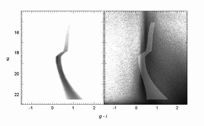
Figure 1.— Panel (a): An example of a matched filter based on the SDSS color-magnitude distribution of stars in M 13, but with a luminosity function based on $\Omega$ Cen. The stretch is logarithmic. The peak response of the filter occurs on the blue side of the main sequence turn-off, where there are relatively few foreground stars. The subgiant and lower giant branch are somewhat deweighted due to the very large number of intervening foreground stars in this color range. The width of the filter is based primarily on the mean SDSS photometric errors as a function of magnitude. Stars lying more than $6\sigma$ from the sequence are given a weight of zero. Panel (b): The color-magnitude distribution of stars lying within 10°  of the eastern half of the Cocytos stream, with the filter in panel (a) overlaid.

We used all stars with $15<g<22.5$, and we dereddened the SDSS photometry as a function of position on the sky using the DIRBE/IRAS dust maps of Schlegel, Finkbeiner, & Davis (1998). In an initial survey, a single Hess diagram for field stars was generated using roughly half the Sloan survey area in regions where no streams are currently known to exist. We applied the filters to the entire survey area, and the resulting filtered star counts were summed by location on the sky to produce two dimensional, filtered surface density maps. Once the streams were detected, we optimized the filters for individual streams. Since the CM distribution of the field star population varies over the survey area, we expect that a filter incorporating the distribution of only nearby field stars will enhance the signal-to-noise ratio of the streams. For each stream we sampled the field star population within 10°  of the stream, and with one exception, extending along only the eastern and western halves of each stream. This has the effect of increasing the measured signal-to-noise ratio by a few percent beyond what one can achieve using a single, survey-wide field star distribution. Panel (b) of Figure 1 shows an example of one such field star distribution. Further improvements may be possible by more finely subdividing the field star populations, or modeling the foreground population as a function of sky position, but that is beyond the scope of this paper.

In Figure 2 we show the filtered star count distributions after shifting the optimal filters by -1.4, +0.6, +1.2 (M 13-based filter) and +3.2 mags (M 15-based filter). The field area is shown in the Sloan Survey coordinate system to improve visibility and reduce the distortions that a projection in the equatorial or Galactic coordinate systems would entail. The images have been binned to a pixel size of $0.1\arcdeg~{}$ and smoothed using a Gaussian kernel with $\sigma=0.2\arcdeg$.

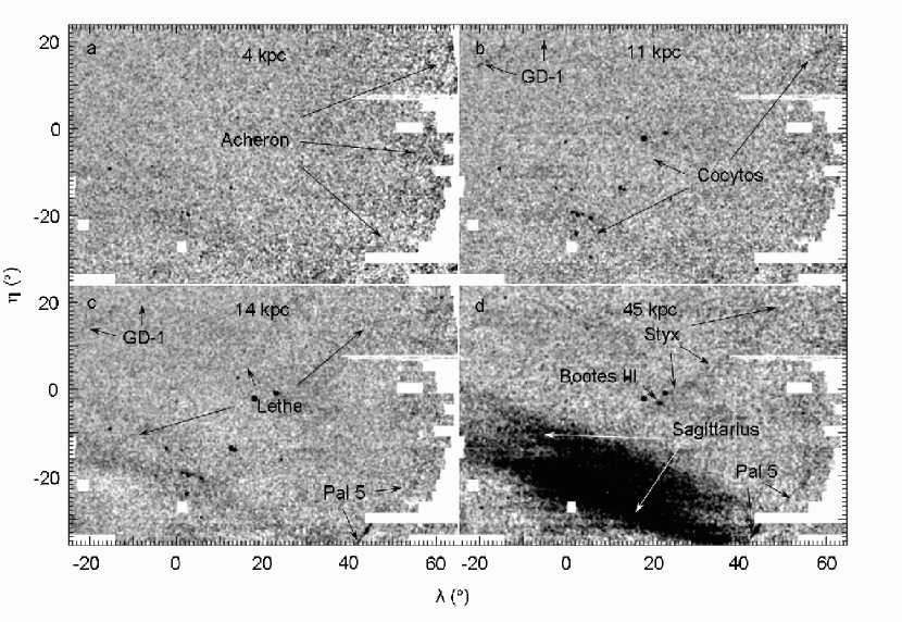
Figure 2.— Matched-filtered surface density maps of stars in the eastern 2/3rds of the DR5 Sloan Digital Sky Survey field. The stretch is logarithmic, and darker areas indicate higher surface densities. For panel (a) a 5th-order polynomial fit has been subtracted from the surface densities for presentation purposes. For the other three panels a 7th-order polynomial surface fit has been has been subtracted. All fields have been smoothed with a Gaussian kernel of width 0.2° . The white areas designate areas of missing data. Panels (a) through (d) result from shifting the M13 or M 15-matched filters by -1.4, +0.8, +1.1, and +3.2 magnitudes, respectively, and the corresponding distances (assuming $d_{M13}=7.7$ kpc and $d_{M15}=10.3$ kpc) are indicated.

The filtered surface density maps are the sum of maps generated using $g-r$ and $g-i$ filters as these colors best measure the turn-off and main sequence stars of interest. To improve the visibility of the streams in Figure 2, each image has been background subtracted by first masking out globular clusters and dwarf galaxies and then fitting a 5th or 7th order polynomial surface. These surface fits are shown in Figure 3. For the nearest of the streams, a 5th order polynomial fit is found to be sufficient to remove the rise in the number of disk stars at low Galactic latitudes. For the remaining streams a 7th order polynomial was used to subdue the increasing contribution from the Sagittarius stream. As is evident in Figure 3, there are no high-frequency features in the surface fits that could could be held to account for the streams visible in Figure 2. We emphasize that these background subtractions are purely for the purposes of presentation and we make no further use of them in our subsequent analysis.

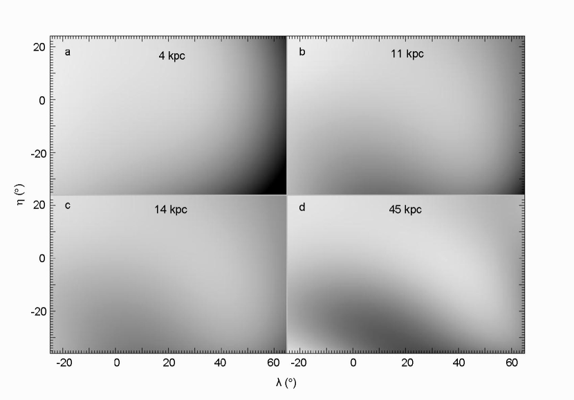
Figure 3.— Polynomial surface fits used to remove the background in Figure 2. Panel (a) is the result of using a 5-th order polynomial fit, while all other panels employ a 7th-order polynomial to reduce the effect of the Sagittarius stream. None of the streams in Figure 2 can be associated with the much lower frequency undulations visible here.

We compared Figure 2 with the reddening map of Schlegel, Finkbeiner, & Davis (1998) to ensure that apparent stellar over-densities are not due to localized changes in extinction. The reddening map covering the field of interest is shown in Figure 4. There is no apparent correlation between the new streams and the applied reddening corrections. The maximum values of $E(B-V)$ in the regions subtended by the new streams are $\sim 0.13$, with typical values of $<0.05$. Rerunning the matched filter analysis without reddening corrections has no significant effect on the location or the apparent strengths of the new features.

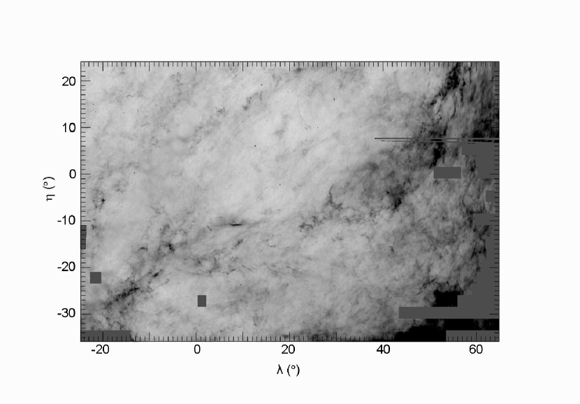
Figure 4.— $E(B-V)$ over the region of sky shown in Figure 2, as determined from the the DIRBE/IRAS dust maps of Schlegel, Finkbeiner, & Davis (1998). The stretch is linear, with darker regions corresponding to higher reddening. The reddening varies from $<0.05$ mag to 0.13 mag at the locations of the four streams.

We have also compared Figure 2 with similar maps made using the SDSS DR5 galaxy database to ascertain the extent to which confusion between stars and galaxies at faint magnitudes could contribute to the features we see. In none of the four cases presented here is there any indication of similar extended features in the distribution of galaxies.

3. Discussion

Visible in Figure 2 are several well known tidal features, as well as four new stellar debris streams. The new streams are much less pronounced than the Sagittarius, Pal 5, or GD-1 streams, and have average surface densities of between 5 and 50 stars deg^-2 The streams were initially detected and are most easily distinguished by viewing a rapid sequence of filtered images in which the filter is successively shifted to fainter and fainter magnitudes. The streams become apparent to the eye as linear features which often move from one side of the survey area to the other as one moves outward in distance.

All of the new streams span multiple constellations and none can be securely identified with a known progenitor at this time. For convenience, we extend traditional nomenclature and name the new streams after four mythical rivers in Hades: the Acheron (river of sorrow), Cocytos (lamentation), Lethe (forgetfulness), and Styx (hate).

3.1. Acheron

Visible in panel (a) of Figure 2 is a fairly narrow stream of stars extending some $37\arcdeg~{}$ across the southeastern corner of the DR5 survey area. The stream extends from the southern edge of Serpens Caput [($\lambda,\eta$) = (45°, -36°), (R.A., dec.) = (230°, -2°)] to the center of Hercules [($\lambda,\eta$) = (63°, 22°), (R.A., dec.) = (259°, 21°)], and is truncated at both the southern and eastern ends by the limits of the available data.

The stream is much less pronounced than (for example) GD-1 (Grillmair & Dionatos, 2006b) and in places the signal-to-noise ratio is almost vanishingly small. To better quantify the significance of the detection, we apply the following test: (i) We trace along the length of the putative stream, connecting the high points in the surface density distribution with segments that match the general curvature of the stream (though in this case there is almost none). (ii) We create a mask image of this trace, setting pixels along the trace and laterally out to 0.25°  in each direction to unity. All other mask pixels are set to zero. This width is chosen to roughly match the apparent width of the stream. (iii) We break the mask into seven stream segments, each approximately 5°  in length. (iv) For each stream segment, we successively shift the mask in the $\lambda$ direction across a representative portion of the sky, 0.1°  at a time, and multiply the mask by the filtered image in Figure 2. (v) For each segment, we fit a one dimensional, 3rd order polynomial to the mean filtered star counts as a function of lateral distance from the stream and subtract it. We exclude from this fit the region within 0.5°  of the stream. (vi) For each lateral offset, we compute the median of the background-subtracted responses over all segments. This last calculation serves as a continuity constraint and prevents strong biasing due to (for example) a single populous star cluster in in any one segment.

More succinctly, if we define $f(i,j)$ as the filtered star counts in a pixel with indices $i$ and $j$, and $m(i,j)$ as the stream-tracing mask, then the signal $s$ for stream segment $k$, shifted laterally by offset $d$, is:

$$s(d,k)=\frac{\sum_{i,j}[f(i,j)\times m(i+d,j)]}{n(d,k)},$$ (1)

where the summation is over all valid pixels (i.e. excluding portions of the Survey footprint with missing data). The total stream signal at offset $d$ is then:

$$T(d)={\rm median}[s(d,k)]_{k=1,...l},$$ (2)

where $l$ is the number of stream segments.

We plot the run of $T$ versus lateral offset for Acheron in Figure 5. The signal due to the stream is clearly visible as a broad peak approximately centered on a lateral offset of 0°. We note that perfect centering is not expected; aside from measurement uncertainties in regions with very little signal, the lateral profiles of real tidal streams need not be symmetric, depending on such factors as our line of sight to the stream and what portion of the stream’s orbit is being observed. If we regard $T$ beyond 1°  from the stream as being due to random clumping of stars and therefore a reasonable measure of the noise, we find $\sigma_{T}\approx 5$, where the standard deviation is measured after binning over the 0.5°  width of the mask. Integrating over the region $-1\arcdeg<d<1\arcdeg$ we find that we have detected the stream at the $\sim 10\sigma$ level. For comparison, a similar test applied to GD-1 yields a signal-to-noise ratio of $\sim 13$.

Figure 5.— Stream signal $T$ (described in the text) as a function of $\lambda$ offset from the Acheron stream. The dashed line shows the results of a similar test using an artificial stream with a Gaussian cross section and FWHM = 0.9°.

Also shown in Figure 5 is an identical test applied to an artificial tidal stream at the same location as Acheron and with a Gaussian cross section. The Gaussian which yields the best match to the observed stream profile has a full width at half maximum (FWHM) of 0.9°. While the physical cross section of the stream need not be Gaussian, the convolved artificial stream profile matches the actual stream profile reasonably well, and we use the best fitting FWHM as a convenient measure of the stream’s breadth. At a distance of 3.6 kpc (see below), this corresponds to a physical width of 60 pc. This is similar to the widths measured for the tidal tails of the globular clusters Pal 5 and NGC 5466 (Grillmair & Dionatos, 2006a; Belokurov et al., 2006a; Grillmair & Johnson, 2006) and the presumed cluster remnant GD-1 (Grillmair & Dionatos, 2006b). On the other hand, the width is much narrower than the tidal arms of the Sagittarius dwarf (Majewski et al., 2003; Martinez-Delgado et al., 2004) or the presumed dwarf galaxy streams discussed by Grillmair (2006a), Belokurov et al. (2006b), Belokurov et al. (2007), and Grillmair (2006b). This is consistent with the hypothesis that the stars making up the stream have very low random velocities, and that they were weakly stripped from a relatively small potential. Combining this with an orbit which passes low over the Galactic bulge (see below) suggests that the parent body is (or was) a globular cluster.

Following Grillmair & Dionatos (2006b) we shift the main sequence of the M 13-based filter brightward and faintward to estimate the stream’s distance. To avoid potential problems related to a difference in age between M 13 and the stream stars, we use only the portion of the filter with $19.5<g<22.5$, where the bright cutoff is 0.8 mags below M 13’s main sequence turn-off. This significantly reduces the contrast between the stream and the background (since turn-off stars contribute a substantial portion of the signal) but still provides sufficient signal to enable a reasonably precise measurement of peak contrast. We find that the strength of the southern end of the stream peaks at a magnitude shift of -1.53 mags, the central portion has the highest contrast at -1.58 mags, and the northernmost portion of the stream peaks at -1.73 mags. Adopting a distance to M 13 of 7.7 kpc (Harris, 1996), this puts the southern end of the stream at a heliocentric distance of 3.8 kpc, while the northern end is at 3.5 kpc. While the match between the color-magnitude distributions of stars in M 13 and in the stream is uncertain, the relative line-of-sight distances along the stream should be fairly robust; we estimate our random measurement uncertainties to be $\approx 10\%$.

Absolute distance estimates using this method depend not only on the uncertainty in the distance to M 13 but also on the CMD of foreground stars and the degree to which the metallicity (and hence color) of M 13’s main sequence matches that of the stream. We have only a very coarse estimate of the latter, namely the maximum contrast obtained for the stream when the star counts are processed with matched filters made from different globular clusters. If as a rough estimate of this uncertainty we take half the $g$ magnitude offset (0.46 mag) at a fixed color between the (dereddened) main sequence loci of M13 and M 15 (with [Fe/H] of -1.54 and -2.25, respectively), and combine this with a 5% uncertainty in the distance to M 13 (Grundahl et al., 1998), we arrive at a probable lower bound on the systematic distance uncertainty of 11%.

Integrating the locally background subtracted, filtered star counts over a width of $\approx 1\arcdeg~{}$ we find the total number of stars in the discernible stream to be $1300\pm 200$. For stars with $g<22.5$ the average surface density is $50\pm 5$ stars deg^-2, with occasional peaks of over 100 stars deg^-2. While these surface densities are similar to those found by Grillmair & Dionatos (2006b) for GD-1, Acheron appears considerably less pronounced. This is simply a consequence of the much larger number of contaminating foreground stars near the Galactic plane.

3.2. Cocytos

Visible in panel (b) of Figure 2 is a faint, narrow stream extending from Virgo [($\lambda,\eta$) = (1°, -35°), (R.A., dec.) = (186°, -3°)] in the south to Hercules [($\lambda,\eta$) = (65°, 20°), (R.A., dec.) = (259°, 20°)] in the east. The 80°   length of the stream is again limited by the extent of the SDSS survey area.

In Figure 6 we show the run of $T$ with lateral distance from the stream. In this case we have shifted our stream mask at a 45°  angle across Figure 2 and divided the stream mask into 12, $\sim 5\arcdeg$-long segments. We find that $\sigma_{T}\approx 5.0$ at $|d|>1\arcdeg~{}$ and, integrating from $-1\arcdeg<d<1\arcdeg$, determine that we have detected the stream at the $\sim 8\sigma$ level. Generating an artificial stream and applying the same test, we find that we obtain the best match to the observed profile using a Gaussian with FWHM = 0.7° . At a distance of 11 kpc (see below) this corresponds to a physical width of 140 pc. This is again similar to known globular cluster streams and argues that the progenitor of Cocytos is (or was) a globular cluster.

Figure 6.— As in Figure 5, but for the Cocytos stream. The artificial stream that best matches the observed $T$ profile has a Gaussian profile with FWHM = 0.7°.

The strength of both the southern and eastern ends of the stream peak at an M 13 main sequence magnitude shift of 0.9 mags. The estimated distance to the stream is therefore $11\pm 2$ kpc. Integrating the background subtracted, weighted star counts over a width of $\approx 1\arcdeg~{}$ we find the total number of stars in the discernible stream to be $500\pm 100$. For stars with $g<22.5$ the average surface density is between 5 and 8 stars deg^-2.

3.3. Lethe

Panel (c) of Figure 2 shows a faint stream extending from Hercules [($\lambda,\eta$) = (64°, 19°), (R.A., dec.) = (258°, 20°)] to Leo [($\lambda,\eta$) = (-13°, -14°), (R.A., dec.) = (171°, 18°)]. The stream extends from the eastern limit of the survey and appears to fade substantially in Leo, where it crosses the Sagittarius stream. There may be a continuation of the stream south of the Sagittarius stream but we have been unable to identify it with any confidence.

The apparent strength of Lethe relative to the distribution of foreground stars peaks at an M 13-relative offset of 1.3 mags at the eastern end, and about 1.0 mag at the western end. This puts the stream at a distance of between 12.2 and 13.4 kpc. Figure 7 shows the run of $T(d)$ for the stream, where again we have translated the stream mask at a 45°  angle across the filtered imaged in Figure 2 and subdivided the mask into 12 stream segments. In this case we find $\sigma_{T}=1.8$ at $|d|>1\arcdeg~{}$, and integrating within this region we find that Lethe is detected at the $7\sigma$ level. The best matching Gaussian stream shown in Figure 7 has a FWHM of 0.4°, which at 13 kpc corresponds to a physical width of 95 pc. Once again we conclude that Lethe is the debris stream of a globular cluster.

Figure 7.— As in Figure 5, but for the Lethe stream. The artificial stream that best matches the observed $T$ profile has a Gaussian profile with FWHM = 0.4°.

Integrating the background subtracted, weighted star counts over a width of $\approx 1\arcdeg~{}$ we find the total number of stars in the discernible stream to be $1100\pm 300$. For stars with $g<22.5$ the average surface density is 12 stars deg^-2, with the more pronounced regions of the stream having $\sim 30$ stars deg^-2.

3.4. Styx

Visible in panel (d) of Figure 2 is a broad stream extending west from Hercules [($\lambda,\eta$) = (63°, 21°), (R.A., dec.) = (259°, +21°)] to where it is overwhelmed by the much more populous Sagittarius stream in Coma Berenices [($\lambda,\eta$) = (8°, -12°), (R.A., dec.) = (194°, +20°)]. The contrast for Styx is improved if, instead of using a matched filter based on M 13, we use the SDSS CMD of M 15. This suggests that the CMD of stars in Styx is bluer than that of M 13. At the distance of Styx the stellar main sequence is almost entirely beyond the SDSS limiting magnitude. Consequently the main sequence fitting technique for estimating distance is not usable and we are forced to rely on turn-off and subgiant stars. Using the M 15 filter, the apparent contrast of the stream peaks at magnitude offsets of +2.8 mag at the western end, +3.2 mag in the central portion, and +3.4 at the eastern end. Adopting a distance to M 15 of 10.3 kpc (Harris, 1996), this translates to estimated distances of 38, 45, and 50 kpc, respectively. Owing to both the lack of a direct main sequence comparison and to the rather distended nature of the stream (which makes foreground estimation problematic), we regard these distances as very approximate until such time as deeper photometry becomes available.

Figure 8 shows the run of $T$ with lateral offset. For Styx we have used a mask width of 1°, divided the mask into 12, $\sim 4\arcdeg$-long segments, and shifted the mask solely in the $\eta$ direction. In this case we find $\sigma_{T}=0.18$ at $|d|>3\arcdeg~{}$, and integrating from -3°  to +3°  we find that Styx is detected at the $\sim 13\sigma$ level. The stream profile is noticeably asymmetric, with a fairly sharp northern edge but an excess of stars extending some 4°  to the south. This is qualitatively similar to the morphologies of tidal tails in N-body simulations (e.g. Choi, Weinberg, & Katz (2007)). The artificial stream which best matches the primary component of Styx has a FWHM of 3.3°. At a distance of 45 kpc this corresponds to 2.6 kpc. This is much broader than the presumed globular cluster streams above, but is similar to the the dwarf galaxy streams discussed by Grillmair (2006a), Belokurov et al. (2007), and Grillmair (2006b), though narrower by half compared to the Sagittarius stream (Majewski et al., 2003; Martinez-Delgado et al., 2004; Belokurov et al., 2006b). We conclude that this stream is most likely debris from a dwarf galaxy.

Figure 8.— As in Figure 5, but for the Styx stream. The artificial stream that best matches the observed $T$ profile over the region $-3\arcdeg<d<3\arcdeg$ has a Gaussian profile with FWHM = 3.3°. The stream is clearly asymmetric, with an extended spray of stars to the south, and a fairly sharp cut off on the northern side.

3.5. Bootes III: A New Dwarf Galaxy?

With a contrast maximum at very nearly the same distance ($\sim 46$ kpc) as the Styx stream is a relatively compact feature at [($\lambda,\eta$) = (21.6°, -3.5°), (R.A., dec) =(209.3°, 26.8°)]. The object has a filtered star count surface density many times higher than any visible portion of Styx and is clearly distinct within the stream. Panel (a) of Figure 9 shows the filtered star count distribution in the immediate vicinity of this object. Galaxy cluster ACO 1824 lies within 3′  of the location of this object(Abell, Corwin, & Olowin, 1989); could the apparent over-density be due to SDSS misclassification of stars at faint magnitudes? In panel (b) of Figure 9 we show the distribution of objects classified as galaxies in DR5, where we have used a filter identical to that used in panel (a). There is little correspondence between the two distributions, and certainly no concentration of objects at the same position. We conclude that this over-density is due to an equidistant collection of stars orbiting in the outskirts of our own Galaxy and we henceforth designate it Bootes III.

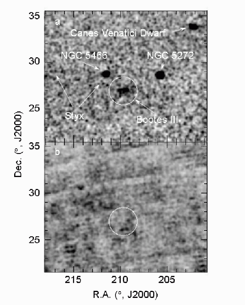
Figure 9.— (a) Matched-filtered surface density map in the immediate vicinity of Bootes III, smoothed with a Gaussian kernel of width 0.1°, at an M 15-relative magnitude shift of 3.2 mags. Darker areas indicate higher surface densities and the stretch is linear. Though at very different distances, NGC 5466, NGC 5272, and the Canes Venatici dwarf (Zucker et al., 2006) are also visible by virtue of their high surface densities and the overlap of parts of their CMDs with the M 15 filter. (b) The distribution of objects classified as galaxies in DR5, where we have used a filter identical to that used in panel (a).

Figure 10 shows a contour plot of the filtered star counts in and around Bootes III; the object appears somewhat double-lobed, possibly disturbed, and extends $\approx 1.5\arcdeg~{}$ from east to west. At 46 kpc this corresponds to a spatial extent of about $\sim 1$ kpc. If the stellar populations in the eastern and western lobes of Bootes III are identical, then the difference in the filter shifts required to maximize the apparent contrast indicates that the eastern lobe of the galaxy is some 3 kpc closer to us than the western lobe. If the two lobes are indeed part of the same structure then Bootes III must be highly elongated along the line of sight. Figure 11 shows a surface density profile of Bootes III, where we have counted all stars with $g<22.7$ and $-1<g-i<1$. The galaxy is evidently quite extended, with a power-law surface density profile that goes as $\sigma\propto r^{-1.0\pm 0.2}$. Integrating the background-subtracted counts out to 1°  we find a total of 302 stars with $g\leq 22.7$ which we can reasonably attribute to Bootes III.

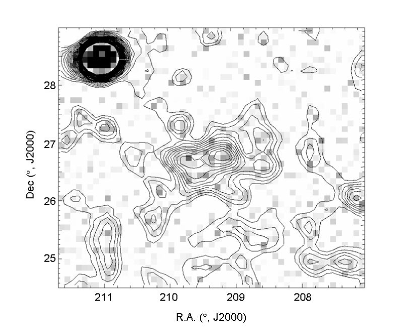
Figure 10.— Contour plot of a region centered on Bootes III. The underlying image has been smoothed with a Gaussian kernel of 6′. Contours are spaced linearly, and the strong source to the northeast of Bootes III is NGC 5466.

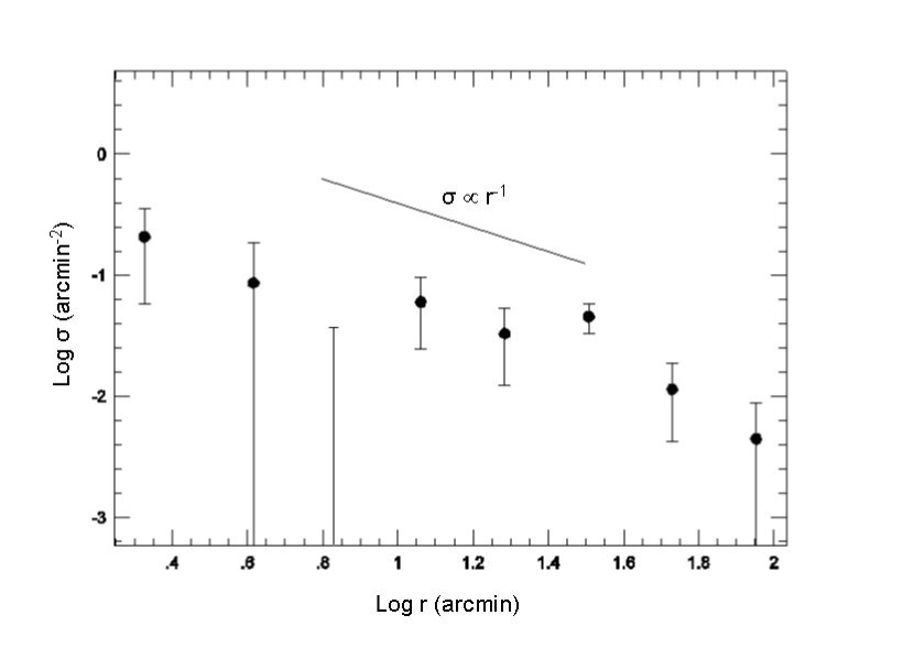
Figure 11.— The (unfiltered) surface density profile of all stars with $g<22.7$ and $-1<g-i<1$. The center of Bootes III is taken to be at (R.A., dec) = (209.281°, 26.775°). The surface densities have been background subtracted using the measured counts in an annulus extending from 1.5°  to 2°.

As is the case for Styx, using the SDSS color-magnitude distribution of stars in M 15 as the basis for the matched filter yields a slightly higher contrast between the galaxy and the foreground population. The inference is that the age and/or metallicity of Bootes III and the stream are more similar to that of M 15 than M 13. At 46 kpc the galaxy is revealed almost entirely by subgiant and turn-off stars; removing the red giant branch from the filter has little effect on the apparent contrast. Figure 12 shows the color-magnitude distribution of all stars within 1°  of the center of Bootes III. Here we have subtracted the distribution of stars in several regions around Bootes III over an area of $\sim 60$ square degrees. Comparing with the CM loci of M 13 and M 15 (shifted vertically to a distance of 46 kpc), there is a clear overdensity of stars along the expected positions of the main sequence turn-off, the subgiant branch, and the lower giant branch. Consistent with the filter responses above, the CM locus of M 13 is evidently $\sim 0.1$ mag too red to match the apparent distribution. The M 15 locus clearly provides a better match to the data.

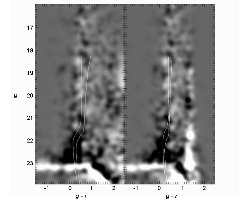
Figure 12.— The background-subtracted, color-magnitude distribution of all stars lying within 1°  of the center of Bootes III. Darker areas indicate enhancements over the background distribution. Stars were binned in color and magnitude and smoothed with a Gaussian kernel of $\sigma=0.1$. The distribution was background-subtracted using similarly binned and smoothed color-magnitude distributions in regions spaced around Bootes III and the two nearby globular clusters and covering a total of $\sim 60$ square degrees. Also shown are the $g,g-i$ and $g,g-r$ color-magnitude loci for M 13 (to the red) and M 15 (to the blue), as derived from SDSS photometry.

In Figure 13 we show the CMD of all stars within 0.8°  of the center of Bootes III. While the turn-off, subgiant, and red giant branches of Bootes III are lost among the unsubtracted foreground stars in this figure, there is a clear concentration of stars at the expected location of the blue horizontal branch (BHB). Fitting the BHB sequence tabulated for the SDSS system by Sirko et al. (2004), we find $(M-m)_{0}=18.35\pm 0.01$. Corresponding to a distance of 46.7 kpc, this is in excellent agreement with our maximum contrast distance estimate above. In Figure 14 we show the distribution of stars selected to have colors and magnitudes consistent with Bootes III’s BHB. There is an apparent enhancement of such stars across the face of Bootes III, though just as for the turn-off stars sampled using the matched filter, the distribution of BHB stars is not very centrally concentrated. The BHB star distribution is considerably more extended in the east-west direction (much like the filtered star counts in Figures 9 and 10), subtending nearly 2°on the sky.

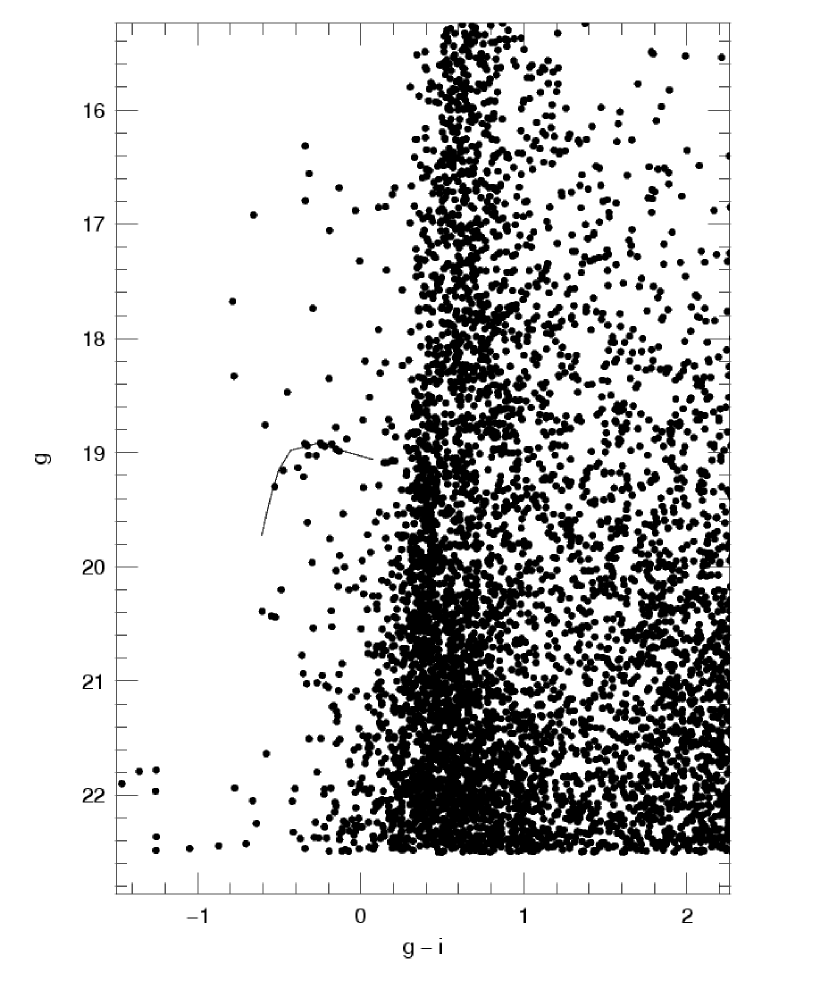
Figure 13.— The color-magnitude distribution of stars within 0.8°  of the center of Bootes III. A blue horizontal branch is clearly visible at $(g,g-i)\approx 19,-0.25$). The solid line shows the predicted SDSS blue horizontal branch sequence of Sirko et al. (2004), shifted vertically by 18.35 mags.

Figure 14.— The sky distribution of candidate Bootes III blue horizontal branch stars. Based on the CMD in Figure 13, the stars are selected to have $18.7<g<19.3$ and $-0.55<g-i<-0.07$.

All the evidence is consistent with Bootes III being a dwarf galaxy (or a remnant thereof). Combined with its apparent location at the same distance as Styx and very nearly in the middle of it, we infer that Bootes III is both physically associated with the stream and quite possibly its progenitor. Its broad spatial extent, its low surface density and power-law profile, its possibly disturbed morphology, and its location within Styx, all suggest that Bootes III may be in or nearing the final throes of tidal dissolution.

4. Constraints on Orbits

Though a lack of velocity information prevents us from tightly constraining the orbits of the streams, the apparent orientations of the streams combined with our distance estimates can yield some initial constraints. We use the Galactic model of Allen & Santillan (1991), which assumes a spherical halo potential. We employ a least squares method to fit both the stream orientations on the sky and our estimated distances. The tangential velocities at each point are primarily constrained by the projected paths of the streams while our relative distance estimates help to limit the range of possible radial velocities at any point.

We fit to a number of normal points lying along the estimated centerlines of each stream. We adopt a solar Galactocentric distance of 8.5 kpc, and distance uncertainties of 1.0, 2.5, 2.5, and 10 kpc for Acheron, Cocytos, Lethe, and Styx, respectively. We choose fiducial points in each stream for radial velocity predictions based in part on the apparent strength of the stream at those locations. When selecting targets for follow-up spectroscopy, these regions will presumably have the largest concentrations of stream stars and thus the highest targeting priority. The predicted heliocentric radial velocities and proper motions at the fiducial points are listed in Table 1. The uncertainties correspond to the 90% confidence interval for each parameter and do not take account of inaccuracies in the model potential. Predictions are provided for both prograde and retrograde orbits. Three-view projections of the best fit orbits are shown in Figure 15.

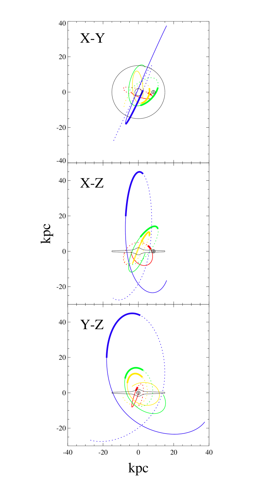
Figure 15.— Orbit projections for the four new streams in X, Y, Z Galactic coordinates. The red curve corresponds to Acheron, yellow to Cocytos, green to Lethe, and Styx is represented by the blue curve. The heavy lines show the portions of the orbits visible in Figure 1. The thin solid curves show the orbits integrated forward in time while the dotted portions of the curves show the same orbit integrated backwards. The Sun’s position at (X,Y,Z) = (8.5,0,0) kpc is indicated.

Do the computed orbits suggest possible associations between the new streams and known residents of the halo? Integrating orbits for a sufficiently long time, one is almost certain to pass near the current positions of known globular clusters. However, given our limited knowledge of the Galactic potential and the rather rudimentary orbit constraints determined above, such an exercise would clearly be pointless. However, if we limit ourselves to integrating orbits no more than once around the Galaxy, we can match the computed positions, distances, and radial velocities against the 150 globular clusters compiled by Harris (1996). Setting rejection limits of 5°  in sky position, 5 kpc or a 30% difference in distance, and 50 km s^-1 in radial velocity, we can say that there are no known globular clusters that match our orbits simultaneously in position, distance, and radial velocity. Similarly, other than Bootes III there are no known dwarf galaxies that lie along the integrated orbit of Styx. While the uncertainties in our orbit estimates do not allow us to make strong statements at this point, our results are consistent with the hypothesis that the newly detected globular cluster streams are remnants of clusters that have long since been whittled away to nothing.

5. Conclusions

Applying optimal contrast filtering techniques to SDSS data, we have detected four new stellar streams in the Galactic halo, along with a probable dwarf galaxy in possibly the final throes of tidal disruption. Three of the streams are spatially very narrow and are likely to be the remnants of extant or disrupted globular clusters. The fourth stream is much broader, similar in width to the Orphan and Anticenter streams, and presumably constitutes the tidal debris of a dwarf galaxy. Bootes III, the new dwarf galaxy candidate, appears to lie near the middle of this stream and may well be its progenitor. Based on an apparently good match to the color-magnitude distribution of stars in M 13 and M 15, we conclude that the stars making up the streams are old and metal poor, with the Styx stream and Bootes III being the oldest and/or most metal poor.

A determination of the nature and the properties of our dwarf galaxy candidate with deep imaging are the subject of a forthcoming paper (Grillmair, Hamam, & Laher, 2008, in preparation). If indeed Bootes III is in the final throes of tidal dissolution, it will be a particularly interesting target for detailed kinematic studies. Refinement of the stream orbits will require radial velocity measurements of individual stars, though given the very low stellar surface densities in these streams, this will necessarily be an ongoing task. In this respect, these streams may be particularly well suited for upcoming spectroscopic survey instruments such as LAMOST.

Table 1Predicted Motions and Orbit Parameters

Stream	Fiducial Point		Prograde Orbit			Retrograde Orbit
	R.A.	dec	$v_{r}$	$\mu_{\alpha}$ cos($\delta$)	$\mu_{\delta}$	$v_{r}$	$\mu_{\alpha}$ cos($\delta$)	$\mu_{\delta}$	$R_{peri}$	$R_{apo}$
	J2000		km s-1	mas yr-1	mas yr-1	km s-1	mas yr-1	mas yr-1	kpc	kpc
Acheron	15 50 24	+9 48 39	$-240^{+99}_{-78}$	$-3.5\pm 0.5$	$-4.2\pm 0.3$	$136^{+104}_{-74}$	$-12.5\pm 0.5$	$-13.3\pm 0.3$	$3.5\pm 0.8$	$9.2\pm 3.3$
Cocytos	16 29 21	+26 40 8	$-142\pm 10$	$0.51\pm 0.07$	$-3.80\pm 0.05$	$-92\pm 10$	$-5.8\pm 0.1$	$-1.0\pm 0.05$	$4.9\pm 0.2$	$12.5\pm 0.2$
Lethe	16 15 45	+29 56 45	$-134\pm 13$	$+0.67\pm 0.19$	$-3.46\pm 0.04$	$-105\pm 13$	$-5.1\pm 0.2$	$-0.40\pm 0.03$	$7.7\pm 0.4$	$17.3\pm 0.5$
Styx	13 56 24	+26 48 00	$-42^{+44}_{-191}$	$-0.23^{+0.09}_{-0.17}$	$-0.6\pm 0.03$	$-22^{+182}_{-44}$	$-1.05\pm 0.09$	$-0.95\pm 0.03$	$13.7\pm 3.9$	$45^{+38}_{-1}$

References

- Abell, Corwin, & Olowin (1989) Abell, G. O., Corwin, H. G. Jr., & Olowin, R. P. 1989, ApJS, 70, 1
- Allen & Santillan (1991) Allen, C., & Santillan, A. 1991, Rev. Mex. Astron. Astrofis., 22, 255
- Belokurov et al. (2006a) Belokurov, V., Evans, N. W., Irwin, M. J., Hewett, P. C., & Wilkinson, M. I. 2006a, ApJ, 637, 29
- Belokurov et al. (2006b) Belokurov, V., et al. 2006b, ApJ, 642, 137
- Belokurov et al. (2007) Belokurov, V., et al. 2007, ApJ, 658, 337
- Choi, Weinberg, & Katz (2007) Choi, J.-H., Weinberg, M. D., & Katz, N. 2007, MNRAS, 381, 987
- Combes, Leon, & Meylan (1999) Combes, F., Leon, S., & Meylan, G. 1999, A&A, 352, 149
- de Marchi (1999) de Marchi, G. 1999, AJ, 117, 303
- Gnedin & Ostriker (1997) Gnedin, O. Y., & Ostriker, J. P. 1997, ApJ, 474, 223
- Grillmair (2006a) Grillmair, C. J. 2006a, ApJ, 645, 37
- Grillmair (2006b) Grillmair, C. J. 2006b, ApJ, 651, 29
- Grillmair & Johnson (2006) Grillmair, C. J., & Johnson, R. 2006, ApJ, 639, 17
- Grillmair & Dionatos (2006a) Grillmair, C. J., & Dionatos, O. 2006a, ApJ, 641, 37
- Grillmair & Dionatos (2006b) Grillmair, C. J., & Dionatos, O. 2006b, ApJ, 643, 17
- Grillmair, Hamam, & Laher (2008, in preparation) Grillmair, C. J., Hamam, N., & Laher, R. 2008, in preparation.
- Grundahl et al. (1998) Grundahl, F., Vandenberg, D. A., & Anderson, M. I. 1998, ApJ, 500, 179
- Harris (1996) Harris, W. E. 1996, AJ, 112, 1487
- Jordi, Grebel, & Ammon (2006) Jordi, K., Grebel, E. K., & Ammon, K. 2006, å, 460, 339
- Koch et al. (2004) Koch, A., Grebel, E. K., Odenkirchen, M., Martinez-Delgado, D., & Caldwell, J. A. R. 2004, AJ, 128, 2274
- Martinez-Delgado et al. (2004) Martinez-Delgado, D., Gomez-Flechoso, M., Aparicio, A., & Carrera, R. 2004, ApJ, 601, 242
- Majewski et al. (2003) Majewski, S. R., Skrutskie, M. F., Weinberg, M. D., & Ostheimer, J. C. 2003, ApJ, 599, 1082
- Murali & Dubinski (1999) Murali, C., & Dubinski, J. 1999, AJ, 118, 911
- Odenkirchen et al. (2001) Odenkirchen, M., et al. 2001, ApJ, 548, 1650
- Odenkirchen et al. (2003) Odenkirchen, M. et al. 2003, AJ, 126, 2385
- Rocha-Pinto et al. (2004) Rocha-Pinto, H. J., Majewski, S. R., Skrutskie, M. F., Crane, J. D., Patterson, R. J. 2004, ApJ, 615, 732
- Rockosi et al. (2002) Rockosi, C. M. et al. 2002, AJ, 124, 349
- Schlegel, Finkbeiner, & Davis (1998) Schlegel, D. J., Finkbeiner, D. P., & Davis, M. 1998, ApJ, 500, 525
- Sirko et al. (2004) Sirko, E., Goodman, J., Knapp, G. R., Brinkman, J., Ivezic, Z., Knerr, E. J., Schlegel, D., Schneider, D. P., & York, D. G. 2004, AJ, 127, 899
- Yanny et al. (2003) Yanny, B. et al. 2003, ApJ, 588, 824
- Zucker et al. (2006) Zucker, D. B. et al. 2006, ApJ, 643, L103