Conductance of a single-atom carbon chain with graphene leads

Abstract

We study the conductance of an interconnect between two graphene leads formed by a single-atom carbon chain. Its dependence on the chemical potential and the number of atoms in the chain is qualitatively different from that in the case of normal metal leads. Electron transport proceeds via narrow resonant states in the wire. The latter arise due to strong reflection at the junctions between the chain and the leads, which is caused by the small density of states in the leads at low energy. The energy dependence of the transmission coefficient near resonance is asymmetric and acquires a universal form at small energies. We find that in the case of leads with the zigzag edges the dispersion of the edge states has a significant effect on the device conductance.

I Introduction

The efforts to miniaturize electronic devices have long motivated studies of electron transport in molecular and atomic scale devices. Creating reliable electrical contacts with the molecule presents a major challenge in molecular electronics. Until recently, in molecular electronic devices the molecule was typically attached between two normal metal, such as gold, electrodes Reed1997 ; Reed1999 ; Park2000 ; Park2002 ; Liang2002 ; AtomicContacts .

Carbon-based conductors have long been expected to be promising components of electronic devices McEuen1998 . Apart from bulk graphite there are also quasi-one dimensional (carbon nanotubes Iijima ) and two-dimensional (graphene graphene_Geim ) forms, which have remarkable mechanical and electrical properties and form strong chemical bonds with each other. This offers the prospect of building entire electronic devices or circuits out of carbon-based materials.

Single-atom carbon chains (SACCs) are natural components of such devices. They are expected to be ideal one-dimensional conductors Avouris . They covalently bond to other carbon materials. Formation of SACCs was conjectured to occur between carbon nanotubes Richter ; NanoLettersChains ; Louie and in gaps between two graphene leads Marc . Formation of SACCs between graphene electrodes fabricated by stretching a graphene strip has been observed in Ref. Jin2009, . SACC interconnects between graphene leads could form a basic unit for integration into more complicated circuits in the future. Electron transport through SACCs with graphene contacts has not been studied theoretically. We address this issue in the present paper.

Electron transport in SACCs with metal leads has been studied numerically Avouris ; Larade2001 ; Tongay2004 ; Crljen2007 . The conductance of an SACC strongly coupled to metal electrodes is of order of the conductance quantum and exhibits even-odd oscillations with the number of atoms in the chain, with the contrast ratio of order unity.

In this paper we show that electron transport through an SACC interconnect between graphene leads in the non-interacting electron approximation is described by an analytically solvable model. This enables us to gain physical insight into the essential features of electron transport. This model can also serve as the starting point for treating one-dimensional electron correlations in SACC and their influence on transport.

The conductance of the system is qualitatively different from that in the case of metal leads. For all electron energies corresponding to practically relevant temperatures and doping levels the junction between the chain and the graphene lead is almost perfectly reflecting even at strong coupling between the chain and the lead. The transmission coefficient of the contact vanishes linearly with electron energy as the latter approaches the Fermi energy of undoped graphene. This suppression of transmission results from the vanishing of density of states (DoS) in graphene at zero doping. As a result electron transport through the interconnect proceeds via narrow resonant states in the chain that arise due to strong reflection at the junctions. The width and the position of the resonances depend on the length of the interconnect and the details of its coupling to the leads. The shape of low energy resonances is universal but markedly different from the Breit-Wigner form. It is dictated by the linear energy dependence of the DoS in graphene at the point of contact with the chain. This holds even in the case of leads with zigzag edges, which support edge states edge_1996 ; prb1996 . Although edge states have a linear dispersion at low energies, their wave functions extend into the bulk to distances inversely proportional to the energy and give a linear in energy contribution to DoS at the contact point.

Due to the resonant character of transmission the device conductance is very sensitive to the number of atoms in the chain. In the case of graphene leads the conductance difference between chains with odd and even number of atoms in the SACC (which was first noted Avouris in the case of metal leads) becomes much more pronounced and appears as the difference between the on- and off- state conductance.

The high stability of SACC interconnects makes them promising building block of atomic scale electronics of the future. The resonant character of electron transport through them suggests that they can be used as components of atomic scale transistors. Our work is the first step towards theoretical understanding of electron transport in SACC interconnects between graphene leads.

The paper is organized as follows. In Sec. II we qualitatively discuss the essential features of electron transport in SACC interconnects between graphene leads. In Sec. III we formulate an analytically solvable model of electron dynamics in the system. In Sec. III.1 we derive a general formula for the reflection amplitude of the junction between the chain and the lead in terms of the electron Green function (GF) of the lead. In sec. III.2 we evaluate the GF and study the tunneling density of states at the junction due to the bulk and edge electron states in the lead. In sec. IV we evaluate the transmission coefficient of the device and obtain the universal formula for the resonance shape. We discuss our results and experimental implications in Sec. V.

II Qualitative discussion

Linear molecules with degenerate electron states represent an exception to the Jahn-Teller theorem on the instability of the symmetric molecular configurations Landau_QM . In this case the degenerate electron states have nonzero angular momenta $\pm\Lambda$ about the molecule axis. Thus the matrix element coupling the two states and the corresponding energy gain arises only in second or higher order in the vector displacements of the nuclei from the symmetry axis. In the linear SACC the two degenerate electron bands have angular momenta $\pm 1$ about the molecular axis, and their coupling arises only in second order in the nuclear displacements. In the Peierls channel, which at zero doping corresponds to dimerization, the coupling between right and left movers is linear in the displacements. Thus the two most likely candidates for the SACC structure are the linear chain of equidistant double bonded carbon atoms, known as cumulene ($\cdots\mathrm{C}=\mathrm{C}=\mathrm{C}=\mathrm{C}\cdots$), and the Peierls-distorted dimerized chain, known as polyyne ($\cdots\mathrm{C}-\mathrm{C}\equiv\mathrm{C}-\mathrm{C}\cdots$). This expectation is confirmed by numerical studies. Ab initio calculations Tongay2004 show that because of large quantum fluctuations of the atomic positions, among all possible spatial arrangements of the carbon atoms in the chain only the cumulene structure is stable. The outer shell electron orbitals in cumulene are $sp$-hybridized. The two $sp$ hybridized orbitals form the fully occupied $\sigma$ band. The two remaining $p_{y}$ and $p_{z}$ orbitals form two doubly degenerate $\pi$ bands, which are half filled making undoped cumulene a one-dimensional conductor. Numerical studies Okano2007 also show that cumulene remains metallic under doping.

If the SACC attached to the graphene leads is not too long the main features of electron transport through it can be understood within the single electron picture without accounting for electron-electron correlations.

As the conduction $\pi$ band in graphene leads is formed by the $p_{z}$ orbitals, which are perpendicular to the graphene plane, only the electrons from the $\pi_{z}$ band in SACC can propagate into the leads. Thus electron transport is mediated by a single conducting band in the chain.

Because of the long mean free path of electrons in graphene graphene_Geim , electron motion in the leads may be assumed to be ballistic. The device conductance is then determined by the elastic electron scattering at the junctions between the molecular wire and the leads and backscattering in the chain. Backscattering in the SACC due to electron-phonon interaction corresponds to emission or absorption of phonons with a wavelength of order of the interatomic spacing and energy of the order of $10^{3}K$. As a result such processes are exponentially suppressed Seelig1 ; Seelig2 even at room temperature. Although imperfections in the substrate and deviations of the atomic positions from the ideal configuration cause some backscattering of electrons in the wire, we show below that the strongest reflection of the electron wave in the chain occurs at the contact with the graphene lead.

With the aid of the Fermi golden rule the transmission coefficient of the contact can be estimated as $\mathcal{T}_{c}\sim|\gamma_{c}|^{2}\nu_{w}\nu_{g}$. Here $\gamma_{c}$ is the tunneling matrix element that couples the last atom in the chain to the lead, $\nu_{w}$ is the local DoS at that atom and $\nu_{g}$ the DoS an the graphene atom that is connected to the chain. The local DoS in the chain is energy independent and can be estimated as $\nu_{w}\sim 1/\gamma_{w}$, where $\gamma_{w}$ is the nearest neighbor hopping integral in the atomic wire. The DoS in graphene, on the other hand is strongly energy dependent and is of the order of $\nu_{g}\sim|\epsilon|/\gamma_{g}^{2}$, where $\gamma_{g}$ is the nearest neighbor hopping integral in graphene and $\epsilon$ is the electron energy measured from the Fermi level of undoped graphene . Thus the transmission coefficient of the contact can be estimated as

$$\mathcal{T}_{c}\sim\frac{\gamma^{2}_{c}|\epsilon|}{\gamma_{w}\gamma_{g}^{2}}.$$ (1)

The hopping integrals in graphene and SACC are of the same order of magnitude. Therefore at typical doping levels, $|\epsilon|\ll\gamma_{g}$, the transmission coefficient is small even at strong coupling between the chain and the lead, when all hopping integrals between nearest neighbor carbon atoms are of the same order, $\gamma_{c}\sim\gamma_{w}\sim\gamma_{g}$.

Neglecting the weak backscattering in the wire we can express the energy-dependent transmission coefficient of the device, $\mathcal{T}(\epsilon)$, in terms of the reflection amplitudes of the left and right junction between the wire and the leads, $r_{l/r}(\epsilon)=|r_{l/r}(\epsilon)|\exp(i\delta_{l/r})$, as

$$\mathcal{T}(\epsilon)={|t_{l}(\epsilon)|^{2}|t_{r}(\epsilon)|^{2}\over(1-|r_{l}(\epsilon)||r_{r}(\epsilon)|)^{2}+2|r_{l}(\epsilon)||r_{r}(\epsilon)|(1-\cos\phi)}.$$ (2)

Here $|t_{l/r}(\epsilon)|^{2}=1-|r_{l/r}(\epsilon)|^{2}$ are the transmission coefficients of the junctions, and $\phi$ is the phase accumulated by an electron upon returning to the same point in the chain after being reflected from both contacts. It can be expressed as $\phi=2k\mathcal{N}+\delta_{l}+\delta_{r}$, where $\mathcal{N}$ is the number of atoms in the chain, $k$ is the absolute value of the dimensionless (measured in units of the inverse lattice spacing $d$ of the chain) electron quasimomentum, and $\delta_{l/r}$ are the phases of the reflection amplitudes of the contacts.

Because at low energies the junctions become strongly reflective appreciable transmission through the device in this regime occurs only near resonances, where the phase $\phi$ equals an integer multiple of $2\pi$. The energy spacing between adjacent resonances is $\sim\gamma_{c}/\mathcal{N}$.

To obtain a simplified expression for the transmission coefficient near a low energy resonance we write the reflection amplitudes of the junctions at low energies as $|r_{l/r}(\epsilon)|=1-c_{l/r}|\epsilon|/\gamma_{g}$, where $c_{l/r}$ is a numerical coefficient of the order of unity. This expression follows from Eq. (1). Linearizing the energy dependence of the phase $\phi$ near the resonance energy $\epsilon_{0}$, $\phi=c_{\phi}(\epsilon-\epsilon_{0})/\gamma_{g}$, where $c_{\phi}\sim\mathcal{N}$ is a numerical coefficient, we can write the transmission coefficient of the device as,

$$\mathcal{T}(\epsilon)=\left[\mathcal{T}_{0}^{-1}+\alpha\left(1-\frac{\epsilon_{0}}{\epsilon}\right)^{2}\right]^{-1}.$$ (3)

Here $\mathcal{T}_{0}=(c_{l}+c_{r})^{2}/(4c_{l}c_{r})$ is the transmission coefficient at the resonance, and $\alpha=c_{\phi}^{2}/(4c_{l}c_{r})\sim\mathcal{N}^{2}$.

The width of the resonance is of the order of $\epsilon_{0}/\mathcal{N}$. In the case of symmetric contacts, $c_{l}=c_{r}$, the device becomes perfectly transmitting on resonance. The shape of the resonance is shown in Fig. 4. It is strongly asymmetric and markedly different from the Breit-Wigner form which arises in the case of metal leads.

Since low energy transmission through the device proceeds via a single resonant state in the chain it is clear that Eq. (3) holds under very general conditions. The assumption that the coupling $\gamma_{c}$ between the chain and the lead is energy independent is valid if the resonance energy is smaller than the inverse propagation time of an electron across the junction. Such resonances always exist if the SACC is longer than the junction (for example a small peninsular extending between the graphene lead and the chain). As long as the backscattering in the chain does not lead to localization the resonant state will remain coupled to both leads. The backscattering will merely modify its energy and strength of coupling to the leads, and can be accounted for by the change of parameters in Eq. (3). Similarly electron-electron interactions in a finite chain will renormalize the energy and the coupling of the resonant state with the leads.

In the remainder of the paper we present a quantitative treatment of simple model of electron transport through an cumulene SACC interconnect between graphene leads.

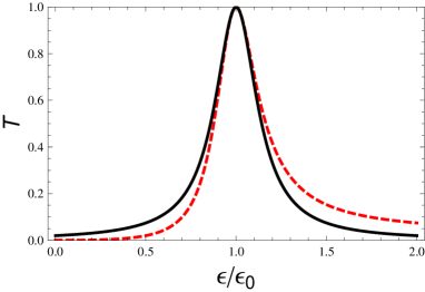
Figure 1: Color online. Dependence of the transmission coefficient $\mathcal{T}$ in Eq. (35) on $\epsilon/\epsilon_{0}$ (dashed line) with $N=10$ and $\alpha\sim 1$. The solid curve is the Breit-Wigner resonance with the same resonance energy $\epsilon_{0}$ and width.

III System and model

Consider an ideal cumulene SACC connected to graphene leads with perfect zigzag edges, as shown in Fig. 2

As a first step in the theoretical analysis of the system, we assume that the atoms in the SACC are in the ideal cumulene configuration. We work in the noninteracting electron approximation and describe the electron motion in the conducting $\pi_{y}$ and $\pi_{z}$ bands using the nearest neighbor tight binding approximation. More complicated band structure of the carbon wire will not significantly modify our conclusions.

Electron transport through the device is fully determined by the reflection amplitude of the contact between the SACC and the graphene lead. We derive in Sec. III.1 a general formula for the reflection amplitude of the contact in terms of the local DoS in the lead evaluated at the atom which is connected to the SACC, Eq. (14). This expression is applies for an arbitrary shape of the lead. Then in Sec. III.2 we specialize to the case of graphene leads with zigzag edge. The zigzag edge is likely to be formed as a result of an electric failure Marc or a tear of a graphene strip because it has the least number of dangling bonds per unit length. We find that the edge states present in the case of zigzag edge provide a significant contribution to the tunneling DoS at the edge of the lead, and thus carry a significant portion of the current through the device.

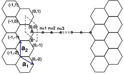
Figure 2: Schematic picture of the device. The atoms in the wire are labeled by $n=1,2,\ldots$. The unit vectors of the graphene Bravais lattice, $\mathbf{a}_{1}$ and $\mathbf{a}_{2}$, are shown by blue arrows. Each unit cell (dashed rhomboid) is labeled by $(N_{1},N_{2})$.

III.1 Reflection amplitude of the junction

Let us first consider a single junction between the SACC and a graphene lead. We label the sites in the chain by an integer $n$ which enumerates the atoms starting from the junction, see Fig. 2. The reflection amplitude of the contact can be found from the retarded Green function of the auxiliary system evaluated between two points inside the semi-infinite wire using the expression,

$$G(n,n^{\prime})\sim\exp[-ik|n-n^{\prime}|]+r(\epsilon)\exp[-ik(n+n^{\prime})].$$ (4)

Here $k$ is the absolute value of the energy-dependent quasimomentum of the electron in the chain, and the Green function is defined in terms of the system Hamiltonian $\hat{H}$ in the standard way,

$$G(n,n^{\prime})=\langle n|\hat{G}|n^{\prime}\rangle=\langle n|(\epsilon_{+}-\hat{H})^{-1}|n^{\prime}\rangle,$$ (5)

where $\epsilon_{+}=\epsilon+i0$.

We write Hamiltonian of the system as

$$\hat{H}=\hat{H}_{w}+\hat{H}_{g}+\hat{V},$$ (6)

where $\hat{H}_{w}$ and $\hat{H}_{g}$ are respectively the Hamiltonians of the semi-infinite wire and the semi-infinite graphene lead, and $\hat{V}$ is the perturbation, which describes electron tunneling between them.

Introducing the Green function of the unperturbed system , $\hat{G}_{0}=(\epsilon_{+}-\hat{H}_{w}-\hat{H}_{g})^{-1}$, we can express the Green function of the full system as

$$\hat{G}=\hat{G}_{0}+\hat{G}_{0}\hat{T}\hat{G}_{0},$$ (7)

where $\hat{T}$ is the $T$-matrix of the junction between the chain and the lead given by

$$\hat{T}=(1-\hat{V}\hat{G}_{0})^{-1}\hat{V}.$$ (8)

In the nearest neighbor tight binding model the tunneling perturbation $\hat{V}$ couples only the $|n=1\rangle$ orbital in the chain and a single contact site in the graphene lead, which we label as $|\mathbf{0}\rangle$. In the $2\times 2$ subspace spanned by these states the tunneling perturbation $\hat{V}$ can be written as

$$\hat{V}=\gamma_{c}\left(\begin{array}[]{cc}0&1\\ 1&0\end{array}\right),$$ (9)

where $\gamma_{c}$ is the hopping integral at the contact between the chain and the graphene lead. In this case the $T$-matrix depends only on the unperturbed Green function within the $2\times 2$ subspace, where it has the form

$$\hat{G}_{0}=\left(\begin{array}[]{cc}G_{g}(\mathbf{0},\mathbf{0})&0\\ 0&G_{w}(1,1)\\ \end{array}\right).$$ (10)

Here $G_{g}(\mathbf{0},\mathbf{0})$ is the Green function of the graphene lead at the contact site $|\mathbf{0}\rangle$ and $G_{w}(1,1)$ is the Green function of the semi-infinite wire at the site $n=1$.

From Eqs. (8) and (9) it is clear that all matrix elements of the $T$-matrix outside the $2\times 2$ subspace vanish. Therefore the Green function, Eq. (5), within the chain can be expressed in terms of the $T$-matrix of the contact as

$$G(n,n^{\prime})=G_{w}(n,n^{\prime})+G_{w}(n,1)T(1,1)G_{w}(1,n^{\prime}).$$ (11)

Here $T(1,1)=\langle 1|\hat{T}|1\rangle$ is the $(1,1)$ matrix element of the $T$-matrix and

$$G_{w}(n,n^{\prime})=\langle n|(\epsilon_{+}-\hat{H}_{w})^{-1}|n^{\prime}\rangle$$

is the Green function of an isolated semi-infinite wire.

We use the tight binding model to describe the electron Hamiltonian of the chain,

$$\hat{H}_{w}=\gamma_{w}\sum_{n=1}^{\infty}\Big{(}u_{w}|n\rangle\langle n|+|n\rangle\langle n+1|+|n+1\rangle\langle n|\Big{)},$$ (12)

where $\gamma_{w}$ is the nearest neighbor hopping matrix element in the wire, and the on-site energy $u_{w}\gamma_{w}$ describes the difference in the work functions between graphene and the carbon chain (in our notations the Fermi energy of the undoped graphene sheet is set to zero).

The Green function of the semi-infinite wire can be easily determined, see Appendix A,

$$G_{w}(n,n^{\prime})=\frac{1}{2i\gamma_{w}\sin{k}}\left(e^{-ik|n^{\prime}-n|}-e^{-ik(n+n^{\prime})}\right).$$ (13)

Here $k$ is the magnitude of the electron quasimomentum, which is related to the energy of the electrons by $\epsilon=u_{w}\gamma_{w}+2\gamma_{w}\cos k$.

With the aid of Eqs. (8), (9) and (10) we can readily express $T(1,1)$ in Eq. (11) in terms of the Green function of the graphene lead, $G_{g}(\mathbf{0},\mathbf{0})$. This yields for the combined Green function evaluated within the wire,

$$G(n,n^{\prime})=\frac{e^{-ik(n^{\prime}-n)}}{2i\gamma_{w}\sin k}\left[1-\frac{1-\gamma\,e^{ik}\,G_{g}(\mathbf{0},\mathbf{0})}{1-\gamma\,e^{-ik}\,G_{g}(\mathbf{0},\mathbf{0})}\,e^{-2ikn}\right].$$

Here we introduced a combination of hopping integrals in the junction and in the chain, $\gamma=\gamma_{c}^{2}/\gamma_{w}$.

Comparing the last expression with Eq. (4) we obtain the reflection amplitude of the junction,

$$r(\epsilon)=-\frac{1-\gamma\,e^{ik}\,G_{g}(\mathbf{0},\mathbf{0})}{1-\gamma\,e^{-ik}\,G_{g}(\mathbf{0},\mathbf{0})}.$$ (14)

Equation (14) is the main result of this subsection. It expresses the reflection amplitude at the contact in terms of the Green function of the lead at the contact point with the wire, $G_{g}(\mathbf{0},\mathbf{0})$, and holds for an arbitrary lead.

III.2 Graphene leads with zigzag edges

We now specialize to the case, in which the graphene lead is terminated at the zigzag edge. The zigzag edge has the smallest number of broken bonds per unit length. It is therefore likely that the gap which appears in the graphene strip in the experiments of Ref. Marc, is formed along this edge.

We use the nearest neighbor tight binding model to describe the electron dynamics in graphene and denote the electron $\pi$-orbitals localized at the atomic sites by $|A,\mathbf{N}\rangle$ (A sublattice) and $|B,\mathbf{N}\rangle$ (B sublattice). Here $\mathbf{N}=(N_{1},N_{2})$ labels the unit cell with a Bravais lattice vector $N_{1}\mathbf{a}_{1}+N_{2}\mathbf{a}_{2}$, see Fig. 2. The site $|A,\mathbf{N}=\mathbf{0}\rangle$ is chosen at the atom which is connected to the carbon chain.

In these notations $G_{g}(\mathbf{0},\mathbf{0})$ in Eq. (14) can be expressed in terms of the Green function of the semi-infinite graphene plane, $\hat{G}_{g}=(\epsilon_{+}-\hat{H}_{g})$, as follows:

$$G_{g}(\mathbf{0},\mathbf{0})=\langle A,\mathbf{N}=\mathbf{0}|\hat{G}_{g}|A,\mathbf{N}=\mathbf{0}\rangle.$$ (15)

In order to evaluate the Green function of the semi-infinite plane $\hat{G}_{g}$ we start with the infinite graphene plane and add the perturbation $\hat{V}_{g}$, which nullifies the tunneling through the bonds which separate the plane into two halves along the zigzag edge, see Fig. 3.

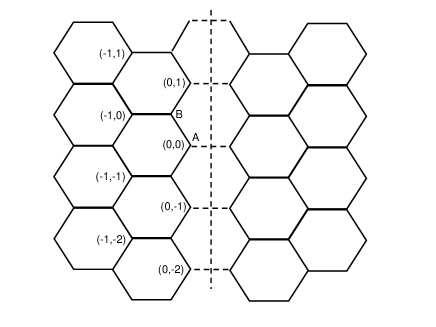
Figure 3: An infinite graphene plane is separated into two halves by adding the perturbation $\hat{V}_{g}$, which nullifies the tunneling along the dashed bonds.

The Green function of the infinite plane is diagonal in the quasimomentum representation due to the translation symmetry. We introduce the spinor Bloch functions as $\Psi_{\mathbf{k}}^{T}(\mathbf{N})=\exp(iK_{1}N_{1}+iK_{2}N_{2})(\psi_{A}(\mathbf{k}),\psi_{B}(\mathbf{k}))$, where k is the quasimomentum, $K_{1}=\mathbf{k}\cdot\mathbf{a}_{1}$ and $K_{2}=\mathbf{k}\cdot\mathbf{a}_{2}$ are the projections of the quasimomentum onto $\mathbf{a}_{1}$ and $\mathbf{a}_{2}$, and $\psi_{A/B}$ are the wave function amplitudes on the $A/B$ sublattices. In the quasimomentum representation the (inverse) Green function of an infinite graphene plane can be written as matrix in the $A/B$ sublattice space,

$$G^{-1}_{0,g}(\mathbf{k})=-\gamma_{g}\left(\begin{array}[]{cc}-\varepsilon_{+}&\!1\!+\!e^{iK_{1}}\!+\!e^{-iK_{2}}\!\\ \!1\!+\!e^{-iK_{1}}\!+\!e^{iK_{2}}\!&-\varepsilon_{+}\\ \end{array}\right).$$ (16)

Here $\gamma_{g}$ denotes the nearest neighbor hopping integral in graphene and we introduced the dimensionless energy $\varepsilon_{+}\equiv\epsilon_{+}/\gamma_{g}$.

The Dirac points at the corners of the hexagonal Brillouin zone correspond to $K_{1}=K_{2}=\pm 2\pi/3$. At these points the off-diagonal matrix elements in the above equation vanish. The Hamiltonian near these points reduces to the familiar Dirac equation with the linear spectrum near the Dirac points as shown in Fig. 4.

The perturbation $\hat{V}_{g}$ that cuts the graphene plane into two halves is given by (see Fig. 3),

$$\hat{V}_{g} = \gamma_{g}\delta_{N_{2},N_{2}^{\prime}}\left[u_{g}\,\delta_{N_{1},N_{1}^{\prime}}\left(\begin{array}[]{cc}\delta_{N_{1},0}&0\\ 0&\delta_{N_{1},1}\\ \end{array}\right)\right.$$ (22)

$$-\left.\left(\begin{array}[]{cc}0&\delta_{N_{1},0}\delta_{N_{1}^{\prime},1}\\ \delta_{N_{1},1}\delta_{N_{1}^{\prime},0}&0\\ \end{array}\right)\right].$$

The second matrix in the brackets nullifies electron tunneling between the two halves of the plane, and the first matrix describes the on-site potential for the atoms along the zigzag edge. This potential is parameterized in our model by the dimensionless parameter $u_{g}$, which is equal to the ratio of the on-site potential to the hopping integral $\gamma_{g}$. Because of the diminished number of neighbors for the edge atoms the on-site potential is expected to be positive and have a magnitude of the order of $eV$, i.e. of the same order as the hopping integral, $0<u_{g}\lesssim 1$.

Due to the symmetry of the problem with respect to translations along the edge, $(N_{1},N_{2})\to(N_{1},N_{2}+m)$ the corresponding quasimomentum, $K_{2}$, is conserved. Therefore below we use a mixed position/quasimomentum representation, $(N_{1},K_{2})$.

In this representation the matrix $\hat{V}_{g}$ is independent of $K_{2}$ and has nonzero matrix elements only in the $2\times 2$ space spanned by the states $|A,N_{1}=0\rangle$ and $|B,N_{1}=1\rangle$, which correspond to the carbon atoms on the opposite sides of the divide separating the plane into two halves. In this $2\times 2$ subspace $\hat{V}_{g}$ is given by

$$V_{g}=\gamma_{g}\left(\begin{array}[]{cc}u_{g}&-1\\ -1&u_{g}\\ \end{array}\right).$$ (23)

In this representation the matrix $\hat{V}_{g}$ is independent of $K_{2}$ and has nonzero matrix elements only in the $2\times 2$ space spanned by the states $|A,N_{1}=0\rangle$ and $|B,N_{1}=1\rangle$, which correspond to the carbon atoms on the opposite sides of the divide separating the plane into two halves. In this $2\times 2$ subspace $\hat{V}_{g}$ is given by

$$V_{g}=\gamma_{g}\left(\begin{array}[]{cc}u_{g}&-1\\ -1&u_{g}\\ \end{array}\right).$$ (24)

The reflection amplitude of the junction, Eq. (14), depends only on the Green function of the semi-infinite graphene inside the same $2\times 2$ subspace. In the mixed representation the latter satisfies the equation

$$G_{g}(K_{2})=G_{0,g}(K_{2})+G_{0,g}(K_{2})V_{g}G_{g}(K_{2}),$$ (25)

where the perturbation $V_{g}$ is given by Eq. (24) and $G_{0,g}(K_{2})$ is the unperturbed Green function inside the $2\times 2$ subspace (in the mixed representation). The latter is evaluated in Appendix B and is given by

$$G_{0,g}(K_{2})=\frac{1}{\gamma_{g}\sqrt{ab}}\left(\begin{array}[]{cc}\varepsilon&\!1\!-\!C\!+\!\varepsilon^{2}\!+\!\sqrt{ab}\!\\ \!1\!-\!C\!+\!\varepsilon^{2}\!+\!\sqrt{ab}\!&\varepsilon\\ \end{array}\right),$$ (26)

where we introduced the notations

$$C=4\cos^{2}\frac{K_{2}}{2},\,\,a=(1+\varepsilon)^{2}-C,\,\,b=(1-\varepsilon)^{2}-C.$$ (27)

The branch of $\sqrt{ab}$ in Eq. (26) is determined by analytic continuation of $\varepsilon$ from the positive imaginary axis, where $\sqrt{ab}$ takes positive real values.

Using Eqs. (24), (25) and (26) we obtain

$$G_{g}(K_{2})=\frac{2\sqrt{ab}+(1-u_{g})a+(1+u_{g})b}{\gamma_{g}[(1-u_{g})^{2}a-(1+u_{g})^{2}b]}\left(\begin{array}[]{cc}1&0\\ 0&1\\ \end{array}\right).$$ (28)

The off-diagonal matrix elements in the above expression vanish, as they should due to the absence of tunneling between the two half-planes. The $(1,1)$ matrix element determines the Green function at the zigzag edge for a given quasimomentum $K_{2}$ along the edge. Its imaginary part gives the tunneling density of states into the edge for a given quasimomentum. It arises from two distinct contributions of the edge and bulk states, which we discuss next.

III.2.1 Tunneling density of states into the zigzag edge

The tunneling density of states at the zigzag edge of graphene is described by the imaginary part of the diagonal matrix elements in the Green function Eq. (28). Physically, the density of states at the edge contains the contributions from the bulk and edge states. The contribution of the bulk states is described by the imaginary part of $\sqrt{ab}$ whereas the contribution of the edge states corresponds to the pole at $(1-u_{g})^{2}a-(1+u_{g})^{2}b=0$. This condition defines the spectrum of the edge states,

$$\varepsilon=\frac{1+u^{2}_{g}-\sqrt{(1+u^{2}_{g})^{2}+4u^{2}_{g}(2\cos{K_{2}}+1)}}{2u_{g}}$$ (29)

with $\cos{K_{2}}<-\frac{1}{2}$.

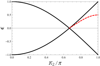
Figure 4: Color online: The solid (black) curve represents the intersection of the bulk state spectrum of graphene with the $K_{1}=2\pi/3$ plane that goes through the Dirac point. The dashed (red) curve represents the spectrum of the edge states, which exist only for $2\pi/3<K_{2}<\pi$. The edge state spectrum lies below the bulk state spectrum.

This spectrum is plotted in Fig. 4. The inequality $\cos{K_{2}}<-\frac{1}{2}$ reflects the fact that for $u_{g}>0$, the edge states exist only for $\varepsilon>0$ as shown in the following text. For $\varepsilon<0$, the density of states for the edge states vanish, or the numerator in Eq. (28) vanishes together with the denominator, eliminating the pole.

For weak on-site potential at the edge, $u_{g}\ll 1$, the edge state spectrum reduces to $\varepsilon=-u_{g}(1+2\cos{K_{2}})$, with $\cos{K_{2}}\leq-\frac{1}{2}$. In this limit the spectrum and the wave functions of the edge states can be understood quite easily. In the absence of the on-site potential at the edge, $u_{g}=0$, these states have wave functions which reside only on the $A$-sublattice and are eigenfunctions of the quasimomentum $\mathbf{k}=(K_{1},K_{2})$. It is easy to see from Eq. (29) that these states form a degenerate band of zero energy states, in agreement with Ref. edge_1996, . From Eq. (16) it follows that in order to obey the Schrödinger equation in the interior of the lead the quasimomentum of such states must satisfy the condition $e^{-iK_{1}}=-1-e^{iK_{2}}$. Further, since the wave function of these states vanishes on the $B$-sublattice they remain eigenstates of the Hamiltonian even after the plane is separated into two halves. The normalizability condition for the edge states is $\mathrm{Im}K_{1}<0$, implying $|1+e^{iK_{2}}|<1$, which is equivalent to the inequality below Eq. (29). And the amplitude of the edge states decay with a factor of $2\cos{(K_{2}/2)}$. For weak on-site potential at the edge, $u_{g}\ll 1$ the edge state spectrum may be obtained from the first order in perturbation, $\varepsilon(K_{2})=u_{g}|\psi_{A}(K_{2})|^{2}$, where $\psi_{A}(K_{2})$ is the wave function of the edge state at the edge atoms. The normalization condition gives $|\psi_{A}(K_{2})|^{2}=1/\sum_{N_{1}=-\infty}^{0}\exp(2N_{1}\mathrm{Im}K_{1})=-(1+2\cos K_{2})$.

The above consideration illustrates that in the presence of the on-site potential at the edge the band of edge states acquires a finite width of order of the on-site potential. For strong on-site potential at the edge perturbation theory is no longer applicable and the spectrum of the edge states is given by Eq. (29). At zero energy the spectrum of these states is linear, which results in the finite density of states. It might seem therefore that at small energies, $\varepsilon\ll 1$, the contribution of the edge states to the tunneling density of states will be much larger than that of the bulk states. This is not so however because at small energies near $K_{2}=2\pi/3$ the wave functions of edge states extend into the bulk over many lattice spacings, so that the local density of such states at the edge vanishes linearly with energy. As a result, for $u_{g}\sim 1$ the contribution of these states to the tunneling DoS at the edge turns out to be of the same order as that of bulk states.

The real space Green function $G_{g}(\textbf{0},\textbf{0})$ at the contact point is obtained by integrating the diagonal element of $G_{g}(K_{2})(\textbf{0},\textbf{0})$ in Eq. (28) over $K_{2}$: $G_{g}(\textbf{0},\textbf{0})=\int\frac{dK_{2}}{2\pi}\,G_{g}(K_{2})$. We write this integral as a contour integral over the unit circle of the variable $z_{2}=\exp(iK_{2})$. Inside the contour the integrand has a simple pole corresponding to the edge states and a branch corresponding to the bulk states. We denote the contribution of the pole and the branch cut by $G_{pole}$ and $G_{bc}$ respectively,

$$G_{g}(\mathbf{0},\mathbf{0})=\frac{1}{\gamma_{g}}(G_{pole}+G_{bc}).$$ (30)

A lengthy but straightforward calculation gives,

$$G_{pole}=-i\frac{|\varepsilon|}{u_{g}}\frac{(1-u^{2}_{g})\theta(\varepsilon)}{\sqrt{3u_{g}^{2}-2u_{g}\varepsilon-\varepsilon^{2}}},$$ (31)

where $\theta(\epsilon)$ is the step function indicating that the density of states due to edge states is present only for $\varepsilon>0$. The contribution of the branch cut, $G_{bc}$, can be evaluated analytically at low energies,

$$G_{bc} = -\frac{1}{3u_{g}}+\frac{\varepsilon}{\pi u_{g}}\frac{(1+u^{2}_{g})}{\sqrt{3u_{g}^{2}-2u_{g}\varepsilon-\varepsilon^{2}}}\log{\frac{2|\varepsilon|}{\sqrt{3(3u_{g}^{2}-2u_{g}\varepsilon-\varepsilon^{2})}+3u_{g}-\varepsilon}}-ic\frac{|\varepsilon|}{u_{g}},$$ (32)

where $c=\frac{1}{2\pi}(1+\frac{\pi}{2}-\frac{2\pi}{3\sqrt{3}})\approx 0.22$. The imaginary parts of both contributions (and with them the tunneling DoS at the edge) vanish linearly with energy at small energy.

III.2.2 Reflection coefficient of the junction at low energies

Substituting the previous Eqs. (30)-(32) into Eq. (14) we obtain a simple expression for the reflection coefficient of the junction at low energies, $|\varepsilon|\ll 1$,

$$|r(\epsilon)|^{2}=1-\eta\varepsilon$$ (33)

with $\eta=-2\sqrt{4-u^{2}_{w}}[(1-u^{2}_{g})/\sqrt{3u_{g}}+c]/(u_{g}+\frac{1}{9u_{g}}-\frac{u_{w}}{3})$. In this regime the electron wave incident from the carbon chain into the junction is almost perfectly reflected.

IV Device conductance at low energies: asymmetric resonances

The strong reflection at the junction at low energies indicates that the transmission coefficient of the whole device in Eq. (2) also tends to vanish at small energies except in the vicinity of resonances, $\cos(2\mathcal{N}k+2\delta_{0})=1$. Substituting $|r_{r/l}(\epsilon)|=|r(\epsilon)|$ from Eq. (33) into Eq. (2) we obtain a simple expression for the transmission coefficient of the device at low energies,

$$\mathcal{T}(\epsilon)=\left[1+\frac{\kappa}{\epsilon^{2}}[1-\cos(2\mathcal{N}k+2\delta_{0})]\right]^{-1}.$$ (34)

Here $\delta_{0}=2\arctan(\gamma/3u)$ is the contact scattering phase shift at zero energy and $\kappa=2/\eta^{2}$, where $\eta$ is a number of order unity defined below Eq. (33).

Expanding the cosine near a resonance energy $\epsilon=\epsilon_{0}$, we obtain a simple expression for the transmission coefficient at small energies,

$$\mathcal{T}(\epsilon)=\left[1+\alpha\left(1-\frac{\epsilon_{0}}{\epsilon}\right)^{2}\right]^{-1},$$ (35)

where $\alpha=\mathcal{N}^{2}\kappa/2$ is a dimensionless parameter. This reproduces the result (3) expected from qualitative considerations in the case of symmetric coupling. The resonance width is $\Gamma\sim\epsilon_{0}/\mathcal{N}$. The resonance shape is strongly asymmetric and markedly different from that of the Breit-Wigner resonance, as shown in Fig. 1.

V Summary and discussion

We studied electron transport through a single atom carbon chain connected to graphene leads. The simplicity of the hybridization pattern of electron orbitals in graphene and carbon chains enabled us to construct an analytically solvable model and thereby gain physical insight into the essential features of electron conduction in the system.

Transmission through the device is dominated by scattering at the contacts between the chain and the lead. For typical temperatures and doping levels in graphene the current-carrying electron states have energies much smaller than the band width. At these energies the contact between the chain and the lead becomes almost perfectly reflecting. Its reflection amplitude can be expressed in terms of the Green’s function, $G_{g}(\mathbf{0},\mathbf{0})$, of the lead at the atomic site connected to the carbon chain, see Eq. (14). In this equation the parameter $\gamma$ describes the strength of coupling between the chain and the lead. At low electron energies the phase factor $e^{ik}$ may be assumed energy independent, as it changes appreciably only at energy scales of order of the band width in the wire. In this regime the energy dependence of the transmission coefficient is dominated by that of the density of states in the lead. For graphene leads it becomes linear, see Eqs. (33) and (1).

For leads with zigzag edges both the bulk and edge states contribute to the DoS at the contact point. Due to the difference in the on-site energy between the atoms at the edge and in the interior of graphene the band of edge states acquires a finite dispersion. The spectrum of this band is given by Eq. (29) and is plotted in Fig. 4. Although the edge state spectrum is linear at small energies its contribution to the local DoS at the edge is not constant, but rather is linear in the electron energy, $\sim\epsilon\theta(\epsilon)$. This occurs because the edge state wave functions extend into the bulk to distances which are inversely proportional $\epsilon$, as explained in Sec. III.2.1. As the difference in the on-site potential between the atoms at the edge and in the interior of the lead is of the same order as the band width the contribution of edge states to the DoS is of the same order as that of the bulk states. Therefore a substantial part of the current through the carbon chain is propagated into the lead by the edge states. The energy dependence of the reflection coefficient of the junction is described by Eq. (33).

The interference between reflection amplitudes of the left and right junctions gives rise to the transmission coefficient of the device described by Eq. (34). Due to the nearly perfect reflection at the contact the energy dependence of the transmission coefficient of the interconnect has resonant character. Near the resonance the transmission coefficient is described by a simple expression, Eq. (35).

Our main conclusions, namely the linear energy dependence of the transmission coefficient of the junction between the chain and the lead and the shape of the resonance in Eq. (35) do not depend on many of the simplifying assumptions of our model.

The linear energy dependence of the junction transmission coefficient holds if the coupling between the chain and the lead is energy independent. This assumption is valid as long as the electron energy is smaller than the inverse propagation time across the contact and holds for more complicated junctions, e.g. a small peninsular connecting the chain to the lead. In this case Eqs. (14) and (34) will still hold, provided $\gamma$ and $\eta$ are replaced by the appropriate parameters describing the coupling strength between the chain and the lead at low energies. Similarly, Eq. (35) will also hold provided the resonance energy and the parameter $\alpha$ are chosen appropriately. The generalization of the resonance shape to the case of asymmetric contacts is given by Eq. (3).

The resonant character of transmission will be preserved even in the presence of the Coulomb interaction in the wire, as long as wire is short enough so that the one-dimensional correlation effects can be neglected. Such a wire will act as a molecule with a single resonant level participating in transport. For longer wires the one-dimensional correlations need to be taken into account. In this respect the Umklapp processes and the formation of Friedel oscillations near the contact points are especially important. The study of these effects is left for future work.

We are grateful to M. Bockrath, D. Cobden, J. Lau, J. Rehr, and B. Spivak for useful discussions. This work was supported by the DOE grants DE-FG02-07ER46452 (W.C. and A.V.A.) and DE-FC02-00ER41132 (G.F.B.).

Appendix A Green function of a semi-infinite wire

We construct the Green function of the semi-infinite wire from that of the infinite wire by adding a perturbation that nullifies the hopping between the two halves.

The retarded Green function of the infinite wire in $k$ space is diagonal and given by

$$G_{0,w}(k)=(\epsilon-\epsilon_{k}+i0)^{-1}$$ (36)

with

$$\epsilon_{k}=u_{w}\gamma_{w}+2\gamma_{w}\cos k.$$ (37)

The real space Green function is obtained by integrating over $k$ as

$$G_{0}(n,n^{\prime})=\frac{1}{2\pi}\int dkG_{0,w}(k)e^{ik(n-n^{\prime})}$$ (38)

which gives

$$G_{0,w}(n,n^{\prime})=\frac{1}{2i\gamma_{w}\sin k}\exp(-ik|n-n^{\prime}|)$$ (39)

where $k$ is the magnitude of the electron quasimomentum related to the energy by $\epsilon=u_{w}\gamma_{w}+2\gamma_{w}\cos k$.

The perturbation $\hat{V}_{w}$ which cuts the wire to two halves has non-vanishing matrix elements only in the $2\times 2$ subspace spanned by the orbitals with $n=0$ and $n=1$, where it is given by

$$\left(\begin{array}[]{cc}V_{w}(0,0)&V_{w}(0,1)\\ V_{w}(1,0)&V_{w}(1,1)\\ \end{array}\right)=-\left(\begin{array}[]{cc}0&\gamma_{w}\\ \gamma_{w}&0\\ \end{array}\right).$$ (40)

The $T$ matrix defined in Eq. (8) is also nonvanishing only in the $2\times 2$ subspace and can be expressed solely in terms of the matrix elements of $\hat{G}_{0,w}$ in the $2\times 2$ space,

$$\left(\begin{array}[]{cc}G_{0,w}(0,0)&G_{0,w}(0,1)\\ G_{0,w}(1,0)&G_{0,w}(1,1)\\ \end{array}\right)=\frac{1}{2i\gamma_{w}\sin k}\left(\begin{array}[]{cc}1&e^{-ik}\\ e^{-ik}&1\\ \end{array}\right).$$ (41)

Using Eqs. (39), (40), (41), (7) and (8) we obtain the Green function of the semi-infinite wire, Eq. (13).

Appendix B Derivation of Eq. (26)

In this appendix we derive the expression for the unperturbed graphene Green function within the $2\times 2$ subspace spanned by the rows of atoms on the opposite sides of the dashed links in Fig. 3.

The unperturbed Green function in the quasimomentum representation is obtained by inverting the matrix in Eq. (16),

$$G_{0,g}(\mathbf{k})=-\frac{1}{D}\left(\begin{array}[]{cc}-\varepsilon&\!1\!+\!e^{iK_{1}}\!+\!e^{-iK_{2}}\!\\ \!1\!+\!e^{-iK_{1}}\!+\!e^{iK_{2}}\!&-\varepsilon\end{array}\right),$$

where $D=\gamma_{g}\left[\varepsilon^{2}-(\!1\!+\!e^{-iK_{1}}\!+\!e^{iK_{2}}\!)(\!1\!+\!e^{iK_{1}}\!+\!e^{-iK_{2}}\!)\right]$.

In the mixed representation the Green function $\hat{G}_{0,g}(K_{2})$ in the $2\times 2$ subspace of states $|A,N_{1}=0\rangle$ and $|B,N_{1}=1\rangle$, can be obtained by the inverse Fourier transform of $G_{0,g}(\mathbf{k})$ with respect to $K_{1}$. An elementary calculation gives

$$\langle A,0|\hat{G}_{0,g}(K_{2})|A,0\rangle=\langle B,1|\hat{G}_{0,g}(K_{2})|B,1\rangle$$

$$=\int\frac{dK_{1}}{2\pi}\frac{\varepsilon}{D}=\frac{\varepsilon}{\gamma_{g}\sqrt{ab}},$$ (42)

and

$$\langle A,0|\hat{G}_{0,g}(K_{2})|B,1\rangle=\langle B,1|\hat{G}_{0,g}(K_{2})|A,0\rangle^{*}$$

$$=-\int\frac{dK_{1}}{2\pi}\frac{1\!+\!e^{iK_{1}}\!+\!e^{-iK_{2}}}{D}e^{-iK_{1}}$$

$$=\frac{1}{\gamma_{g}\sqrt{ab}}\left[1-C+\varepsilon^{2}+\sqrt{ab}\right],$$ (43)

where $a$, $b$ and $C$ are defined in Eq. (27).

Combining the above matrix elements into one $2\times 2$ matrix we arrive at Eq. (26).

References

- (1) M. A. Reed, C. Zhou, C. J. Muller, T. P. Burgin, and J. M. Tour, Conductance of a molecular junction. Science 278, 252 (1997).
- (2) J. Chen, M. A. Reed, A. M. Rawlett, and J. M. Tour, Science 286, 1550 (1999).
- (3) H. Park, J. Park, A.K.L. Lim, E.H. Anderson, A.P. Alivisatos, and P.L. McEuen, Nature 407, 57 (2000).
- (4) J. Park et al., Nature 417, 722 (2002).
- (5) W. Liang et al., Nature 417, 725 (2002).
- (6) N. Agrait, A. L. Yeyati, J. M. van Ruitenbeek, Physics Reports, 377, 81, (2003).
- (7) P. L. McEuen, Nature 393, 15 (1998).
- (8) S. Iijima, Nature 354, 56 (1991).
- (9) K. S. Novoselov, A. K. Geim, S. V. Morozov, Science 306, 666 (2004).
- (10) N. D. Lang, and Ph. Avouris Phys. Rev. Lett. 81, 3515 (1998).
- (11) G. Cuniberti, G. Fagas, and K. Richter, J. Chem. Phys. 281, 465 (2002).
- (12) T.D. Yuzvinsky, W. Mickelson, S. Aloni, G. E. Begtrup, A. Kis, A. Zettl, Nano Lett. 6 2718(2006).
- (13) K.H. Khoo, J.B. Neaton, Y.W. Son, M.L. Cohen, and S.G. Louie, Nano Letters 8 2900 (2008).
- (14) B. Standley, W. Bao, H. Zhang, J. Bruck, C. N. Lau, and M. Bockrath, Nano Letters 8, 3345 (2008).
- (15) C. Jin, H. Lan, L. Peng, K. Suenaga and S. Iijima, Phys. Rev. Lett. 102, 205501(2009)
- (16) B. Larade, J. Taylor, H. Mehrez and H. Guo, Phys. Rev. B., 64, 075420(2001).
- (17) S. Tongay, R.T. Senger, S. Dag, and S. Ciraci, Phys. Rev. Lett. 93, 136404-1(2004).
- (18) Z. Crljen and G. Baranovic, Phys. Rev. Lett., 98, 116801(2007).
- (19) M. Fujita, K. Wakabayashi, K. Nakada, and K. Kosukabe, J. Phys. Soc. Jap. Lett., 7, 1920 (1996).
- (20) K. Nakada, M. Fujita, G. Dresselhaus, and M. S. Dresselhaus, Phys. Rev. B 54, 17954(1996).
- (21) L.D. Landau and E.M. Lifshitz, Quantum Mechanics (non-relativistic theory), , Butterworth-Heinemann (Oxford, 1997).
- (22) S.Okano and D. Tomanek, Phys. Rev. B 75, 195409(2007)
- (23) G. Seelig and K. A. Matveev, Phys. Rev. Lett. 90, 176804 (2003).
- (24) G. Seelig, K. A. Matveev, and A. V. Andreev, Phys. Rev. Lett. 94, 066802 (2005).