The optical/X-ray connection: ICM iron content and galaxy optical luminosity in 20 galaxy clusters

Abstract

X-ray observations of galaxy clusters have shown that the intra-cluster gas has iron abundances of about one third of the solar value. These observations also show that part (if not all) of the intra-cluster gas metals were produced within the member galaxies. We present a systematic analysis of 20 galaxy clusters to explore the connection between the iron mass and the total luminosity of early-type and late-type galaxies, and of the brightest cluster galaxies (BCGs). From our results, the intra-cluster medium (ICM) iron mass seems to correlate better with the luminosity of the BCGs than with that of the red and blue galaxy populations. As the BCGs cannot produce alone the observed amount of iron, we suggest that ram-pressure plus tidal stripping act together to enhance, at the same time, the BCG luminosities and the iron mass in the ICM. Through the analysis of the iron yield, we have also estimated that SN Ia are responsible for more than 50% of the total iron in the ICM. This result corroborates the fact that ram-pressure contributes to the gas removal from galaxies to the inta-cluster medium, being very efficient for clusters in the temperature range $2<kT$ (keV) $<10$.

1 Introduction

The detection of the Fe line from the X-ray spectral analysis of the intra-cluster medium (ICM; Mitchell et al. 1976; Serlemitsos et al. 1977) indicates that it does not have a primordial chemical composition but was enriched with material processed in stars. The relative importance of the mechanisms that transport metal rich gas to the ICM is not well known. The measurement of heavy element abundances in the ICM can provide important clues on the chemical evolution inside galaxy clusters.

Difficulties in determining the nature of metal enrichment in clusters are enhanced by the variety of astrophysical processes and spatial scales involved: yields from different supernova (SNe) types, the role of galactic winds (e.g., Dupke & White 2000), ram-pressure (e.g., Gunn & Gott 1972) and tidal stripping (e.g., Toomre & Toomre 1972) as mechanisms of metal transport from galaxies to the ICM, star formation efficiency, and the influence of the environment, among other issues.

An important step in clarifying this problem was taken by Arnaud et al. (1992). These authors investigated the correlations between some properties of the ICM, like the gas mass, with the optical luminosity in clusters, finding that the gas mass correlates well with the luminosity of E+S0 galaxies but not with the luminosity of spirals. For a sample of 6 clusters with measured iron abundances and at low redshift, they also found a good correlation between the iron mass and the luminosity of red galaxies (E+S0). They then concluded that ellipticals and lenticulars are dominant in enriching the ICM, indicating that the proto-galactic winds driven by type II SNe at the early stages of cluster formation play a major role in the ICM metal enrichment. Another relevant enrichment mechanism is ram-pressure stripping (hereafter RPS, Gunn & Gott 1972). Current observations indicate that RPS is more common than previously believed, acting also in low density environments such as poor groups and in the outskirts of clusters (Solanes et al. 2001; Kantharia et al. 2005; Levy et al. 2007; Kantharia et al. 2008). This is also supported by recent numerical simulations (e.g., Vollmer et al. 2005; Hester 2006; Brüggen & De Lucia 2008). Ram-pressure stripped gas is more enriched by SN Ia ejecta and can continuously provide an inflow of iron to the ICM through the cluster history (Renzini et al. 1993).

Although the ICM metal enrichment problem has been addressed in many studies (Thielemann et al. 1990; Mushotzky et al. 1996; Mushotzky & Loewenstein 1997; Dupke & White 2000, among others), there are good reasons to revisit it. Firstly, Arnaud et al. (1992) used a limited sample (the only 6 available clusters with masses and luminosities in the literature). Secondly, we are now in the era of precision abundances determination given the superior ability for spatially resolved spectroscopy of the instruments on board of XMM-Newton, Chandra and Suzaku. Finally, there are currently a number of studies, providing ICM physical parameters from large cluster samples homogeneously determined (e.g., Zhang et al. 2007; Maughan et al. 2008).

To readdress this question, we investigate in this work the relation between the metallicity (iron abundance) of the intra-cluster gas and some optical properties of galaxy clusters, in search for clues on how metals got into the ICM.

The outline of the paper is as follows: in Sect. 2 we describe the sources of the data analyzed. In Sect. 3 we present the photometric analysis, describing the separation between the red and blue populations and the determination of their total luminosity. Influence of the Butcher-Oemler effect is also discussed in this section. In Sect. 4 we discuss the dominant population in the iron enrichment by means of the correlation between the iron mass and the total luminosity of the different populations, the mechanism responsible for the metal transport from galaxies to the ICM and the role of SN II and SN Ia. Finally, we present our conclusions in Sect. 5.

2 The Data

We describe in this section the X-ray and optical data used in our analysis.

2.1 X-ray Data

Maughan et al. (2008) carried out an X-ray analysis of a homogeneous sample of 115 galaxy clusters in the redshift range $0.1<z<1.3$. The sample was assembled from publicly available Chandra data and selected in order to ensure cluster emission detection up to $r_{500}$ (the radius within which the cluster mean density exceeds the critical value by a factor of 500), allowing cluster properties to be directly measured up to this radius. We have selected a subsample of galaxy clusters that were analyzed by Maughan et al. (2008) and observed by the Sloan Digital Sky Survey (SDSS, York et al. 2000). Out of 115 clusters 20 were selected (Table 1), and will be the object of the analysis presented in this paper. All the X-ray data used here (metallicity, gas mass and temperature) are taken from Maughan et al. (2008) and are also presented in Table 1.

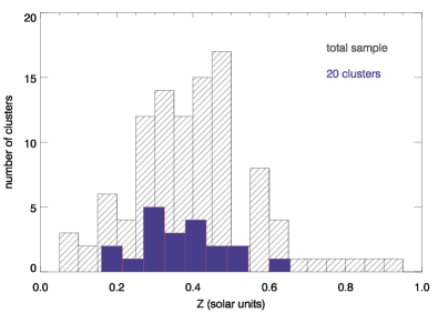
Figure 1: Distribution of iron abundance determined within $r_{500}$ for our selected sub-sample (in dark blue) and for the whole sample analyzed by Maughan et al. (2008) (filled with dashed lines). Our mean value is $Z=(0.34\pm 0.15)Z_{\odot}$, while the average mean for the whole sample is $Z=(0.39\pm 0.14)Z_{\odot}$

In order to check if the 20 clusters analyzed in this work are a fair sample of the original one, we present in Fig. 1 the metallicity (iron abundance) for all the clusters studied by Maughan et al. (2008). The mean metallicity value ($Z=(0.34\pm 0.15)Z_{\odot}$) obtained for our selected sub-sample agrees well with the mean value ($Z=(0.39\pm 0.14)Z_{\odot}$) obtained for the original 115 clusters.

Table 1: Clusters from Maughan et al. (2008) data sample which were observed by SDSS and have X-ray flux high enough for the analysis presented here. Column (1): cluster name; Col. (2): right ascension; Col. (3): declination; Col. (4): redshift; Col. (5): $r_{500}$ radius; Col. (6): mean temperature derived from the X-ray emission within $r_{500}$; Col. (7): mean metallicity inside within $r_{500}$; Col. (8): gas mass within $r_{500}$.

Cluster	R.A	DEC	z	$r_{500}$	$<kT>$	$<Z>$	$M_{gas}$
	(J2000)	(J2000)		($h_{70}^{-1})$ Mpc	(keV)		$10^{13}M_{\odot}$
A267	01:52:42.12	+01:00:41.4	0.230	1.04	$4.9_{-0.3}^{+0.3}$	$0.49_{-0.17}^{+0.18}$	$5.74_{-0.07}^{+0.10}$
MS0906.5+1110	09:09:12.72	+10:58:33.6	0.180	1.06	$5.3_{-0.2}^{+0.2}$	$0.31_{-0.07}^{+0.07}$	$5.27_{-0.04}^{+0.05}$
A773	09:17:52.80	+51:43:40.4	0.217	1.25	$7.4_{-0.3}^{+0.3}$	$0.48_{-0.06}^{+0.06}$	$9.09_{-0.06}^{+0.06}$
MS1006.0+1202	10:08:47.52	+11:47:40.6	0.221	1.11	$5.9_{-0.4}^{+0.4}$	$0.16_{-0.10}^{+0.10}$	$5.29_{-0.06}^{+0.06}$
A1204	11:13:20.40	+17:35:39.1	0.171	0.92	$3.4_{-0.1}^{+0.1}$	$0.37_{-0.05}^{+0.05}$	$3.10_{-0.06}^{+0.21}$
A1240	11:23:37.68	+43:05:44.5	0.159	0.92	$3.9_{-0.3}^{+0.3}$	$0.19_{-0.09}^{+0.10}$	$2.75_{-0.03}^{+0.04}$
A1413	11:55:18.00	+23:24:17.6	0.143	1.26	$7.2_{-0.2}^{+0.2}$	$0.41_{-0.03}^{+0.03}$	$7.95_{-0.05}^{+0.04}$
A1682	13:06:51.12	+46:33:29.5	0.234	1.13	$6.2_{-0.8}^{+0.8}$	$0.42_{-0.25}^{+0.27}$	$7.07_{-0.12}^{+0.13}$
A1689	13:11:29.52	-01:20:30.4	0.183	1.37	$9.0_{-0.3}^{+0.3}$	$0.42_{-0.04}^{+0.04}$	$11.26_{-0.06}^{+0.11}$
A1763	13:35:18.24	+40:59:59.3	0.223	1.32	$7.8_{-0.4}^{+0.4}$	$0.29_{-0.07}^{+0.07}$	$11.47_{-0.07}^{+0.10}$
A1914	14:26:01.20	+37:49:35.4	0.171	1.37	$9.8_{-0.3}^{+0.3}$	$0.34_{-0.05}^{+0.05}$	$10.69_{-0.07}^{+0.09}$
A1942	14:38:22.08	+03:40:06.2	0.224	0.94	$4.3_{-0.2}^{+0.3}$	$0.27_{-0.08}^{+0.08}$	$3.59_{-0.03}^{+0.03}$
RXJ1504-0248	15:04:07.44	-02:48:18.4	0.215	1.34	$6.8_{-0.2}^{+0.2}$	$0.35_{-0.04}^{+0.04}$	$10.9_{-0.47}^{+0.04}$
A2034	15:10:12.48	+33:30:28.4	0.113	1.22	$6.7_{-0.2}^{+0.2}$	$0.38_{-0.04}^{+0.04}$	$6.88_{-0.03}^{+0.02}$
A2069	15:24:09.36	+29:53:10.0	0.116	1.20	$6.3_{-0.2}^{+0.2}$	$0.29_{-0.05}^{+0.05}$	$6.56_{-0.03}^{+0.03}$
A2111	15:39:41.28	+34:25:10.2	0.229	1.18	$6.8_{-0.5}^{+0.9}$	$0.23_{-0.15}^{+0.15}$	$7.44_{-0.05}^{+0.10}$
RXJ1701+6414	17:01:23.04	+64:14:11.4	0.225	0.93	$5.2_{-0.4}^{+0.6}$	$0.60_{-0.17}^{+0.18}$	$4.21_{-0.06}^{+0.028}$
A2259	17:20:08.64	+27:40:09.8	0.164	1.09	$5.6_{-0.4}^{+0.4}$	$0.28_{-0.10}^{+0.11}$	$5.29_{-0.07}^{+0.08}$
RXJ1720.1+2638	17:20:10.08	+26:37:29.3	0.164	1.24	$6.1_{-0.1}^{+0.1}$	$0.48_{-0.03}^{+0.03}$	$7.46_{-0.01}^{+0.31}$
RXJ2129.6+0005	21:29:40.08	+00:05:19.6	0.235	1.20	$5.6_{-0.3}^{+0.3}$	$0.50_{-0.10}^{+0.10}$	$8.02_{-0.14}^{+0.14}$

2.2 SDSS data

The photometric data used in our analysis comes from SDSS Data Release 5 (DR5, Adelman-McCarthy et al. 2007), which contains spectroscopic and photometric data for a large number of galaxies observed within almost a quarter of the sky.

In order to investigate the correlation between X-ray properties and galaxy populations, we have selected from the SDSS data galaxies brighter than $r=22$ (extracted from GALAXY tables, which has primary objects subset with type “galaxy”) and within the $r_{500}$ radius of each cluster centre (adopted as the X-ray centre from Maughan et al. 2008). This magnitude limit ensures a significant number of objects for the galaxy population analysis. In this study we will adopt the $(g-r)$ colour, from the DERED tables which are tables of magnitudes already corrected for galactic extinction.

We have also downloaded the same type of data in an annular control field around each cluster (see Section 3), for the statistical subtraction of foreground/background galaxies.

3 Photometric analysis

Since the number of galaxies with measured redshifts in the field of each cluster is small, we have adopted a statistical approach, based on the analysis of the colour-magnitude diagram (CMD) of each cluster, to estimate some properties of the cluster galaxies.

We present in Fig. 2 the $(g-r)$ versus $r$  CMD of A2034 for all galaxies within $r_{500}$. Early-type galaxies in clusters present a tight correlation between their optical colours and luminosity, known as colour-magnitude relation or red-sequence (RS), which is very useful for their identification. In general, galaxies significantly above the red sequence are in the cluster background (since they are redder than the reddest cluster galaxies). We call blue galaxies those below the red sequence (see Fig. 2), which comprise clusters and non-clusters members.

We have used the control fields to obtain the field contamination and the correction required to estimate the numbers and luminosities of cluster galaxies. The procedure we adopt is the following: the first step is to determine, for each field, the position of the red sequence. Bower et al. (1992), Gladders et al. (1998) and Romeo et al. (2008), among others, have shown that the slope of the red sequence in CMDs is almost constant up to redshift $z=0.5$. For this reason, given that all clusters in our sample have redshifts well below this value, we assume that this slope is the same for all clusters in Table 1. Thus, we have used the CMDs of the 5 clusters of our sample (MS0906.5+1110, A2034, A2069, A2259 and RXJ1720.1+2638) with the most prominent red sequence to estimate this slope through a linear fit, obtaining $\sim-0.055$ (see Fig. 2).

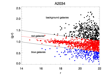
Figure 2: Color-magnitude diagram for galaxies inside $r_{500}$ for A2034, divided in the three groups discussed in the text: red, blue and background galaxies.

For all clusters, we fitted the red sequence as a function of r-band magnitude according to

$$(g-r)=-0.055~{}r+A,$$ (1)

to obtain the zero-point coefficient ($A$). Then, in each cluster, we divided the galaxies in three groups:

• red galaxies: those galaxies within 0.3 mag (De Lucia & Poggianti 2008) from the best fit color-magnitude relation. That is $(g-r)\pm 0.3$ mag zone.

• blue galaxies: galaxies bluer than the $(g-r)-0.3$ mag. This group contains mainly star-forming galaxies, both in the cluster and in the field.

• background galaxies: galaxies redward of the upper limit of the red sequence. We assume that these galaxies are not cluster members.

We estimate the cluster contamination by background/foreground galaxies using a control field around the cluster defined as an annular region between $7\times r_{500}$ and $8\times r_{500}$ from the cluster centre. This region is far enough from the centre to allow the estimation of background densities, as shown in Fig. 3. We used the CMDs of the galaxies in the control fields to estimate the background contamination (in the number of galaxies and luminosity) for red and blue galaxies in the cluster. The CMDs for the clusters in our sample are shown in Fig. 4.

Figure 3: Galaxy counts distribution as a function of the mean radius of each annulus, given as a function of $r_{500}$, for A1689. The background is estimated from the annuli with $R\geq 7\times r_{500}$.

For each bin of magnitude, the number count of galaxies is given by:

$$N_{\rm cl}(m)=N_{\rm cl+bkg}(m)-\gamma N_{\rm bkg}(m),$$ (2)

where $N_{\rm cl}(m)$ is the expected number of cluster galaxies at a certain magnitude interval, $N_{\rm cl+bkg}(m)$ is the total number of galaxies along the line of sight in the same magnitude interval, $N_{\rm bkg}(m)$ is the number of background and foreground galaxies in the same magnitude interval, $\gamma$ is the ratio between cluster and control field areas, and $m$ is the mean magnitude of the interval. After subtracting the background and foreground contamination, cluster counts per magnitude bin in the $r$ band were determined and converted to luminosity.

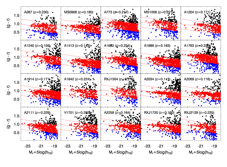
Figure 4: Colour-magnitude diagrams within $r_{500}$ for the 20 clusters in our sample.

3.1 Luminosity of the brightest galaxies

The division of our sample in groups described above enable us to calculate separately the total luminosity of the red and the blue population. We obtained the $r$-band luminosity of the brightest cluster galaxies (BCGs), $L_{BCG}$, directly from the SDSS.

We used the distance modulus given by:

$$M_{r}=m_{r}-25-5\log(d_{\rm L}/\rm 1Mpc)-k(z),$$ (3)

where $d_{L}$ is the luminosity distance (computed assuming $\Omega_{m}=0.3$, $\Omega_{\lambda}=0.7$, and $h=0.7$) and $k$(z) is the $k$-correction computed by Poggianti (1997). Converting magnitudes to luminosities we integrated the luminosity function in order to obtain the total luminosity for each population. These luminosities are given in Table 2.

Table 2: Properties derived from optical data. Column (1): cluster name; Col.(2): total luminosity of the red population within $r_{500}$; Col.(3): total luminosity of the blue population within $r_{500}$; Col.(4): luminosity of BCGs; Col.(5): iron mass derived from Eq. 4 within $r_{500}$.

Cluster	$L_{red}$	$L_{blue}$	$L_{BCG}$	$M_{Fe}$
	($10^{12}L_{\odot}$)	($10^{12}L_{\odot}$)	($10^{11}L_{\odot}$)	($10^{11}M_{\odot}$)
A267	2.19 $\pm$ 0.03	1.82 $\pm$ 0.01	1.84	0.52 $\pm$ 0.18
MS0906.5+1110	2.69 $\pm$ 0.05	1.00 $\pm$ 0.01	0.92	0.30 $\pm$ 0.06
A773	3.82 $\pm$ 0.07	2.08 $\pm$ 0.01	0.68	0.80 $\pm$ 0.10
MS1006.0+1202	1.85 $\pm$ 0.05	1.45 $\pm$ 0.01	1.22	0.16 $\pm$ 0.09
A1204	0.66 $\pm$ 0.02	0.74 $\pm$ 0.02	0.54	0.21 $\pm$ 0.03
A1240	0.79 $\pm$ 0.02	0.73 $\pm$ 0.07	0.13	0.10 $\pm$ 0.05
A1413	0.79 $\pm$ 0.04	0.83 $\pm$ 0.01	1.71	0.60 $\pm$ 0.04
A1682	2.9 $\pm$ 0.08	2.34 $\pm$ 0.02	0.94	0.54 $\pm$ 0.32
A1689	2.31 $\pm$ 0.04	1.21 $\pm$ 0.07	0.76	0.87 $\pm$ 0.01
A1763	3.21 $\pm$ 0.02	2.18 $\pm$ 0.03	0.83	0.61 $\pm$ 0.02
A1914	1.77 $\pm$ 0.03	0.92 $\pm$ 0.04	0.46	0.67 $\pm$ 0.09
A1942	2.22 $\pm$ 0.08	1.44 $\pm$ 0.01	0.89	0.18 $\pm$ 0.05
RXJ1504-0248	1.66 $\pm$ 0.04	1.35 $\pm$ 0.08	1.66	0.70 $\pm$ 0.05
A2034	0.53 $\pm$ 0.02	0.35 $\pm$ 0.06	0.87	0.48 $\pm$ 0.05
A2069	0.89 $\pm$ 0.04	0.34 $\pm$ 0.04	0.41	0.35 $\pm$ 0.06
A2111	4.16 $\pm$ 0.02	2.06 $\pm$ 0.02	0.54	0.31 $\pm$ 0.20
RXJ1701+6414	2.02 $\pm$ 0.05	1.59 $\pm$ 0.01	0.06	0.46 $\pm$ 0.16
A2259	0.92 $\pm$ 0.05	1.02 $\pm$ 0.07	1.22	0.27 $\pm$ 0.09
RXJ1720.1+2638	1.13 $\pm$ 0.03	0.94 $\pm$ 0.07	1.23	0.66 $\pm$ 0.38
RXJ2129.6+0005	2.15 $\pm$ 0.01	2.08 $\pm$ 0.02	1.15	0.73 $\pm$ 0.14

3.2 Butcher-Oemler effect

In a hierarchical scenario clusters grow through the accretion of galaxies and groups, most of them containing blue galaxies. Indeed, many blue galaxies in clusters may be considered newcomers (e.g., Sodré et al. 1989) and, through effects suffered in the hostile environment of galaxy clusters, most of their ISM gas ends up being transferred to the ICM, contributing to its chemical enrichment. We call attention to the fact that the time-scale of colour (spectral) evolution is shorter than that of the morphological evolution (Goto et al. 2004), meaning that some passive spiral galaxies through their evolution may be observed as red objects.

An observational evidence of the hierarchical scenario is the Butcher-Oemler (BO) effect (Butcher & Oemler 1984). We have noticed that this effect can be detected with our data (and has been previously detected by Rakos & Schombert 1995; Margoniner & de Carvalho 2000) and Figure 5 shows that this trend can be detected even in low redshift clusters. We define the fraction of blue galaxies as the ratio between the number of blue (see Sect. 3) to total number of galaxies in a cluster after background correction, indicating an extremely rapid change in the fraction of blue galaxies from $\sim 10\%$ to more than $30\%$ at only $z\sim 0.25$. In contrast, evolutionary models for passive evolution of simple stellar populations predict that colour changes were not as dramatic as found here (Rakos & Schombert 1995).

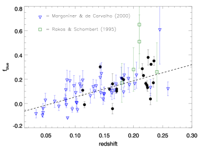
Figure 5: Spiral fraction as a function of redshift. The dashed line is our best-fit for this sample. The filled circles are the sample analyzed i n this work, while the green points were taken from Rakos & Schombert (1995) and the upside down blue triangle are taken from Margoniner & de Carvalho (2000) for this redshift interval.

4 The iron content/optical light connection in 20 galaxy clusters

In this section we investigate the links between the iron content and the luminosities of the red and blue populations of each cluster.

4.1 The iron mass and its relation to the luminosity of the galaxy populations within $r_{500}$

In clusters, there is a number of emission lines over the continuum bremsstrahlung spectrum, the most prominent being those in the iron complex at $\sim$ 7 keV. X-ray observations, have revealed the presence of heavy elements in the ICM, providing direct evidence that this gas was enriched by metals processed by stars (e.g., Mitchell et al. 1976; David et al. 1991; Mushotzky et al. 1996). Studies of large samples of clusters have shown that the Fe abundance is distributed around a value of 0.3 solar (Mushotzky & Loewenstein 1997; Allen & Fabian 1998; Tozzi et al. 2003; Ettori 2005), which is consistent with the mean value of our sample, $Z=0.34\pm 0.15$.

The metallicity derived from X-ray spectra is emission-weighted, so that the values from the central regions tend to overpower global spectral fittings. Therefore, a single global abundance value may lead to erroneous results when associating metals to galaxy luminosities in the whole cluster. Chandra’s excellent spatial resolution is a greatly advantageous over previous satellites for this analysis for intermediate redshift clusters because it can separate the inner and outer regions extremely well (not including projection effects), so that accurate average abundances out of the cooling core region can be measured, making our analysis more realistic. While Arnaud et al. (1992) used one single value for abundances, we are using two different values (one for the internal regions, within $0.15~{}r_{500}$, and one for the annulus $0.15~{}r_{500}<r<r_{500}$), and the results are very similar (section 4.2). Naturally, one single value for the outer abundances is still susceptible to the above mentioned biases, but there were simply not enough photons to subdivide the outer regions in several annuli and still have abundances with satisfactory significance.

In the present work, the iron mass of each cluster enclosed within $r_{500}$ was estimated as the product of the iron abundance by the gas mass and by the solar photospheric abundance by mass (0.00197; Anders & Grevesse 1989):

$$M_{Fe}=M_{\rm gas}(<r_{500})~{}\times~{}Z~{}\times~{}0.00197,$$ (4)

where $M_{\rm gas}$ is the gas mass and $Z$ is the metallicity, both computed within $r_{500}$.

Eq.(4) gives the relation between the iron mass in the ICM and the gas mass for our sample. The iron mass is consistent with a linear scaling with the gas mass, which is expected if $Z_{Fe}\approx$ constant.

To explore what is the dominant population responsible for the metal enrichment in galaxy clusters we show, in Fig. 6, the dependence of the iron mass with the luminosity of red, blue and BCG galaxies. Given the large scatter observed, we adopt the robust Spearman correlation coefficient $\rho$ and the null probability (NP; i.e, the probability of failing to reject the null hypothesis) to evaluate the significance of the correlations (see Press et al. 1992). We obtain $\rho$ values equal to 0.021 (NP=92%), 0.15 (NP=52%) and 0.41 (NP=8%) for the red, blue and BCG galaxies, respectively. The statistical significance of the correlations between luminosities of different populations and ICM iron mass is very low, as seen in Fig. 6. Figures 6 show that all the correlations are very poor and it is not obvious that a given galaxy population is more significantly correlated with the iron mass than the others. To address this question, we adopted a bootstrap resampling technique to estimate for what fraction of a sample a correlation is better than another in the sense that it has a larger Spearman rank-order coefficient $\rho$ (Press et al. 1992). We found that the correlation between the iron mass and BCG luminosities is better than that with the luminosities of the red galaxies at the 90% confidence level and of the blue population at the 85% confidence level. We also found that the significance of the correlations between the blue and red populations with iron mass are barely distinguishable and, in consequence, we cannot draw any firm conclusion about the relative importance of these two populations in the ICM iron enrichment.

Figure 6: Left panel: iron content as a function of total luminosity for red galaxies. Middle panel: iron content as a function of total luminosity for blue galaxies. Right panel: iron content as a function of BCG luminosities. The regression line has a slope of $\alpha=0.75$. The 1$\sigma$ error on $\alpha$ is $\pm$ 0.33

Our results do not confirm the classic idea where early-type galaxies play the major role in the ICM enrichment (Arnaud et al. 1992). Arnaud et al. (1992) included the BCGs in their ‘E+S0’ sample and, from our work, we find that when they are excluded from the red population, the correlation between the red galaxies and the iron mass becomes significantly worse (indistinguishable from the blue galaxies). The most prominent correlation is that between the iron mass and the BCGs luminosities. Note that their best fit for the iron mass as a function of the ‘E+S0’ luminosities has a slope of $\alpha=1.0\pm 0.25$, which is, given the uncertainties, consistent with the poor correlation obtained here between the BCGs and the iron mass. Including the BCGs in the sample of red galaxies changes the correlation coefficient between the total galaxy luminosity and the iron mass from $\rho$=0.021 to $\rho$=0.31, closer to that found for BCGs alone, as expected for the case of contamination by the BCGs.

Since the iron mass scales with the gas mass and with the Fe abundance, we plot separately the relations between the metallicities (see upper panels of Fig. 7) and gas masses (see botton panels of Fig. 7) versus the optical galaxy luminosities. From these figures, we still have low statistical corelations but the ones between the BCGs luminosities and either the gas mass or the metallicity are somewhat more visible than the others. We obtained correlation coefficients equal to $\rho$=0.075, $\rho$=0.17 and $\rho$=0.26 for the metallicity and the luminosities of the red, blue and BCGs galaxies, respectively. For the correlations between the gas mass and the luminosities, we obtained $\rho$=0.31, $\rho$=0.21 and $\rho$=0.33 for the red, blue and BCG population, respectively. The slightly better correlation of gas mass with $L_{red}$ (as opposed to $L_{blue}$) is consistent with the enhancement of the fraction of elliptical galaxies with richness (Dressler 1980), given the somewhat high temperature range of our sample (T $>$ 3.4 keV).

Figure 7: Upper panels: Fe abundance within $r_{500}$ as a function of the total luminosity of the red galaxies (left panel), total luminosity of the blue galaxies (middle panel) and as a function of the BCG luminosities (right panel). Botton panels: gas mass as a functions of the total luminosity of the red galaxies (left panel), total luminosity of the blue galaxies (miidle panel) and as a function of the BCG luminosities. We do not found any significant trend in these panels

4.2 The iron mass and its relation with the luminosity of the galaxy populations within an external annulus

De Grandi et al. (2004) found that the iron mass associated to abundance excess which is normally found at the center of cool-core clusters can be entirely produced by the BCGs. In order to take into account possible biases due to contamination by cool core processes, we present here the same correlations computed within an external annulus, (0.15-1)$r_{500}$, to exclude the inner parts.

The iron mass of each cluster enclosed within $(0.15<r<1)R_{500}$, was estimated from Eq. (4) and the gas mass was computed as,

$$M_{\rm gas}=\int_{0.15r_{500}}^{r_{500}}\kern-15.00002pt\rho_{g}4\pi{r^{\prime}}^{2}\mathrm{d}r^{\prime}=4\pi m_{H}\overline{Z}\int_{0.15r_{500}}^{r_{500}}\kern-15.00002pt{n_{e}(r^{\prime})r^{\prime}}^{2}\mathrm{d}r^{\prime},$$ (5)

where $\overline{Z}=1.25$ is the mean atomic weight for a H + He plasma, $m_{H}$ is the hydrogen mass and $n_{e}(r^{\prime})$ is the electron density which was fitted with a modified version of the standard $\beta$-model (as proposed by Vikhlinin et al. 2006, with $\gamma=3$ fixed for all fits). The best fit parameters were taken from Maughan (private communication). In Table 3 we present the values for the iron mass for our sample.

We show in Fig. 8 the plots between the iron mass and the luminosity of red, blue and BCG galaxies within (0.15-1) $r_{500}$. We obtained $\rho$ values equal to 0.15 (NP=48%), 0.16 (NP=49%) and 0.41 (NP=17%) for the correlation between the iron mass and red, blue and BCG galaxies, respectively. Hence, we verified that even excluding the central region, where we could find an iron excess due to the BCGs (De Grandi et al. 2004), the iron mass present in the ICM seems to still correlate better with the BCG population. In the next section we discuss a possible scenario to explain this dependence.

Figure 8: Correlations between the total luminosities and the iron mass within (0.15-1)$r_{500}$. Left panel: iron content as a function of the total luminosity of the red galaxies. Middle panel: iron content as a function of the total luminosity of the blue galaxies. Right panel: iron content as a function of the BCG luminosities.

Table 3: Properties derived from optical data. Column (1): cluster name; Col.(2): total luminosity of the red population inside $(0.15-1)\ r_{500}$; Col.(3): total luminosity of the blue population inside $(0.15-1)r_{500}$; Col.(4): luminosity of BCGs; Col.(5): iron mass derived from Eq. 4 within $(0.15-1)r_{500}$.

	$(0.15<r<1)r_{500}$
Cluster	$L_{\rm red}$	$L_{\rm blue}$	$<Z>$	$M_{\rm gas}$	$M_{\rm Fe}$
	($10^{12}L_{\odot}$)	($10^{12}L_{\odot}$)		$10^{13}M_{\odot}$	($10^{11}M_{\odot}$)
A267	2.10 $\pm$ 0.02	1.82 $\pm$ 0.12	$0.64_{-0.24}^{+0.27}$	5.48	0.64$\pm$0.27
MS0906.5+1110	2.07 $\pm$ 0.02	1.12 $\pm$ 0.11	$0.22_{-0.09}^{+0.09}$	4.67	0.19$\pm$0.07
A773	2.94 $\pm$ 0.04	2.53 $\pm$ 0.14	$0.57_{-0.08}^{+0.09}$	8.72	0.91$\pm$0.14
MS1006.0+1202	1.70 $\pm$ 0.05	1.59 $\pm$ 0.15	$0.09_{-0.09}^{+0.14}$	5.09	0.08$\pm$0.09
A1204	0.83 $\pm$ 0.02	0.66 $\pm$ 0.06	$0.13_{-0.10}^{+0.10}$	2.81	0.07$\pm$0.02
A1240	0.76 $\pm$ 0.02	0.80 $\pm$ 0.08	$0.18_{-0.10}^{+0.11}$	2.74	0.09$\pm$0.05
A1413	0.85 $\pm$ 0.04	0.97 $\pm$ 0.15	$0.34_{-0.05}^{+0.05}$	7.50	0.47$\pm$0.07
A1682	2.92 $\pm$ 0.06	2.41 $\pm$ 0.23	$0.33_{-0.30}^{+0.34}$	6.88	0.42$\pm$0.38
A1689	2.11 $\pm$ 0.03	1.43 $\pm$ 0.09	$0.40_{-0.07}^{+0.07}$	10.48	0.77$\pm$0.02
A1763	2.78 $\pm$ 0.12	2.16 $\pm$ 0.30	$0.26_{-0.09}^{+0.09}$	11.09	0.53$\pm$0.02
A1914	1.92 $\pm$ 0.02	1.04 $\pm$ 0.05	$0.28_{-0.09}^{+0.09}$	9.97	0.51$\pm$0.16
A1942	2.10 $\pm$ 0.05	1.35 $\pm$ 0.13	$0.20_{-0.08}^{+0.09}$	3.52	0.13$\pm$0.06
RXJ1504-0248	1.30 $\pm$ 0.03	1.36 $\pm$ 0.08	$0.35_{-0.13}^{+0.14}$	9.88	0.63$\pm$0.25
A2034	0.52 $\pm$ 0.02	0.39 $\pm$ 0.07	$0.36_{-0.05}^{+0.05}$	6.65	0.44$\pm$0.06
A2069	1.04 $\pm$ 0.02	0.33 $\pm$ 0.04	$0.26_{-0.05}^{+0.06}$	6.44	0.31$\pm$0.06
A2111	3.46 $\pm$ 0.09	2.20 $\pm$ 0.24	$0.20_{-0.18}^{+0.19}$	7.18	0.26$\pm$0.24
RXJ1701+6414	2.52 $\pm$ 0.05	1.87 $\pm$ 0.15	$0.54_{-0.23}^{+0.26}$	4.04	0.40$\pm$0.19
A2259	0.99 $\pm$ 0.05	1.09 $\pm$ 0.08	$0.41_{-0.16}^{+0.17}$	5.04	0.38$\pm$0.15
RXJ1720.1+2638	0.93 $\pm$ 0.02	1.08 $\pm$ 0.08	$0.45_{-0.07}^{+0.07}$	6.91	0.57$\pm$0.09
RXJ2129.6+0005	2.42 $\pm$ 0.09	1.95 $\pm$ 0.14	$0.40_{-0.18}^{+0.19}$	7.54	0.55$\pm$0.26

4.3 The source of ICM metals

The plots obtained in Figs. 6 and 8 suggest that the BCGs could play a significant role in the ICM iron enrichment. The most parsimonious scenario is that a mechanism simultaneously contributes to enhance the metal mass and the luminosity of the BCG. Such a mechanism can be, for example, RPS with tidal disruption of the galaxy near the center of the cluster (e.g., Cypriano et al. 2006; Murante et al. 2007).

RPS can be a significant contributor to metal injection in the ICM. From the theoretical side, the ISM of galaxies will be stripped if the ICM density is as low as 5 $\times 10^{-4}$ atoms cm^-3 (Gunn & Gott 1972). This rough estimate (other factors, such as the direction along which the galaxy is traveling through the ICM, may affect this number) suggests that RPS could be effective at large spatial scales in most galaxy clusters (Tonnesen & Bryan 2008).

Support for RPS effectiveness comes from recent observations as well. Haynes et al. (1984), Bravo-Alfaro et al. (2000) and Sun et al. (2007) noticed that the HI emission is sharply truncated in spirals of cluster of galaxies, indicating significant RPS. Brüggen & De Lucia (2008) found that about one quarter of galaxies in massive clusters are subject to strong RPS that are likely to cause an expedient loss of all gas. Moreover, there are recent observations indicating that RPS is effective in removing the galaxy gas even in low density environments, such as groups and in the outskirts of clusters (Solanes et al. 2001; Kantharia et al. 2005; Levy et al. 2007; Kantharia et al. 2008), where this mechanism should not, in principle, play a significant role. Using hydrodynamical simulations to study RPS, McCarthy et al. (2008) found that $\sim$ 70% of the galactic halo is stripped, for typical structural and orbital parameters.

If RPS is important and has a dependence on cluster mass we should see a trend between gas temperature and metallicity, since the higher the mass (or the temperature) the more metals are stripped from galaxies and injected into the ICM. However, we do not see this trend (Fig. 9) within the temperature range of our sample ($2<kT$ (keV) $<10$). Therefore, either RPS is negligible, which contradicts the theoretical expectations and the observations described in the previous paragraphs, or RPS is equally significant for all clusters, once the threshold ICM density is reached. Since RPS is not biased by galaxy morphology this would be consistent with the lack of a correlation between iron mass and galaxy morphology.

Figure 9: Metallicity as a function of temperature for the clusters analyzed in this work. The dashed line represents is the mean value of the iron abundance in this sample.

Chemical evolution models have been invoked to analyze the iron metallicity, suggesting that the number of SN Ia that ever occurred relative to SN II is $N_{\rm Ia}/N_{\rm II}=0.12$, with more than 50% of the ${}^{56}\rm Fe$ mass coming from SN Ia (Yoshii et al. 1996; Nomoto et al. 1997). The iron yield ($p$) is given by (Arnaud et al. 1992):

$$[M_{\rm Fe}]_{\rm ICM}+[M_{\rm Fe}]_{\star}\leq p~{}M_{\star},$$ (6)

where the two terms in the left side are the total iron mass in the ICM, $[M_{\rm Fe}]_{\rm ICM}$, and in stars, $[M_{\rm Fe}]_{\star}$, and $M_{\star}$ is the total stellar mass. Since the ratio $([M_{\rm Fe}]_{\rm ICM}+[M_{\rm Fe}]_{\star})/M_{\star}$ cannot exceed the iron yield, if we assume that all the iron ever produced goes to the ICM, we have,

$$\frac{[M_{\rm Fe}]_{\rm ICM}}{M_{\star}}\leq p,$$ (7)

that is, $M_{\rm Fe}/M_{\star}$ gives an upper limit for the iron yield, since some recycling must have occurred.

The total mass in stars can be computed by multiplying the total luminosity ($L_{\rm red}+L_{\rm blue}$) by an apropriate mass-to-light ratio. The late-type and early-type mass-to-light ratios were estimated from Kauffmann et al. (2003) and converted to the $r$ band according to Fukugita et al. (1995), and are $M/L=3.27M_{\odot}/L_{\odot}$ for a red population and $M/L=1.64~{}M_{\odot}/L_{\odot}$ for a blue population. This procedure was explained in details in Laganá et al. (2008).

For our sample the mean iron-to-stellar mass ratio is $[M_{\rm Fe}]_{\rm ICM}/M_{\star}=(6.0\pm 0.5)\times 10^{-3}$. David et al. (1990) calculated the amount of iron that type II driven winds can inject in the ICM. These authors obtained $[M_{\rm Fe}]_{\rm ICM}/M_{\star}$ ranges from $0.65\times 10^{-3}$ to $2.5\times 10^{-3}$, depending on the IMF assumption. Ours result show much higher values suggesting that more than 50% of the iron present in the ICM is probably produced in SN Ia. Most of the iron produced by SN Ia is preferentially injected into the ICM by RPS. Since RPS is equally efficient within the temperature range of our sample, the suggestion that more than half of the iron mass is produced in type Ia SN corroborate the result of a lack of trend between the metallicity and the ICM temperature.

This last result is consistent with models with models in which metals might have been accumulated in the ICM in two phases (White 1991; Elbaz et al. 1995; Matteucci & Gibson 1995; Dupke & White 2000): an initial phase of SN II activity, responsible for part of the iron found in the ICM, followed by a secondary phase, associated to the BCG formation, contributing with more than 50% of the ICM iron, where most of the metals were produced by SN Ia and injected in the ICM by RPS.

5 Conclusions

We have carried out a detailed analysis of the iron mass in the ICM and its correlation with optical properties for 20 galaxy clusters previously studied by Maughan et al. (2008) and available in the SDSS. Our main results are:

• We could not confirm a previous correlation between the ICM iron mass and the total luminosity of the red population, found by Arnaud et al. (1992). Since our results indicate that the BCGs seem to play a major role in the ICM iron enrichment, we suggest that the trend found by Arnaud et al. (1992) is biased by the BCGs as these authors did not exclude them from the ‘E+S0’ population. As the BCGs alone cannot produce the observed metallicity within $r_{500}$, we explain the correlation between the iron mass and the BCG luminosities through a scenario in which a mechanism simultaneously enhances the luminosity of the BCG and the iron mass in the ICM. We suggest RPS with tidal disruption near the cluster center as a possible mechanism, the importance of which is supported by recent hydrodynamical simulations (mechanism III of Murante et al. 2007).

• The lack of trend between the iron metallicity and the cluster temperature indicates that RPS is equally efficient in all clusters within the range 2 $<\rm kT(keV)<$ 10. This is in agreement with current observational and theoretical (Tonnesen & Bryan 2008) studies, which suggest that RPS is more common in low density environments than previously thought. Thus, RPS is a significant mechanism for transferring iron from galaxies to the intra-cluster gas.

• The comparison of our results with predictions of chemical evolution models suggests that more than 50% of the iron has come from type Ia SNe. Since most of the iron produced by SN Ia is preferentially injected into the ICM by RPS, the iron yield corroborates the efficiency of RPS within the temperature range of this sample analysed here. There have been observational evidence, supported by hydrodynamical simulations, that the RPS mechanism is contributing to the gas removal from galaxies that merged to form the BCGs (Murante et al. 2007).

• We suggest that the complex history of galaxy populations in clusters, from galaxy infall followed by the action of severe environmental effects, leads to galaxy morphological (and colour) evolution and, at the same time, to a progressive enrichment of the ICM, diluting the role of any single population. Clearly, larger samples are needed to verify if these correlations are actually real.

6 acknowledgments

The authors thank B. J. Maughan for making available the best fit parameters of the density profiles and the anonymous referee for constructive suggestions. The authors also acknowledge financial support from the Brazilian agencies FAPESP, CNPq and CAPES (grants: 03/10345-3 and BEX1468/05-7), as well as the Brazilian-French collaboration CAPES/Cofecub (444/04). R. Dupke acknowledges partial support from NASA (grants: GO5-6139X, NNX06AG23G, NNX07AH55G and NNX07AQ76G). We also wish to thank the team of the Sloan Digital Sky Survey (SDSS) for their dedication to a project which has made the present work possible.

References

- Adelman-McCarthy et al. (2007) Adelman-McCarthy J. K., Agüeros M. A., Allam S. S., Anderson K. S. J., Anderson S. F., Annis J., Bahcall N. A., Bailer-Jones C. A. L., Baldry I. K., Barentine J. C., Beers T. C., Belokurov V., Berlind A., 2007, ApJS, 172, 634
- Allen & Fabian (1998) Allen S. W., Fabian A. C., 1998, MNRAS, 297, L63
- Anders & Grevesse (1989) Anders E., Grevesse N., 1989, GCA, 53, 197
- Arnaud et al. (1992) Arnaud M., Rothenflug R., Boulade O., Vigroux L., Vangioni-Flam E., 1992, A&A, 254, 49
- Bower et al. (1992) Bower R. G., Lucey J. R., Ellis R. S., 1992, MNRAS, 254, 601
- Bravo-Alfaro et al. (2000) Bravo-Alfaro H., Cayatte V., van Gorkom J. H., Balkowski C., 2000, AJ, 119, 580
- Brüggen & De Lucia (2008) Brüggen M., De Lucia G., 2008, MNRAS, 383, 1336
- Butcher & Oemler (1984) Butcher H., Oemler Jr. A., 1984, ApJL, 285, 426
- Cypriano et al. (2006) Cypriano E. S., Sodré L. J., Campusano L. E., Dale D. A., Hardy E., 2006, AJ, 131, 2417
- David et al. (1990) David L. P., Forman W., Jones C., 1990, ApJ, 359, 29
- David et al. (1991) David L. P., Forman W., Jones C., 1991, ApJ, 380, 39
- De Grandi et al. (2004) De Grandi S., Ettori S., Longhetti M., Molendi S., 2004, A&A, 419, 7
- De Lucia & Poggianti (2008) De Lucia G., Poggianti B. M., 2008, ArXiv: 0804.1743
- Dressler (1980) Dressler A., 1980, ApJ, 236, 351
- Dupke & White (2000) Dupke R. A., White III R. E., 2000, ApJ, 528, 139
- Elbaz et al. (1995) Elbaz D., Arnaud M., Vangioni-Flam E., 1995, AAP, 303, 345
- Ettori (2005) Ettori S., 2005, MNRAS, 362, 110
- Fukugita et al. (1995) Fukugita M., Shimasaku K., Ichikawa T., 1995, PASP, 107, 945
- Gladders et al. (1998) Gladders M. D., Lopez-Cruz O., Yee H. K. C., Kodama T., 1998, ApJ, 501, 571
- Goto et al. (2004) Goto T., Yagi M., Tanaka M., Okamura S., 2004, MNRAS, 348, 515
- Gunn & Gott (1972) Gunn J. E., Gott J. R. I., 1972, ApJ, 176, 1
- Haynes et al. (1984) Haynes M. P., Giovanelli R., Chincarini G. L., 1984, ARA&A, 22, 445
- Hester (2006) Hester J. A., 2006, ApJ, 647, 910
- Kantharia et al. (2005) Kantharia N. G., Ananthakrishnan S., Nityananda R., Hota A., 2005, A&A, 435, 483
- Kantharia et al. (2008) Kantharia N. G., Rao A. P., Sirothia S. K., 2008, MNRAS, 383, 173
- Kauffmann et al. (2003) Kauffmann G., Heckman T. M., White S. D. M., Charlot S., Tremonti C., Brinchmann J., Bruzual G., Peng E. W., Seibert M., Bernardi M., 2003, MNRAS, 341, 33
- Laganá et al. (2008) Laganá T. F., Lima Neto G. B., Andrade-Santos F., Cypriano E. S., 2008, A&A, 485, 633
- Levy et al. (2007) Levy L., Rose J. A., van Gorkom J. H., Chaboyer B., 2007, AJ, 133, 1104
- Margoniner & de Carvalho (2000) Margoniner V. E., de Carvalho R. R., 2000, AJ, 119, 1562
- Matteucci & Gibson (1995) Matteucci F., Gibson B. K., 1995, A&A, 304, 11
- Maughan et al. (2008) Maughan B. J., Jones C., Forman W., Van Speybroeck L., 2008, ApJS, 174, 117
- McCarthy et al. (2008) McCarthy I. G., Frenk C. S., Font A. S., Lacey C. G., Bower R. G., Mitchell N. L., Balogh M. L., Theuns T., 2008, MNRAS, 383, 593
- Mitchell et al. (1976) Mitchell R. J., Culhane J. L., Davison P. J. N., Ives J. C., 1976, MNRAS, 175, 29P
- Murante et al. (2007) Murante G., Giovalli M., Gerhard O., Arnaboldi M., Borgani S., Dolag K., 2007, MNRAS, 377, 2
- Mushotzky et al. (1996) Mushotzky R., Loewenstein M., Arnaud K. A., Tamura T., Fukazawa Y., Matsushita K., Kikuchi K., Hatsukade I., 1996, ApJ, 466, 686
- Mushotzky & Loewenstein (1997) Mushotzky R. F., Loewenstein M., 1997, ApJL, 481, L63
- Nomoto et al. (1997) Nomoto K., Iwamoto K., Nakasato N., Thielemann F.-K., Brachwitz F., Tsujimoto T., Kubo Y., Kishimoto N., 1997, Nuclear Physics A, 621, 467
- Poggianti (1997) Poggianti B. M., 1997, A&AS, 122, 399
- Press et al. (1992) Press W. H., Teukolsky S. A., Vetterling W. T., Flannery B. P., 1992, Numerical recipes in FORTRAN. The art of scientific computing. Cambridge: University Press, 2nd ed.
- Rakos & Schombert (1995) Rakos K. D., Schombert J. M., 1995, ApJ, 439, 47
- Renzini et al. (1993) Renzini A., Ciotti L., D’Ercole A., Pellegrini S., 1993, ApJ, 419, 52
- Romeo et al. (2008) Romeo A. D., Napolitano N. R., Covone G., Sommer-Larsen J., Antonuccio-Delogu V., Capaccioli M., 2008, MNRAS, 389, 13
- Serlemitsos et al. (1977) Serlemitsos P. J., Smith B. W., Boldt E. A., Holt S. S., Swank J. H., 1977, ApJL, 211, L63
- Sodré et al. (1989) Sodré L. J., Capelato H. V., Steiner J. E., Mazure A., 1989, AJ, 97, 1279
- Solanes et al. (2001) Solanes J. M., Manrique A., García-Gómez C., González-Casado G., Giovanelli R., Haynes M. P., 2001, ApJ, 548, 97
- Sun et al. (2007) Sun M., Donahue M., Voit G. M., 2007, ApJ, 671, 190
- Thielemann et al. (1990) Thielemann F.-K., Hashimoto M.-A., Nomoto K., 1990, ApJ, 349, 222
- Tonnesen & Bryan (2008) Tonnesen S., Bryan G. L., 2008, ArXiv: 0808.0007
- Toomre & Toomre (1972) Toomre A., Toomre J., 1972, ApJ, 178, 623
- Tozzi et al. (2003) Tozzi P., Rosati P., Ettori S., Borgani S., Mainieri V., Norman C., 2003, ApJ, 593, 705
- Vikhlinin et al. (2006) Vikhlinin A., Kravtsov A., Forman W., Jones C., Markevitch M., Murray S. S., Van Speybroeck L., 2006, ApJ, 640, 691
- Vollmer et al. (2005) Vollmer B., Huchtmeier W., van Driel W., 2005, A&A, 439, 921
- White (1991) White III R. E., 1991, ApJ, 367, 69
- York et al. (2000) York D. G., Adelman J., Anderson Jr. J. E., Anderson S. F., Annis J., Bahcall N. A., Bakken J. A., Barkhouser R., Bastian S., Berman E., Boroski W. N., Bracker S., Briegel C., Briggs J. W., Brinkmann J., Brunner R., Burles S., 2000, AJ, 120, 1579
- Yoshii et al. (1996) Yoshii Y., Tsujimoto T., Nomoto K., 1996, ApJ, 462, 266
- Zhang et al. (2007) Zhang Y.-Y., Finoguenov A., Böhringer H., Kneib J.-P., Smith G. P., Czoske O., Soucail G., 2007, A&A, 467, 437