A two-parameter family of complex Hadamard matrices of order $6$ induced by hypocycloids

Abstract.

Constructions of Hadamard matrices from smaller blocks is a well-known technique in the theory of real Hadamard matrices: tensoring Hadamard matrices and the classical arrays of Williamson, Ito are all procedures involving smaller order building blocks. We apply a new block-construction for order $6$ to obtain a previously unknown $2$-dimensional family of complex Hadamard matrices. Our results extend the families $D_{6}(t)$ and $B_{6}(\theta)$ found by various authors recently [1], [4]. As a direct application the existence of a $2$-parameter family of MUB-triplets of order $6$ is shown.

2000 Mathematics Subject Classification. Primary 05B20, secondary 46L10.
Keywords and phrases. Complex Hadamard matrices, mutually unbiased bases.

1. Introduction

Constructions of complex Hadamard matrices of small orders was originally motivated by a question of Enflo, who asked whether for prime orders an enphased and permuted version of the Fourier matrix is the only circulant matrix whose column vectors are bi-unimodular. It was known that this is true for $p=2,3$ but a subsequent general construction due to Björck [3] (see also the papers written by Munemasa and Watatani [12], and by de la Harpe and Jones [6]) showed that there are inequivalent examples already for any prime $p\geq 7$. The only remaining case $p=5$ was settled by Haagerup who has fully classified complex Hadamard matrices up to order $5$, and showed that Enflo’s hypothesis is still true for $p=5$. Haagerup also pointed out some possibilities for parametrization in composite dimensions, and introduced an invariant set in order to distinguish inequivalent complex Hadamard matrices from each other [5]. Currently the smallest order where full classification is not available is order $6$. Another significant paper on complex Hadamard matrices was the cathaloge of complex Hadamard matrices of small orders by Tadej and Życzkowski who, besides introducing another invariant, the defect, listed all known parametric families of complex Hadamard matrices up to order $16$ [17]. Most of the presented matrices could be obtained via Diţă’s general method [4], but matrices due to Björck [3], Nicoara, Petrescu [13] and Tao [18] have also been exhibited. Recently the online version of this cathaloge has significantly been extended by new matrices in at least two different ways: firstly a new general construction of Butson-type matrices (i.e. matrices built from roots of unities) was discovered by Matolcsi, Réffy and Szöllősi [10], who used a spectral set construction from [9], while another independent construction of Szöllősi showed how to introduce parameters to real Hadamard- and real conference matrices to obtain parametric families of complex Hadamard matrices [16]. Secondly, new order $6$ matrices were constructed by Beauchamp and Nicoara [1] and by Matolcsi and Szöllősi [11]. In particular all self-adjoint complex Hadamard matrices have been classified, and a family of symmetric matrices has been introduced, respectively. On the one hand, constructing complex Hadamard matrices of order $6$ is interesting of its own as currently this is the smallest order where full classification of Hadamard matrices is not available. While recent numerical evidence suggests that the set of complex Hadamard matrices of order $6$ forms a $4$-dimensional manifold [15], it seems that describing all of them through closed analytic formulæ remains elusive. On the other hand, complex Hadamard matrices play an important rôle in the theory of operator algebras [14], and also in quantum information theory [20]. In particular, the question whether there exist $d+1$ mutually unbiased bases (MUBs) in $\mathbb{C}^{d}$ is equivalent to the existence of certain complex Hadamard matrices, as such bases can always be taken as a union of the identity operator and a set of (rescaled) complex Hadamard matrices whose normalized product is also a (rescaled) Hadamard. For a survey on the MUB problem see e.g. [2], while for a comprehensive list of applications we refer the reader to the recent book of Horadam [7].

Our paper is organized as follows: in section $2$ we derive a two-parameter family of complex Hadamard matrices of order $6$ by considering circulant block-matrices of order $3$. In section $3$ we discuss some connections between this new family and some other previously known examples of Hadamard matrices. In particular, we show that besides some well-known matrices such as $C_{6}$ and the members of the generalized Fourier families $F_{6}(1,3)$, $F_{6}^{T}(1,3)$, the whole affine family $D_{6}(t)$ and all self-adjoint Hadamard matrices of order $6$, denoted by $B_{6}(\theta)$, belong to our family. All the mentioned matrices can be found online at [19]. In the last section we recall a construction of Zauner [21] to prove the existence of a two-parameter family of MUB-triplets of order $6$. The main ingredient to his construction is essentially a $2$-circulant complex Hadamard matrix.

2. The construction

The main idea of our method is to consider Hadamard matrices with a “highly symmetrical” block structure. Such restrictions made on the matrix implies that “almost all” orthogonality conditions immediately hold. We begin our construction with the following $2p\times 2p$ matrix consisting $p\times p$ blocks of matrices $A,B$ and their adjoints $A^{\ast},B^{\ast}$ respectively.

(1) $$H=\left[\begin{array}[]{cc}A&B\\ B^{\ast}&-A^{\ast}\\ \end{array}\right].$$

In order to $H$ be a complex Hadamard, one must exhibit certain unimodular matrices $A,B$ satisfying the following conditions:

(2) $$AA^{\ast}+BB^{\ast}=2pI_{p}$$

(3) $$B^{\ast}B+A^{\ast}A=2pI_{p}$$

(4) $$AB-BA=0,$$

where $I_{p}$ is the identity matrix of order $p$. Observe that if we choose $A$ and $B$ to be circulant matrices they will commute, and therefore (4) will hold identically, while (3) will be equivalent to (2). Hence, by considering $p=3$ the building blocks of $H$ can be taken as

(5) $$A=\left[\begin{array}[]{ccc}a&b&c\\ c&a&b\\ b&c&a\\ \end{array}\right],B=\left[\begin{array}[]{ccc}d&e&f\\ f&d&e\\ e&f&d\\ \end{array}\right],$$

and so we have $H$ and its dephased form, $X_{6}$

(6) $$H=\left[\begin{array}[]{ccc|ccc}a&b&c&d&e&f\\ c&a&b&f&d&e\\ b&c&a&e&f&d\\ \hline\cr\frac{1}{d}&\frac{1}{f}&\frac{1}{e}&-\frac{1}{a}&-\frac{1}{c}&-\frac{1}{b}\\ \frac{1}{e}&\frac{1}{d}&\frac{1}{f}&-\frac{1}{b}&-\frac{1}{a}&-\frac{1}{c}\\ \frac{1}{f}&\frac{1}{e}&\frac{1}{d}&-\frac{1}{c}&-\frac{1}{b}&-\frac{1}{a}\end{array}\right],X_{6}=\left[\begin{array}[]{cccccc}1&1&1&1&1&1\\ 1&\frac{a^{2}}{bc}&\frac{ab}{c^{2}}&\frac{af}{cd}&\frac{ad}{ce}&\frac{ae}{cf}\\ 1&\frac{ac}{b^{2}}&\frac{a^{2}}{bc}&\frac{ae}{bd}&\frac{af}{be}&\frac{ad}{bf}\\ 1&\frac{ad}{bf}&\frac{ad}{ce}&-1&-\frac{ad}{ce}&-\frac{ad}{bf}\\ 1&\frac{ae}{bd}&\frac{ae}{cf}&-\frac{ae}{bd}&-1&-\frac{ae}{cf}\\ 1&\frac{af}{be}&\frac{af}{cd}&-\frac{af}{cd}&-\frac{af}{be}&-1\end{array}\right].$$

Let us recall that two complex Hadamard matrices, $H$ and $K$, are called equivalent, if there exists $D_{1},D_{2}$ unitary diagonal and $P,Q$ permutational matrices, such that $H=D_{1}PKQD_{2}$.

Remark 2.1.

Clearly, we are free to set $a=d=1$ by natural equivalence. Also, observe that whenever $b=\overline{c}$ we get a self-adjoint matrix by construction. The same holds for the case $e=\overline{f}$ too, as the rôle of the blocks $A,B$ are symmetric under the equivalence.

As we have imposed the circularity conditions on the building blocks of $H$, (2) is the only equation to be satisfied. In other words, it is necessary and sufficient for $H$ to be a Hadamard matrix to find unimodular complex numbers $a,b,c,d,e,f$, such that

(7) $$\frac{a}{b}+\frac{b}{c}+\frac{c}{a}+\frac{d}{e}+\frac{e}{f}+\frac{f}{d}=0$$

holds. At the first glance it seems that we have so much freedom to choose $b,c,e,f$ to satisfy (7), however, later we will see that there is a really strong connection between these seemingly free parameters. Nevertheless we will fully classify this type of matrices obtaining a new $2$-dimensional family. Let us denote by $\varphi[x,y]:\mathbb{T}\times\mathbb{T}\to\mathbb{C}$ the following fundamental function of ours:

(8) $$\varphi[x,y]:=x+y+\frac{1}{xy}.$$

Now observe, that we have $\varphi[\frac{a}{b},\frac{b}{c}]=\frac{a}{b}+\frac{b}{c}+\frac{c}{a}$. Hence to satisfy (7) one should look for certain $x,y,u$ and $v\in\mathbb{T}$, such that for some $\alpha\in\mathrm{ran}\varphi$

(9) $$\varphi[x,y]=\alpha$$

and

(10) $$\varphi[u,v]=-\alpha$$

hold simultaneously. Therefore we should understand the range of $\varphi$ and characterize the set $\mathrm{ran}\varphi\cap\mathrm{ran}(-\varphi)$. We recall the following well-known

Fact 1.

$\varphi[x,x]=2x+\frac{1}{x^{2}}$ is a special plane algebraic curve, a three-sided hypocycloid, called deltoid.

The following is also relatively easily seen.

Fact 2.

For any fixed $y_{0}\in\mathbb{T}$, $\varphi[x,y_{0}]$ is a sliding line segment with each end on the deltoid and tangent to the deltoid. Therefore $\varphi[x,y]$ is the union of all such line segments, i.e. the whole interior of the deltoid.

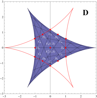
Figure 1. The intersection of the two deltoids is the fundamental region $\mathbb{D}$.

Let us denote the intersection of the two deltoids above by $\mathbb{D}:=\mathrm{ran}\varphi\cap\mathrm{ran}(-\varphi)$. It is clear that for any $\alpha\in\mathbb{D}$ one can define a complex Hadamard matrix in the following way: take any value of $\varphi^{-1}[\alpha]$, say $x,y$. Then we have $a=1,b=\overline{x},c=\overline{x}\overline{y}$. Similarly, take $\varphi^{-1}[-\alpha]$ to obtain the values of $u,v$. We have $d=1,e=\overline{u},f=\overline{u}\overline{v}$. In particular, we have

(11) $$X_{6}(\alpha)\equiv X_{6}(x,y,u,v)=\left[\begin{array}[]{cccccc}1&1&1&1&1&1\\ 1&x^{2}y&xy^{2}&\frac{xy}{uv}&uxy&vxy\\ 1&\frac{x}{y}&x^{2}y&\frac{x}{u}&\frac{x}{v}&uvx\\ 1&uvx&uxy&-1&-uxy&-uvx\\ 1&\frac{x}{u}&vxy&-\frac{x}{u}&-1&-vxy\\ 1&\frac{x}{v}&\frac{xy}{uv}&-\frac{xy}{uv}&-\frac{x}{v}&-1\end{array}\right].$$

In the rest of this section we describe an algebraic way of inverting $\varphi$, i.e. how we can determine $x,y$ and $u,v$ from a given $\alpha\in\mathbb{D}$. Considering the equation $\varphi[x,y]=\alpha$, we have

(12) $$x+y+\frac{1}{xy}=\alpha.$$

After conjugating and using the fact that $x,y,\in\mathbb{T}$ we have

(13) $$\frac{1}{x}+\frac{1}{y}+xy=\overline{\alpha}$$

Instead of solving the system of equations (12)–(13) we multiply equation (12) by $x^{2}\neq 0$ and (13) by $x\neq 0$ and rather consider their sum and difference respectively. In this way the variable $y$ vanishes from the difference and we obtain the following cubic equation for $x$, depending on $\alpha$.

(14) $$f_{\alpha}(x):=x^{3}-\alpha x^{2}+\overline{\alpha}x-1=0$$

It is important to realize that $y$ is a root of (14) by symmetry as well. Moreover, if $x$ and $y$ are distinct roots of (14) then (12) follows. For $\alpha\in\mathrm{int}\mathbb{D}$ the roots of (14) are distinct, and let us denote them by $r_{1},r_{2},r_{3}$. Our construction guarantees that two of them are unimodular. But as $r_{1}r_{2}r_{3}=1$ we conclude that the third root is unimodular as well. Hence one can choose $x$ as any of $r_{1},r_{2},r_{3}$, and choose $y$ as any other root. We therefore have $6$ choices for the ordered pair $(x,y)$.

Finally, let us substitute $-\alpha$ into (14), and denote the roots by $q_{1},q_{2},q_{3}$. The method to determine the values of $u,v$ is completely analogous to what we have presented for $x$ and $y$.

For $\alpha\in\mathrm{int}\mathbb{D}$ we therefore have $6\times 6=36$ choices for the ordered quadruple $(x,y,u,v)$. However an easy automatized calculation shows that all of the emerging matrices $X_{6}(x,y,u,v)$ are equivalent to one of the two matrices $X_{6}(r_{1},r_{2},q_{1},q_{2})$ or $X_{6}^{T}(r_{1},r_{2},q_{1},q_{2})$ (note that a complex Hadamard matrix is generically not equivalent to its transpose). On the boundary of $\mathbb{D}$, however, it is easy to show that the roots of (14) are $r,r$ and $\frac{1}{r^{2}}$ and the two families $X_{6}(r_{1},r_{2},q_{1},q_{2})$ and $X_{6}^{T}(r_{1},r_{2},q_{1},q_{2})$ are equivalent, and hence in this case all choices of the quadruple $(x,y,u,v)$ lead to equivalent matrices.

Finally we note that for every $\alpha\in\mathbb{D}$ $X_{6}(\alpha)$ is stable under conjugation, that is $X_{6}(r_{1},r_{2},q_{1},q_{2})$ and $\overline{X}_{6}(r_{1},r_{2},q_{1},q_{2})$ are equivalent.

By summarizing the contents of this section, we establish the main result of the paper.

Theorem 2.2.

There exist two previously unknown $2$-parameter non-affine families of complex Hadamard matrices of order $6$, $X_{6}(x,y,u,v)$ and $X_{6}^{T}(x,y,u,v)$, described by formula (11) and its transposed. For $\alpha\in\mathbb{D}$ the values of $x$ and $y$ are determined as roots of $f_{\alpha}$ in (14), while the values of $u$ and $v$ are determined as roots of $f_{-\alpha}$ in (14), respectively.

Proof.

The construction above lead us to a $2$-parameter family of complex Hadamard matrices as follows. For $\alpha\in\mathbb{D}$ let $r_{1}(\alpha),r_{2}(\alpha),r_{3}(\alpha)$ denote the roots of equation (14), being set as continuous functions of $\alpha$. For a given $\alpha\in\mathbb{D}$ one can set $x=r_{1}(\alpha)$ and $y=r_{2}(\alpha)$. Similarly, substitute $-\alpha$ into (14) and denote the roots as $q_{1}(\alpha),q_{2}(\alpha),q_{3}(\alpha)$, and set $u=q_{1}(\alpha)$ and $v=q_{2}(\alpha)$. Finally, define $X_{6}(\alpha)=X_{6}(x,y,u,v)$ as in formula (11). We emphasize again that easy permutation equivalences show that all choices of the roots $r_{i_{1}}(\alpha),r_{i_{2}}(\alpha),q_{i_{1}}(\alpha),q_{i_{2}}(\alpha)$ lead to matrices equivalent to $X_{6}(r_{1},r_{2},q_{1},q_{2})$ or $X_{6}^{T}(r_{1},r_{2},q_{1},q_{2}).$

The main claim of the Theorem is that this family (and its transposed) has not appeared in the literature so far. To show this, recall that with the exception of the Fourier families $F_{6}(a,b)$ and $F_{6}^{T}(a,b)$, all previously known families of order $6$ contain less than two parameters. Therefore we only need to exhibit one particular matrix from our family $X_{6}(\alpha)$ which does not belong to the Fourier families. Such a matrix can be obtained by choosing e.g. $\alpha_{0}=1$ on the boundary of $\mathbb{D}$. It is easy to show that in this case all choices of $(x,y,u,v)$ lead to a Hadamard matrix equivalent to $D_{6}$, which is not included in the families $F_{6}(a,b)$ and $F_{6}^{T}(a,b)$. Therefore, by continuity, in a small neighborhood $\mathcal{U}$ of $\alpha_{0}=1$ the family $X_{6}(\alpha)$ is disjoint from $F_{6}(a,b)$ and $F_{6}^{T}(a,b)$. Hence, inside this neighbourhood $\mathcal{U}$ only one-parameter curves can possibly produce already known complex Hadamard matrices of order 6, while generically $X_{6}(\alpha)$ is indeed new. ∎

This shows that the family $X_{6}(\alpha)$ is at least locally new, around $\alpha_{0}=1$. We expect that more is true: the family $X_{6}(\alpha)$ intersects the Fourier family only at $\alpha=0$.

3. Connections to previously discovered families

In this section we analyze how the obtained new family of complex Hadamard matrices $X_{6}$ is related to the previously discovered ones, such as $B_{6},D_{6},F_{6},M_{6}$ and $S_{6}$, respectively. In particular, we prove that both the Beauchamp–Nicoara family of self-adjoint complex Hadamard matrices and Diţă’s one-parameter affine family is contained in the orbit of $X_{6}(\alpha)$. Thus our construction in some sense unifies and extends some of the previously discovered families.

We shall denote the standard basis of $\mathbb{C}^{6}$ by $e_{i},i=1,2,\ldots,6$, which should be understood as column vectors. Also, for later purposes let us denote by $D[\alpha]$ the discriminant function associated to (14), i.e. let $r_{1},r_{2},r_{3}$ be the three roots of $f_{\alpha}$ and define

(15) $$D[\alpha]:=(r_{1}-r_{2})^{2}(r_{2}-r_{3})^{2}(r_{3}-r_{1})^{2}=|\alpha|^{4}+18|\alpha|^{2}-8\Re[\alpha^{3}]-27.$$

Clearly, $D[\alpha]\in\mathbb{R}$, and $\alpha\in\mathbb{D}$ if and only if $D[\alpha]\leq 0$ and $D[-\alpha]\leq 0$. Note also, that on the boundary of $\mathbb{D}$ we have $D[\alpha]=0$ or $D[-\alpha]=0$.

We begin our investigation with the center of $\mathbb{D}$, i.e. we consider the case $\alpha=0$. We have the following

Lemma 3.1.

For $\alpha=0$ one choice of $(x,y,u,v)$ in formula (11) leads to a Hadamard matrix equivalent to $F_{6}(1,3)$.

Proof.

Straightforward computation. ∎

Next we classify the “extremal” points of $\mathbb{D}$. It has six points which are farthest from the center, and another six which are closest to it. These points will be called “maximal”- and “minimal” extremal points of $\mathbb{D}$.

Lemma 3.2.

a) The six maximal extremal points of $\mathbb{D}$ can be obtained by choosing

(16) $$\alpha^{max}_{k}=\sqrt{-9+6\sqrt{3}}\mathbf{e}^{\mathbf{i}\left(\frac{\pi}{6}+k\frac{\pi}{3}\right)},k=1,2,\ldots,6$$

and lead to matrices equivalent to $C_{6}$.

b) The six minimal extremal points can be obtained by choosing

(17) $$\alpha^{min}_{k}=\mathbf{e}^{\mathbf{i}k\frac{\pi}{3}},k=1,2,\ldots,6$$

and lead to matrices equivalent to $D_{6}$.

Proof.

Straightforward computation. ∎

Somewhat surprisingly it turns out that the whole family $D_{6}(t)$ is included in in our family $X_{6}(\alpha)$. This was actually first found by Zauner [21]. We have the following

Proposition 3.3 (cf. Ex. 5.7. from [21]).

Let $D(t)$ be a complex Hadamard matrix of the form

(18) $$D(t)=\left[\begin{array}[]{cccccc}1&1&1&1&1&1\\ 1&-1&-\frac{\mathbf{i}}{t^{3}}&\mathbf{i}&-\mathbf{i}&\frac{\mathbf{i}}{t^{3}}\\ 1&-\mathbf{i}t^{3}&-1&-\mathbf{i}&\mathbf{i}t^{3}&\mathbf{i}\\ 1&\mathbf{i}&-\mathbf{i}&-1&\mathbf{i}&-\mathbf{i}\\ 1&-\mathbf{i}&\frac{\mathbf{i}}{t^{3}}&\mathbf{i}&-1&-\frac{\mathbf{i}}{t^{3}}\\ 1&\mathbf{i}t^{3}&\mathbf{i}&-\mathbf{i}&-\mathbf{i}t^{3}&-1\end{array}\right],$$

where $t\in\mathbb{T}$ is an indeterminate. Then $D(t)$ has a $2$-circulant representation.

Proof.

Let us define the unitary diagonal matrices $D_{1}=\mathrm{Diag}\left(1,\mathbf{i}t,\mathbf{i}/t,1,t,-1/t\right)$ and $D_{2}=\mathrm{Diag}\left(1,\mathbf{i}/t,\mathbf{i}t,1,1/t,-t\right)$. Then one gets

(19) $$D_{1}D(t)D_{2}=\left[\begin{array}[]{ccc|ccc}1&\frac{\mathbf{i}}{t}&\mathbf{i}t&1&\frac{1}{t}&-t\\ \mathbf{i}t&1&\frac{\mathbf{i}}{t}&-t&1&\frac{1}{t}\\ \frac{\mathbf{i}}{t}&\mathbf{i}t&1&\frac{1}{t}&-t&1\\ \hline\cr 1&-\frac{1}{t}&t&-1&\frac{\mathbf{i}}{t}&\mathbf{i}t\\ t&1&-\frac{1}{t}&\mathbf{i}t&-1&\frac{\mathbf{i}}{t}\\ -\frac{1}{t}&t&1&\frac{\mathbf{i}}{t}&\mathbf{i}t&-1\end{array}\right].$$

∎

Corollary 3.4.

All members of the Diţă-family $D_{6}(t)$ have a $2$-circulant representation.

Proof.

The family $D(t)$ above is trivially permutation equivalent to the Diţă-family $D_{6}(t^{3})$ as listed in [17]. ∎

Next we turn our attention to the family of self-adjoint complex Hadamard matrices.

Lemma 3.5.

On the boundary of $\mathbb{D}$ all emerging matrices are self-adjoint.

Proof.

Let us suppose that $\alpha\in\partial\mathbb{D}$. Then we have either $D[\alpha]=0$ or $D[-\alpha]=0$. Suppose that $D[\alpha]=0$. We have already seen that in this case the roots of (12) are $r,r$ and $\frac{1}{r^{2}}$, and as we obtain equivalent matrices we are free to set $x=r$, $y=\frac{1}{r^{2}}$. Then, as we have $b=\overline{x}$, $c=\overline{x}\overline{y}$, the statement follows from Remark 2.1. The case $D[-\alpha]=0$ is completely analogous. ∎

It turns out that all complex self-adjoint Hadamard matrices of order 6 have a 2-circulant representations.

Proposition 3.6.

Let $B$ be a complex Hadamard matrix of the form

(20) $$B=\left[\begin{array}[]{cccccc}1&1&1&1&1&1\\ 1&-1&-\frac{1}{x}&-y&y&\frac{1}{x}\\ 1&-x&1&y&\frac{1}{z}&-\frac{1}{xyz}\\ 1&-\frac{1}{y}&\frac{1}{y}&-1&-\frac{1}{xyz}&\frac{1}{xyz}\\ 1&\frac{1}{y}&z&-xyz&1&-\frac{1}{x}\\ 1&x&-xyz&xyz&-x&-1\end{array}\right].$$

Then $B$ has a $2$-circulant representation.

Proof.

Let us define permutational matrices $P=\left[e_{1},e_{4},e_{2},e_{5},e_{3},e_{6}\right],Q=\left[e_{5},e_{1},e_{3},e_{4},e_{6},e_{2}\right]$, and the following unitary diagonal matrices $D_{1}=\mathrm{Diag}\left(1,\sqrt[3]{z},1/\sqrt[3]{z},1/y,\sqrt[3]{z},-1/(xy\sqrt[3]{z})\right)$ and $D_{2}=\mathrm{Diag}\left(1,1/\sqrt[3]{z},1/z^{2/3},1,-xyz^{2/3},y\sqrt[3]{z}\right)$. Here, $\sqrt[3]{z}$ denotes the principal cubic root of $z$, and $z^{2/3}$ is the (slightly abusive) notation of $\left(\sqrt[3]{z}\right)^{2}$. Now we see that $D_{1}PBQD_{2}$ is $2$-circulant, in particular

(21) $$D_{1}PBQD_{2}=\left[\begin{array}[]{ccc|ccc}1&\frac{1}{\sqrt[3]{z}}&\frac{1}{z^{2/3}}&1&-xyz^{2/3}&y\sqrt[3]{z}\\ \frac{1}{z^{2/3}}&1&\frac{1}{\sqrt[3]{z}}&y\sqrt[3]{z}&1&-xyz^{2/3}\\ \frac{1}{\sqrt[3]{z}}&\frac{1}{z^{2/3}}&1&-xyz^{2/3}&y\sqrt[3]{z}&1\\ \hline\cr 1&\frac{1}{y\sqrt[3]{z}}&-\frac{1}{xyz^{2/3}}&-1&-z^{2/3}&-\sqrt[3]{z}\\ -\frac{1}{xyz^{2/3}}&1&\frac{1}{y\sqrt[3]{z}}&-\sqrt[3]{z}&-1&-z^{2/3}\\ \frac{1}{y\sqrt[3]{z}}&-\frac{1}{xyz^{2/3}}&1&-z^{2/3}&-\sqrt[3]{z}&-1\end{array}\right].$$

∎

As the elegant characterization of Beauchamp and Nicoara [1] shows, all self-adjoint Hadamard matrices of order $6$ are equivalent to a matrix described by (20).

Corollary 3.7.

All self-adjoint Hadamards of order $6$ has the $2$-circulant representation.

We close this section with the following remark: matrices $M_{6}$ and $S_{6}$ are not members of the family $X_{6}(\alpha)$. It was explicitly stated in [11], that $M_{6}$ and $\overline{M}_{6}$ are inequivalent, and hence a local neighborhood around the one-parametric matrix $M_{6}$ avoids the family $X_{6}$, which is stable under conjugation. Clearly, as $S_{6}$ is isolated, it cannot be a member of a continuous family of matrices.

4. The existence of a two-parameter family of MUB-triplets in $\mathbb{C}^{6}$

Recall that a family of mutually unbiased bases (MUBs) $\{\mathcal{B}_{1},\mathcal{B}_{2},\ldots,\mathcal{B}_{k}\}$ is a collection of orthonormal bases of $\mathbb{C}^{n}$ such that $\left|\left\langle e,f\right\rangle\right|=1/\sqrt{n}$ whenever $e\in B_{i}$ and $f\in B_{j}$ for some $i\neq j$. One can assume that $\mathcal{B}_{1}$ is the standard basis, and hence the coordinates of the vectors of all the remaining bases have modulus $1/\sqrt{n}$. In particular, the column vectors of the remaining bases — up to a constant factor — form complex Hadamard matrices. It is well known that at most $n+1$ MUBs can be constructed, and this upper bound is sharp whenever $n$ is a prime power. On the other hand, when $n$ is composite, not much is known about the existence of mutually unbiased bases. For a quick introduction to MUBs we refer the reader to [2], [20]. In this section the existence of a two-parameter family of MUB-triplets of order $6$ is concluded. The method described here was discovered by Zauner [21], who exhibited a one-parameter family of triplets earlier. Interestingly, the heart of his construction was the existence of the infinite family of $2$-circulant complex Hadamard matrices described by formula (19), which he used as a seed matrix for producing MUB triplets. We recall his machinery and apply it to the two-parameter matrix $X_{6}(\alpha)$. First we recall a simple, but extremely useful lemma on the representation of $2\times 2$ unitaries.

Lemma 4.1 (cf. Lemma 5.5. from [21]).

Suppose that $M$ is a $2\times 2$ unitary matrix with entries $a,b,c$ and $d$. Then there exists $u,v,x,y\in\mathbb{T}$, such that

(22) $$M=\left[\begin{array}[]{cc}a&b\\ c&d\\ \end{array}\right]=\frac{1}{2}\left[\begin{array}[]{rr}u+v&y\left(u-v\right)\\ \frac{\left(u-v\right)}{x}&\frac{y\left(u+v\right)}{x}\\ \end{array}\right].$$

$\hfill\square$

Before proceeding we need to introduce some notations. Let $T$ be a $2m\times 2m$ block matrix with $m\times m$ blocks as the following:

(23) $$T=\left[\begin{array}[]{cc}A&B\\ C&D\\ \end{array}\right].$$

Further let $U,V,X,Y$ are arbitrary unitary diagonal matrices, and let us define the following matrices with the aid of the Fourier matrix $F_{m}$ as

(24) $$Z_{1}=\frac{1}{\sqrt{2}}\left[\begin{array}[]{rr}F_{m}&XF_{m}\\ F_{m}&-XF_{m}\\ \end{array}\right],Z_{2}=\frac{1}{\sqrt{2}}\left[\begin{array}[]{rr}UF_{m}&UYF_{m}\\ VF_{m}&-VYF_{m}\\ \end{array}\right].$$

Note that as $F_{m}$ is unitary, so are $Z_{1},Z_{2}$ and hence also

(25) $$Z_{1}^{-1}Z_{2}=\frac{1}{2}\left[\begin{array}[]{cc}F_{m}^{-1}\left(U+V\right)F_{m}&F_{m}^{-1}\left(\left(U-V\right)Y\right)F_{m}\\ F_{m}^{-1}\left(X^{-1}\left(U-V\right)\right)F_{m}&F_{m}^{-1}\left(X^{-1}Y\left(U+V\right)\right)F_{m}\\ \end{array}\right].$$

In [21] Zauner characterized $2$-circulant unitary matrices in the following way. We quote his result with a sketched proof for completeness.

Proposition 4.2 (cf. Prop. 5.6. from [21]).

$T$ is a $2$-circulant unitary matrix with blocks $A,B,C,D$ if and only if there exist $2m\times 2m$ (rescaled) complex Hadamard matrices $Z_{1},Z_{2}$ as in formula (24), such that $T=Z_{1}^{-1}Z_{2}$.

Proof (Sketch).

Suppose that $Z_{1},Z_{2}$ are given as above. Clearly $Z_{1}^{-1}Z_{2}$ is unitary. Also, for every diagonal matrix $D$ the matrix $F_{m}^{-1}DF_{m}$ is circulant, and hence $T$ is a $2$-circulant unitary by formula (25).

For the converse, suppose that $T$ is an arbitrary $2$-circulant unitary matrix. Then one can write $T$ as

(26) $$T=\left[\begin{array}[]{cc}F_{m}^{-1}&0\\ 0&F_{m}^{-1}\\ \end{array}\right]\left[\begin{array}[]{rr}\tilde{A}&\tilde{B}\\ \tilde{C}&\tilde{D}\\ \end{array}\right]\left[\begin{array}[]{cc}F_{m}&0\\ 0&F_{m}\\ \end{array}\right],$$

with diagonal matrices $\tilde{A},\tilde{B},\tilde{C},\tilde{D}$. It follows that $T$ is unitary if and only if the matrices

(27) $$S_{k}=\left[\begin{array}[]{rr}a_{k}&b_{k}\\ c_{k}&d_{k}\\ \end{array}\right]$$

are unitary for every $1\leq k\leq m$. Now use Lemma 4.1 to represent $S_{k}$ with unimodular elements $u_{k},v_{k},x_{k},y_{k}$, from which one readily defines the unitary diagonal matrices $U,V,X,Y$, and finally $Z_{1}$ and $Z_{2}$ through formula (24). We conclude by observing that in this setting formulas (25) and (26) coincide. ∎

Proposition 4.2 describes how to construct a triplet of MUBs from a given $2$-circulant complex Hadamard matrix $T$. Clearly, the assumption that $T=Z_{1}^{-1}Z_{2}=Z_{1}^{\ast}Z_{2}$ is a complex Hadamard matrix implies that $\{I,Z_{1},Z_{2}\}$ is a collection of $3$ MUBs of order $2m$. Note, however, that in order to use this construction one needs to begin with a suitable complex Hadamard matrix $T$ first, from which the unbiased bases $Z_{1}$ and $Z_{2}$ can be constructed. Clearly, the newly discovered matrix $X_{6}(\alpha)$ is a perfect seed matrix for Zauner’s construction. In summary, we have proved the following

Theorem 4.3.

There exists a two-parameter family of MUB-triplets of order $6$ emerging from the family $X_{6}(\alpha)$ via Zauner’s construction described in Proposition 4.2.

We conclude our paper by the following observation: it is plausible that our new family $X_{6}(\alpha)$ intersects the Fourier families only at $\alpha=0$. If one could exhibit similar families $X_{6}^{{a,b}}(\alpha)$ for all members $F(a,b)$ of the Fourier families, that would provide a rigorous proof of the existence of a 4-parameter family of complex Hadamard matrices of order $6$. The existence of such a family is strongly indicated by the numerical results of [15]. This could possibly lead to a full classification of complex Hadamard matrices of order $6$.

References

- [1] K. Beauchamp, R. Nicoara: Orthogonal maximal Abelian -subalgebras of the matrices, Linear Algebra Appl. 428, No. 8-9, 1833–1853 (2008).
- [2] I. Bengtsson, W. Bruzda, Å. Ericsson, J. Larsson, W. Tadej, K. Życzkowski: MUBs and Hadamards of order , J. Math. Phys. 48, 052106 (2007)
- [3] G. Björck: Functions of modulus on , whose Fourier transform have constant modulus, and “cyclic -roots”. Recent Advances in Fourier Analysis and its applications. NATO Adv. Sci. Int. Ser. C: Math. Phys. Sci., Kluwer 315., 131–140. (1990)
- [4] P. Diţă: Some results on the parametrization of complex Hadamard matrices, J. Phys. A, 37 no. 20, 5355–5374. (2004)
- [5] U. Haagerup: Orthogonal maximal Abelian -subalgebras of matrices and cyclic -roots, Operator Algebras and Quantum Field Theory (Rome), Cambridge, MA International Press, (1996), 296–322.
- [6] P. de la Harpe, V. F. R. Jones: Paires de sous-algebres semi-simples et graphes fortement reguliers, C.A. Acad. Sci. Paris, 311, serie I (1990), 147–150.
- [7] K. J. Horadam: Hadamard Matrices and Their Applications, Princeton University Press (2007)
- [8] P. Jaming, M. Matolcsi, P. Móra, F. Szöllősi, M. Weiner: An Infinite Family of MUB-triplets in dimension . arXiv:0902.0882v1 [quant-ph]
- [9] M. Kolountzakis, M. Matolcsi: Tiles with no spectra, Forum math, 18, (2006), 519–528.
- [10] M. Matolcsi, J. Réffy, F. Szöllősi: Constructions of complex Hadamard matrices via tiling Abelian groups, Open Syst. Inf. Dyn., 14:3, 247–263. (2007)
- [11] M. Matolcsi, F. Szöllősi: Towards the classification of complex Hadamard matrices, Open Sys. & Inf. Dyn. 15:2, 93–108. (2008)
- [12] A. Munemasa, Y. Watatani: Orthogonal pairs of -subalgebras and association schemes, C.R. Acad. Sci. Paris, 314, serie I (1992), 329–331.
- [13] M. Petrescu: Existence of continuous families of complex Hadamard matrices of certain prime dimensions, PhD thesis, UCLA (1997)
- [14] S. Popa: Orthogonal pairs of -subalgebras in finite von Neumann algebras, J. Operator Theory, 9, 253-268 (1983).
- [15] A. J. Skinner, V. A. Newell, R. Sanchez: Unbiased bases (Hadamards) for 6-level systems: Four ways from Fourier preprint: arXiv:0810.1761v1 [quant-ph]
- [16] F. Szöllősi: Parametrizing Complex Hadamard Matrices, European Journal of Combinatorics 29, 1219–1234. (2008)
- [17] W. Tadej, K. Życzkowski: A concise guide to complex Hadamard matrices, Open Syst. Inf. Dyn. 13, 133-177. (2006)
- [18] T. Tao: Fuglede’s Conjecture Is False in and Higher Dimensions. Math Res. Letters, 11, 251–258. (2004)
- [19] Website for complex Hadamard matrices: http://chaos.if.uj.edu.pl/karol/hadamard/
- [20] R. F. Werner: All teleportation and dense coding schemes, J. Phys. A, 34, (2001), 7081–7094.
- [21] G. Zauner: Orthogonale Lateinische Quadrate und Anordnungen, Verallgemeinerte Hadamard-matrizen und Unabhängigkelt in der Quanten-Wahrscheinlichkeitestheorie, Master Thesis, Universität Wien (1991)