CMBPol Mission Concept Study
Reionization Science with the Cosmic Microwave Background
Matias Zaldarriaga1,2, Loris Colombo3, Eiichiro Komatsu4, Adam Lidz1, Michael Mortonson5, S. Peng Oh6, Elena Pierpaoli3, Licia Verde7,8, Oliver Zahn9,10
Abstract
We summarize existing constraints on the epoch of reionization and discuss the observational probes that are sensitive to the process. We focus on the role large scale polarization can play. Polarization probes the integrated optical depth across the entire epoch of reionization. Future missions such as Planck and CMBPol will greatly enhance our knowledge of the reionization history, allowing us to measure the time evolution of the ionization fraction. As large scale polarization probes high redshift activity, it can best constrain models where the Universe was fully or partially ionized at early times. In fact, large scale polarization could be our only probe of the highest redshifts.
1 Center for Astrophysics, Harvard University, Cambridge, MA 02138, USA
2 Department of Physics, Harvard University, Cambridge, MA 02138, USA
3 Department of Physics and Astronomy, University of Southern California, Los Angeles, CA 90089, USA
4 Department of Astronomy, The University of Texas at Austin, Austin, TX 78712, USA
5 Department of Physics, University of Chicago, Chicago, IL 60637, USA
6 Department of Physics, University of California, Santa Barbara, CA 93106, USA
7 ICREA & Institute of Space Sciences (CSIC-IEEC), Campus UAB, Bellaterra, Spain
8 Department of Astrophysical Sciences, Princeton, NJ 08540, USA
9 Berkeley Center for Cosmological Physics, University of California, Berkeley, Berkeley, CA 94720, USA
10 Lawrence Berkeley National Laboratory, Berkeley, CA 94720, USA
1 The Epoch of Reionization: How the Universe emerges from its dark ages
1.1 Introduction
Perhaps the most important goal of observational cosmology is to understand how structure arose in our Universe, how the stars, galaxies, and quasars around us today and at high redshifts formed. We currently believe that small density perturbations were imprinted onto the Universe during the inflationary era which then grew through gravitational instability, producing halos as well as the cosmic web of sheets and filaments. Measurements of the cosmic microwave background (CMB) anisotropies have been instrumental in establishing this picture (e.g. [1]).
To understand the CMB measurements or the large scale clustering properties of galaxies one only needs to understand the structure formation process in the linear regime. However, in order to understand how baryons collapsed into bound objects such as galaxies and galaxy clusters, and to determine how these objects affect their surroundings we need to take structure formation beyond the well-understood linear regime. At low or moderate redshifts (), galaxies and quasars can be observed directly with existing technology. However, the first generations of protogalaxies are not yet similarly accessible and the full population of galaxies and quasars at intermediate redshifts () remains unknown.
One approach to investigating the properties of galaxies and quasars is through their impact on the intergalactic medium (IGM). In particular, it is believed that radiation from these objects reionized the IGM and that this process depends on the distribution and nature of the ionizing sources. Thus, an understanding of reionization coupled with detailed measurements has the potential to significantly constrain models for the formation and evolution of galaxies and quasars.
Observational evidence indicates that the IGM was reionized in two distinct phases. The first phase, completed by , led to the ionization of hydrogen as well as singly ionizing helium. However, the early sources of ionizing radiation would not have been energetic enough to doubly ionize helium (if they were stellar). The second phase of the reionization of the IGM, corresponding to the conversion of HeII into HeIII, thus likely occurred later, when a sufficient population of hard sources (i.e. quasars) developed, and observations indicate that this happened at .
Reionization encodes a wealth of information about the ionizing sources. For example, in the case of hydrogen reionization, the first sources of radiation likely formed in overdense regions, ionizing pockets of nearby gas. As more sources formed these regions grew and eventually overlapped. Because the structure of these regions and their growth depend on the nature, clustering, and abundance of the sources, the timing, morphology, and duration of reionization are highly sensitive to the properties of the first luminous objects and their relationship to the IGM (e.g., [2, 3, 4, 5, 6, 7, 8, 9, 10]).
Empirical studies of the reionization of hydrogen (sometimes referred to as the Epoch of Reionization [EoR]) have placed constraints on this event but have not yet mapped it in detail. One constraint comes from the effects of the ionized gas on the CMB. The free electrons Thomson scatter CMB photons, washing out the intrinsic anisotropies but generating a polarization signal on large angular scales. The total scattering optical depth is proportional to the column density of ionized hydrogen, so it provides an integral constraint on the reionization history. Recently, the Wilkinson Microwave Anisotropy Probe111See http://map.gsfc.nasa.gov/. (WMAP) collaboration used five years worth of data to improve their determination of [1]. The combined analysis of WMAP and large scale structure data such as that coming from the Sloan Digital Sky Survey222See http://www.sdss.org/. (SDSS) indicates that reionization probably happened in the redshift range . More detailed information on the reionization history could be obtained by precisely measuring the large angular scale polarization [11, 12, 13]. It is the goal of this white paper to discuss this possibility further.
Along with the large scale CMB polarization measurements, we anticipate a wealth of other upcoming observations that will increase our knowledge of the EoR. The EoR and the preceding ‘dark ages’ – i.e., the period after cosmological recombination but before the birth of the first luminous sources – are the only remaining phases of structure formation as yet to be directly observed. As such, the study of the EoR is a research frontier for both observational and theoretical cosmology, and will grow as an increasingly active and exciting research field in upcoming years. We describe current constraints and future prospects from other observations in §2, and consider the way in which large scale CMB polarization measurements may complement these observations throughout this white paper.
1.2 Motivating questions and how to answer them
We believe that the study of reionization will shed light on the early process of structure formation. In practice we want to answer several specific questions about this early time in the history of our Universe. We want to determine which sources were responsible for reionization. Were they a population of early galaxies similar to present day ones? Were Population III stars important for this process? Did quasars or mini-quasars play a role? Did the sources of ionizing radiation sit in high or low mass galaxies? Did the ionizing radiation produced by the first sources have a strong feedback effect on the galaxy formation process, drastically changing the way galaxy formation proceeded thereafter?
In some sense the study of reionization is akin to using the IGM as a laboratory for learning about the first sources and the earliest stages of the structure formation process. In order to understand how the study of the IGM can help us answer these questions, it is useful to think of two separate characterizations of the process. First we can think of the evolution of the average ionization fraction of hydrogen with time and we can subsequently consider the spatial fluctuations around that mean evolution. The latter is the study of the sizes of the ionized bubbles and the morphology of the ionized regions. This split is useful because different observational probes have different sensitivities to these different aspects. Furthermore the study of the mean and the spatial fluctuations are sensitive to different properties of the first sources.
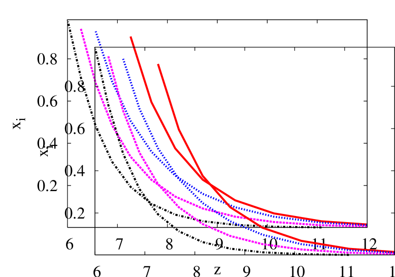
To learn about what type of halos the sources lived in one can study how rapid the evolution of the mean ionization fraction is. Sources that live in rarer more massive halos usually lead to a faster evolution of the mean. The time and duration of reionization also depends on the clumpiness of the IGM, as well as on radiative, chemical, and mechanical feedback from the first sources, which impact the formation of sources forming later on. An example of the type of information contained in the redshift evolution of the mean ionization fraction is shown in Figure 1, which demonstrates the impact of radiative feedback.
Furthermore any evidence of ionized hydrogen at very early times could signal the existence of an early and very efficient mode of star formation or perhaps an entirely new source of ionizing photons such as those that could come from annihilating or decaying dark matter. The study of large scale CMB polarization is probably the best and only probe of these very early stages of the ionization history and thus it is probably the only way to constrain some of these scenarios.
The study of the spatial variations of the ionization fraction during reionization, that is determining the size distribution of the ionized regions, also encodes a wealth of information about the sources responsible for reionization. A simulated model, illustrating spatial variations in the ionization fraction, is shown in Figure 2. The size distribution is mainly dependent on the clustering properties of the sources which in turn can help determine what mass halos those sources typically inhabit. Furthermore, and especially during the later stages of reionization, the presence of high density regions that act as photon sinks can set a maximum size for the ionized bubbles. Thus there is the potential to learn about the small scale density structure of the IGM.
1.3 Outline of this White Paper
In section 2 we will describe different probes that can be used to constrain the ionization history of the universe. In section 3 we focus on the information that can be extracted from the large scale polarization of the CMB. In section 4 we comment on the impact uncertainties in the ionization history have on the determination of other cosmological parameters. Finally for completeness in section 5 we discuss the measurement of secondary anisotropies.
2 Survey of observational probes
As mentioned in the introduction, a confluence of data sets from a variety of different observational probes should soon provide significant advances in our understanding of the EoR. In order to best understand how CMBPol may help with the study of reionization, we briefly describe several future probes, examining in particular how large scale polarization measurements may complement constraints from these other exciting studies. As we will see, upcoming observations should provide detailed constraints on reionization activity at redshifts close to and a bit higher than while large scale polarization, and CMBPol in particular, may be our best way to study reionization at higher redshifts, , in the near future.
We describe here four current and upcoming probes of reionization: high redshift quasar spectra, surveys for Ly- emitting galaxies, optical afterglow spectra of gamma-ray bursts, and 21 cm observations of the high redshift IGM. In §5 we additionally discuss constraints from small scale CMB measurements, which will be made by several upcoming experiments, and potentially by CMBPol, provided its angular resolution is high enough. We also discuss the related topic of metal absorption.
2.1 High Redshift Quasar Spectra
Presently, our most detailed probe of the high redshift () IGM comes from Ly- forest absorption spectra towards high redshift quasars. Regions with relatively large densities should appear as absorption troughs in quasar spectra, which presumably deepen and come to dominate as we approach the reionization epoch. Indeed, spectra of quasars selected from the SDSS show some extended regions of zero transmission [16]. Unfortunately, the Ly- cross section is very large and a relatively low average neutral fraction at the level of is sufficient to give complete absorption in the Ly- forest [17]. This makes it difficult to distinguish a largely neutral IGM from a significantly ionized one with this probe.
Nevertheless, several detailed studies have examined whether these spectra may indeed probe the IGM before reionization completes. These analyses have considered a range of different statistics: the redshift evolution of the average absorption in the Ly- and Ly- forest, the amount of scatter in the absorption from sightline to sightline, the abundance and extent of dark gaps in the high redshift Ly- forest, the properties of the proximity zone regions in high redshift quasar spectra, the redshift evolution of metal abundances, and the temperature of the IGM from the Ly- forest.
A plot of the redshift evolution of the Ly- opacity is shown in Figure 3. More precisely, we show the redshift evolution of the effective Ly- opacity, defined by , where is the average flux transmitted through the Ly- forest. One can see that the opacity at is typically very large, , with some sightlines having only lower limits on the opacity – i.e., they are consistent with complete absorption in the Ly- forest. As mentioned before, complete absorption in the Ly- forest at only implies a weak constraint on the average neutral fraction. A slightly stronger constraint comes from spectra with complete absorption in the Ly- region of the forest. Since the Ly- cross section is a factor of times smaller than that for Ly- absorption, complete Ly- absorption implies a more stringent lower limit on the neutral fraction than complete absorption in Ly-, but the resulting constraints are still consistent with a mostly ionized IGM [17].
A second feature of this figure, however, is that the opacity appears to evolve rather sharply with redshift around . Perhaps the sharp evolution in the opacity is signaling correspondingly rapid changes in the ionization state of the IGM? This is currently a matter of debate. In [17] the authors fit a power-law to data (shown as the black dashed line in Figure 3), and find that the data show a rapid upward departure from this fit [17]. Using a simulated model for the IGM density distribution [20], they argue that this upward departure requires very rapid evolution in the ionization state of the IGM. On the other hand, the authors of [19] use an empirically motivated fit to the opacity distribution and claim that rapid changes in the ionization state are not required [19]. The blue solid line in Figure 3 shows an extrapolation of their model from data to higher redshift, assuming a slowly varying ionization state. This model also fits the Ly- opacity data. The main issue here is that, even in a highly ionized IGM, the Ly- absorption cross section is so large that only quite underdense regions allow transmission through the Ly- forest. This means that the opacity evolution is sensitive to the precise abundance of underdense regions, as are the constraints on the ionization state ([21], [22]). Further theoretical modeling may help resolve this debate.
In addition to the large average absorption, the scatter in the absorption from sightline to sightline is quite large at [17]. Indeed, the colored points in Figure 3 show order unity variations in the opacity, after averaging over or co-moving Mpc/. These variations might indicate incomplete and patchy reionization with some sightlines piercing through mostly ionized gas, and others passing through long neutral stretches [23]. However, variations in the line of sight density field give rise to surprisingly large opacity fluctuations at , and so it is difficult to discern, on the basis of this scatter, whether these spectra really probe the IGM before reionization completes [22]. Current measurements appear at least broadly consistent with density fluctuations alone [22, 24].
The tightest constraints claimed on the ionization state of the IGM come from measurements of the proximity regions around quasars. Several authors, starting with [25], have argued that these regions are small, indicating that quasar ionization fronts are expanding into a largely neutral IGM [25, 26, 27]. However, subsequent more detailed studies have shown that it is hard to distinguish the case of a quasar ionization front expanding into a partly neutral IGM, and the case of a mere proximity zone in a mostly ionized IGM (e.g., [28, 29]). Detailed modeling of inhomogeneous reionization, incorporating the tendency for quasars to live in overdense regions that are ionized before typical regions, is required to best interpret these observations [29].
One can also measure the redshift evolution of metal line abundances in high redshift quasar spectra, and use this to constrain the reionization history. The mass density in Carbon IV appears to be a surprisingly flat function of redshift from [30, 31], requiring significant levels of star formation and metal enrichment prior to . Another metal line tracer is the OI line which has an ionization potential similar to that of hydrogen, lies redward of Ly-, and has a significantly lower optical depth than Ly-, making it a potential probe of the IGM before reionization completes [32]. In fact, high-resolution Keck spectra of the SDSS quasars do reveal some OI lines, with out of detected systems lying towards the highest redshift quasar presently known [33]. Interestingly, some of the OI systems are nearby regions that show transmission in the Ly- and Ly- forests of this quasar [33]. The interpretation of these observations is unclear: the OI systems might reflect dense clumps of neutral gas in a highly ionized IGM, or instead could indicate inhomogeneous metal pollution in a more neutral IGM.
A final constraint comes from measurements of the temperature of the Lyman- forest at –, which suggest an order unity change in the ionized fraction at [34, 35], although this argument depends on the timing and history of reionization (e.g., [36, 37]).
Some progress will be made in the near future by detecting more quasars, some at higher redshifts (), using widefield, deep near-IR surveys, although the rarity of bright background quasars at these redshifts makes this challenging. Improvements in modeling inhomogeneous reionization should also help our understanding of absorption spectra [38, 29, 39]. However, the large Ly- opacity expected in a mostly ionized medium is clearly a fundamental limitation, and it is likely impossible to study all but the final stages of reionization with this approach.
2.2 Lyman-alpha Emitters
An effective way to find high redshift galaxies is to search for their Ly- emission lines, since young galaxies frequently have strong Ly- emission [40]. Ly- emission searches have an advantage over high redshift Lyman break surveys in that they target narrow wavelength intervals, in between strong night sky background lines, in search of prominent emission lines. This allows one to detect galaxies that are unobservable by Lyman break selection owing to the strong night sky background at relevant wavelengths. Existing surveys have discovered several hundred galaxies with this technique (e.g., [41, 42, 43, 44, 45, 46, 47, 48, 49]), and other programs will begin taking data soon (e.g., [50, 51, 52]). The largest existing high redshift sample from the Subaru Deep Field consists of approximately galaxies above [46].
During the EoR, neutral hydrogen gas in the IGM will extinguish galactic Ly- emission lines. Specifically, the optical depth to Ly- absorption in a significantly neutral IGM is so large that even the red side of the Ly- line is attenuated by damping wing absorption [54]. As a result, galaxies that lie sufficiently close to the edge of an HII region, next to a significant column of neutral hydrogen, will be unobservable in Ly-. On the other hand, galaxies which reside towards the center of a sufficiently large HII region avoid complete attenuation, and will still be visible in Ly- emission. Since large HII regions form around high density peaks, one expects the clustering of Ly- emitters to increase dramatically towards the start of reionization [55, 53, 56]. In conjunction, the abundance of Ly- emitters should drop off rapidly as one looks back deeper into the EoR.
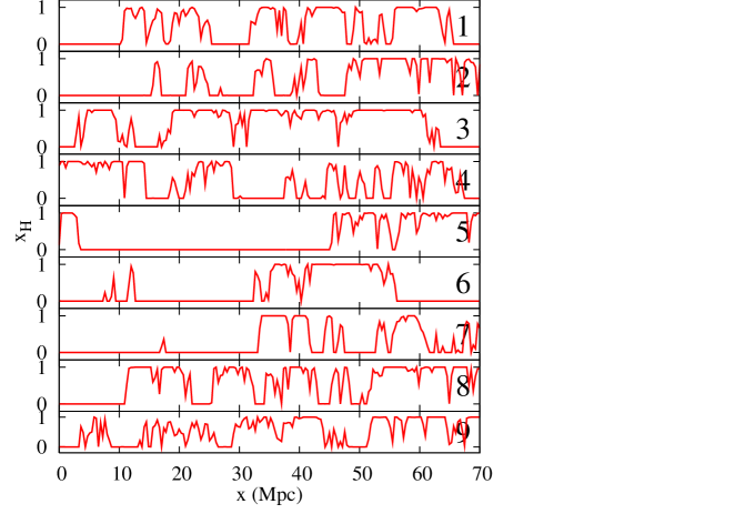
These trends can be seen in the simulation slices of Figure 4. Comparing the top, middle, and bottom panels, one can see how the presence of ionized bubbles modulates the abundance of emitters observable in Ly-: sources close to the center of large ionized regions are observable, while other sources are attenuated out of the Ly- sample. Comparing the left-most and right-most panel, it is clear that the suppression is much more significant in the earliest stages (here when the volume ionized fraction is ), compared to later stages (here when ). It is also clear that – since the ionized regions quickly grow rather large – one needs to observe a large field of view to reliably measure the abundance and clustering of Ly- emitters during reionization. To best constrain reionization with this technique, one hence wants a widefield survey that is deep enough to find large samples of emitters in the early stages of reionization.
Several authors have, in fact, used existing Ly- emitter samples to place constraints on the ionization state of the IGM. Malhotra & Rhoads [57] constrained the ionized volume fraction in the IGM by counting the abundance of Ly- emitters at , and requiring a minimum ionized volume around the sources to avoid attenuating their Ly- photons. From this argument, they find that more than of the volume of the IGM is ionized at . Kashikawa et al. [46] observe a decline in the bright end of the luminosity function between and , which they attribute to incomplete reionization at . Several other authors argue, however, that the observed evolution is consistent with evolution in a post-reionization IGM [14, 58, 59]. Finally, McQuinn et al. [53] use the clustering of the Subaru Deep Field sample to exclude a significantly neutral Universe with at confidence.
Further progress can be expected, with numerous planned surveys attempting to find Ly- emitters at high redshift. In particular, an extension to the existing Subaru Deep Field survey should extend measurements to over a deg2 field of view. This amounts to a factor of boost in field of view compared to the existing Subaru Deep Field. It will likely be difficult to push this method to significantly higher redshifts, since strong night sky emission lines force one to make near IR measurements from space, and since we require observations over a wide field of view. We expect this method to be most interesting in the near future if a significant fraction of the volume of the IGM is still neutral near .
2.3 GRB Optical Afterglows
Another possibility is to search for damping wing absorption in high redshift GRB optical afterglow spectra [54, 60, 61, 62]. These sources are extremely luminous, can potentially be detected at very high redshift, and have the important advantage of a simple power-law intrinsic spectrum. Additionally, GRBs are more likely to exist in typical HII regions than quasars or the massive, highly luminous galaxies that are easiest to detect at high redshift. Thus it may be possible to identify damping wing absorption in individual GRB afterglow spectra.
A difficulty with this probe of reionization, however, is that many optical afterglows show damped Ly- absorption from neutral hydrogen in the GRB host galaxy, at a level that is large enough to overwhelm the damping wing opacity from neutral gas in the surrounding IGM. For example, the highest redshift GRB afterglow detected thus far, at [61], shows evidence for a strong Damped Ly- Absorber (DLA) in its host, with a column density of . This absorption (shown in Figure 5) is so strong that it is difficult to tell whether or not there is damping wing absorption from the surrounding IGM. The damping wing profile from extended neutral gas in the IGM has a different wavelength dependence than that from a compact, local absorber, and we can therefore still hope to unambiguously detect neutral gas in the IGM using GRB afterglow spectra [54]. To detect the IGM damping wing, a GRB with a weaker local absorber, smaller than roughly , is needed. In addition, a high signal-to-noise spectrum is desirable, demanding rapid near IR follow-up of probable high redshift bursts. Some afterglow spectra at lower redshift show local absorbers with significantly smaller column density than the burst, and occasional spectra show no DLAs whatsoever [63]. We may therefore hope to find a clean line of sight towards a GRB at higher redshift and apply this test.
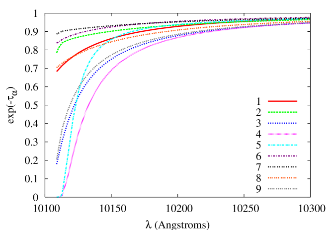
While GRB optical afterglow spectra may provide a good way of detecting the presence of neutral hydrogen in the IGM, perhaps even at very high redshift, it will be difficult to extract the ionized fraction from such measurements. The challenge here is that reionization is expected to be extremely inhomogeneous and the level of damping wing absorption should vary considerably towards one GRB host or another. Some GRBs will reside in large HII regions even rather early in the reionization process, since large ionized regions can form under the collective influence of highly clustered neighboring galaxies. The GRBs in large HII regions will suffer little damping wing absorption, while GRBs in smaller ionized bubbles or close to the edge of a large bubble will suffer more damping wing absorption [62]. This is illustrated in Figure 6, which shows that even when the IGM is as much as half neutral, there will be significant scatter in the level of damping wing absorption. This is similar to the effect depicted in Figure 4, but here we are attempting to extract information based on the spectrum of an individual object, rather than statistical trends based on the abundance and clustering of an entire population of galaxies. Extracting the ionized fraction from this method may require a prohibitively large sample of high redshift afterglows. We are hopeful that this method will definitively detect neutral gas at high redshift, indicating that reionization is not yet complete at a given redshift, but expect other probes to best map out the redshift evolution of the ionized fraction.
2.4 The 21 cm Line
One of the best ways to study reionization may be to detect redshifted 21 cm emission from neutral hydrogen gas in the high redshift IGM. Whenever the spin temperature of neutral hydrogen is different from the CMB temperature, neutral hydrogen atoms can be seen either in emission or absorption against the CMB at the redshifted wavelength of their 21 cm transition. After the first sources appear, the gas is expected to have been heated and the kinetic temperature of the gas should exceed that of the CMB [64]. Furthermore, Ly- photons from the first sources should couple the spin temperature of the 21 cm transition to the gas temperature long before the IGM is significantly ionized [65]. Thus, hydrogen should appear in emission during the EoR and high resolution observations of the 21 cm transition as a function of both frequency and angle can provide a three-dimensional map of reionization (e.g., [66, 67]). Several experiments are now underway or being planned to measure this signal, including the 21 cm ARRAY to be operated in China (formerly known as PAST333http://web.phys.cmu.edu/past/), the Low Frequency Array (LOFAR444http://www.lofar.org), the Murchison Widefield Array (MWA555 http://web.haystack.mit.edu/MWA/MWA.html), the PAPER666http://astro.berkeley.edu/ dbacker/EoR/ experiment, an effort at the GMRT777Ue-Li Pen private communication. telescope, and ultimately the Square Kilometer Array (SKA888 http://www.skatelescope.org for details on the SKA). This method has several key advantages: the optical depth is low and so one does not suffer from the saturation problems that plague Ly- forest studies, it does not require a high redshift background source, and the probe is a spectral line, allowing one to extract full three-dimensional information about reionization. For a review, see [68].
Futuristic experiments like the SKA should have the sensitivity to produce relatively detailed maps of the reionization process. These maps, taken at several different frequencies, will amount to a reionization ‘movie’: they will depict the growth of HII regions around individual sources, their subsequent mergers with neighboring HII regions, and detail the completion of the reionization process, whereby the entire volume of the Universe becomes filled with ionized gas. Reionization maps from the SKA should rather directly reveal the size distribution of ionized regions during reionization, and the redshift evolution of the ionized fraction. First generation 21 cm surveys, such as the MWA, LOFAR, GMRT, and the 21 cm ARRAY, will not have the sensitivity to make detailed maps of the reionization process, but will allow for a statistical detection [69]. For example, the MWA should measure the power spectrum of 21 cm fluctuations over roughly a decade in scale, in each of several independent redshift bins [70]. These measurements will already be quite valuable, but may not be entirely straightforward to interpret.
Here we briefly discuss what we might hope to learn from these first generation experiments, which will come online before CMBPol. A model for the 21 cm power spectrum during reionization is shown in Figure 7, along with approximate error bars for one year of MWA observations [70]. At early times – as seen in the top left hand panel of the figure – before significant ionized regions grow in the model, the 21 cm power spectrum traces the density power spectrum.999Spin temperature fluctuations are neglected in this model. Including these will modify the predictions in the early stages of reionization (e.g., [71]). As large ionized bubbles grow around early generations of galaxies, the amplitude of the 21 cm power spectrum increases on large scales, and the slope of the 21 cm power spectrum on MWA scales flattens. This behavior is seen in the bottom left hand panel of Figure 7. Finally, the amplitude of 21 cm fluctuations drops as the Universe becomes still more ionized and neutral hydrogen becomes scarce (bottom right hand panel). The amplitude on MWA scales is typically maximal around the time when the Universe is half ionized. To recap, one expects the amplitude of the power spectrum to rise and fall as the Universe becomes ionized, and the slope of the power spectrum to flatten as ionized regions become large and impact the scales probed by the MWA. These trends should be robust, but detailed modeling is clearly required to best extract information about the redshift evolution of the ionized fraction and the size distribution of ionized regions during reionization. Note that the 21 cm signal should be highly non-Gaussian during the EoR: there is more information than contained in the power spectrum alone and there may be better ways to extract constraints on the ionized fraction and bubble sizes from the observations.
The figure also shows error bar estimates for about one year of observations with the MWA at different redshifts. On small scales, the detector noise becomes large because the instrument has few antennas at long baselines and it’s high sampling is thus mainly limited to modes in the frequency direction. Large scale modes, on the other hand, will be lost to foreground cleaning. Astrophysical foregrounds are a considerable challenge for these observations, as the foregrounds are expected to be four orders of magnitude larger than the signal itself. Fortunately, known astrophysical foregrounds are spectrally smooth and hence distinguishable from the high redshift 21 cm signal itself (e.g., [72]). Nonetheless, one inevitably loses long wavelength modes along the line of sight in the foreground cleaning process. A rough estimate is that foregrounds preclude measuring 21 cm power at wavenumbers short of the dashed line shown in the figure. This implies that the MWA is sensitive to roughly a decade in scale, probing wavenumbers between Mpc-1. The red and blue points show error estimates for different configurations of the MWA’s antennas (see [70] for details).
Another important point for our present discussion is that the sensitivity is a very strong function of redshift, likely prohibiting upcoming measurements from probing very high redshifts. The reason for this is that the radio sky is much brighter at low frequency, with the sky brightness scaling as , which results in a rapid increase in detector noise towards low frequencies, and in limited high redshift sensitivity. This trend is evident in Figure 7. Part of the reduced sensitivity towards high redshift results because reionization occurs relatively late in this model, and the signal is weak at high redshift here. The signal is typically maximal in the middle of reionization, and the high redshift detectability will be boosted in models where the middle of reionization occurs at higher redshifts than considered here. The increased noise at high redshift is unavoidable, however, and upcoming surveys will not be sensitive to very high redshift stages of reionization, losing sensitivity at . Moreover, because of the loss of sensitivity towards high redshift, first generation surveys will likely focus their efforts exclusively on relatively low redshifts. The enormous data rates involved with correlating large numbers of antenna tiles will limit the observing bandwidth of the first generation experiments. The MWA, for example, will process an instantaneous bandwidth of Mhz, corresponding to a redshift extent of near . The full spectral range covered by the instrument is much larger, Mhz, but one does not observe the full spectral range for free. This fact, and the reduced sensitivity towards high redshift, mean that initial MWA observations will likely focus on contiguous Mhz stretches near .
To summarize, we expect exciting constraints on reionization from several independent probes in the next few years. These probes should help determine the redshift evolution of the ionized fraction, and the size distribution of ionized regions during reionization, which will in turn constrain models for the ionizing sources and early structure formation. A common feature of each of these probes is that constraining reionization activity at redshifts close to is much easier then probing reionization at higher redshifts, .
3 Large Scale CMB Polarization
The latest WMAP measurements of the large scale CMB polarization constrain the redshift of reionization to be [73], assuming instantaneous reionization. As large scale polarization measurements improve, this assumption may be relaxed and further details of the ionization history will be constrained by the data. We explore how this may come about in the current section. We start by discussing constraints on the total optical depth and progressively include more parameters to assess the amount of information that a future mission such as CMBPol could obtain.
3.1 Future Constraints on the optical depth
Given the improved sensitivity, Planck is expected to be cosmic variance limited in polarization out to , improving on the determination of from WMAP5 by a factor 2.5: [74]. This improvement does not significantly depend on whether a general reionization history or an instantaneous reionization scenario is assumed [76, 75].
Planck results may be improved with the help of sub–orbital experiments observing a large fraction of the sky with low sensitivity. Indeed, combining Planck with a cosmic–variance limited experiment out to and covering half of the sky would further reduce the error on to . In this case, sky coverage rather than sensitivity is the main limitation. More realistic calculations for planned experiments suggest that these expectations are not affected by actual noise properties or scanning strategies [77].
Assuming an instantaneous reionization process a full–sky cosmic variance limited experiment to on would have : more than a factor two lower than what Planck will obtain. Non–negligible noise and beam effects can degrade this performance; results for proposed configurations ([78]) are presented in table 1.
Planck CMBPol Cosmic Variance
3.1.1 Constraints on the timing of reionization

The tight error bar on expected for CMBPol should translate into a strong constraint on when reionization happens, constraining models for the ionization history and early structure formation, such as those of Figure 1. In order to illustrate this, we consider a simple two parameter model for the ionization history: the redshift of reionization, , is the redshift at which the hydrogen is half neutral, and “the duration of reionization,” , which is the width of a tanh function that describes its evolution:
| (1) |
where . This is currently the default parametrization of CAMB code. Note that there is no real physical significance to this parametrization, it is merely mathematically convenient. See Eq.(95) on pp.14 of CAMB notes101010http://cosmologist.info/notes/CAMB.pdf for more details. Note that CAMB adds electrons from ionization of HeII, which increases by about 10% at . This has a negligible contribution to the optical depth, however, since most of the contribution to comes from higher redshifts.
We then examine how tight a constraint on reionization redshift, (defined here as the redshift at which the IGM is half neutral), CMBPol can place, marginalizing over the uncertain duration of reionization, parametrized here by . We contrast this constraint with one from existing WMAP 5 year data. The result of this calculation is shown in Figure 9, for two different choices of input, ‘true’ reionization history. The two models are a low reionization redshift () model, and a high reionization redshift () model. Both models are consistent with current WMAP data to within a confidence level. In each underlying model, the figure illustrates that CMBPol should provide a tight constraint on the timing of reionization. The tight constraint on high models may be very valuable, if the IGM is indeed reionized at high redshift. As emphasized in §2, other observational probes are unlikely to be sensitive to high redshifts, , soon. In this case, others probes may first deduce that there are significant quantities of ionized gas at (by failing to detect neutral gas at lower redshifts), but will learn little else. The figure illustrates that CMBPol can obtain much more detailed information in these high scenarios. If the IGM is reionized at lower redshift, other observational probes may already have definitively detected diffuse neutral gas in the IGM. In this case, CMBPol measurements should still tighten constraints and provide an independent check with a different set of systematics.
3.1.2 Constraints on high and low redshift contributions to the optical depth
The improved sensitivity and resolution of CMBPol will push -mode power spectrum measurements into the range, and allow one to constrain more than just the total optical depth. The next best measured quantity will be the difference between the high redshift and low redshift contributions to the total [79] (e.g., the shape of the second principal component (PC) of in §3.1.5). Given that the current constraint on instantaneous reionization models places the redshift of reionization at ( from WMAP5 [73]), it is interesting to ask how well polarization can limit the contribution to the total optical depth from and from . Instantaneous models maximize the low-redshift contribution, so extended reionization and more exotic models with partial ionization at high redshift would show up as detections of nonzero and a reduced value of relative to the total optical depth.
The principal component analysis of § 3.1.5 provides one way to compute general bounds on the optical depth from fixed wide bins in redshift. The optical depth due to ionization between redshifts and is
| (2) |
By computing from the PC amplitudes of individual MCMC samples [Eq. (5)], we can use eq. (2) to obtain constraints on the derived parameters and . [Since we assume full ionization at for all models, the constant contribution of is subtracted from the low redshift optical depth parameter.]
For a given choice of we expect parameter constraints to only be accurate as long as there is no significant ionization between and . Nevertheless, estimates of can be sensitive to ionization events at due to the fact that high redshift ionization affects a wide range of multipoles that overlap the range affected by ionization at . Therefore, can effectively be thought of as [79]. If future data show signs of high redshift ionization, then it will be necessary to check the robustness of constraints by increasing the chosen value of to ensure accurate parameter estimates.
The constraints on the optical depth coming from low redshift, , and from high redshift, , are plotted in Fig. 10 for current data and for the expected sensitivity of Planck and cosmic variance limited CMBPol. The error forecasts assume the same fiducial ionization history and cosmology as for Fig. 15, which has roughly equal optical depths of coming from and .
The contours in the left hand panel of Fig. 10 are elongated in the direction of constant , showing that the total optical depth is much better constrained than its contributions from more restricted redshift ranges even in the cosmic variance limit. The contours are cut off at the upper edge of the plot in Fig. 10 due to the upper limit , which comes from requiring that the ionized fraction be no more than unity over this range of redshifts.
While the maximum likelihood models from the Planck and CMBPol MCMC analyses coincide with the fiducial values plotted as the cross in Fig. 10, the confidence regions are shifted slightly in the direction of higher optical depth coming from . This may be partly due to the fact that is a fairly narrow redshift range compared to the full extent of the principal components, which we have taken to be here. Consequently, some of the high variance PCs that can safely be neglected when considering or total due to having many oscillations in redshift are much smoother over the range . By fixing these components to have zero amplitude, we are ignoring any potential perturbations they can induce in . The maximum perturbation to from the next principal component () is , comparable to the 68% uncertainty in this parameter with cosmic variance limited data. However, reionization histories with such large values of the higher-variance PCs are extreme and possibly even unphysical, so in practice the effects of the components that we ignore on the constraints in Fig. 10 should be reasonably small.
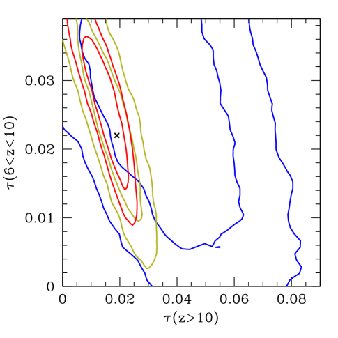

The key point illustrated in Figure 10 is that only CMBPol can strongly reject a significant high redshift contribution to the total optical depth. A strong limit on the high redshift contribution to the optical depth would rule out the presence of an early and efficient mode of star formation, and constrain the possible contribution of ionizing photons produced by annihilating or decaying dark matter. Alternatively, detecting a significant high redshift contribution would point to an exotic source of ionizing photons.
3.1.3 Constraints on the duration of reionization
Next we consider whether large scale polarization measurements can constrain the overall duration of the EoR, in addition to the redshift at which the IGM becomes half-neutral.
We use the simple two parameter model described in section 3.1.1. We explore two sets of parameters:
-
(i)
“Low model,” (,)=(10.5, 2.0), whose optical depth, , is close to the WMAP best-fitting value, [73],
-
(ii)
“High model,” (,)=(13.0, 3.5), whose optical depth, , is close to the upper 95% CL limit of the WMAP value.
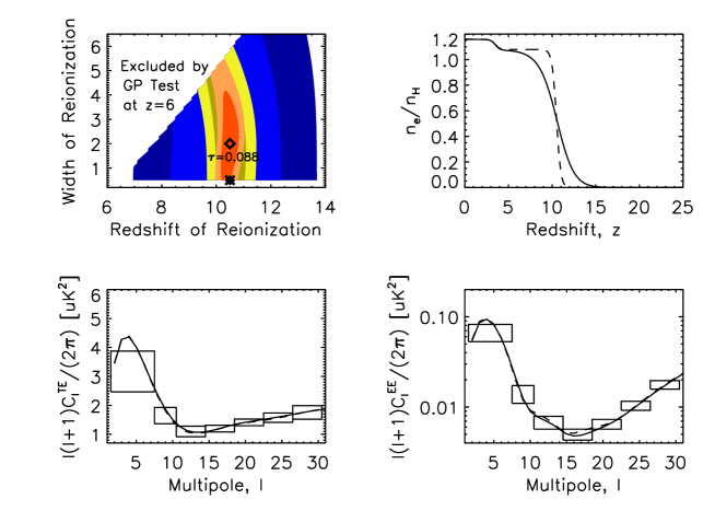
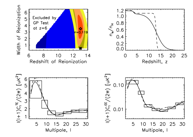
Figures 11 and 12 show the WMAP 5-year constraints (blue) and forecasts (yellow for Planck and orange for CMBPol) for the low and high optical depth scenarios. In the low model although Planck and CMBPol tightly constrains (as in §3.1.1), the duration of reionization, , is essentially unconstrained. Even the unphysical case of an instantaneous reionization model lies within the error contour. Models with large are either within the error contours, or are already excluded by quasar spectra (see §2.1). This is partly because the ionization history in this model is symmetric around . For instance, our current parametrization does not allow models where the ionization history rises abruptly for , but is more gradual above . In this case, one can constrain the high redshift contribution to the opacity, as we demonstrated in §3.1.2. In our high input model, one expects a weak constraint on the duration parameter, , from CMBPol. In this case, the instantaneous reionization and very rapid reionization models can be rejected at by CMBPol, although Planck can not distinguish such models. Unfortunately, it is hard to distinguish between more probable models with, e.g., and .
3.1.4 Constraints on a physical model
The ‘’ parametrization of the previous subsection is convenient, but somewhat arbitrary, and so we would like to explore an additional model to test whether this impacts our main conclusions. In this subsection we consider an alternate two parameter model for the reionization history. This model is also somewhat simplistic, but in combination with our previous model and the principle component analysis of §3.1.5, it should provide a good sense for CMBPol’s capabilities.
In the model of this section, the ionization fraction is directly related to the fraction of mass that is in dark matter halos above some minimum mass. This form is motivated by assuming that the star formation rate is proportional to the rate at which matter collapses into galactic host halos. See e.g. [80, 68] for a discussion of this model. More specifically, we assume that
| (3) |
Here the error function term, is the collapse fraction for halos with mass above according to Press-Schechter theory, is the linear theory overdensity for spherical top-hat collapse at redshift , extrapolated to today, is the linear growth factor, and is the variance of the linear density field extrapolated to today, and smoothed on a mass scale . We treat and as free parameters. The parameter is an efficiency parameter that depends physically on the number of ionizing photons produced per stellar baryon, the fraction of gas converted into stars, the fraction of ionizing photons that escape from host halos and make it into the IGM, as well as the average number of recombinations during reionization. This expression is similar to the form (with denoting the collapse fraction in halos above ) that is sometimes used, but our form goes smoothly to as becomes large. The parameter is the minimum mass for a halo to host an ionizing source. In reality and likely vary with redshift and environment, but we neglect this here in order to adopt a simple two parameter model.
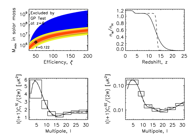
We computed a physical model which is tuned to have the same optical depth as the high model in the previous section; it turns out to have a roughly comparable spread in the reionization epoch as well. Fig. 13 shows that CMBPol can distinguish between the physical model and an instantaneous reionization model with the same at % CL. As in the parametrization, it is hard to distinguish models that have the same , yet different durations: only the instantaneous model can be rejected. This is seen in the contour plot as a degeneracy between very efficient yet rare source models (high , high ) where reionization occurs rapidly, and low efficiency abundant source models (low , low ) in which reionization is gradual. This supports the basic conclusion of the previous section: CMBPol can reject very rapid reionization models, but detailed constraints on the duration of reionization are impossible for smoothly varying reionization models.
3.1.5 Constraints on Principal components


The true reionization history may be more complex than the parametrized models of the previous two sub-sections. For example, feedback effects from the first generation of sources will likely impact the formation of subsequent galaxies and/or quasars, forcing the efficiency parameter and minimum host mass to vary with redshift and environment. If this is the case, one can hope to learn more about the reionization history than implied by the previous two sub-sections. In addition to the timing of reionization, and constraints on the high redshift contribution to the opacity, one may hope to learn further information regarding the duration of the reionization process. For instance, is the reionization process even monotonic?
As an example of a more general reionization history, we consider a double-peaked reionization history from Furlanetto & Loeb [81]. These authors investigate the conditions under which double-peaked reionization histories are physically plausible, and find that such histories require fine-tuning and are somewhat difficult to arrange, but not impossible. We hence adopt their model with a clumping factor of and a high virial temperature due to photoionization heating of K. The ionization history in this model, its -mode power spectrum with CMBPol error estimates, and the same for an instantaneous reionization model with the same () are shown in Figure 14. The instantaneous and double-peaked model can be distinguished at high significance (in excess of 3-). This illustrates that, if more freedom is allowed in the underlying reionization history than in the previous sub-sections, one can constrain more than just the total optical depth.
This motivates a more conservative approach that complements the constraints from the previous sub-sections. Here we allow to be a free function of redshift and see what constraints the data place on the form of this function with minimal theoretical assumptions. One simple implementation of this approach is to parametrize the ionization history using the values of in several wide redshift bins [82, 76]. An alternative parametrization that we employ here is principal components (PCs) of the ionization history, an orthogonal set of basis functions for ranked in order of how well they can be measured with large scale polarization data [83]. The interpretation of constraints on PCs is less intuitive than for the binned ionization fraction, but the advantages of PCs are that they are largely decorrelated from one another, there is less need for arbitrary redshift bin choices, and the impact of reionization on the CMB polarization is concentrated within a small number of the best measured components.
The principal components are defined as the eigenfunctions of the Fisher matrix that describes the information about reionization contained in the CMB polarization power spectrum on large scales [83],
where is large enough to include all effects of the mean ionization fraction, and the factor is included so that the eigenfunction shapes are independent of the initial redshift bin width as . The ordering of the PCs is based on their expected variances, given by the inverse eigenvalues of , , with the best constrained PCs having the lowest values of . For the set of PCs used here, we compute at a fiducial model of constant in redshift bins with spacing over a redshift range . The first five of these components are plotted on the left side of Fig. 15. The minimum redshift is motivated by observations of quasar absorption spectra. For details on how results depend on the chosen fiducial model and maximum redshift, , see Ref. [79]. The above equation assumes full sky coverage and sensitivity limited only by cosmic variance, but these choices have little effect on the PC shapes.

Any function of redshift between and can be expressed as a linear combination of PCs,
| (5) |
Only the lowest variance PCs affect the polarization power spectrum to a significant degree (i.e. larger than or comparable to cosmic variance) [83, 79]. One can therefore truncate the sum in Eq. (5) when estimating parameters from CMB data with while still retaining the full information about reionization present in the large scale polarization. For the results presented here and in § 3.1.2, we always use the five components plotted in Fig. 15 as parameters for MCMC analysis.
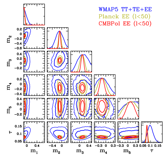
The right panel of Fig. 15 shows MCMC constraints on five PCs and the total optical depth from current and future CMB data. The largest set of contours are from five-year WMAP temperature and polarization power spectra, using MCMC estimates of the five reionization parameters in addition to the baryon density, CDM density, Hubble constant, and scalar amplitude and tilt [75]. Forecasted constraints on the five PCs from polarization at are plotted for Planck, assuming a sensitivity of K arcmin and beam size arcmin, and for a high resolution, cosmic variance limited experiment (“CMBPol”). The fraction of sky usable for cosmological constraints is assumed to be for both future experiments. We include the temperature data for WMAP since it provides some additional constraints to the current polarization data, but for Planck and CMBPol essentially all of the information about the mean ionization history can be obtained from the large scale polarization [79, 75]. To find the projected Planck and CMBPol parameter uncertainties we include polarization data up to since treating the ionization history as a free function up to high redshift allows for significant variation in at smaller scales than in typical parametrizations of reionization. For these forecasts, the amplitude of the temperature and polarization spectra at high is held fixed to the best fit to current data by keeping the value of fixed for each MCMC sample.
While the WMAP constraints in Fig. 15 come from real data and therefore reflect the true reionization history, we must choose the model for the simulated data used in the Planck and CMBPol forecasts. We take the fiducial ionization history to be the double-reionization model of Figure 14 and we compute MCMC likelihoods relative to the -mode polarization spectrum of this model. This fiducial model has a total optical depth of and a period of reionization extending from to . The estimates of and the principal component amplitudes recovered from the MCMC analysis agree well with the true parameter values of this input model.
The boundaries of plotted regions for the principal components on the right side of Fig. 15 are the edges of our priors on individual PCs. All potentially physical ionization histories (i.e. ) are included within these priors, including those that appear to violate the allowed range of when the sum of PCs is truncated [79]. However, this does not mean that every model inside these bounds is physically allowed or plausible. The PC priors are therefore in the spirit of the conservative approach to reionization constraints in which we allow for the largest conceivable variation in the ionization history.
If we allow the priors on PC amplitudes to define the range over which measurements enable interesting comparisons between models, then we find that current data places tight constraints on the first principal component, roughly corresponding to , and weakly limits the allowed range of the second component. Planck and CMBPol are expected to provide accurate estimates of several components: about for Planck and for cosmic variance limited CMBPol. Improvements in and the two lowest variance components between Planck and CMBPol are minimal, with most of the impact of having truly cosmic variance limited data appearing in the higher PCs.
It is important to note, however, that principal component parameters estimated at a significant level compared with the conservative priors do not necessarily lead to interesting constraints on physically motivated models. For many models of reionization that are currently thought to be realistic, the variation between models in higher variance PCs that undergo several oscillations in redshift is likely to be negligible. Therefore, the number of PCs that can be measured to an “interesting” level of precision depends on the range of possible variation in each of the components for the set of models being considered. Although a cosmic variance limited experiment is expected to measure components at a significant level compared with the full possible range when the ionization fraction is allowed to be a free function of redshift, under more restricted classes of models like those in § 3.1.4, it may be difficult to measure even two parameters at high significance.
Until observational limits on reionization and our theoretical understanding greatly improve our confidence in the specific behavior of the ionization fraction over time, it is worth keeping in mind that the true reionization scenario might be stranger than what we expect. Forecasts for models with a solid physical basis provide a realistic view of the advances we can expect from one experiment to the next, while the projected uncertainties on parameters like principal components that form a more model-independent description of the ionization history place an upper limit on the information about reionization that can be extracted from the CMB power spectra on large scales.
4 Impact of improved knowledge of reionization on other parameters
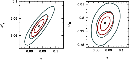
The determination for Planck will not be significantly degenerate with any other parameter apart from the amplitude of scalar perturbations and in some instances with the scalar–to–tensor ratio [76]. This is also true when a reconstruction of the reionization history from the data is attempted, however discrimination between specific reionization scenarios may be a challenge for Planck [84].
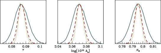
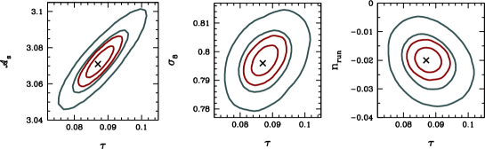
As for degeneracies, in such experiments would only be significantly degenerate with the amplitude of scalar perturbation and as a consequence with (see Fig.16). Even in non–minimal scenarios where an arbitrary scalar running spectral index and an free tensor spectral index are considered, does not show significant degeneracy with these parameters (Fig.17).
If CMBPol is able to measure the -mode polarization signature of gravitational waves from inflation, accurate estimates of reionization parameters will be necessary to avoid biasing constraints on inflationary parameters. Unless the amplitude of tensor perturbations is close to the current upper limit set by the CMB temperature data, the ability to probe inflation is likely to rely heavily on the reionization peak in the large scale -mode tensor spectrum since instrumental noise, angular resolution, and the conversion of -modes into -modes via lensing all present significant challenges for measuring on smaller scales. Without sufficient information about the reionization history from large scale -mode polarization, estimates of inflationary parameters such as the tensor-to-scalar ratio and tensor tilt that make use of the reionization peak in are strongly correlated with the total optical depth to reionization. Accurate constraints on and on the shape of the reionization history from cosmic variance limited measurements of would break this degeneracy, enabling the use of the large scale tensor contribution to for testing models of inflation [85].
5 Probing reionization with secondary anisotropies
5.1 Small angular scale measurements
On scales comparable to a tenth of a degree or smaller (), a second reionization observable comes into play, anisotropy created by the inhomogeneous distribution of ionized hydrogen (HII) surrounding the first sources. In this section we will discuss this probe and its potential to constrain not only the mean reionization redshift, but also its duration. Whether CMBPol or future ground based experiments will be the best platforms to do this measurement is currently unclear. A polarization mission which attempts to de-lens the polarization signal to reduce the lensing B-mode contamination requires high angular resolution and high sensitivity. Such a mission, if also sensitive to temperature anisotropies, would be ideal to study the secondary anisotropies generated during reionization.
There are two observables sourced by the inhomogeneous distribution of ionized hydrogen during the EoR. First note that anisotropies due to varying integrated optical depth lead to anisotropies in the observed power in different directions on the sky. Because in typical reionization models the sightline fluctuations are only of order , the contribution to the power spectrum is of order , which is below cosmic variance. 111111Even if one attempted to measure this contribution in one broad band power.
The dominant small scale CMB reionization observable comes instead from the fact that the extended ionized bubbles (which are about across at the intermediate EoR stages, leading to typical signatures of size on the sky) are embedded in large scale line-of-sight velocity flows. While the standard Ostriker-Vishniac/kinetic Sunyaev-Zel’dovich (SZ) effect [86, 87], owing to homogeneously ionized gas, is suppressed at these high redshifts, due to relatively low gas temperatures and small density contrasts, the inhomogeneity of ionized hydrogen adds a large contrast to the signal. The effect has been modeled in various ways [88, 89, 90, 91, 92]. In [91, 92] the signal was found to peak at , where it is still almost two orders of magnitude below the primary CMB signal. It is approximately one order of magnitude below the primary fluctuations at , and becomes the dominant contribution over the lensed primary CMB at , depending on the details of the reionization model and on how well the thermal Sunyaev-Zel’dovich effect [93] can be removed from the data (see Figure 18). The height of the “patchy reionization bump” (to be contrasted with the large scale bump in polarization discussed in the last section) depends on the total extent of the epoch, and its width depends on how much time the ionized fraction spends in various phases. If, for example, reionization stalls in its late stages, there will be relatively more large bubbles.

In [91] it was shown that already at Planck sensitivity patchy reionization can bias inferred cosmological parameter values if it is ignored, in particular if only temperature data are used. In polarization, secondary anisotropies are expected to be suppressed (see e.g. [94, 89]) by 4 orders of magnitude compared to the primary component. We make the approximation that the patchy reionization signal is unpolarized. The reason temperature data can be biased is that the broad bump seen in figure 18 enhances the power on small angular scales and, if not taken into account in the modeling, leads to (for example) an inferred primordial fluctuation spectrum that is bluer than it really is. The bias can be avoided either by only measuring temperature fluctuations out to , or by including an extra parameter for reionization to marginalize over, hoping that this parameter will not degrade the constraints on other parameters much. We go the second route here, and investigate parameter constraints possible with full CMBPol temperature and polarization information.
In this calculation we assume a raw detector noise level of K-arcmin and . We model reionization following the fast semi-analytic scheme of [66, 91]. Here we applied this model in a 1 comoving Gpc/h simulation volume with volume elements. We also go beyond previous work in that we vary the threshold for overdensities to be ionized throughout the box while translating between comoving position and redshift, thereby creating a model of “reionization on the light cone”. The redshift extent of the simulation box covers the entire reionization process. Modeling such a large volume in a full radiative transfer simulation would be prohibitive because of the requirement of a large dynamical range to model both the sources and large scales of reionization. However the size is particularly important for modeling the kinetic SZ effect because the velocity power spectrum peaks on scales of 250 Mpc/h. Our fiducial model, which will be used as template in the Fisher matrix analysis below, has a value for the ionization efficiency of 15, which leads in our concordance cosmology to an ionization fraction of 0.5 at z=11. To obtain a template for the patchy kSZ signal, we integrate the kinetic SZ signal
| (6) |
with
| (7) |
where the Thomson scattering optical depth is , is the optical depth from the observer to conformal time , and is the line of sight unit vector.
Assuming that the total duration of the EoR is long compared to the scale corresponding to the peak of the velocity power spectrum, we can make the approximation that if reionization takes e.g. twice as long to proceed, the r.m.s. of the induced anisotropy will be larger and the power spectrum amplitude doubled. Therefore to first order a 10% constraint on the amplitude of the patchy reionization admixture to the total CMB power spectrum can be translated into a 10% constraint on the duration of the process.
We assume here that the thermal SZ component, which is roughly comparable to the kinetic component on large scales (see Fig. 18), can be cleaned sufficiently. This can be justified by the fact that at , which is where the patchy reionization contribution peaks, most of the thermal SZ signal stems from massive and hot clusters of mass and larger at low redshift (see e.g. Figures 5 and 6 of [95]). These large bright objects can hopefully be excised using the multi-frequency information of the experiment 121212The brightness of polarized foregrounds will make observations in multiple frequency bands, roughly covering the range most interesting for the SZ, a necessity for a future CMB mission aiming to study the primordial E and B mode signals., as well as X-ray data from ROSAT or planned missions like the Constellation-X or X-ray Evolving Universe Spectroscopy (XEUS) missions 131313For details on planned X-ray observato- ries see http://constellation.gsfc.nasa.gov/ and http://www.rssd.esa.int/index.php?project=XEUS.. Furthermore, the thermal SZ vanishes at 220 GHz, leaving an unobstructed view on the patchy reionization contribution to an experiment observing in this frequency band.
Table 2 shows constraints that can be obtained on 8 cosmological parameters including a running of the spectral index and the patchy reionization amplitude. One can see that Planck will not be able to place interesting constraints on the reionization model. In [91] an extended reionization model (their model C) was investigated which was able to bias Planck constraints more strongly and might be borderline detectable.
In the case of CMBPol we find most parameter biases to be large (first column), since they are all much more tightly constrained. When the patchy reionization “nuisance parameter” is included in the analysis, we see that CMBPol should be able to place sub-percent constraints on this amplitude parameter, see table 2.
Here we have not discussed how well CMBPol might be able to discern reionization models with different source properties. For example feedback processes [96] or recombinations [97] could lead to relatively larger/smaller typical bubble sizes, imprinting the characteristic bump in Figure 18 on larger/smaller scales (and changing the slope at high , where the reionization signal comes to dominate over the primordial CMB). Furthermore, the width of the patchy reionization “bump” will depend on how much time is spent in each partial ionization stage.
A number of ground based observatories with high angular resolution, in particular the South Pole Telescope (SPT)141414The website for SPT is http://spt.uchicago.edu/ and the Atacama Cosmology Telescope (ACT)151515http://physics.princeton.edu/act are presently beginning observations. These experiments will primarily target the CMB anisotropies on the scale of a few arcminutes, to constrain the thermal SZ and the kinetic SZ effects from clusters and large scale structure at lower redshift as well as gravitational lensing. They also may be able to detect the patchy reionization admixture on these scales.
| [fid. value] | , RefExp (Planck) | RefExp, | RefExp, |
|---|---|---|---|
| 2.70 (6.97) | 2.73 | 2.78 | |
| 0.30 (0.89) | 0.31 | 0.41 | |
| 0.41 (1.15) | 0.44 | 0. 56 | |
| 0.11 (0.68) | 0.12 | 0.23 | |
| [0.963] | 0.17 (0.47) | 0.18 | 0.21 |
| [] | 0.38 (1.22) | 0.48 | 0.52 |
| 0.20 (0.60) | 0.23 | 0.33 | |
| 0.42 (119.0) | 3.22 | 33.5 |
5.2 The effect of metals
As the first sources turn on an ionize the universe metals are also produced for the first time. These metals eventually enrich the inter-galactic medium (e.g. [98]). Here we concentrate on the resonant scattering signature of metal enrichment of the inter-galactic medium by the first stars on the CMB. CMB photons interacting with a species at redshift via a resonant transition of resonant frequency , show the effect of the interaction if [99]. The resonant scattering of this species generates an optical depth to CMB photons [100]: where is the number density of the species and is the absorption oscillator strength. modifies temperature anisotropies: In the limit of low metal abundance , we can retain only linear terms in . Thus as described in [99], the change in the anisotropies () reduces to a blurring factor () plus a new term which is important only in the large scales. The large scale signal is less clean to interpret than the high signal because at low multipoles generation and suppression terms tend to cancel out. The high signal in multipole space is [99]: , i.e. it is proportional to the primary anisotropies, with a well defined frequency dependence: in the presence of only one resonant species at the effect will be non-zero only at frequency . Thus the metals contribution to the power spectrum is proportional to the primordial CMB power spectrum with constant of proportionality given by .
In a given experiment, the lowest frequency channel corresponds to the highest redshift where the metal abundance is the lowest. Increments of metal abundances can be measured by studying the difference map and the difference power spectra between channels. Signal-to-noise considerations [101] show that the main limiting factor is the accuracy of the cross-channel calibration.
A purpose-built experiment with the properties of the EPIC 2m set up, with accurate control of systematics and cross-channel calibration might be sensitive to changes in 3-12% (2-) of the Solar fraction of Oxygen abundance at for reionizaton redshift (OIII m transition) and to changes in N abundance of 60% its solar value for (2-)(NII 205 m transition).
Appendix: Likelihood Function
For computing the constraints from the WMAP 5-year data, we shall evaluate the likelihood function directly in pixel space, following Appendix D of Page et al. (2007).
For forecasting parameter constraints from Planck and CMBPol, we shall evaluate the likelihood functions in harmonic space. The form of the likelihood function for a theoretical model, , given the data, , is
| (8) | |||||
where are the noisebias (which is assumed to be constant over multipoles) given by
| (9) | |||||
| (10) |
Here, and are the temperature and polarization sensitivities, respectively, which are related to “ per pixel” in Table 1.1 on pp.4 of the Planck Blue Book via
| (11) | |||||
| (12) | |||||
Note that we have ignored the effect of beam smearing, as we focus only on low multipoles where the beam effect may be ignored safely.
In our calculation we integrate the likelihood function up to , beyond which little information is available for reionization. When we compute the likelihood function for CMBPol, we shall assume that CMBPol is limited only by the cosmic variance up to , i.e., up to . On the other hand when we compute the likelihood function for Planck, we shall combine the sensitivities in 70 GHz (LFI), 100 GHz (HFI), and 143 GHz (HFI), such that
| (13) | |||||
| (14) |
From the Planck Blue Book we find , and . Therefore, the combined sensitivities for Planck are given by
| (15) | |||||
| (16) |
and thus we find
| (17) | |||||
| (18) |
References
- [1] E. Komatsu et al. [WMAP Collaboration], arXiv:0803.0547 [astro-ph].
- [2] Wyithe, J. S. B., & Loeb, A. 2003, ApJ Lett., 588, L69
- [3] Cen, R. 2003, ApJ Lett., 591, L5
- [4] Haiman, Z., & Holder, G. P. 2003, ApJ, 595, 1
- [5] Mackey, J., Bromm, V., & Hernquist, L. 2003, ApJ, 586, 1
- [6] Yoshida, N., Abel, T., Hernquist, L., & Sugiyama, N. 2003, ApJ, 592, 645
- [7] Yoshida, N., Bromm, V., & Hernquist, L. 2004, ApJ, 605, 579
- [8] Sokasian, A., Abel, T., Hernquist, L. & Springel, V. 2003, MNRAS, 344, 607
- [9] Sokasian, A., Yoshida, N., Abel, T., Hernquist, L. & Springel, V. 2004, MNRAS, 350, 47
- [10] Yoshida, N., Omukai, K., Hernquist, L. & Abel, T. 2006, ApJ, 652, 6
- [11] Zaldarriaga, M. 1997, Phys. Rev. D, 55, 1822
- [12] Kaplinghat, M., Chu, M., Haiman, Z., Holder, G. P., Knox, L., & Skordis, C. 2003, ApJ, 583, 24
- [13] Hu, W., & Holder, G. P. 2003, Phys. Rev. D, 68, 23001
- [14] M. McQuinn, A. Lidz, O. Zahn, S. Dutta, L. Hernquist & M. Zaldarriaga Mon. Not. Roy. Astron. Soc. 377, 1043 (2007) [arXiv:astro-ph/0610094].
- [15] O. Zahn, A. Lidz, M. McQuinn, S. Dutta, L. Hernquist, M. Zaldarriaga & S. R. Furlanetto, Astrophys. J. 654, 12 (2006) [arXiv:astro-ph/0604177].
- [16] Becker, R. H., et al. 2001, AJ, 122, 2850
- [17] X. H. Fan et al., Astron. J. 132, 117 (2006) [arXiv:astro-ph/0512082].
- [18] Songaila, A. 2004, AJ, 127, 2598
- [19] Becker, G. D., Rauch, M., & Sargent, W. L. W. 2006, astro-ph/06070633
- [20] Miralda-Escudé, J., Haehnelt, M., & Rees, M. J. 2000, ApJ, 530, 1
- [21] Oh, S. P., & Furlanetto, S. R., 2005, ApJL, 620, 9
- [22] Lidz, A., Oh, S. P., & Furlanetto, S. R. 2006, ApJL, 639, 47
- [23] Wyithe, J. S. B., & Loeb, A. 2006, ApJ, 646, 696
- [24] Liu, J., Bi, H., Feng, L. L., & Fang, L. Z., 2006, ApJL, 645, 1
- [25] J. S. B. Wyithe & A. Loeb 2004, arXiv:astro-ph/0401188.
- [26] J. S. B. Wyithe, A. Loeb & C. Carilli, Astrophys. J. 628, 575 (2005) [arXiv:astro-ph/0411625].
- [27] A. Mesinger & Z. Haiman, arXiv:astro-ph/0610258.
- [28] J. S. Bolton & M. G. Haehnelt, Mon. Not. Roy. Astron. Soc. 374, 493 (2007) [arXiv:astro-ph/0607331].
- [29] A. Lidz, M. McQuinn & M. Zaldarriaga Astrophys. J. 670, 39 (2007) [arXiv:astro-ph/0703667].
- [30] Ryan-Webber, E. V., Pettini, M., & Madau, P., 2006, MNRAS, 371L, 78
- [31] Simcoe, R. A., 2006, ApJ, 653, 977
- [32] Oh, S. P. 2002, MNRAS, 336, 1021
- [33] Becker, G. D., Sargent, W. L. W., Rauch, M., & Simcoe, R. A. 2006, ApJ, 640, 69
- [34] Theuns, T., et al. 2002, ApJ Lett., 567, L103
- [35] Hui, L., & Haiman, Z. 2003, ApJ, 596, 9
- [36] Sokasian, A., Abel, T., & Hernquist, L. 2002, MNRAS, 332, 601
- [37] McQuinn, M., Lidz, A., Zaldarriaga, M., Hernquist, L., Hopkins, P. F., Dutta, S., & Faucher-Giguere, C. A., 2008, arXiv:0807.2799
- [38] Kohler, K., Gnedin, N. Y., & Hamilton, A. J. S., 2007, ApJ, 657, 15
- [39] Trac, H., Cen, R., & Loeb, A. 2008, ApJL submitted, arXiv:0807.4530
- [40] Partridge, R. B., & Peebles, P. J. E. 1967, ApJ, 147, 868
- [41] Hu, E. M., et al. 2002, ApJ Lett., 568, L75
- [42] Kodaira, K., et al. 2003, Pub. Astron. Soc. Japan, 55, 232
- [43] Rhoads, J. E., et al. 2004, ApJ, in press (astro-ph/0403161)
- [44] Stanway, E. R., et al. 2004, ApJ Lett., 604, L13
- [45] Santos, M. R., et al. 2004, ApJ, 606, 683
- [46] Kashikawa N., et al., 2006, ApJ, 648, 7
- [47] Cuby J.-G., Hibon P., Lidman C., Le Fèvre O., Gilmozzi R., Moorwood A., van der Werf P., 2007, A& A, 461, 911
- [48] Willis J. P., Courbin F., 2005, MNRAS, 357, 1348
- [49] D. P. Stark, R. S. Ellis, J. Richard, J. P. Kneib, G. P. Smith & M. R. Santos, arXiv:astro-ph/0701279.
- [50] Casali M., et al., 2006, in Ground-based and Airborne Instrumentation for Astronomy. Edited by McLean, Ian S.; Iye, Masanori. Proceedings of the SPIE, Volume 6269, pp. (2006). HAWK-I: the new wide-field IR imager for the VLT
- [51] McPherson A. M., et al., 2006, in Ground-based and Airborne Telescopes. Edited by Stepp, Larry M.. Proceedings of the SPIE, Volume 6267, pp. (2006). VISTA: project status
- [52] Horton A., Parry I., Bland-Hawthorn J., Cianci S., King D., McMahon R., Medlen S., 2004, PROC.SPIE INT.SOC.OPT.ENG., 5492, 1022
- [53] McQuinn, M., Hernquist, L., Zaldarriaga, M., & Dutta, S. 2007, MNRAS, 381, 75
- [54] Miralda-Escudé, J. 1998, ApJ, 501, 15
- [55] Furlanetto, S. R., Zaldarriaga, M., & Hernquist, L. 2006, MNRAS, 365, 1012
- [56] Mesinger, A., & Furlanetto, S. R., 2007, MNRAS in press, arXiv:0708.0006
- [57] Malhotra, S. & Rhoads, J. E., 2006, ApJL, 647, 95
- [58] Dijkstra, M., Wyithe, J. S. B., & Haiman, Z., 2007, MNRAS, 379, 253
- [59] Fernandez, E. R., & Komatsu, E., 2008, MNRAS, 384, 1363
- [60] Barkana, R., & Loeb, A., 2004, ApJ, 601, 64
- [61] Totani, T., Kawai, N., Kosugi, G., Aoki, K., Yamada, T., Iye, M., Ohta, K., & Hattori, T., 2006, PASJ, 58, 485
- [62] M. McQuinn, A. Lidz, M. Zaldarriaga, L. Hernquist & S. Dutta, arXiv:0710.1018 [astro-ph].
- [63] Chen, H. -W., Prochaska, J. X., & Gnedin, N. Y. 2007, ApJL, 667, 125
- [64] X. L. Chen & J. Miralda-Escudé 2004, Astrophys. J. 602, 1
- [65] Ciardi, B., & Madau, P., 2003, ApJ, 596, 1
- [66] S. Furlanetto, M. Zaldarriaga & L. Hernquist, Astrophys. J. 613, 1 (2004) [arXiv:astro-ph/0403697].
- [67] Iliev, I. T., Mellema, G., Pen, U. L., Bond, J. R., & Shapiro, P. R. 2008, MNRAS, 384, 863
- [68] Furlanetto, S. R., Oh, S. P., & Briggs, F. 2006, Phys. Reports, 433, 181
- [69] M. McQuinn, O. Zahn, M. Zaldarriaga, L. Hernquist & S. R. Furlanetto, Astrophys. J. 653, 815 (2006) [arXiv:astro-ph/0512263].
- [70] A. Lidz, O. Zahn, M. McQuinn, M. Zaldarriaga & L. Hernquist, arXiv:0711.4373 [astro-ph].
- [71] Pritchard, J. R., & Furlanetto, S. R. 2007, MNRAS, 376, 1680
- [72] M. Zaldarriaga, S. R. Furlanetto & L. Hernquist 2004, ApJ, 608, 622
- [73] J. Dunkley et al. [WMAP Collaboration], arXiv:0803.0586 [astro-ph].
- [74] L. P. L. Colombo e; al. In preparation.
- [75] M. J. Mortonson & W. Hu, ApJ Lett., 686, L53 (2008) [arXiv:0804.2631].
- [76] L. P. L. Colombo & E. Pierpaoli, arXiv:0804.0278 [astro-ph].
- [77] B. P. Crill et al., arXiv:0807.1548 [astro-ph].
- [78] J. Bock et al., arXiv:0805.4207 [astro-ph].
- [79] M. J. Mortonson & W. Hu, Astrophys. J. 672, 737 (2008) [arXiv:0705.1132 [astro-ph]].
- [80] Alvarez, M. A., Komatsu, E., Doré, O., & Shapiro, P. R. 2006, ApJ, 647, 840
- [81] S. Furlanetto & A. Loeb, Astrophys. J. 634, 1 (2005) [arXiv:astro-ph/0409656].
- [82] A. Lewis, J. Weller & R. Battye, Mon. Not. Roy. Astron. Soc. 373, 561 (2006) [arXiv:astro-ph/0606552].
- [83] Hu, W., & Holder, G. P. 2003, Phys. Rev. D, 68, 23001
- [84] P. Mukherjee & A. R. Liddle, arXiv:0803.1738 [astro-ph].
- [85] M. J. Mortonson & W. Hu, Phys. Rev. D 77, 043506 (2008) [arXiv:0710.4162 [astro-ph]].
- Ostriker & Vishniac [1986] Ostriker, J. & Vishniac, E. 1986, ApJ, 306, 51
- Sunyaev & Zel’dovich [1980] Sunyaev, R. A. & Zel’dovich, Y. B. 1980, MNRAS, 190, 413
- Knox et al. [1998] Knox, L., Scoccimarro, R., & Dodelson, S. 1998, Phys. Rev. Lett., 81, 2004
- [89] W. Hu, Astrophys. J. 529, 12 (2000) [arXiv:astro-ph/9907103].
- Santos et al. [2003] Santos, M. G., Cooray, A., Haiman, Z., Knox, L., & Ma, C.-P. 2003, ApJ, 598, 756
- Zahn et al. [2005] Zahn, O., Zaldarriaga, M., Hernquist, L., & McQuinn, M. 2005, ApJ, 630, 657, astro-ph/0503166
- McQuinn et al. [2005] McQuinn, M., Furlanetto, S. R., Hernquist, L., Zahn, O., & Zaldarriaga, M. 2005, ApJ, 630, 643, astro-ph/0504189
- Zel’dovich & Sunyaev [1969] Zel’dovich, Y. B. & Sunyaev, R. A. 1969, Astrophys. Space Sci., 4, 301
- [94] S. Y. Sazonov & R. A. Sunyaev, Mon. Not. Roy. Astron. Soc. 310, 765 (1999) [arXiv:astro-ph/9903287].
- [95] E. Komatsu & U. Seljak, Mon. Not. Roy. Astron. Soc. 336, 1256 (2002) [arXiv:astro-ph/0205468].
- Furlanetto et al. [2006a] Furlanetto, S. R., McQuinn, M., & Hernquist, L. 2006a, MNRAS, 365, 115, astro-ph/0507524
- Furlanetto & Oh [2005] Furlanetto, S. R., & Oh, S. P. 2005, MNRAS, 363, 103, astro-ph/0505065
- [98] Barkana R., Loeb A., 2001, PhR, 349, 125
- [99] Basu, K., Hernández-Monteagudo, C., & Sunyaev, R. A. 2004, A& A, 416, 447
- [100] Sobolev, V.V. 1946, Moving Atmospheres of Stars (Lenningrad: Leningrad State Univ.; English transl.1960, Cambridge:Harvard Univ. Press)
- [101] Hernández-Monteagudo, C., Verde, L., Jimenez, R. 2006, ApJ, 653, 10.