Lie-Semigroup Structures for Reachability and Control of Open Quantum Systems:
Kossakowski-Lindblad Generators Form Lie Wedge to Markovian Channels

Zusammenfassung

In view of controlling finite dimensional open quantum systems, we provide a unified Lie-semigroup framework describing the structure of completely positive trace-preserving maps. It allows (i) to identify the Kossakowski-Lindblad generators as the Lie wedge of a subsemigroup, (ii) to link properties of Lie semigroups such as divisibility with Markov properties of quantum channels, and (iii) to characterise reachable sets and controllability in open systems. We elucidate when time-optimal controls derived for the analogous closed system already give good fidelities in open systems and when a more detailed knowledge of the open system (e.g., in terms of the parameters of its Kossakowski-Lindblad master equation) is actually required for state-of-the-art optimal-control algorithms. As an outlook, we sketch the structure of a new, potentially more efficient numerical approach explicitly making use of the corresponding Lie wedge.

Key-Words: completely positive quantum maps, Markovian quantum channels, divisibility in semigroups, Kossakowski-Lindblad generators, invariant cones; optimal control, gradient flows.

PACS Numbers: 02.30.Yy, 02.40.Ky, 02.40.Vh, 02.60.Pn; 03.65.Yz, 03.67.-a, 03.67.Lx, 03.65.Yz, 03.67.Pp; 42.50.Dv; 76.60.-k, 82.56.-b

I Introduction

Understanding and manipulating open quantum systems and quantum channels is an important challenge for exploiting quantum effects in future technology Dowling and Milburn (2003).

Protecting quantum systems against relaxation is therefore tantamount to using coherent superpositions as a resource. To this end, decoherence-free subspaces have been applied Zanardi and Rasetti (1998), bang-bang controls Viola et al. (2000) have been used for decoupling the system from dissipative interaction with the environment, while a quantum Zeno approach Misra and Sudarshan (1977) may be taken to projectively keep the system within the desired subspace Facchi and Pascazio (2001). Very recently, the opposite approach has been taken by solely expoiting relaxative processes for state preparation Verstraete et al. (2008); Büchler et al. (2008). It is an extreme case of engineering quantum dynamics in open systems Viola and Lloyd (2001), where targeting fix points has lately become of interest Bertlman et al. (2008).

In either case, for exploiting the power of system and control theory, first the quantum systems has to be characterised, e.g., by input-output relations in the sense of quantum process tomography. Deciding whether the dynamics of the quantum system thus specified allows for a Markovian description to good approximation (maybe up to a certain level of noise) has recently been addressed Wolf and Cirac (2008); Wolf et al. (2008); Wolf (2008). This is of crucial interest, since a Markovian equation of motion paves the way to applying the power Lie-theoretic methods Jurdjevic and Sussmann (1972); Jurdjevic (1997) from geometric and bilinear control theory. Moreover, it comes with the well-established frameworks of completely positive semigroups and Kraus representations Kraus (1971); Kossakowski (1972a, b); Choi (1975); Gorini et al. (1976); Lindblad (1976); Kraus (1983); Wu et al. (2007).

On the other hand, the specific Lie-semigroup aspects of open quantum systems clearly have not been elaborated on in the pioneering period 1971–76 of completely positive semigroups Kossakowski (1972a, b); Gorini et al. (1976); Lindblad (1976); Davies (1976), mainly since major progress in the understanding of Lie semigroups was made in the decade 1989–99 Hilgert et al. (1989); Eggert (1991a); Neeb (1992); Hilgert and Neeb (1993); Hofmann et al. (1995); Hofmann and Ruppert (1997). While relations of Lie semigroups and classical control theory were soon established, e.g., in Jurdjevic and Kupka (1981a, b); Hofmann and Ruppert (1983); Hofmann and Ruppert (1991a); Mittenhuber (1994); Hofmann et al. (1995); Mittenhuber (1995); Lawson (1999), only recently the use of Lie-semigroup terms in the control of open quantum systems was initiated Altafini (2003); Dirr and Helmke (2008), where in Altafini (2003) the elaborations were confined to single two-level systems. However, we see a great potential in exploiting the algebraic structure of Lie-semigroup theory for practical problems of reachability and control of open quantum systems.

Its importance becomes evident, because among the generic tools needed for the current advances in quantum technology (for a survey see, e.g., Dowling and Milburn (2003)), quantum control plays a major role. From formal description of quantum optimal control Butkovskiy and Samoilenko (1990) the theoretical aspects of existence of optima soon matured into numerical algorithms solving practical problems of steering quantum dynamics Peirce et al. (1987); Dahleh et al. (1990); Krotov (1996); Khaneja et al. (2005). Their key concern is to find optima of some quality function like the quantum gate fidelity under realistic conditions and, moreover, constructive ways of achieving those optima given the constraints of an accessible experimental setting. For a recent introduction, see D’Alessandro (2008). However, realistic implementations in open quantum systems are mostly beyond analytical tractability. Hence numerical methods are often indispensible, where gradient-like algorithms are the most basic, but robust tools. Thus they proved applicable to a broad array of problems including optimal control of closed quantum systems Khaneja et al. (2005); Dirr et al. (2006a) and computing entanglement measures Schulte-Herbrüggen et al. (2008a); Dirr et al. (2006b); Curtef et al. (2008). For mathematical details on gradient systems as numerical tools for constrained optimisation, we refer to Brockett (1988); Bloch (1994); Helmke and Moore (1994).

Generalising these well-established gradient techniques, in our previous work Schulte-Herbrüggen et al. (2008a), we have exploited the geometry of Riemannian manifolds related to Lie groups, their subgroups, and homogeneous spaces in a common framework for setting up gradient flows in closed quantum systems. There we addressed (a) abstract optimisation tasks on smooth state-space manifolds and (b) dynamic optimal control tasks in the specific time scales of an experimental setting. Here, we will see that the corresponding abstract optimisation tasks for open quantum systems are much more involved, while the dynamic optimal control tasks remain in principle the same. From a mathematical point of view, this difficulty results from the fact that the evolution of a controlled open quantum system is no longer described by a semigroup of unitary propagators, i.e. by a semigroup contained in a compact Lie group.

Thus, we extend the Lie-theoretic approach in Schulte-Herbrüggen et al. (2008a) to finite dimensional open quantum systems and discuss their dynamics in terms of Lie semigroups. In particular, we characterise the Lie properties (the Lie wedge) of Markovian quantum channels from the viewpoint of divisibility and local divisibility in semigroups. — On a general scale and with regard to practical applications of quantum control, knowing about the Lie-semigroup structure of the dynamic system is shown to be highly advantageous: analysing its tangent cones (Lie wedges) allows for addressing problems of reachability, accessibility, controllability and actual control in a unified frame providing powerful Lie algebraic terms.

Starting Point

To begin with, we briefly indicate how the theory elucidated in previous work Schulte-Herbrüggen et al. (2008a) can be extended to reachable sets of non necessarily controllable systems. In particular, we concentrate on the structure of reachable sets and obstacles arising from it. Moreover, pertinent applications to open relaxative quantum dynamical systems are elaborated—proving the relevance of the semigroup setting in physics.

The starting point in Schulte-Herbrüggen et al. (2008a) was a smooth state-space manifold $M$ or a controllable dynamical system on $M$, i.e. a control system whose reachable sets $\operatorname{Reach}(X_{0})$ satisfy $\operatorname{Reach}(X_{0})=M$ for all $X_{0}\in M$. For a right invariant system (4) the state space of which is given by a connected Lie group $\mathbf{G}$, controllability is equivalent to the fact that the entire group $\mathbf{G}$ can be reached from the unity ${\rm 1\negthickspace l}{}$, i.e.

$$\mathbf{G}=\operatorname{Reach}({\rm 1\negthickspace l}{}):=\bigcup_{T\geq 0}\operatorname{Reach}({\rm 1\negthickspace l}{},T),$$ (1)

where $\operatorname{Reach}({\rm 1\negthickspace l}{},T)$ denotes the reachability set in time $T\geq 0$, i.e. the set of all states to where the systems can be steered from ${\rm 1\negthickspace l}{}\in\mathbf{G}$ in time $T$, cf. Eqn.(5). In general, however, we cannot expect Eqn.(1) to hold. Nevertheless, the reachability sets $\operatorname{Reach}({\rm 1\negthickspace l}{},T_{1})$ and $\operatorname{Reach}({\rm 1\negthickspace l}{},T_{2})$ of right invariant systems obey the following multiplicative structure

$$\operatorname{Reach}({\rm 1\negthickspace l}{},T_{1})\cdot\operatorname{Reach}({\rm 1\negthickspace l}{},T_{2})=\operatorname{Reach}({\rm 1\negthickspace l}{},T_{1}+T_{2}).$$

Thus $\operatorname{Reach}({\rm 1\negthickspace l}{})$ is a subsemigroup of $\mathbf{G}$, see Sec.II.4. — Now, we will give a basic survey on subsemigroups and some of their applications in quantum control.

II Fundamentals of Lie Subsemigroups and Reachable Sets

II.1 Lie Subsemigroups

For the following basic definitions and results on Lie subsemigroups we refer to Hilgert and Neeb (1993); Hilgert et al. (1989); Hofmann (1991); Eggert (1991b); Neeb (1991). However, the reader should be aware of the fact that the terminology in this area is sometimes inconsistent. Here, we primarily adopt the notions used in Hilgert and Neeb (1993). For further reading we also recommend Lawson (1999).

A subsemigroup of a (matrix) Lie group $\mathbf{G}$ with Lie algebra $\mathfrak{g}$ is a subset $\mathbf{S}\subset\mathbf{G}$ which contains the unity ${\rm 1\negthickspace l}{}$ and is closed under multiplication, i.e. $\mathbf{S}\cdot\mathbf{S}\subseteq\mathbf{S}$. The largest subgroup contained in $\mathbf{S}$ is denoted by ${\rm E}(\mathbf{S}):=\mathbf{S}\cap\mathbf{S}^{-1}$. The tangent cone of $\mathbf{S}$ is defined as

$${\rm L}(\mathbf{S}):=\{\dot{\gamma}(0)\;|\;\mbox{$\gamma(0)={\rm 1\negthickspace l}{}$, $\gamma(t)\in\mathbf{S}$, $t\geq 0$}\}\subset\mathfrak{g},$$

where $\gamma:[0,\infty)\to\mathbf{G}$ denotes any smooth curve contained in $\mathbf{S}$. In order to relate subsemigroups to their tangent cones, we need some further terminology from convex analysis. A closed convex cone $\mathfrak{w}$ of a finite dimensional real vector space is called a wedge.

Moreover, a wedge $\mathfrak{w}$ in a Lie algebra $\mathfrak{g}$ is termed a Lie semialgebra if the wedge $\mathfrak{w}$ is locally compatible with the Baker-Campbell-Hausdorff (bch) multiplication $X*Y:=X+Y+\tfrac{1}{2}[X,Y]+\dots$, defined via the bch series. More precisely, there has to be an open bch neighbourhood $B\subset\mathfrak{g}$ of $0$ such that $\mathfrak{w}$ is locally invariant under $*$, i.e.

$$(\mathfrak{w}\cap B)*(\mathfrak{w}\cap B)\subseteq\mathfrak{w}.$$ (2)

For a thorough treatment of the bch multiplication and Lie semialgebras see Hilgert et al. (1989); Eggert (1991a).

The edge of $\mathfrak{w}$ denoted by ${\rm E}(\mathfrak{w})$ is the largest subspace contained in $\mathfrak{w}$, i.e. one has ${\rm E}(\mathfrak{w}):=\mathfrak{w}\cap(-\mathfrak{w})$. Finally, a wedge $\mathfrak{w}$ of a finite dimensional real (matrix) Lie algebra $\mathfrak{g}$ is called a Lie wedge if it is invariant under the group of inner automorphisms $\mathbf{Inn(\mathfrak{w})}:=\langle\exp(\operatorname{ad}_{{\rm E}(\mathfrak{w})})\rangle$. More precisely,

$${\rm e}^{\operatorname{ad}_{g}}(\mathfrak{w}):={\rm e}^{g}\,\mathfrak{w}\,{\rm e}^{-g}=\mathfrak{w}$$

for all $g\in{\rm E}(\mathfrak{w})$. Here and in the sequel, we denote by $\langle M\rangle$ and $\langle M\rangle_{S}$ the group and, respectively, semigroup generated by the subset $M\subset\mathbf{G}$.

Remark II.1.

While every Lie semialgebra is also a Lie wedge, the converse does in general not hold, as will be of importance in the paragraph on divisibility in Sec. II.3.

Now, the fundamental properties of the tangent cone ${\rm L}(\mathbf{S})$ can be summarised as follows.

Lemma II.1.

Let $\mathbf{S}$ be a closed subsemigroup of a Lie group $\mathbf{G}$ with Lie algebra $\mathfrak{g}$ and let $\mathfrak{w}\subset\mathfrak{g}$ be any Lie wedge. Then the following statements are satisfied.

1. The edge of $\mathfrak{w}$, ${\rm E}(\mathfrak{w})$, carries the structure of a Lie subalgebra of $\mathfrak{g}$.

2. The tangent cone ${\rm L}(\mathbf{S})$ coincides with

   $${\rm L}(\mathbf{S})=\{g\in{\mathfrak{g}}\,|\,\mbox{$\exp(tg)\in\mathbf{S}$ for all $t\geq 0$}\}.$$ (3)

   In particular, ${\rm L}(\mathbf{S})$ is a Lie wedge of $\mathfrak{g}$ which is $\mathrm{Ad}_{{\rm E}(\mathbf{S})}$-invariant, i.e. $G\mathfrak{w}G^{-1}=\mathfrak{w}$ for all $G\in{\rm E}(\mathbf{S})$.

3. The edge of ${\rm L}(\mathbf{S})$ fulfills the equality ${\rm E}({\rm L}(\mathbf{S}))={\rm L}({\rm E}(\mathbf{S}))$.

Proof.

1. Note that ${\rm e}^{t\operatorname{ad}_{g}}(h)\in{\rm E}(\mathfrak{w})$ for all $t\in\mathbb{R}$ and $g,h\in{\rm E}(\mathfrak{w})$. Hence

   $$\frac{\rm d}{{\rm d}t}{\rm e}^{t\operatorname{ad}_{g}}(h)\big{|}_{t=0}=\operatorname{ad}_{g}h\in{\rm E}(\mathfrak{w})$$

   for all $g,h\in{\rm E}(\mathfrak{w})$, thus ${\rm E}(\mathfrak{w})$ is a Lie subalgebra.

2. The proof of Eqn. (3) is rather technical and therefore we refer to Hilgert et al. (1989), Proposition IV.1.21. Once Eqn. (3) is established, one has

   $${\rm L}(\mathbf{S})=\bigcap_{t>0}t^{-1}\exp^{-1}(\mathbf{S})$$

   and thus the continuity of the exponential map implies that ${\rm L}(\mathbf{S})$ is closed. To see that ${\rm L}(\mathbf{S})$ is a wedge we have to show: (i) $\mu{\rm L}(\mathbf{S})={\rm L}(\mathbf{S})$ for all $\mu\in\mathbb{R}^{+}$ and (ii) ${\rm L}(\mathbf{S})+{\rm L}(\mathbf{S})\subset{\rm L}(\mathbf{S})$. Property (i) is obvious; property (ii) follows by the Trotter product formula

   $${\rm e}^{t(g+h)}=\lim_{n\to\infty}\big{(}{\rm e}^{tg/n}{\rm e}^{th/n}\big{)}^{n}.$$

   Finally, let $g\in{\rm E}({\rm L}(\mathbf{S}))$ and $h\in{\rm L}(\mathbf{S})$, then

   $${\rm e}^{g}e^{th}{\rm e}^{-g}=\exp\big{(}t\,{\rm e}^{g}\,h\,{\rm e}^{-g}\big{)}\in\mathbf{S}$$

   for all $t\geq 0$. Thus ${\rm e}^{g}h{\rm e}^{-g}={\rm e}^{\operatorname{ad}_{g}}(h)\in{\rm L}(\mathbf{S})$. The same argument applies to $G\in{\rm E}(\mathbf{S})$.

3. Let $g\in{\rm E}({\rm L}(\mathbf{S}))$. Then ${\rm e}^{tg}\in\mathbf{S}$ for all $t\in\mathbb{R}$. Thus ${\rm e}^{tg}\in{\rm E}(\mathbf{S})$ and hence $g\in{\rm L}({\rm E}(\mathbf{S}))$. Therefore, we have shown ${\rm E}({\rm L}(\mathbf{S}))\subset{\rm L}({\rm E}(\mathbf{S}))$. The converse, ${\rm L}({\rm E}(\mathbf{S}))\subset{\rm E}({\rm L}(\mathbf{S}))$, holds by definition.

   For more details, see Proposition 1.14 in Hilgert and Neeb (1993). $\blacksquare$

For closed subsemigroups, Lemma II.1 provides the justification to call the tangent cone ${\rm L}(\mathbf{S})$ Lie- or Lie-Loewner wedge of $\mathbf{S}$.

Unfortunately, the ‘local-global-correspondence’ between Lie wedges and (closed) connected subsemigroups is not as simple as the correspondence between Lie subalgebras and Lie subgroups. On the one hand, there are Lie wedges $\mathfrak{w}$ such that ‘the’ corresponding subsemigroup $\mathbf{S}$ is not unique, i.e. the equality $\mathfrak{w}={\rm L}(\mathbf{S})$ holds for more than one subsemigroup $\mathbf{S}$. On the other hand, there are Lie wedges $\mathfrak{w}$ which do not act as Lie wedge of any subsemigroup, i.e. $\mathfrak{w}={\rm L}(\mathbf{S})$ fails for each subsemigroup $\mathbf{S}$, cf. Hilgert and Neeb (1993).

Another subtlety in the theory of semigroups arises from the fact that there may exist elements in $\mathbf{S}$ that are arbitrarily close to the unity but do not belong to any one-parameter semigroup completely contained in $\mathbf{S}$ (a standard example being a certain subsemigroup of the Heisenberg group Hilgert et al. (1989); Hofmann and Ruppert (1997)). This somewhat striking feature arises whenever the bch multiplication leads outside the Lie wedge ${\rm L}(\mathbf{S})$. It does not occur as soon as ${\rm L}(\mathbf{S})$ also carries the structure of a Lie semialgebra, cf. Theorem II.2 below. In general, however, the exponential map of a zero-neighbourhood in ${\rm L}(\mathbf{S})$ need not give a ${\rm 1\negthickspace l}{}$-neighbourhood in the semigroup.

Meanwhile, the following terminology is well-established Ðoković and Hofmann (1997); Hofmann and Ruppert (1997): a set $E\in\mathbf{G}$ is called exponential if to each element $T\in E$ there exists a Lie algebra element $g\in\mathfrak{g}$ such that $\exp(g)=T$ and $\exp(tg)\in E$ for all $t\in[0,1]$. Now, let $\mathbf{S}$ be a closed subsemigroup of a Lie group $\mathbf{G}$ with Lie wedge ${\rm L}(\mathbf{S})$ and let $\langle\exp{\rm L}(\mathbf{S})\rangle_{S}:=\{{\rm e}^{g_{1}}\cdots{\rm e}^{g_{n}}\;|\;g_{i}\in{\rm L}(\mathbf{S}),\,n\in\mathbb{N}\}$ be the subsemigroup generated by $\exp{\rm L}(\mathbf{S})\subset\mathbf{G}$. Then

1. $\mathbf{S}$ is called Lie subsemigroup if it is characterised by the equality $\mathbf{S}=\overline{\langle\exp{\rm L}(\mathbf{S})\rangle}_{S}$;

2. $\mathbf{S}$ is called weakly exponential if $\exp{\rm L}(\mathbf{S})$ is dense in $\mathbf{S}$, i.e., if $\mathbf{S}=\overline{\exp{\rm L}(\mathbf{S})}$;

3. $\mathbf{S}$ is called exponential if the set $\mathbf{S}$ is exponential in the above sense, i.e., if $\mathbf{S}={\exp{\rm L}(\mathbf{S})}$;

4. $\mathbf{S}$ is called locally exponential if there exists a ${\rm 1\negthickspace l}{}$-neighbourhood basis with respect to $\mathbf{S}$ consisting of exponential subsets.

The inclusions ${\exp{\rm L}(\mathbf{S})}\subset\overline{\exp{\rm L}(\mathbf{S})}\subset\overline{\langle\exp{\rm L}(\mathbf{S})\rangle}_{S}$ are obvious. A Lie wedge $\mathfrak{w}$ is said to be global in $\mathbf{G}$ if there exists a Lie subsemigroup $\mathbf{S}\subset\mathbf{G}$ so that ${\rm L}(\mathbf{S})=\mathfrak{w}$, i.e. $\mathbf{S}=\overline{\langle\exp(\mathfrak{w})\rangle}_{S}$.

Remark II.2.

For the sake of completeness note that the term Lie subsemigroup is closely related (with subtle distinctions) to the notions of (completely or strictly) infinitesimally generated subsemigroups, which will not be pursued here any further, cf. Hilgert et al. (1989).

II.2 The Reductive and the Compact Case

Based on the classical Cartan decomposition of reductive Lie groups Knapp (2002), we reformulate a known result on the existence of global Lie wedges—a setting which does arise in open quantum systems, cf. Theorem III.5 and Corollary III.6 below. We do so by stating a convenient version of a more general result, cf. Theorem V.4.57 and Remark V.4.60 in Hilgert et al. (1989), streamlined here in view of practical application.

Theorem II.1.

Let $\mathbf{G}$ be a closed connected (matrix) Lie group which is stable under the conjugate transpose inverse, i.e. which is invariant under the involution $\Theta:X\mapsto(X^{-1})^{\dagger}$. Let $\mathfrak{g}=\mathfrak{k}\oplus\mathfrak{p}$ be the decomposition of its Lie algebra into $+1$ and $-1$ eigenspaces of the involution ${\rm D}\Theta({\rm 1\negthickspace l}{})=:\theta:X\mapsto-X^{\dagger}$. Then

1. the map $\mathfrak{p}\times\mathbf{K}\to\mathbf{G}$, $(p,K)\mapsto\exp(p)K$ with $\mathbf{K}:=\langle\exp\mathfrak{k}\rangle$ is a diffeomorphism onto $\mathbf{G}$;

2. the set $\mathbf{S}:=\exp(\mathfrak{c})\cdot\mathbf{K}$ is a Lie subsemigroup with ${\rm L}(\mathbf{S})=\mathfrak{c}\oplus\mathfrak{k}$, provided $\mathfrak{c}\subset\mathfrak{p}$ is a closed pointed cone, i.e. ${\rm E}(\mathfrak{c})=\{0\}$.

Proof. Combining Proposition 7.14 in Knapp (2002) with the proof of Theorem V.4.57 in Hilgert et al. (1989), the result follows. $\blacksquare$

Fortunately, the somewhat intricate general scenario just outlined simplifies dramatically when considering compact Lie subsemigroups.

Proposition II.1.

Hilgert et al. (1989); Lawson (1999). Let $\mathbf{S}$ be a compact subsemigroup of a Lie group ${\mathbf{G}}$. Then $\mathbf{S}$ itself is a compact Lie subgroup of ${\mathbf{G}}$.

II.3 Divisibility and Local Divisibility in Semigroups

Here, we briefly summarise some results on divisibility in semigroups that will be useful in Section III.3 when relating them to recent findings by Wolf et al. on the divisibility of quantum channels.

For semigroups, there is the following well-established notion of divisibility Hilgert et al. (1989); Hofmann and Ruppert (1991b): a subset of $D\subset\mathbf{G}$ is termed divisible, if each element $T\in D$ has roots of any order in $D$, i.e. to any $r\in\mathbb{N}$ there is an element $S\in D$ with $S^{r}=T$. Similarly, a semigroup $\mathbf{S}$ is called locally divisible, if there is a ${\rm 1\negthickspace l}{}$-neighbourhood basis in $\mathbf{S}$ consisting of divisible subsets.

For linking global and local notions of divisibility with exponential semigroups, Lie semialgebras play a crucial role. Here we start with some basic results before sketching what became known as ‘the divisibility problem’. For details see the literature given in Further Notes and References below.

Proposition II.2.

Hilgert et al. (1989) A closed subsemigroup $\mathbf{S}$ of a connected Lie group $\mathbf{G}$ is divisible if and only if it is exponential, i.e. $\exp{\rm L}(\mathbf{S})=\mathbf{S}$.

Proof.   If $\mathbf{S}=\exp{\rm L}(\mathbf{S})$, then $\mathbf{S}$ is trivially divisible. The converse is already more technical to show and we refer to Theorem V.6.5 in Hilgert et al. (1989). $\blacksquare$

Theorem II.2.

For a closed semigroup $\mathbf{S}$ the following assertions are equivalent:

1. the Lie wedge of $\mathbf{S}$ is a Lie semialgebra;

2. $\mathbf{S}$ is locally exponential;

3. $\mathbf{S}$ is locally divisible.

Proof. For the equivalence $(a)\Longleftrightarrow(c)$ see Hofmann and Ruppert (1983) Corollary 3.18 as well as Hilgert et al. (1989) Propositions IV.1.31-32 and Remark IV.1.14. While the implication $(b)\Longrightarrow(c)$ is trivial, $(a)\Longrightarrow(b)$ follows by Hofmann and Ruppert (1983) Proposition 3.17(a). For a similar result on Lie semigroups see also Neeb (1992) Theorem III.9 and III.21. $\blacksquare$

The difficulty to go beyond the straightforward results just mentioned made the following closely related questions notorious as ‘the divisibility problem’ Hilgert et al. (1989); Hofmann and Ruppert (1991b); Hofmann and Ruppert (1997):

1. Is the Lie wedge $\mathfrak{w}={\rm L}(\mathbf{S})$ of a closed divisible i.e. exponential semigroup also a Lie semialgebra?

2. When does (global) divisibility imply local divisibility?

These problems were open for several years until settled in the sterling monography by Hofmann and Ruppert in 1997 Hofmann and Ruppert (1997), where all Lie groups and subsemigroups with surjective exponential map are classified. — For studying local divisibility in the connected component of the unity in more detail (and in view of follow-up work), some of its main results can be summerised as follows.

Theorem II.3.

Hofmann and Ruppert (1997) Let $\mathbf{G}$ be a connected Lie group containing a weakly exponential subsemigroup $\mathbf{S}$ with Lie wedge $\mathfrak{w}={\rm L}(\mathbf{S})$. If $\mathbf{S}$ is closed and has non-empty interior in $\mathbf{G}$ and its only normal subgroup is ${\rm 1\negthickspace l}{}\in\mathbf{G}$, then

1. $\mathbf{S}$ is divisible (exponential), i.e., $\exp{\rm L}(\mathbf{S})=\mathbf{S}$;

2. its Lie wedge $\mathfrak{w}={\rm L}(\mathbf{S})$ is a Lie semialgebra; thus

3. $\mathbf{S}$ is also locally divisible (locally exponential).

Proof. For (a) see Theorem 7.3.1 and Scholium 7.3.2 in Hofmann and Ruppert (1997) (p 132) lifting Eggert’s work Eggert (1991a) on Lie semialgebras to reduced weakly exponential subsemigroups thus leading to Theorem 8.2.14 in Hofmann and Ruppert (1997) (p 152); assertion (b) is Theorem 8.2.1(v) in Hofmann and Ruppert (1997) (p 145); finally (c) follows from (b) by virtue of Theorem II.2 above.    $\blacksquare$

Further Notes and References. — A (somewhat jerry-built) primer on divisible semigroups including an account of earlier results and problems can be found in Hofmann and Ruppert (1991b), while the current status is documented in Hofmann and Ruppert (1997). A broad overview on historical aspects of a Lie theory of semigroups is given in Lawson (1992); Hofmann (2000). Ultimately, readers interested in links to Hilbert’s Fifth Problem and topological semigroups are referred to Hofmann (1994).

II.4 Reachable Sets

Let $(\Sigma)$ be a right invariant control system

$$\dot{X}=A_{u}X,\quad A_{u}\in\mathfrak{g},\quad u\in\mathcal{U}\subset\mathbb{R}^{m}$$ (4)

on a connected Lie group $\mathbf{G}$ with Lie algebra $\mathfrak{g}$ and let $\mathfrak{s}\subset\mathfrak{g}$ denote its system Lie algebra, i.e. $\mathfrak{s}:=\langle A_{u}\;|\;u\in\mathcal{U}\rangle_{\rm Lie}$ is by definiton the Lie subalgebra generated by $A_{u}$, $u\in\mathcal{U}$. The reachable set $\operatorname{Reach}(X_{0})$ of ($\Sigma$) is defined as the set of all $X\in\mathbf{G}$ that can be reached from $X_{0}$ by an admissible control function $u(t)$. More precisely, let $X_{u}(t)$ denote the unique solution of Eqn. (4) which corresponds to the control $u(t)$. Then

$$\operatorname{Reach}(X_{0}):=\bigcup_{T\geq 0}\operatorname{Reach}(X_{0},T)$$

with

$$\operatorname{Reach}(X_{0},T):=\{X_{u}(T)\in\mathbf{G}\leavevmode\nobreak\ |\leavevmode\nobreak\ T\geq 0,u(t)\in\mathcal{U}\}.$$ (5)

Moreover, $(\Sigma)$ is called accessible, if $\operatorname{Reach}(X_{0})$ has non-empty interior in $\mathbf{G}$ for all $X_{0}\in\mathbf{G}$, and controllable, if $\operatorname{Reach}(X_{0})=\mathbf{G}$ for all $X_{0}\in\mathbf{G}$. For more details on the control theoretic terminology and setting we refer to, e.g., Jurdjevic and Kupka (1981b); Jurdjevic (1997); Sachkov (2000). Now, in the following series of results the relation between reachable sets of right invariant control systems and subsemigroups will be clarified.

Theorem II.4.

Jurdjevic (1997); Lawson (1999). Let $(\Sigma)$ be a right invariant control system on $\mathbf{G}$ given by Eqn. (4). Then the following statements are equivalent:

1. The system $(\Sigma)$ is accessible.

2. The reachable set $\operatorname{Reach}({\rm 1\negthickspace l}{})$ is a subsemigroup of $\mathbf{G}$ with non-empty interior.

3. The entire Lie algebra $\mathfrak{g}$ of $\mathbf{G}$ is generated by $A_{u},u\in\mathcal{U}$, i.e. $\mathfrak{s}=\mathfrak{g}$.

Theorem II.5.

Lawson (1999). Let $(\Sigma)$ be a right invariant control system on a connected Lie group $\mathbf{G}$ given by Eqn. (4) and assume that $(\Sigma)$ is accessible, i.e. $\mathfrak{s}=\mathfrak{g}$. Then the following statements are satisfied:

1. The closure of the reachable set $\operatorname{Reach}({\rm 1\negthickspace l}{})$ is a Lie subsemigroup of $\mathbf{G}$, i.e.

   $$\mathbf{S}=\overline{\langle\exp{\rm L}(\mathbf{S})\rangle}_{S}$$

   where $\mathbf{S}:=\overline{\operatorname{Reach}({\rm 1\negthickspace l}{})}$. Moreover,

   $$\mathrm{int}\,\mathbf{S}=\mathrm{int}\,\big{(}\operatorname{Reach}({\rm 1\negthickspace l}{})\big{)},$$

   and

   $$\mathbf{S}=\overline{\operatorname{Reach}_{{\rm e}}({\rm 1\negthickspace l}{})},$$ (6)

   where $\operatorname{Reach}_{{\rm e}}({\rm 1\negthickspace l}{})$ denotes the reachable set of the so-called extended system, i.e. the system where $A_{u}$ is allowed to range over the entire Lie wedge ${\rm L}(\mathbf{S})$.

2. The set ${\rm L}(\mathbf{S})$ is the largest subset of $\mathfrak{g}$ satisfying (6) and, moreover, it is the smallest Lie wedge which is global in $\mathbf{G}$ and contains $A_{u}$, $u\in\mathcal{U}$.

In control theory, due to the characterisation given in part (b) of Theorem II.5, the Lie wedge ${\rm L}(\mathbf{S})$ is usually known as the Lie saturate of $A_{u}$, $u\in\mathcal{U}$, see, e.g., Jurdjevic and Kupka (1981a, b); Kupka (1990). Conversely, one has the following result.

Theorem II.6.

Lawson (1999). Let $\mathbf{G}$ be a connected Lie group and let $\mathbf{S}$ be a Lie subsemigroup of $\mathbf{G}$. Then, there exists a right-invariant control system $(\Sigma)$ on $\mathbf{G}$ with control set $\{A_{u}\,|\,u\in\mathcal{U}\}\subset\mathfrak{g}$ such that

$$\mathbf{S}:=\overline{\operatorname{Reach}({\rm 1\negthickspace l}{})}.$$

In particular, one may choose $\{A_{u}\;|\;u\in\mathcal{U}\}={\rm L}(\mathbf{S})$.

Finally, we summarise some well-known necessary and sufficient controllability conditions for right invariant control systems. While the first criterion is rather difficult to check, as the computation of the global Lie wedge corresponding to a given control set $A_{u}$ is in general an unsolved problem, the second one provides a simple algebraic test for compact Lie groups, cf. Proposition II.1.

Corollary II.1.

Let $(\Sigma)$ be an accessible right invariant control system on a connected Lie group $\mathbf{G}$, i.e. $\mathfrak{s}=\mathfrak{g}$. Then the following statements are equivalent:

1. The system $(\Sigma)$ is controllable.

2. The Lie wedge of $\overline{\operatorname{Reach}({\rm 1\negthickspace l}{})}$ is all of $\mathfrak{g}$.

Proof. The implication (a) $\Longrightarrow$ (b) is trivial; the converse (b) $\Longrightarrow$ (a) follows from Theorem II.4(b) and Theorem II.5(a), cf. Lawson (1999). $\blacksquare$

Corollary II.2.

Jurdjevic (1997); Jurdjevic and Sussmann (1972). Let $(\Sigma)$ be a right invariant control system on a connected compact Lie group $\mathbf{G}$. Then controllability of $(\Sigma)$ is equivalent to accessibility, i.e. to $\mathfrak{s}=\mathfrak{g}$.

Remark II.3.

If the assumption $\mathfrak{s}=\mathfrak{g}$ in Theorem II.5 and Corollary II.1 is not fulfilled, the above results, however, still remain valid when restricting to the unique Lie group $\mathbf{G}_{0}:=\langle\exp\mathfrak{s}\rangle$.

III Developments in View of Applications to Quantum Control

III.1 Reachable Sets of Closed Quantum Systems

An application of Corollary II.2 to closed finite-dimensional quantum systems, e.g., $n$ spin-$\frac{1}{2}$ qubit systems with possibly non-connected spin-spin interaction graph yields an explicit characterisation of their reachable sets. The same result based on a sketchy controllability argument can be found in Albertini and D’Alessandro (2002).

Theorem III.1.

Assume that the spin-spin interaction graph, which corresponds to the controlled $n$ spin-$\frac{1}{2}$ system

$$\dot{U}=-{\rm i}\Big{(}H_{d}+\sum_{k=1\atop\alpha\in\{x,y\}}^{n}u_{k}H_{k,\alpha}\Big{)}U$$ (7)

with $H_{d}:=\sum_{k<l}J_{kl}\sigma_{k,z}\sigma_{l,z}$ and $H_{k,\alpha}:=\sigma_{k,\alpha}$, $\alpha\in\{x,y\}$, decomposes into $r$ connected components with $n_{j}$ vertices in the $j$-th component. Then, the reachable set $\operatorname{Reach}({\rm 1\negthickspace l}{}_{2^{n}})$ of Eqn. (7) is given (up to renumbering) by the Kronecker product $SU(2^{n_{1}})\otimes\cdots\otimes SU(2^{n_{r}})$.

Proof. Suppose that the spin-$\frac{1}{2}$ particles of the system are numbered such that the first component of the graph contains the vertices $1,\dots,n_{1}$, the second one the vertices $n_{1}+1,\dots,n_{1}+n_{2}$ and so on. Thus $n=n_{1}+\dots+n_{r}$. Then, it is straightforward to show that the system Lie algebra is equal to the Lie algebra of $\mathbf{G}_{0}:=SU(2^{n_{1}})\otimes\cdots\otimes SU(2^{n_{r}})$ cf. Albertini and D’Alessandro (2002). Therefore, we can consider Eqn. (7) as a control system on $\mathbf{G}_{0}$. Since $\mathbf{G}_{0}$ is a closed subgroup of $SU(2^{n})$, it is compact and thus Corollary II.2 applied to $\mathbf{G}_{0}$ yields the desired result. $\blacksquare$

Henceforth read $N:=2^{n}$ for $n$ spin-$\tfrac{1}{2}$ qubits. — Note that the same line of argument as above applies to the modified control term discussed in Albertini and D’Alessandro (2002).

III.2 Open Quantum Systems and Completely Positive Semigroups

In open relaxative quantum systems Davies (1976); Alicki and Lendi (1987); Weiss (1999); Breuer and Petruccione (2002); Attal et al. (2006) however, the situation is different because relaxation translates into ‘contraction’. Thus the dynamics on density operators is no longer described by the action of a compact unitary Lie group as before.

Moreover, we use the following short-hand for the total Hamiltonian

$$H_{u}:=H_{d}+\sum_{j}u_{j}H_{j},$$ (8)

where $u_{j}$ and $H_{j}$ denote possibly time dependent control amplitudes and time-independent control Hamiltonians, respectively. Now, we consider a finite dimensional controlled Master equation of motion

$$\dot{\rho}=-{\rm i}\operatorname{ad}_{H_{u}}(\rho)-\Gamma(\rho)=-{\cal L}_{u}(\rho),\quad u\in\mathcal{U}\subset\mathbb{R}^{m}$$ (9)

on the set of density operators

$$\mathfrak{pos}_{1}(N):=\{\rho\in\mathfrak{gl}(N,\mathbb{C})\,|\,\rho=\rho^{\dagger},\,\rho\geq 0,\,\operatorname{tr}\rho=1\}$$

modelling a finite dimensional relaxative quantum system. Here, $\operatorname{ad}_{H_{u}}$ denotes the adjoint operator, i.e. $\operatorname{ad}_{H_{u}}(\rho):=[H_{u},\rho]$, and $-\Gamma$ represents the infinitesimal generator of a semigroup $\{\exp(-t\Gamma)\;|\;t\geq 0\}$ of linear trace- and positivity-preserving (super-)operators . Clearly, ${\cal L}_{u}$ and thus Eqn. (9) extend to the vector space of all Hermitian matrices

$$\mathfrak{her}(N):=\{H\in\mathfrak{gl}(N,\mathbb{C})\;|\;H=H^{\dagger}\}.$$

Now it makes sense to ask for the self-adjointness of $\Gamma$ with respect to the Hilbert-Schmidt inner product $\langle H_{1},H_{2}\rangle:=\operatorname{tr}(H_{1}H_{2})$ on $\mathfrak{her}(N)$. Unfortunately, $\Gamma$ need not be self-adjoint, yet it is self-adjoint, e.g., if it can be written in double-commutator form, cf. Eqn. (22).

Moreover, since the flow of Eqn. (9) is trace preserving, the image of $\Gamma$ is contained in the space of all traceless Hermitian matrices

$$\mathfrak{her}_{0}(N):=\{H\in\mathfrak{gl}(N,\mathbb{C})\;|\;H=H^{\dagger},\operatorname{tr}H=0\}.$$

Therefore, the restriction of $\Gamma|_{\mathfrak{her}_{0}(N)}$ yields an operator from $\mathfrak{her}_{0}(N)$ to itself and thus Eqn. (9) can also be regarded as an equation on $\mathfrak{her}_{0}(N)$. To distinguish these two interpretations of Eqn. (9), we call the latter homogeneous Master equation . Note that the homogeneous Master equation completely characterises the dynamics of the open system, once an equilibrium state $\rho_{*}$ of Eqn. (9) is known. More precisely, if ${\cal L}_{u}(\rho_{*})=0$ for all $u\in\mathbb{R}^{m}$ (e.g., choose $\rho_{*}=\tfrac{1}{N}{\rm 1\negthickspace l}{}_{N}$ for unital equations) the dynamics of $\rho_{0}:=\rho-\rho_{*}$ is described by the homogeneous Master equation. Finally, we associate to Eqn. (9) a lifted Master equation

$$\dot{X}=-{\cal L}_{u}\circ X,\quad X(0)=\mathrm{id}$$ (10)

on $GL(\mathfrak{her}(N))$ and $GL(\mathfrak{her}_{0}(N))$, respectively. Equation (10) will play a key role in the subsequent subsemigroup approach.

For a constant control $u(t)\equiv u$, the formal solution of the lifted Master equation Eqn. (10) is given by $T_{u}(t):=\exp(-t{\cal L}_{u})$. Thus

$$\{T_{u}(t)\;|\;t\geq 0\,\}$$ (11)

yields a one-parameter semigroup of linear operators acting on $\mathfrak{her}(N)$. Actually, the operators $T_{u}(t)$ form a contraction semigroup of positive and trace preserving linear operators on $\mathfrak{her}(N)$ in the sense that

$$||T_{u}(t)(A)||_{1}\leq||A||_{1}$$

for all $A\in\mathfrak{her}(N)$, cf. Kossakowski (1972a, b). Recall that the trace norm $||A||_{1}$ of $A\in\mathfrak{her}(N)$ is given by

$$||A||_{1}:=\sum_{i}^{N}\sigma_{i}=\sum_{i}^{N}|\lambda_{i}|\,,$$

where $\sigma_{i}$ and $\lambda_{i}$ denote the singular values and eigenvalues of $A$, respectively. The semigroup (11) is said to be purity-decreasing if moreover all $T_{u}(t)$ constitute a contraction with respect to the norm induced by the Hilbert-Schmidt inner product, i.e. if

$$\big{\langle}T_{u}(t)(\rho),T_{u}(t)(\rho)\big{\rangle}\leq\langle\rho,\rho\rangle$$

holds for all $\rho\in\mathfrak{pos}_{1}(N)$ and all $t\geq 0$. In general, $T_{u}(t)$ is not purity-decreasing. However, if $\Gamma$ is in Kossakowski-Lindblad form, cf. Eqn. (13), a necessary and sufficient condition for being purity-decreasing is unitality of $\Gamma_{L}$, i.e. $\Gamma_{L}({\rm 1\negthickspace l}{}_{N})=0$, cf. Lidar et al. (2006). Thus for a unital Kossakowski-Lindblad term $\Gamma_{L}$, the subsemigroup

$${\mathbf{P}}_{\Sigma}:=\langle T_{u}(t)\;|\;t\geq 0,\,u\in\mathcal{U}\rangle_{S}$$ (12)

generated by the one-parameter semigroups (11) is contained in a linear contraction semigroup of a Hilbert space.

Remark III.1.

Let $\mathcal{H}$ be a complex Hilbert space with scalar product $\langle\cdot,\cdot\rangle$. Then the linear contraction semigroup of $\mathcal{H}$ is defined by

$${\mathbf{C}(\mathcal{H}):=}\{T\in GL(\mathcal{H})\,|\,\langle Tv,Tv\rangle\leq\langle v,v\rangle\;\mbox{for all $v\in\mathcal{H}$}\}.$$

Note that $\mathbf{C}_{0}(\mathcal{H})$—the connected component of the unity in $\mathbf{C}(\mathcal{H})$—is in fact a Lie subsemigroup. This is evident from the polar decomposition $T=PU$, because $PU\in\mathbf{C}(\mathcal{H})$ with $U$ unitary and $P=P^{\dagger}$ positive definite holds, if and only if the eigenvalues of $P$ are at most equal to 1. Thus

$$\mathbf{C}_{0}(\mathcal{H})=\exp(-\mathfrak{c})\cdot U(\mathcal{H})\,,$$

where $\mathfrak{c}$ denotes the cone of all positive semidefinite elements in $\mathfrak{gl}(\mathcal{H})$ and $U(\mathcal{H})$ the corresponding unitary group. Similarly, one can define contraction semigroups for real vector spaces, cf. Hilgert and Neeb (1993).

Next, we briefly fix the fundamental notion of complete positivity for open quantum systems. Recall that a linear map $T_{u}(t)$ is completely positive, if $T_{u}(t)$ and all its extensions of the form $T_{u}(t)\otimes{\rm 1\negthickspace l}{}_{m}$ are positivity-preserving, i.e.

$$\big{(}T_{u}(t)\otimes{\rm 1\negthickspace l}{}_{m}\big{)}\big{(}\mathfrak{pos}_{1}(N\!\cdot\!m)\big{)}\subset\mathfrak{pos}_{1}(N\!\cdot\!m)$$

for all $m\in\mathbb{N}$. Complete positivity of the Markovian semigroup $\{T_{u}(t)\;|\;t\geq 0\}$ is required to guarantee that $\{T_{u}(t)\;|\;t\geq 0\}$ can be associated with a Hamiltonian evolution on a larger Hilbert space, cf. Davies (1976); Rodriguez-Rosario et al. (2008); Shabani and Lidar (2008).

According to the celebrated work by Kossakowski Gorini et al. (1976) and Lindblad Lindblad (1976), Eqn. (9) generates a one-parameter semigroup $\{T_{u}(t)\;|\;t\geq 0\}$ of linear trace-preserving and completely positive operators, if and only if $\Gamma_{L}$ can be written as

$$\tfrac{1}{2}\sum_{k}V_{k}^{\dagger}V_{k}\rho+\rho V_{k}^{\dagger}V_{k}-2V_{k}\rho V_{k}^{\dagger}=:\Gamma_{L}(\rho)$$ (13)

with arbitrary complex matrices $V_{k}\in\mathfrak{gl}(N,\mathbb{C})$. Thus the Master equation (9) then specialises to the Kossakowski-Lindblad form

$${\cal L}_{u}(\rho)\;:=\;{\rm i}\operatorname{ad}_{H_{u}}(\rho)+\tfrac{1}{2}\sum_{k}V_{k}^{\dagger}V_{k}\rho+\rho V_{k}^{\dagger}V_{k}-2V_{k}\rho V_{k}^{\dagger}.$$ (14)

Suppose we consider the complexification of $\mathfrak{her}(N)$, i.e. the complex vector space

$$\mathfrak{her}(N)^{\mathbb{C}}=\mathfrak{gl}(N,\mathbb{C})=\mathbb{C}^{N\times N}\cong\mathbb{C}^{N^{2}}.$$

By extending the linear operators $\operatorname{ad}_{H_{u}},\Gamma_{L}\in\mathfrak{gl}(\mathfrak{her}(N))$ to $\widehat{H}_{u},\widehat{\Gamma}_{L}:\mathbb{C}^{N^{2}}\rightarrow\mathbb{C}^{N^{2}}$ one arrives at the superoperator representations

$$\widehat{H}_{u} := {\rm 1\negthickspace l}{}_{N}\!\otimes\!H_{u}-H_{u}^{\top}\!\otimes\!{\rm 1\negthickspace l}{}_{N}\quad\text{and}$$ (15)

$$\widehat{\Gamma}_{L} := \tfrac{1}{2}\sum_{k=1}^{N^{2}}\!{\rm 1\negthickspace l}{}_{N}\!\otimes\!V_{k}^{\dagger}V_{k}^{\phantom{\dagger}}\!+V^{\top}_{k}{V}^{*}_{k}\!\otimes\!{\rm 1\negthickspace l}{}_{N}\!-2\,{V}^{*}_{k}\!\otimes\!V_{k}^{\phantom{*}}\,,\qquad$$ (16)

where $\widehat{H}_{u},\widehat{\Gamma}_{L}\in\mathfrak{gl}(N^{2},\mathbb{C})$ are $N^{2}\times N^{2}$ complex matrices. In particular, if $\Gamma_{L}$ is self-adjoint, the corresponding matrix representation $\widehat{\Gamma}_{L}\in\mathfrak{gl}(N^{2},\mathbb{C})$ is Hermitian. Moreover, note that the matrix representation $\widehat{\Gamma}_{L}$ contains some redundancies on $\mathfrak{gl}(N^{2},\mathbb{C})$ since the original $\Gamma_{L}$ operates on the real vector space $\mathfrak{her}(N)$ which has obviously smaller (real) dimension than $\mathbb{C}^{N^{2}}$. Viewed in this way, note that $\widehat{\Gamma}_{L}$ is not the same as the matrix representation of $\Gamma_{L}$ in the coherence-vector formalism. See Alicki and Lendi (1987) for an introduction on coherence vectors in open systems and Byrd and Khaneja (2003) for a recent characterisation of positive semidefiniteness in terms of Casimir invariants. More geometric features can be found in Schirmer et al. (2004).

Now, the previous semigroup theory allows to interpret the Kossakowski-Lindblad master equation in terms of a Lie wedge condition. We define $\mathbf{P}$ to be the semigroup of all positive, trace preserving invertible linear operators on $\mathfrak{her}(N)$, i.e.

$$\mathbf{P}:=\big{\{}T\in GL\big{(}\mathfrak{her}(N)\big{)}\;\big{|}\;T\cdot\mathfrak{pos}_{1}(N)\subset\mathfrak{pos}_{1}(N)\big{\}}.$$

and $\mathbf{P}^{\rm cp}$ to be the closed subsemigroup of all completely positive ones, i.e.

$$\mathbf{P}^{\rm cp}:=\{T\in\mathbf{P}\leavevmode\nobreak\ |\leavevmode\nobreak\ T\text{ completely positive}\}\subsetneq\mathbf{P}.$$

Then, $\mathbf{P}_{0}$ and $\mathbf{P}^{\rm cp}_{0}$ denote the corresponding connected components of the unity. Moreover, an arbitrary linear trace preserving completely positive, not necessarily invertible operator on $\mathfrak{her}(N)$ is usually called a quantum channel. Thus in terms of quantum channels, $\mathbf{P}^{\rm cp}$ is the set of all invertible quantum channels. Now, a key-result by Kossakowski and Lindblad can be formulated as follows.

Theorem III.2.

(Kossakowski, Lindblad Gorini et al. (1976); Lindblad (1976)) The Lie wedge ${\rm L}(\mathbf{P}^{\rm cp}_{0})$ is given by the set of all linear operators $-\cal L$ of the form ${\cal L}:={\rm i}\operatorname{ad}_{H}+\Gamma_{L}$, where $\Gamma_{L}$ is defined by Eqn.(13).

While the finite-dimensional version of Theorem III.2 stated above was originally proven by Gorini, Kossakowski and Sudarshan Gorini et al. (1976), at the same time Lindblad Lindblad (1976) handled the explicitly infinite-dimesional case of a norm (uniform) continuous semigroup of completely positive operators acting on a $W^{*}$-algebra. (Note that Kossakowski-Lindblad-type equations with time dependent coefficients were analysed, e.g., by Lendi (1986) or Chebotarev et al. (1997).)

For proving Theorem III.2, a former, actually infinite-dimensional result by Kossakowski Kossakowski (1972a) on one-parameter semigroups of positive (not necessarily completely positive) operators on trace-class operators $\mathcal{B}_{1}(\mathcal{H})$ and their infinitesimal generators was recast into a finite-dimensional setting in Gorini et al. (1976). Although Kossakowski and Lindblad exploited different methods from functional analysis, a crucial point in both papers Kossakowski (1972a) and Lindblad (1976) is the theory of dissipative semigroups on Banach spaces, cf. Lumer and Phillips Lumer and Phillips (1961).

Yet in the context of finite-dimensional Lie semigroups, the same results now show up as a consequence of a more general invariance theorem for convex cones: roughly spoken the infinitesimal generator of a one-parameter semigroup leaving a fixed convex cone invariant is characterised via its values at the extreme points of the cone, cf. Theorem I.5.27 in Hilgert et al. (1989). In particular, Kossakowski’s work Kossakowski (1972a) on one-parameter semigroups of positive operators then turns out to be a special application of the afore-mentioned invariance theorem to the convex cone of all positive semidefinite $N\times N$-matrices

$$\mathfrak{pos}(N):=\{H\in\mathfrak{her}(N)\leavevmode\nobreak\ |\leavevmode\nobreak\ H\geq 0\}\quad.$$

Likewise, Theorem III.2 can be obtained by the invariance theorem applied to the cone $\mathfrak{pos}(N^{2})$, once the equivalence of complete positivity of $\exp(-t{\cal L})$ and positivity of $\exp(-t\,{\cal L}\otimes I_{N})$ is established, cf. Gorini et al. (1976). For more details see Kurniawan (to appear 2009).

III.3 Lie Properties of Semigroups versus
Markov Properties of Quantum Channels

Recall the notation $\mathbf{P}^{\rm cp}$ for the closed semigroup of all completely positive invertible maps, whose connected component of the unity is termed $\mathbf{P}^{\rm cp}_{0}$. Having derived the Lie wedge of $\mathbf{P}^{\rm cp}_{0}$, the issue of its globality naturally emerges. Since $\mathbf{P}^{\rm cp}_{0}$ is closed in $GL(\mathfrak{her}(N))$, an affirmative answer to this problem is obtained by Proposition V.1.14 in Hilgert et al. (1989).

Theorem III.3.

The semigroup

$$\mathbf{T}:=\overline{\big{\langle}\exp\big{(}{\rm L}(\mathbf{P}^{\rm cp}_{0})\big{)}\big{\rangle}}_{S}\subseteq\mathbf{P}^{\rm cp}_{0}$$ (17)

generated by ${\rm L}(\mathbf{P}^{\rm cp}_{0})$ is a Lie subsemigroup with the Lie wedge ${\rm L}(\mathbf{T})={\rm L}(\mathbf{P}^{\rm cp}_{0})$. In particular, ${\rm L}(\mathbf{P}^{\rm cp}_{0})$ is a global Lie wedge.

Ultimately, the question arises whether $\mathbf{P}^{\rm cp}_{0}$ is itself a Lie subsemigroup in the sense of Section II. However, the identity $\mathbf{T}=\mathbf{P}^{\rm cp}_{0}$ one might surmise is disproven by the fact that there are indeed invertible quantum channels $T$ with $\det T>0$ that do not belong to the subgroup $\mathbf{T}$, cf. Wolf and Cirac (2008); Wolf et al. (2008).

For relating these references to our context, we have to establish some of the terminology of Holevo Holevo (2001) and Wolf et al. Wolf and Cirac (2008); Wolf et al. (2008): Similar to our definition in Section II.3, a quantum channel $T$ is called (inifinitely) divisible if for all $r\in\mathbb{N}$ there exists a channel $S$ such that $T=S^{r}$. [NB: In stochastics and quantum physics Holevo (1986); Denisov (1988); Holevo (2001); Wolf and Cirac (2008); Wolf et al. (2008) it is long established to use the term ‘infinitely divisible’, whereas in mathematical semigroup theory it is equally long established to simply say ‘divisible’ instead (see also Section II.3). This is why here we use the brackets.] In contrast, a channel is said to be infinitesimal divisible if for all $\varepsilon>0$ there is a sequence of channels $S_{1},S_{2},\dots,S_{r}$ such that $\|S_{j}-\mathrm{id}\|\leq\varepsilon$ and $\prod_{j=1}^{r}S_{j}=T$. Moreoever, a quantum channel is termed time (in)dependent Markovian if it is the solution of a Master equation $\dot{X}=-{\cal L}\circ X$, with initial condition $X(0)=\mathrm{id}$ and time (in)dependent Liouvillian $-{\cal L}$ of Kossakowski-Lindblad form. Now, for our purpose the results in Wolf and Cirac (2008); Wolf et al. (2008) can be resumed as follows.

Proposition III.1.

Denisov (1988); Wolf and Cirac (2008)

1. The set of all time independent Markovian channels coincides with the set of all (infinitely) divisible and invertible channels.

2. The closure of the set of all time dependent Markovian channels coincides with the closure of the set of all infinitesimal divisible channels.

The proof of Proposition III.1 (a) is given in Denisov (1988), part (b) is precisely Theorem 16 of Wolf and Cirac (2008). Thus in relation to the work of Wolf et al. Theorem III.3 reads:

Corollary III.1.

The closure of the set of all time dependent Markovian channels forms the Lie subsemigroup $\mathbf{T}$ defined in (17). Its tangent space at the unity is given by the Lie wedge $L(\mathbf{P}^{\rm cp}_{\rm 0})$ of all Kossakowski-Lindblad generators.

However, one also arrives at the no–go result:

Theorem III.4.

Wolf and Cirac (2008) The semigroup $\mathbf{P}_{0}^{\rm cp}$ is neither (infinitely) divisible nor infinitesimal divisible. In particular, there are invertible quantum channels which are not infinitesimal divisible.

For $N=2$, the above assertion is rigorously proven by Theorem 24 in Wolf and Cirac (2008). For $N>2$, the statement currently presupposes one may extrapolate from the numerical results (also for $N=2$) in Wolf et al. (2008).

Now, from Theorem III.4 we conclude:

Corollary III.2.

$\mathbf{P}^{\rm cp}_{0}$ itself is not a Lie subsemigroup. Yet in particular the semigroup $\mathbf{P}^{\rm cp}$ of all invertible quantum channels is made of three subsets, all of which also occur in the connected component $\mathbf{P}^{\rm cp}_{0}$:

1. the set of time independent Markovian channels which is given by definition as the union of all one-parameter Lie semigroups $\{\exp(-\mathcal{L}t)\;|\;t\geq 0\}$ with $-\mathcal{L}$ in Kossakowski-Lindblad form;

2. the closure of the set of time dependent Markovian channels which coincides with the Lie semigroup $\mathbf{T}$ defined by (17) ;

3. besides, there is a set of non-Markovian channels (i.e. neither time independent nor time dependent Markovian) whose intersection with $\mathbf{P}^{\rm cp}_{0}$ has non-empty interior.

Clearly, Markovian channels of type (a) are a special case of type (b) and (a) is even a proper subset of (b), since $\mathbf{T}$ is not exponential . There are also quantum channels with $\det T\leq 0$ Wolf and Cirac (2008), but they can only occur outside the connected component $\mathbf{P}^{\rm cp}_{0}$, and thus they are obviously non-Markovian. The geometry of non-Markovian channels seems to be well-understood in the single-qubit case ($N=2$), yet remains to be analysed in full detail for larger $N$.

Corollary III.3.

1. The semigroup $\mathbf{P}^{\rm cp}_{0}$ is neither locally divisible nor locally exponential.

2. The Lie wedge $L(\mathbf{P}^{\rm cp}_{\rm 0})$ of all Kossakowski-Lindblad generators does not form a Lie semialgebra.

Proof. Again, for $N=2$, part (a) follows from Theorem 24 in Wolf and Cirac (2008). For $N>2$, the assertion extrapolates from the numerical results in Wolf et al. (2008). Part (b) is an immediate consequence of part (a) and Theorem II.2. $\blacksquare$

Now, the distinction between Lie wedge and Lie-semialgebra structure can be exploited to separate between time dependent Markovian quantum channels and time independent ones. In general, this separation is rather delicate. Clearly, as soon as a time dependent channel $T$ has a representation of the form $T=\prod_{j=1}^{r}S_{j}$ such that the $S_{1},S_{2},\dots,S_{r}$ generate an exponential Lie semigroup, then $T$ is actually time independent. Though almost a tautology, this statement is quite difficult to check and therefore an (infinitesimal) condition that is easier to verify is most desirable. The following corollary is meant as a first result in this direction—with the shortcoming that it applies to channels close to unity.

Corollary III.4.

Let $T$ be a time dependent Markovian channel that allows for a representation $T=\prod_{j=1}^{r}S_{j}$ with $S_{1}=e^{-\mathcal{L}_{1}},S_{2}=e^{-\mathcal{L}_{2}},\dots,S_{r}=e^{-\mathcal{L}_{r}}$ and where $\mathfrak{w}_{r}$ denotes the smallest global Lie wedge generated by ${\mathcal{L}_{1}},{\mathcal{L}_{2}},\dots,{\mathcal{L}_{r}}$. Then

1. $T$ boils down to a time independent Markovian channel, if it is suffiently close to the unity and if there is a representation so that the associated Lie wedge $\mathfrak{w}_{r}$ also carries Lie-semialgebra structure;

2. conversely, if $T$ is a time independent Markovian channel, a representation with $\mathfrak{w}_{r}$ being a Lie semialgebra trivially exists.

Proof. The result follows by the same line of arguments as Corollary III.5 below. $\blacksquare$

Thus in summary three elucidating results have emerged: (i) the set of all time dependent Markovian quantum channels forms a Lie subsemigroup $\mathbf{T}$ and (ii) its Lie wedge coincides with with the set of all Kossakowski-Lindblad operators: it is the Lie wedge to the subsemigroup $\mathbf{P}^{\rm cp}_{0}$ of all invertible quantum maps. Moreover, (iii) the border from time dependent to time independent Markovian quantum channels is characterised by the existence of an associated Lie wedge that specialises to Lie-semialgebra structure.

III.4 Effective Liouvillians

In physical applications a frequent task amounts to describing the evolution of a controlled Master equation

$$\dot{X}=-{\cal L}_{u}\circ X,\quad u\in\mathcal{U}\subset\mathbb{R}^{m},$$ (18)

cf. Eqns. (4, 9) with $\mathcal{L}_{u}$ in Kossakowski-Lindblad from Eqn. (14), by an appropriate one-parameter semigroup. More precisely, given an admissible time dependent control $u(t)\in\mathcal{U}$ and a final time $t_{\rm eff}>0$ one is interested in an effective time-independent Liouvillian $\mathcal{L}_{\rm eff}$ such that the two time evolutions coincide at $t_{\rm eff}>0$, i.e. $T_{u(t)}(t_{\rm eff})=e^{-t_{\rm eff}\mathcal{L}_{\rm eff}}$. This is a natural extension from average Hamiltonian theory of closed systems to average Liouvillians of open ones Magnus (1954); Maricq (1990); Ghose (2000); Casas (2007).

Now, Lie-semigroup theory provides a useful framework to settle the question under which conditions not only the final point $e^{-t_{\rm eff}\mathcal{L}_{\rm eff}}$, but also the entire trajectory $\{e^{-t\mathcal{L}_{\rm eff}}|0\leq t\leq t_{\rm eff}\}$ up to the final point complies with the Master equation (18) defining the physics of the system.

Corollary III.5.

Given a Master equation (18) and the smallest global Lie wedge $\mathfrak{w}$ generated by the set of controls $\{-\mathcal{L}_{u}\,|\,u\in\mathcal{U}\subset\mathbb{R}^{m}\}$, cf. Theorem II.4. Then the following assertions are equivalent:

1. The Lie wedge $\mathfrak{w}$ also is a Lie semialgebra.

2. Any solution of (18) coincides at least locally, i.e. for sufficiently small $t>0$ with some one-parameter semigroup generated by an effective Liouvillian $\mathcal{L}_{\rm eff}\in\mathfrak{w}$.

Proof. Follows from the fact that the Lie semigroup $\overline{\langle\exp\mathfrak{w}\rangle}_{S}$ is locally exponential if and only if its Lie wedge is a Lie semialgebra, cf. Theorem II.2. $\blacksquare$

Only if the effective Liouvillian is guaranteed to remain within the Lie wedge $\mathfrak{w}$ associated to the controlled Master equation (18) then it generates a one-parameter semigroup $\{e^{-t\mathcal{L}_{\rm eff}}\,|\,t\geq 0\}$ that can be considered ‘physical’ at all times $t>0$. Otherwise, the physical validity of the time evolution described by the semigroup $\{e^{-t\mathcal{L}_{\rm eff}}|t\geq 0\}$ is in general limited to a set of discrete times (including $t=0$ and $t=t_{\rm eff}$).

III.5 Controllability Aspects of Open Quantum Systems

Structural Preliminaries

Studying reachable sets of open quantum systems subject to a controlled Hamiltionian, cf. Eqn. (19) below, is intricate, as will be evident already in the following simple scenario: consider a Master equation in the superoperator form

$$\operatorname{vec}\dot{\rho}=-({\rm i}\sum_{j}\widehat{H}_{j}+\widehat{\Gamma}_{L})\operatorname{vec}\rho\,,$$

where the ${\rm i}\widehat{H}_{j}$ are skew-Hermitian, while $\widehat{\Gamma}_{L}$ shall be Hermitian. Thus they respect the standard Cartan decomposition of $\mathfrak{gl}(N^{2},\mathbb{C}{}):=\mathfrak{k}\oplus\mathfrak{p}$ into skew-Hermitian matrices ($\mathfrak{k}$) and Hermitian matrices ($\mathfrak{p}$). Then the usual commutator relations $[\mathfrak{k},\mathfrak{k}]\subseteq\mathfrak{k},\;[\mathfrak{p},\mathfrak{p}]\subseteq\mathfrak{k},\;[\mathfrak{k},\mathfrak{p}]\subseteq\mathfrak{p}$ suggest that double commutators of the form

$$\big{[}[\widehat{H}_{j},\widehat{\Gamma}_{L}],[\widehat{H}_{k},\widehat{\Gamma}_{L}]\big{]}$$

generate new $\mathfrak{k}$-directions in the system Lie algebra as will be described below in more detail.

For the moment note on a general scale that such controlled open systems thus fail to comply with the standard notions of controllability: not only does this hold for operator controllability of the lifted system but also for usual controllability on the set of all density operators, cf. Dirr and Helmke (2008); Altafini (2003). Hence it is natural to ask for weaker controllability concepts in open systems.

For simplicity, we confine the subsequent considerations to unital systems of Kossakowski-Lindblad form, i.e. $\Gamma_{L}({\rm 1\negthickspace l}{}_{N})=0$, as their dynamics is completely described by the homogeneous Master equation

$$\begin{split}\dot{\rho}&=-{\rm i}\operatorname{ad}_{H_{u}}(\rho)-\Gamma_{L}(\rho)=-\mathcal{L}_{u}(\rho)\end{split}$$ (19)

on $\mathfrak{her}_{0}(N)$ and its lift

$$\begin{split}\dot{X}&=-\mathcal{L}_{u}\circ X\end{split}$$ (20)

to $GL(\mathfrak{her}_{0}(N))$. Here the controlled Hamiltionian takes the form of Eqn. (8) with $H_{d}$ and $H_{j}$ in $\mathfrak{su}(N)$ and no bounds on the controls $u_{j}\in\mathbb{R}$. Thus the semigroup $\mathbf{P}_{\Sigma}$ given by Eqn. (20) will be regarded as a subsemigroup of $GL(\mathfrak{her}_{0}(N))$ in the sequel. Alternatively, by the previously introduced superoperator representation, we can think of $\mathbf{P}_{\Sigma}$ as embedded in $GL(N^{2},\mathbb{C})$.

If, in the absence of relaxation, the Hamiltonian system is fully controllable, we have

$$\langle{\rm i}H_{d},{\rm i}H_{j}\;|\;j=1,\dots,m\rangle_{\sf Lie}=\mathfrak{su}(N)\;,$$ (21)

or, equivalently,

$$\langle{\rm i}\widehat{H}_{d},{\rm i}\widehat{H}_{j}\;|\;j=1,\dots,m\rangle_{\sf Lie}=\mathfrak{psu}(N)\subset\mathfrak{su}(N^{2})\;,$$

where we envisage $\mathfrak{psu}(N)$ to be represented as Lie subalgebra of $\mathfrak{su}(N^{2})$ given by all matices of the form ${\rm i}({\rm 1\negthickspace l}{}\otimes H-H^{\top}\otimes{\rm 1\negthickspace l}{})$ with ${\rm i}H\in\mathfrak{su}(N)$. Master equations which satisfy Eqn. (21) are expected to be generically accessible, i.e. their system Lie algebras generically meet the condition

$$\langle{\rm i}\operatorname{ad}_{H_{d}}+\Gamma_{L},{\rm i}\operatorname{ad}_{H_{j}}\;|\;j=1,2,\dots,m\rangle_{\sf Lie}=\mathfrak{gl}(\mathfrak{her}_{0}(N))\;,$$

cf. Dirr and Helmke (2008); Altafini (2004); Kurniawan (to appear 2009). Here, the system Lie algebra of the control system (cf. Section II.4) is not to be misunderstood as its Lie wedge, which in general is but a proper subset of the system Lie algebra.

The group generated by Eqn. (20) therefore generically coincides with $GL(\mathfrak{her}_{0}(N))$. Thus already the coherent part of the open system’s dynamics, i.e. the ‘orthogonal part’ of the polar decomposition of elements in $\mathbf{P}_{\Sigma}$, has to be embedded into a larger orthogonal (unitary) group than of the same system being closed, i.e. when $\Gamma_{L}=0$. This can easily be seen if the Master equation (19) specialises so that the respective matrix representations ${\rm i}\widehat{H}_{j}$ for ${\rm i}\operatorname{ad}_{H_{j}}$ are skew-Hermitian, while $\widehat{\Gamma}_{L}$ is Hermitian. For instance, this is the case in the simple double-commutator form

$$\begin{split}\dot{\rho}&=-\big{(}{\rm i}\operatorname{ad}_{H_{u}}+\tfrac{1}{2}\sum_{k}\operatorname{ad}^{2}_{V_{k}}\big{)}(\rho)\quad.\end{split}$$ (22)

It exemplifies the details why iterated commutators like $\big{[}[\widehat{H}_{j},\widehat{\Gamma}_{L}],[\widehat{H}_{k},\widehat{\Gamma}_{L}]\big{]}$ typically generate new skew-Hermitian directions in the system Lie algebra of Eqn. (20). This holds a forteriori if—as henceforth—we allow for general Kossakowski-Lindblad generators no longer confined to be in double-commutator form (22). We can therefore summarise the above considerations as follows.

Resume. In open quantum systems that are fully controllable for $\Gamma_{L}=0$, one finds:

1. Only if $\Gamma_{L}|_{\mathfrak{her}_{0}(N))}$ acts as scalar $\gamma{\rm 1\negthickspace l}{}$ and thus $[{\rm i}H_{j},\Gamma_{L}]=0$ for all $j$, the open dynamics is confined to the contraction semigroup $(0,1]\cdot\operatorname{Ad}_{SU(N)}$ of the unitary adjoint group $\operatorname{Ad}_{SU(N)}$. Moreover, the contractive relaxative part and the coherent Hamiltonian part are independent in the sense that their interference does not generate new directions in the Lie algebra.

2. Yet in the generic case, the open systems’ dynamics explore a semigroup larger than the contraction semigroup of the unitary part $\operatorname{Ad}_{SU(N)}$ of the closed analogue.

Thus for an explorative overview, the task is three-fold:

1. find the system Lie algebra

   $$\mathfrak{s}_{\rm open}:=\langle{\rm i}\operatorname{ad}_{H_{d}}+\Gamma_{L},{\rm i}\operatorname{ad}_{H_{j}}\rangle_{\sf Lie}\;;$$ (23)

2. if $\mathfrak{s}_{\rm open}=\mathfrak{gl}(\mathfrak{her}_{0}(N))$ already (as will turn out to be the case in most of the physical applications with generic relaxative parts $\Gamma_{L}$), then the dynamics of the entire open system takes the form of a contraction semigroup contained in $GL(\mathfrak{her}_{0}(N))$; the relaxative part interferes with the coherent Hamiltonian part generating new directions in the Lie algebra, where the geometry of the interplay determines the set of explored states;

3. in the (physically rare) event of $\mathfrak{s}_{\rm open}\subsetneqq\mathfrak{gl}(\mathfrak{her}_{0}(N))$ the system dynamics takes the form of a contraction semigroup contained in a proper subgroup of $GL(\mathfrak{her}_{0}(N))$.

Weak Hamiltionian Controllability

As mentioned before, controllability notions for open systems weaker than the standard one are desirable, since Eqn. (19) is in general non-controllable in the usual sense. Here, we define a unital open quantum system to be Hamiltonian controllable (h-controllable) if the subgroup $\{\operatorname{Ad}_{U}\,|\,U\in SU(N)\}$ is contained in the closure of the subsemigroup $\mathbf{P}_{\Sigma}$, i.e.

$$\{\operatorname{Ad}_{U}\,|\,U\in SU(N)\}\subset\overline{\mathbf{P}}_{\Sigma}.$$

In constrast, we will call a system to be weakly Hamiltonian controllable (wh-controllable) if the subgroup $\{\operatorname{Ad}_{U}\,|\,U\in SU(N)\}$ is contained in the closure of the subsemigroup $\mathbb{R}^{+}\cdot\mathbf{P}_{\Sigma}\subset GL(\mathfrak{her}_{0}(N))$, i.e.

$$\{\operatorname{Ad}_{U}\,|\,U\in SU(N)\}\subset[1,\infty)\cdot\overline{\mathbf{P}}_{\Sigma}.$$

So far, wh-controllability has not been studied in the literature, although it provides a partial answer to the problem of finding the best approximation to a target density operator $\rho_{F}$ by elements of the reachable set $\operatorname{Reach}(\rho)$, where $\rho_{F}$ itself is contained in the unitary orbit $\mathcal{O}(\rho)$. For establishing a first basic result on wh-controllable systems, the subalgebras generated by the controls terms

$$\mathfrak{k}_{c}:=\langle{\rm i}H_{1},\dots,{\rm i}H_{m}\rangle{}_{\rm Lie}$$

and by the Hamiltionian drift plus controls terms

$$\mathfrak{k}_{d}:=\langle{\rm i}H_{d},{\rm i}H_{1},\dots,{\rm i}H_{m}\rangle{}_{\rm Lie}$$

will play an essential role.

   (a)                                                                               (b)                                                            
                   

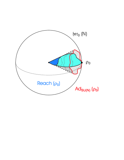
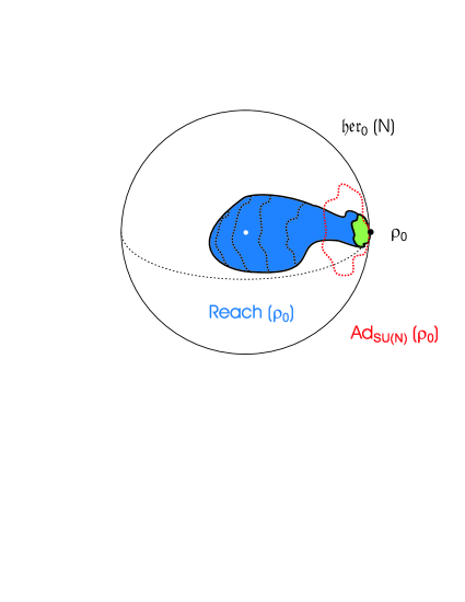
Abbildung 1: (Colour online) Quantum state-space manifolds for open relaxative systems shown as subsets of $\mathfrak{her}_{0}(N)$ with scales corresponding to the metric induced by the Hilbert-Schmidt scalar product. The centre of the high-dimensional sphere is the zero-matrix, and the geometry refers to larger systems, e.g., multi-qubit systems with $N\geq 4$. If in the absence of relaxation, the system is fully controllable, the reachable set for a fixed initial state represented as density operator $\rho_{0}$ takes the form of the entire unitary orbit $\operatorname{Ad}_{SU(N)}(\rho_{0})$. It serves as a reference and is shown as closed curve in red. In the text we focus on two different scenarios of open systems: (a) Dynamics of weakly Hamiltonian controllable systems with the Kossakowski-Lindblad term acting approximately as scalar $\Gamma_{L}\simeq\gamma{\rm 1\negthickspace l}{}$ are confined to the subset (marked in blue) of states evolving from $\rho_{0}$ under the action of the contraction semigroup $(0,1]\cdot\operatorname{Ad}_{SU(N)}$. The latter is depicted as grey surface of a ‘funnel’ intersecting the surface of the high-dimensional sphere in the unitary orbit. Towards the origin, i.e., at long times, the reachable set of wh-controllable systems typically wraps the entire surface (dark blue portion). (b) In the generic case when $[\Gamma_{L},H_{\nu}]\neq 0$ ($\nu=d;1,2,\dots,m$), the dynamics with initial state $\rho_{0}$ evolves within the volume shown in blue. New directions due to the interplay of coherent Hamiltonian evolution and relaxation make the dynamics explore a much larger state space than resulting from the simple contraction semigroup $(0,1]\cdot\operatorname{Ad}_{SU(N)}$, i.e. the surface in part (a) or even the volume contained in its interior. The intersection (green portion) of the volume $\operatorname{Reach}(\rho_{0})$ with the surface of the sphere consists of the set of all states reachable from $\rho_{0}$ in zero time or without relaxative loss. This may often collapse to the single point $\rho_{0}$ or its local unitary orbit Schulte-Herbrüggen et al. (2008b); Dirr et al. (2008).

Proposition III.2.

A unital open quantum system (19) with the Hamiltonian given by Eqn. (8) is

1. h-controllable, if $\mathfrak{k}_{c}=\mathfrak{su}(N)$ and no bounds on the control amplitutes $u_{j}$, $j=1,\dots,m$ are imposed;

2. wh-controllable, if $\mathfrak{k}_{d}=\mathfrak{su}(N)$ and $\Gamma_{L}\big{|}_{\mathfrak{her}_{0}(N)}\!=\!\gamma{\rm 1\negthickspace l}{}$ with $\gamma\geq 0$.

Moreover, for $U\in SU(N)$, the smallest $\lambda\in\mathbb{R}^{+}$ such that $\operatorname{Ad}_{U}\in\lambda\overline{\mathbf{P}}_{\Sigma}$ is given by ${\rm e}^{\gamma T^{*}(U)}$, where $T^{*}(U)$ denotes the optimal time to steer the lifted system given by Eqn. (20) without relaxation, i.e. for $\Gamma_{L}=0$, from the identity ${\rm 1\negthickspace l}{}$ to $\operatorname{Ad}_{U}$. In particular, for $\mathfrak{k}_{c}=\mathfrak{su}(N)$ one has $\lambda=1$ for all $U\in SU(N)$.

Proof. (a) First, suppose $\mathfrak{k}_{c}=\mathfrak{su}(N)$. Then, for $\Gamma_{L}=0$ the fact that we do not assume any bounds on the controls $u_{j}\in\mathbb{R}$ implies that one can steer from the identity ${\rm 1\negthickspace l}{}$ to any $\operatorname{Ad}_{U}$ arbitrarily fast. Thus for $\Gamma_{L}\neq 0$ a standard continuity argument from the theory of ordinary differential equations shows that one can approximate $\operatorname{Ad}_{U}$ up to any accuracy by elements of $\mathbf{P}_{\Sigma}$. Thus h-controllability holds.

(b) Suppose $\mathfrak{k}_{d}=\mathfrak{su}(N)$ and $\Gamma_{L}\big{|}_{\mathfrak{her}_{0}(N)}=\gamma{\rm 1\negthickspace l}{}$. By Corollary II.2, we obtain controllability of $\{\operatorname{Ad}_{U}\,|\,U\in SU(N)\}$ for $\Gamma_{L}=0$. Therefore, we can choose a control $u(t)$ which steers the identity ${\rm 1\negthickspace l}{}$ to $\operatorname{Ad}_{U}$ in optimal time $T^{*}(U)$. Applying the same control to the system under relaxation yields a trajectory which finally arrives at ${\rm e}^{-\gamma T^{*}(U)}\operatorname{Ad}_{U}$. Thus wh-controllability holds for $\lambda={\rm e}^{\gamma T^{*}(U)}$. Moreover, by the time optimality of $T^{*}(U)$ it is guaranteed that $\lambda={\rm e}^{\gamma T^{*}(U)}$ is the smallest $\lambda\in\mathbb{R}^{+}$ such that $\operatorname{Ad}_{U}\in\lambda\overline{\mathbf{P}}_{\Sigma}$ holds. $\blacksquare$

In general, an open quantum system that is fully controllable in the absence of relaxation will not be necessarily wh-controllable when including relaxation, even though it may be accessible. A counterexample showing this fact for the simplest two-level system and simulations will be provided in Kurniawan (to appear 2009). Establishing necessary and sufficient conditions for wh-controllability of open quantum systems is therefore an open research problem. For unital systems which are controllable in the absence of relaxation, we do expect that the ‘ratio’ of the Hamiltonian and the relaxative drift term completely determines wh-controllability. — Finally we will see that additional assumptions ensuring the preconditions of Theorem II.1 allow for inclusion of the global Lie wedge of Eqn. (19).

Theorem III.5.

Assume that the unital Master equation (19) with the Hamiltonian given by Eqn. (8) fulfills the following condition: there exists a pointed cone $\mathfrak{c}$ in the set of all positive semidefinite linear operators on $\mathfrak{her}_{0}(N)$ such that

1. $\Gamma_{L}\big{|}_{\mathfrak{her}_{0}(N)}\in\mathfrak{c}$ ;

2. $[\mathfrak{c},\mathfrak{c}]\subset\operatorname{ad}_{\mathfrak{su}(N)}$ and $[\mathfrak{c},\operatorname{ad}_{\mathfrak{su}(N)}]\subset\mathfrak{c}-\mathfrak{c}$ ;

3. $\operatorname{Ad}_{U}\mathfrak{c}\operatorname{Ad}_{U^{-1}}\subset\mathfrak{c}$ for all $U\in\mathrm{SU}(N)$ .

Then, the Lie subsemigroup $\overline{\mathbf{P}}_{\Sigma}$ of Eqn. (19) is contained in the Lie subsemigroup

$$\exp(-\mathfrak{c})\cdot\operatorname{Ad}_{SU(N)}$$

with Lie wedge $(-\mathfrak{c})\oplus\operatorname{ad}_{\mathfrak{su}(N)}$.

Proof. By Theorem II.5(b), it is sufficient to verify that $\exp(-\mathfrak{c})\cdot\operatorname{Ad}_{SU(N)}$ is a Lie subsemigroup with Lie wedge $(-\mathfrak{c})\oplus\operatorname{ad}_{\mathfrak{su}(N)}$. This will be achieved by applying Theorem II.1. To this end, we define $\mathfrak{g}:=\mathfrak{k}\oplus\mathfrak{p}$ with $\mathfrak{k}:=\operatorname{ad}_{\mathfrak{su}(N)}$ and $\mathfrak{p}:=(\mathfrak{c}-\mathfrak{c})+(\mathfrak{c}-\mathfrak{c})^{\top}$. Note that the set $\mathfrak{c}-\mathfrak{c}$ consisting of all differences within the cone $\mathfrak{c}$ coincides with the vector space spanned by $\mathfrak{c}$. Thus $\mathfrak{p}$ is a subspace of $\mathfrak{gl}(\mathfrak{her}_{0}(N))$ which is invariant under the involution $\Lambda\mapsto-\Lambda^{\top}$, where $\Lambda^{\top}$ denotes the adjoint operator of $\Lambda$ with respect to the Hilbert-Schmidt inner product on $\mathfrak{her}_{0}(N)$. Then, $\mathfrak{g}$ constitutes a Lie subalgebra of $\mathfrak{gl}(\mathfrak{her}_{0}(N))$ which is also invariant under the involution $\Lambda\mapsto-\Lambda^{\top}$. By choosing an orthogonal basis in $\mathfrak{her}_{0}(N)$, this invariance of $\mathfrak{g}$ translates into a matrix representation of $\mathfrak{g}$ which is stable under $X\mapsto-X^{\dagger}$. Then Proposition 1.59 in Knapp (2002) implies that $\mathfrak{g}$ is reductive and thus it decomposes into a direct sum of its centre $\mathfrak{z}$ and its semi-simple commutator ideal $\mathfrak{g}_{0}:=[\mathfrak{g},\mathfrak{g}]$, i.e. $\mathfrak{g}=\mathfrak{z}\oplus\mathfrak{g}_{0}$. Since $\operatorname{ad}_{\mathfrak{su}(N)}$, is contained in $\mathfrak{g}$, the centre $\mathfrak{z}$ is either trivial or $\mathbb{R}\cdot{\rm 1\negthickspace l}{}$. Thus, similar to Corollary 7.10 in Knapp (2002), one can show that $\mathbf{G}:=\langle\exp\mathfrak{g}\rangle$ is a closed connected subgroup of $GL(\mathfrak{her}_{0}(N))$. Therefore, Theorem II.1 applies to $\mathbf{G}$. In particular, $\mathfrak{k}$ and $\mathfrak{p}$ yield the required eigenspace decomposition of $\mathfrak{g}$. Hence we conclude that $\exp(-\mathfrak{c})\cdot\langle\exp\mathfrak{k}\rangle=\exp(-\mathfrak{c})\cdot\operatorname{Ad}_{SU(N)}$ is a Lie subsemigroup of $GL(\mathfrak{her}_{0}(N))$ with Lie wedge $(-\mathfrak{c})\oplus\operatorname{ad}_{\mathfrak{su}(N)}$. Thus the result follows. $\blacksquare$

The previous findings suggest the following procedure to compute or at least to approximate the Lie wedge of $\overline{\mathbf{P}}_{\Sigma}$:

1. Check, whether $\Gamma_{L}$ is self-adjoint (implying positive semidefiniteness for $\Gamma_{L}$). This is for example the case, if all $V_{k}$ in Eqn. (13) are Hermitian or, equivalently, if the Kossakowski-Lindblad term can be rewritten as a sum of double commutators, cf. Eqn. (22).

2. If (i) holds, find the smallest cone $\mathfrak{c}$ containing $\Gamma_{L}$ and satisfying the conditions of Theorem III.5.

Note that the above procedure yields but an outer approximation of the Lie wedge. In general, further arguments are necessary to obtain equality. For the generic two-level system in Altafini (2003), however, equality can be proven as the following result shows.

(a)                                                                             (b)                                                            
                   

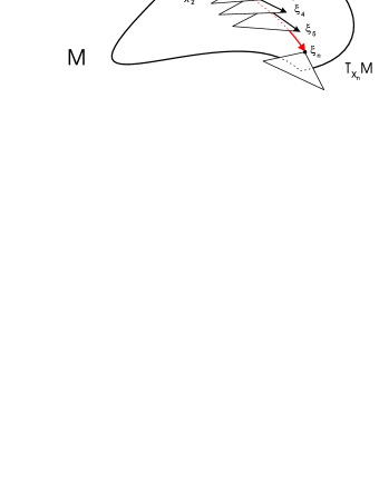
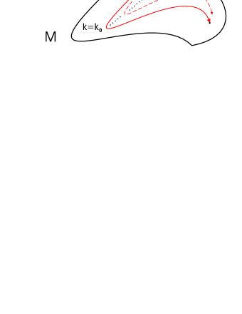
Abbildung 2: (Colour online) Steering dynamics of open relaxative systems represented by semigroup actions on a state space manifold $M$: (a) gradient-like method on the reachable set $\operatorname{Reach}(\rho)$ itself; admissible directions are confined to directions available in the Lie wedge; (b) optimal control approach as an ‘implicit method’ on the reachable set $\operatorname{Reach}(\rho)$ brought about by a gradient flow on the set of control amplitudes as in Fig. 3 of Ref. Schulte-Herbrüggen et al. (2008a). Note that in (b) the entire trajectory at all points in time is updated from $k\mapsto k+1$ thus exploring more directions than in (a), which may be an advantage over local gradient-like methods in open systems.

Corollary III.6.

Let $(\Sigma)$ be a unital h-controllable two-level system with generic Kossakowski-Lindblad term $\Gamma_{L}$. Then, the Lie subsemigroup $\overline{\mathbf{P}}_{\Sigma}$ coincides with

$$\overline{\mathbf{P}}_{\Sigma}=\exp(-\mathfrak{c})\cdot\operatorname{Ad}_{SU(2)}\subset{\mathbf{C}_{0}}\big{(}\mathfrak{her}_{0}(2)\big{)}$$

where $\mathfrak{c}$ denotes the convex cone

$$\mathfrak{c}:=\mathrm{conv}\big{\{}\lambda\Theta\Gamma_{L}\Theta^{\top}\;|\;\lambda\geq 0,\,\Theta\in\operatorname{Ad}_{SU(2)}\big{\}}$$ (24)

contained in the set of all positive semidefinite elements in $\mathfrak{gl}(\mathfrak{her}_{0}(2))$, cf. Remark III.1. Here, $\Theta^{\top}$ denotes the adjoint operator of $\Theta$ with respect to the Hilbert-Schmidt inner product on $\mathfrak{her}_{0}(2)$. Moreover, the Lie wedge of $\overline{\mathbf{P}}_{\Sigma}$ is given by $(-\mathfrak{c})\oplus\operatorname{ad}_{\mathfrak{su}(2)}$.

Proof. h-controllability of the system implies that $\operatorname{ad}_{\mathfrak{su}(2)}$ is contained in ${\rm L}(\overline{\mathbf{P}}_{\Sigma})$. Moreover, for $N=2$ it is known that $\Gamma_{L}\big{|}_{\mathfrak{her}_{0}(2)}$ is a positive semidefinite operator of $\mathfrak{gl}(\mathfrak{her}_{0}(2))$. Thus Theorem III.5 applied to the cone $\mathfrak{c}$ given by Eqn. (24) yields $\overline{\mathbf{P}}_{\Sigma}\subset\exp(-\mathfrak{c})\cdot\operatorname{Ad}_{SU(2)}$. For the converse inclusion, we refer to a standard convexity result on Lie saturated systems, cf. Jurdjevic (1997). $\blacksquare$

The geometry of reachability sets under contraction semigroups is illustrated and summerised in Fig. 1.

In general, it is quite intricate to show that outer approximations of the Lie wedge ${\rm L}(\overline{\mathbf{P}}_{\Sigma})$ derived from Theorem III.5 in fact coincide with ${\rm L}(\overline{\mathbf{P}}_{\Sigma})$. To the best of our knowledge, no efficient procedure to explicitly determine the global Lie wedge of Eqn. (14) does exist. Thus, for optimisation tasks on $\operatorname{Reach}(\rho)$, one currently has to resort to standard optimal control methods. A straightforward and robust algorithm is mentioned in the final section. Moreover, a new approach based on an approximation of ${\rm L}(\overline{\mathbf{P}}_{\Sigma})$ is sketched.

IV Relation to Optimisation Tasks

We follow Schulte-Herbrüggen et al. (2008a) in considering optimisation tasks that come in two scenarios, see also Fig. 2: (a) abstract optimisation over the reachable set and (b) optimal control of a dynamic system specified by its equation of motion (e.g. of Kossakowski-Lindblad form). More precisely, an abstract optimisation task means the problem of finding the global optimum of a given quality function $f$ over the reachable set of an initial state $\rho$ (independently of the controls that may drive the system to the desired optimum). In contrast, a problem is said to be a dynamic optimisation task if one is interested in an explicit (time dependent) ‘optimal’ control $u_{*}$ that steers the system as closely as possible to a desired final state, where ‘optimal’ can be time- or energy-optimal etc.

In cases where the reachable set $\operatorname{Reach}(\rho)$ can be characterised conveniently—as, for instance, in closed quantum systems where it is completely characterised by the system Lie algebra so that $\operatorname{Reach}(\rho)$ coincides with the system group orbit— numerical methods from non-linear optimisation (on manifolds) are appropriate to solve abstract optimisation tasks on $\operatorname{Reach}(\rho)$. Details have been elaborated in Schulte-Herbrüggen et al. (2008a). However, in open quantum systems a satisfactory characterisation of the reachable set $\operatorname{Reach}(\rho)$—e.g., via Lie algebraic methods—is currently an unsolved problem. Thus numerical methods designed for optimal control tasks (b) may serve as handy substitutes to solve also abstract optimisation tasks (a) on $\operatorname{Reach}(\rho)$.

To be more explicit, we consider the Kossakowski-Lindblad equation (19) with controlled Hamiltonian (8) in superoperator representation. We are faced with a system taking the form of a standard bilinear control system ($\Sigma$) for $\operatorname{vec}\rho\in\mathbb{C}^{N^{2}}$ reading

$$\operatorname{vec}\dot{\rho}=\big{(}A_{0}+\sum_{j=1}^{m}u_{j}A_{j}\big{)}\;\operatorname{vec}\rho$$ (25)

with drift term $A_{0}:=-{\rm i}({\rm 1\negthickspace l}{}_{N}\otimes H_{d}-H^{\top}_{d}\otimes{\rm 1\negthickspace l}{}_{N})-\widehat{\Gamma}_{L}$, control directions $A_{j}:=-{\rm i}({\rm 1\negthickspace l}{}_{N}\otimes H_{j}-H^{\top}_{j}\otimes{\rm 1\negthickspace l}{}_{N})$, and control amplitudes $u_{j}\in\mathbb{R}{}$, while $\widehat{\Gamma}_{L}$ is given by Eqn. (16). Then an optimal control task boils down to maximising a quality functional with respect to some finite dimensional function space, e.g., piecewise constant control amplitudes (for details see Schulte-Herbrüggen et al. (2008a) Overview Section). Clearly, one can reduce the size of system (25) by choosing a coherence-vector representation instead of a superoperator representation without changing the principle approach.

In this context, we would like to point out a remarkable interpretation of ${\rm L}(\overline{\mathbf{P}}_{\Sigma})$. The method just outlined may lead to a (discretised) unconstrained gradient flow on some high-dimensional $\mathbb{R}^{m}$. While the ‘local’ search directions (pulled back to state space) are confined to directions available in the ‘local’ Lie wedge of Eqn. (14), i.e. to the smallest Lie wedge generated by $A_{0}$ and $u_{j}A_{j}$, $u_{j}\in\mathbb{R}$, the entire method nevertheless allows to vary the final point $\rho(T)$ within an open neighbourhood of $\operatorname{Reach}(\rho)$, cf. Fig. 2(b). In contrast, a gradient-like method on the reachable set itself similar to the one for closed systems, but with search directions constrained to the (local) Lie wedge would in general fail, cf. Fig. 2(a).

Outlook: An Algorithm Exploiting the Lie-Wedge

Yet, combining both methods yields a new approach to abstract optimisation tasks: (i) First determine an inner approximation $\mathfrak{c}$ of the Lie wedge. (ii) Then, choose $n\in\mathbb{N}$ and define a map from the $n$-fold cartesian product $\mathfrak{c}\times\cdots\times\mathfrak{c}$ to $\mathbb{R}$ by $(\Omega_{1},\dots,\Omega_{n})\mapsto f({\rm e}^{\Omega_{n}}\cdots{\rm e}^{\Omega_{1}})$. Optimise this function over the convex set $\mathfrak{c}\times\cdots\times\mathfrak{c}$ and increase $n$ if necessary. We do expect that the performance of such an approach improves the better the approximation of the Lie wedge is. In particular, the length of the necessary products ${\rm e}^{\Omega_{n}}\cdots{\rm e}^{\Omega_{1}}$ will significantly decrease if $\mathfrak{c}$ is a good approximation to ${\rm L}(\overline{\mathbf{P}}_{\Sigma})$. Thus even for numerical aspects knowing the Lie wedge is of considerable interest. — With these remarks we will turn to other points pertinent in practice.

Practical Implications for Current Numerical Optimal Control

The above considerations have further implications for numerical approaches to optimal control of open systems in the sense of the dynamic task (b) of the previous section. They provide the framework to understand why time-optimal control makes sense in certain wh-controllable systems, whereas all other situations ask for explicitly taking the Kossakowski-Lindblad master equation into account. Consider three scenarios: (i) open quantum systems that wh-controllable with almost uniform decay rate, (ii) generic open systems with known Markovian (or non-Markovian) relaxation characteristics, and (iii) open systems with unknown relaxation behaviour.

In the simple case (i) of a wh-controllable system with almost uniform decay rate $\gamma$, $\Gamma_{L}$ approximately acts on $\mathfrak{her}_{0}(N)$ as scalar $\gamma{\rm 1\negthickspace l}{}$. Now assume that by numerical optimal control a build-up top curve $g(T)$ (value function) of maximum obtainable quality against total duration $T$ was calculated for the corresponding closed system with $\Gamma_{L}=0$. Moreover, let $T_{*}$ denote the smallest time allowing for a quality above a given error-correction threshold. Together with the uniform decay rate $\gamma$ this already provides all information if the quality function depends linearly on $\rho(T)$. Hence determining $T^{\prime}_{*}:=\operatorname{argmax}{}\{g(T)\cdot e^{-\gamma T}\}$ gives the optimal time for the desired solution. More coarsely if $T^{\prime}_{*}\simeq T_{*}$, time-optimal controls for the closed system are already a good guess for steering a wh-controllable system with almost uniform decay rate.

For case (ii), when the Kossakowski-Lindblad operator is known, but generically does not commute with all Hamiltonian drift and control components, it is currently most advantageous to use numerical optimal control techniques based on the Master equation with specific Kossakowski-Lindblad terms as has been illustrated in Schulte-Herbrüggen et al. (2006). The importance of including the Kossakowski-Lindblad terms roots in the fact that their non-commutative interplay with the Hamiltonian part actually introduces new directions in the semigroup dynamics. Likewise, in Rebentrost et al. (2006), we treated the optimal control task of open quantum systems in a non-Markovian case, where a qubit interacts in a non-Markovian way with a two-level-fluctuator, which in turn is dissipatively coupled to a bosonic bath in a Markovian way.

Clearly, the case of entirely unknown relaxation characteristics (iii), where e.g., model building and system identification of the relaxative part is precluded or too costly, is least expected to improve by suitable open-loop controls, if at all. Yet in Schulte-Herbrüggen et al. (2006) we have demonstrated that guesses of time-optimal control sequences (again obtained from the analogous closed system) may—by sheer serendipity—be apt to cope with relaxation. In practice, this comes at the cost of making sure a sufficiently large family of time-optimal controls is ultimately tested in the actual experiment for selecting among many optimal-control based candidates by trial and error. — Since this procedure is clearly highly unsatisfactory from a scientific viewpoint, efficient methods of determining pertinent decay parameters are highly desirable.

CONCLUSIONS

Optimising quality functions for open quantum dynamical processes as well as determining steerings in concrete experimental settings that actually achieve these optima is tantamount to exploiting and manipulating quantum effects in future technology.

To this end, we have recast the structure of completely positive trace-preserving maps describing the time evolution of open quantum systems in terms of Lie semigroups. On an abstract level, the semigroups of completely positive operators may thus be seen as a special instance within the more general theory of invariant cones Vinberg (1980); Hilgert et al. (1989). Here, we have identified the set of Kossakowski-Lindblad generators as Lie wedge: the tangent cone at the unity of the subsemigroup of all invertible, completely positive, and trace-preserving operators coincides with the set of Kossakowski-Lindblad operators.

In particular, (in the connected component of the unity) invertible quantum channels are time dependent Markovian, if they belong to the Lie semigroup generated by the Lie wedge of all Kossakowski-Lindblad operators. Moreover, a time dependent Markovian channel specialises to a time independent Markovian one, if the Lie wedge of an associated semigroup shows the stronger structure of a Lie semialgebra. — Likewise, in time dependently controlled open systems the existence of effective Liouvillians that comply with the dynamics given by the Master equation is linked to Lie-semialgebra structures.

In view of controlling open quantum systems, reachable sets have been described in the same framework. Compared to closed systems, the structure of reachable sets of open systems has turned out to be much more delicate. To this end, we have introduced the terms Hamiltonian controllability and weak Hamiltonian controllability replacing the standard notion of controllability, which fails in open quantum systems whenever the control restricts to the Hamiltonian part of the system. For simple cases, we have characterised Hamiltonian controllability and weak Hamiltonian controllability. These definitions also allow for characterising the conditons under which time-optimal controls derived for the associated closed systems already give good approximations in quantum systems that are actually open. In the generic case, however, obtaining optimal controls requires numerical tools from optimal control theory based on the full knowedge of the system’s parameters in terms of its Kossakowski-Lindblad master equation.

Finally, we have outlined a new algorithmic approach making explicit use of the Lie wedge of the open system. In cases simple enough to allow for a good approximation of their respective Lie wedges, a target quantum map can then be least-squares approximated by a product with comparatively few factors each taking the form of an exponential of some Lie-wedge element.

Since the theory of Lie semigroups has only scarcely been used for studying the dynamics of open quantum systems, the present work is also meant to structure and trigger further developments. E.g., the above considerations on $\mathfrak{k}$-$\mathfrak{p}$ decompositions may serve as a framework to describe the interplay of Hamiltonian coherent evolution and relaxative evolution: this interplay gives rise to new coherent effects. Some of them relate to well-established observations like, e.g., the Lamb-shift Lamb and Retherford (1947) or dynamic frequency shifts in magnetic resonance Abragam (1961); Werbelow (1979); Brüschweiler (1996), while others form the basis to very recent findings such as dephasing-assisted quantum transport in light-harvesting molecules Mohseni et al. (2008); Rebentrost et al. (2008a, b); Plenio and Huelga (2008); Caruso et al. (2009).