Diffusion-limited reactions and mortal random walkers in confined geometries

Abstract

Motivated by the diffusion-reaction kinetics on interstellar dust grains, we study a first-passage problem of mortal random walkers in a confined two-dimensional geometry. We provide an exact expression for the encounter probability of two walkers, which is evaluated in limiting cases and checked against extensive kinetic Monte Carlo simulations. We analyze the continuum limit which is approached very slowly, with corrections that vanish logarithmically with the lattice size. We then examine the influence of the shape of the lattice on the first-passage probability, where we focus on the aspect ratio dependence: Distorting the lattice always reduces the encounter probability of two walkers and can exhibit a crossover to the behavior of a genuinely one-dimensional random walk. The nature of this transition is also explained qualitatively.

1 Introduction

Random walks are ubiquitous in statistical physics as well as in the description of many natural phenomena. One key example is the study of diffusion-reaction systems.

In our particular case, one motivation for the following examination comes from a long-standing astrophysical puzzle, namely why there can be a large abundance of molecular hydrogen in interstellar clouds of gas and dust compared to the concentration of atomic hydrogen. For realistic conditions, the generally accepted mechanism is as follows Gould63 ; Hollenbach70 ; Hollenbach71 ; Hollenbach71a : Reactants impinge onto the surface of dust grains in a homogeneous fashion. They diffuse on the surface. Additionally, they desorb at a certain rate. If two such atoms meet during their traversal of the surface, they react to form a hydrogen molecule which immediately desorbs. We will sometimes refer to the recombination efficiency of such a system, defined as the fraction of impinging atoms that eventually react to yield a molecule.

To study the catalytic role of the dust grains in the astrophysically relevant regime of a small average number of atoms on the grain, one sets up a zero-dimensional master equation for the distribution of the number of reactants on a single grain, including terms for deposition, desorption and reaction, and solves for the stationary state of the system Green01 ; Biham02 . Rate equations for the mean adatom number do not suffice as they cannot account for crucial fluctuations and the non-Poissonian statistics of the reactant number that is induced by their confinement to a finite closed surface on which the reaction takes place Biham02 ; Lohmar06 . Within such a master equation treatment, apart from obvious single-atom rates, there only occurs a single two-particle parameter, viz. the sweeping rate describing how often a pair of atoms on the grain meets. One convenient way to express this parameter is by means of the encounter probability originally introduced in Krug03 in a continuum setting. This is the key quantity of a first-passage problem of two mortal random walkers: Mortality (i.e., terminating a random walk with a certain probability per step) corresponds to desorption of the atoms on the surface, the random walk to their diffusion, and the question (of first-passage nature) is whether the two walkers meet before either one dies, quantified by the encounter probability.

In general, a realistic full diffusion-reaction model has to be examined by microscopic Monte Carlo simulations (see e.g. Chang05 ). This is mostly owed to the fact that applications, and especially the astrophysical problem we described, call for the inclusion of disorder in the local rates of hopping and desorption, a feature hard to tackle analytically in more than one dimension. Despite the vast literature on diffusion properties in disordered media this even holds true (to the best of our knowledge) when we focus on the basic level of the encounter probability.

Still, it is useful to start with the analysis of simple homogeneous models that are accessible rather easily, both to establish a reference point for the validity of simulations and to make progress in the analytical exploration. On the level of the encounter probability this means we can employ results from the theory of homogeneous random walks. Furthermore, the discrete random walk model allows us to extend the generality step by step to different lattice types and shapes, hopefully providing deeper insight into the importance of these factors. Finally, it is expected that the problem will have some fundamental appeal for the theory of random walks in relation to reaction-diffusion systems in general.

Examples from seemingly remote fields to which this analysis might bear relevance include second-layer nucleation in epitaxial crystal growth Krug03 , chemical kinetics inside aerosol droplets Lushnikov03 , biophysical problems like exciton trapping on photosynthetic units Montroll69 and a range of search, transport and binding processes of or along DNA strands Slutsky03 ; Slutsky04 . Admittedly, in the latter case the homogeneous situation is only a first step to meaningful results, and the crucial two-dimensionality of our problem does not necessarily apply either.

Our goal in this paper is thus to further elucidate the meaning of the encounter probability, examining the pitfalls of the continuum limit to aid comparison to Monte Carlo simulations, and to analyze the influence of the lattice type and, most importantly, different geometries. We strive for a completely analytic theory to fully explain all findings of simulations. To this end, we will proceed as follows: Section 2 will first introduce the model and basic definitions along with our notation. We will then show how the fundamental quantity that we call ‘encounter probability’ can be obtained from a simple random walk calculation, and will analyze its asymptotic behavior. In Section 3 we investigate the subtle continuum limit which implies a logarithmically slow convergence to results obtained in a continuum model, which is crucial for comparison to simulations. We supplement this by simulation results in Section 4. Section 5 we extend the random walk calculations to a rectangular lattice to examine the role of the lattice shape, analyzing a quasi-one-dimensional limit and deriving and explaining the effect of a distorted aspect ratio. Finally, we present our conclusions.

2 Random walk treatment

2.1 Model and definitions

We consider a homogeneous two-dimensional lattice with periodic boundary conditions, meaning that all $S=L_{1}\cdot L_{2}$ sites are equivalent. Two walkers are randomly deposited on two (not necessarily different) sites of the lattice, then they move between nearest-neighbor sites with an undirected hopping rate $a$, and may desorb at a constant rate $W\ll a$. Whenever the two meet by one hopping onto the site occupied by the other (or by coinciding initial positions), they react and this random walk realization has ended successfully; the probability (averaged over random walk realizations and initial positions) at which this happens before either of the two walkers desorbs is called the encounter probability $p$ (subscripts will denote certain models and / or simulations from which it is obtained, as well as further specializations).

Here we will treat a discrete-time random walk, although a continuous-time version (CTRW) with an appropriate waiting time distribution might seem closer to the physical system at hand. We do this in order to keep the analytical treatment as simple as possible, and we will later argue and numerically prove (Section 4) that the discrete version accurately describes our situation. Due to homogeneity of the lattice, the problem in fact reduces to that of a single walker meeting a target site, cf. Appendix A.

2.2 Exact results

Quite generally, we are concerned with finite lattices translationally invariant in all directions, which extend to $L_{j}$ lattice sites in the $j$th of $d$ dimensions before periodically continuing. The exact expression of the random-walk encounter probability on such a lattice is re-derived in Appendix A and reads denHollander82

$$\begin{split}p_{\mathrm{rw}}^{-1}&=(1-\xi)SP^{*}(\vec{0};\xi)\\ &=\sum_{\vec{m}\in\Omega}\frac{1-\xi}{1-\xi\lambda(2\pi\mathbf{L}^{-1}\vec{m})}.\end{split}$$ (1)

Here,

$$\xi=1-\frac{W}{a+W}=\frac{a}{a+W}=\frac{1}{1+W/a}\lesssim 1$$ (2)

is the survival probability per step, $S=\prod_{j=1}^{d}L_{j}$ is the total number of sites, and $P^{*}(\vec{0};\xi)$ is the number of times a mortal walker on a periodic homogeneous lattice returns to the origin. $\Omega$ denotes the lattice, $\vec{m}$ is a ‘lattice vector’ of $d$ integer components $0\leq m_{j}\leq L_{j}-1$ with $j=1,\dots,d$, and $\mathbf{L}=\operatorname{diag}(L_{1},\dots,L_{d})$. Finally, $\lambda$ is the structure function (basically a discrete Fourier transform of the normalized transition probability) of the walk. We specify to $d=2$ at this point, where it reads $\lambda(\vec{k})=(\cos k_{1}+\cos k_{2})/2$ for an isotropic walk on a square lattice that we will further on label as being of ‘type (a)’, and $\lambda(\vec{k})=[\cos k_{1}+\cos k_{2}+\cos(k_{1}+k_{2})]/3$ for the isotropic walk on a triangular lattice (coordination number 6), now designated as ‘type (b)’.

We focus on the two-dimensional case with both lattice lengths much larger than unity and with ‘long survival’ defined by $1-\xi\ll 1$. The expression (1) then affords several regimes, characterized by the comparison of dimensionless ‘lengths’. Introducing the typical single-atom random walk length

$$\ell=\sqrt{a/W}=\sqrt{\frac{\xi}{1-\xi}}\gg 1$$ (3)

and with lattice dimensions $L_{1,2}\gg 1$, one can associate $1\ll\ell\ll L_{1,2}$ with ‘large’ lattices, and $1\ll L_{1,2}\ll\ell$ with ‘small’ lattices. The intermediate regime in which one lattice length is smaller, yet the other larger than the random walk length is to be discussed in a later Section.

For a still fairly large class of walks that includes the two cases (a) and (b), one summation in equation (1) can be carried out explicitly Montroll69 . Appendix B gives the result, which we generalized to include the case $L_{1}\neq L_{2}$. Whenever we need to numerically evaluate $p_{\mathrm{rw}}$ we use the resulting single-sum expression, further simplified for the two lattice types, and implemented in a small GNU Octave script.

The encounter probability as given above allows for the two random walkers to start on one site, and this counts as an encounter on the zeroth step. For applications and comparison to other models or simulations, we will often need to deal with the encounter probability $\tilde{p}_{\mathrm{rw}}$ calculated such that it only accounts for meeting of the walkers by hopping, and that does not allow the initial condition of walkers starting at the same site. The two quantities are related by

$$p_{\mathrm{rw}}=\frac{1}{S}+\left(1-\frac{1}{S}\right)\tilde{p}_{\mathrm{rw}},$$ (4)

as becomes obvious by splitting up $p_{\mathrm{rw}}$ according to the starting site of the second walker, i.e., either on the same site as the first one (with probability $1/S$), or on any other site (with probability $1-1/S$). This leads to the expression

$$\tilde{p}_{\mathrm{rw}}=\frac{Sp_{\mathrm{rw}}-1}{S-1}$$ (5)

in terms of $p_{\mathrm{rw}}$, and $\tilde{p}$ with other subscripts will henceforth denote probabilities $p$ that are obtained from other models using the corresponding analogous convention, i.e., excluding an encounter due to coinciding initial positions. In the context of hydrogen recombination on dust grain surfaces, the corresponding mechanism is the ‘Langmuir-Hinshelwood rejection’ of atoms that impinge on top of another; see e. g. Langmuir18 and references therein for early original work.

2.3 Large lattice approximation

Large lattices, formally given by $S\gg a/W\gg 1$ or, more precisely, by $1\ll\ell\ll L_{1,2}$, can equally well be defined as the regime in which boundary conditions, and (apart from the initial placement) the overall number of sites of the lattice no longer matter at all – even if the boundaries truly affected the random walker (say, by reflection), it either approaches the target or experiences the finiteness and (possibly) boundedness of the lattice, but never during one single walk. It is thus safe to simply send $L_{1,2}\to\infty$ in $P^{*}(\vec{0};\xi)$ in (1), by which procedure the sum becomes an area integral ($P(\vec{0};\xi)$ in the standard notation used in the Appendices). Some more details on the ensuing approximations are given in Appendix C, with the result that

$$p_{\mathrm{rw}}\approx\frac{a}{SW}\begin{cases}\pi\frac{1}{\ln[8a/W]}&\text{square lattice,}\\ \frac{2\pi}{\sqrt{3}}\frac{1}{\ln[12a/W]}&\text{triangular lattice,}\end{cases}$$ (6)

with relative errors of $\mathcal{O}(1-\xi)$.

2.4 Small lattice approximation

Here we have $1\ll L_{1,2}\ll\ell$ or $a/W\gg S\gg 1$. Again, we employ results for $P^{*}(\vec{0};\xi)$ from the random walk literature.

For the moment, we restrict ourselves to the case $L_{1}=L_{2}=\sqrt{S}$. The expansion for $1-\xi\ll S^{-1}\ll 1$ then reads

$$\begin{split}P^{*}(\vec{0};\xi)&=\frac{1}{S(1-\xi)}+c_{1}\ln(cS)\\ &\quad+\mathcal{O}\left(S^{-1},S(1-\xi),\sqrt{1-\xi})\right)\,,\end{split}$$ (7)

where $c$ and $c_{1}$ are real constants. This is shown in Montroll69 , also presenting the first calculations that deliver upon the important pre-factor inside the logarithm (for square and triangular lattices), which were extended and subject to minor corrections in denHollander82 (cf. the earlier and easily accessible derivation in Montroll65 , which unfortunately does not give this pre-factor). For the encounter probability one thus obtains

$$p_{\mathrm{rw}}\approx 1-\frac{SW}{a}c_{1}\ln(cS)\,.$$ (8)

It is important to note that the original expansion is valid in the regime $(1-\xi)S\pi^{-1}\ln(cS)\ll 1$, or equivalently, $1-p_{\mathrm{rw}}\ll 1$. This would thus be a more precise definition of a ‘small lattice’.

The constant $c_{1}$ has the value $1/\pi$ for the square lattice case (a), and $c_{1}=\sqrt{3}/(2\pi)$ for the triangular lattice (b), respectively. The crucial factor $c$ inside the logarithm appears in the different guise $c_{2}$ in Montroll69 , related to ours by $c_{2}/c_{1}=\ln c$. For the square lattice the ratio yields

$$\begin{split}\ln c&=\frac{\pi}{3}+2(\gamma-\ln\pi+\frac{1}{2}\ln 2)\\ &\quad+4\left[e^{-2\pi}+\frac{3}{2}e^{-4\pi}+\frac{4}{3}e^{-6\pi}+\dots\right]\\ &\approx 0.612807020\,,\end{split}$$ (9)

while for the triangular lattice this becomes

$$\begin{split}\ln c&=\frac{\pi}{2\sqrt{3}}+2(\gamma-\ln\pi+\frac{1}{2}\ln 3)\\ &\quad-4\left[e^{-\sqrt{3}\pi}-\frac{3}{2}e^{-2\sqrt{3}\pi}+\frac{4}{3}e^{-3\sqrt{3}\pi}-\dots\right]\\ &\approx 0.853262084\,,\end{split}$$ (10)

where we used standard rounding and checked the consistency of the numerical evaluation against the original figures and, when available, improved ones from denHollander82 . Here and in what follows, $\gamma\approx 0.5772156649$ denotes Euler’s constant.

3 Continuum limit

A natural question to ask is whether the model described above yields a reasonable continuum limit for $L_{1,2}\to\infty$; on the one hand, since such continuum limits are of genuine theoretical interest in themselves, on the other hand, since we have earlier solved a continuum model Lohmar06 to compare against. The answer will also provide important information for the comparison between analytical theory and simulations.

The proper scaling of the discrete random walk parameters then proceeds as follows. We want to stay in the same regime of the system, which means we need to keep both ratios $L_{j}/\ell$, and consequently $SW/a$, fixed. Further, we do not want to distort the given aspect ratio of the lattice, so that $L_{1}/L_{2}$ is kept constant as well (a moot point as long as we use quadratic lattices, i.e., $L_{1}\equiv L_{2}$ anyhow). With these constraints we let the number of adsorption sites become very large, $S\to\infty$. Such a joint limit preserves all quantities in our expressions that only depend on the ‘regime parameter’ $\sim S(1-\xi)$. The limiting behavior can thence be determined from the corresponding approximate results for the two regimes separately.

In the continuum (or “diffusion”) model proposed in Lohmar06 , a stationary diffusion equation for the probability density of a moving atom is solved on a spherical surface, and given an absorbing ‘target area’. The encounter probability is then calculated as the (suitably normalized) diffusion current entering this area. The results will be denoted by $p_{\mathrm{diff}}$.

We will also refer to results for $p$ obtained from random walk theory, however in a heuristic fashion Lohmar06 , using known expressions for $N_{\mathrm{dis}}$, the average number of distinct sites visited by a random walker after it has taken a given number of steps. The asymptotic result is that after $n\gg 1$ steps (on a two-dimensional regular lattice),

$$N_{\mathrm{dis}}\approx\frac{\pi n}{C\ln(Bn)}$$ (11)

with real positive constants $C$ and $B$ depending on the lattice type, viz. $C=1$ and $B=8$ for the square, and $C=\sqrt{3}/{2}$ and $B=12$ for a triangular lattice, respectively (see e.g. Hughes95 ). The encounter probability derived on this route will be labeled $p_{\mathrm{rw,heur}}$. Note that the above $N_{\mathrm{dis}}$ is the leading term of an asymptotic expansion, and thence a poor estimate for moderate values of $n$.

In the comparison of analytical results, we allow for walkers to meet by coinciding initial positions throughout, and we incorporate corresponding terms in the diffusion models as well; in short, we always use $p$ and not $\tilde{p}$.

3.1 Large lattices

The random walk result $p_{\mathrm{rw}}$ has been given above. Its diffusion model analogue reads

$$p_{\mathrm{diff}}\approx\frac{4ga}{SW}\frac{1}{\ln(4a/W)-2\gamma}\,,$$ (12)

where $g$ denotes a lattice-dependent factor; it is $g=\pi/4$ for the square lattice, and $g=\pi/(2\sqrt{3})$ for the triangular lattice, respectively. The heuristic result obtained from $N_{\mathrm{dis}}$ is

$$p_{\mathrm{rw,heur}}\approx\frac{\pi a}{CSW}\frac{1}{\ln(Ba/W)}\,,$$ (13)

with $B$, $C$ as defined above. Since comparison between the factors $g$ and $C$ immediately shows that for our cases $4g=\pi/C$, we see that not only the functional dependence, but also the numerical pre-factors of all three expressions $p_{\mathrm{rw}}$, $p_{\mathrm{diff}}$, and $p_{\mathrm{rw,heur}}$ coincide.

As far as the factor inside the logarithm is concerned, it is not too surprising that $p_{\mathrm{rw}}$ and $p_{\mathrm{rw,heur}}$ agree as well. However, the diffusion model expression $p_{\mathrm{diff}}$ clearly differs here, though this becomes irrelevant in the true limit $S\to\infty$. Note that there is no longer any imprint of the lattice type, as opposed to the discrete result. We should emphasize that in Lohmar06 care was taken that in the given form of the asymptotic expressions, all omitted terms are of higher order, particularly in the denominator expression, where further terms are of ‘polynomially’ smaller order than unity.

With this, the relative error of $p_{\mathrm{diff}}$ with respect to the random walk expressions can be calculated to yield

$$\Delta=\frac{\ln B-2(\ln 2-\gamma)}{\ln(a/W)+2(\ln 2-\gamma)}\,.$$ (14)

Since $2(\ln 2-\gamma)\approx 0.23$ and taking into account the values of $B$ this means that in the large lattice regime, the diffusion model encounter probability (and in its trail the sweeping rate and the recombination efficiency) systematically exceeds that given by the random walk result. The discrepancy vanishes in the continuum limit $S\to\infty$, however it only does so like $1/\ln(a/W)$ or as $1/\ln S$ (since $SW/a=\mathrm{const.}$).

3.2 Small lattices

The earlier results to compare the $p_{\mathrm{rw}}$ asymptotics against are as follows: For small lattices, we obtained the diffusion model expression

$$p_{\mathrm{diff}}\approx 1-\frac{SW}{4ga}\left[\ln(S/g)-1\right]\,,$$ (15)

with $g$ as defined in the previous Section. The heuristic random walk derivation yielded

$$p_{\mathrm{rw,heur}}\approx 1-\frac{CSW}{\pi a}\ln[BC/\pi\cdot S]\,.$$ (16)

Including the factor $c_{1}$ occurring in $p_{\mathrm{rw}}$ of (8) in the relation established between $g$ and $C$, we observe that it satisfies

$$c_{1}=\frac{1}{4g}=\frac{C}{\pi}.$$ (17)

Thus once again, the pre-factors as well as the functional dependence of all three expressions agree.

Turning to the pre-factor inside the logarithm, we have to resort to the numerical values of $\ln c$ as given in Section 2.4. Starting with the $p_{\mathrm{rw,heur}}$ expression, numerical evaluation of the corresponding $\ln BC/\pi$ yields numbers of $0.934711656$ and $1.196335728$ for type (a) and (b) lattices, respectively. While not in good agreement with the values for $\ln c$, this is still reasonable: Apart from the nature of the $N_{\mathrm{dis}}$ expansion, the ensuing heuristic derivation asserts that the walker does not die until it has traversed all $S$ sites, and includes inversion of the transcendental equation $N_{\mathrm{dis}}(t)=S$ which is approximated by one iteration. It is the very pre-factor just mentioned that suffers from this approximation. In contrast, the analogous factor in the diffusion model result reads $-\ln g-1$, and numerical evaluation provides $-0.758435525\dots$ and $-0.902276561\dots$ for types (a) and (b), respectively, both completely off.

For $S\to\infty$ with $SW/a=\mathrm{const.}$ we will eventually still leave the small lattice regime as $p$ drifts away from unity, cf. our earlier remark regarding the used expansion. To measure the error of the diffusion model, it is hence more appropriate to compare the complements $1-p$ of the two models, leading to a relative deviation

$$\Delta^{\prime}=-\frac{\ln(cg\operatorname{e})}{\ln(cS)}<0$$ (18)

of the diffusion model outcome relative to that of the random walk. Obviously, again the diffusion model delivers an encounter probability systematically larger than obtained from the random walk model, and again, this discrepancy vanishes only logarithmically with the system size $S\to\infty$.

3.3 Results

Besides the interest in the exact encounter probability of the random walk $p_{\mathrm{rw}}$ and its limiting behavior for the two regimes, we now have established that its asymptotics differ in logarithmic terms from that of the continuum model $p_{\mathrm{diff}}$. While the difference between discrete model results and those of the continuum model vanishes in the true continuum limit $S\to\infty$, $W/a\to\infty$ with $SW/a=\mathrm{const.}$, it does so only logarithmically in the system size $S$: This slow convergence is an inevitable direct consequence of the marginality of spatial dimension two for the random walk and diffusion, unfortunate for the comparison of discrete-space simulations to analytic results.

We finally plot (Figures 1 and 2) the relative discrepancy of the exact results of the diffusion model $p_{\mathrm{diff}}$ with respect to that of the random walk $p_{\mathrm{rw}}$ per cent, i.e., $100\cdot(p_{\mathrm{diff}}-p_{\mathrm{rw}})/p_{\mathrm{rw}}$ for the large lattice regime, substituted by the relative difference of the complements ($1-p$) for the small lattice plots. Inside a single plot, we sample lattice sizes determined by the lengths $L_{1}=L_{2}=L$ being the closest integers to give $S=4\cdot 10^{2},\,4\cdot 10^{3}\dots$, viz. $L=20$, $63$, $200$, $632$, $2000$, $6325$. Simultaneously, $\log(a/W)=2,\,3\dots$ increases with lattice size, such that the ‘regime’ parameter $SW/(4a)$ stays nearly constant and we properly approach the continuum limit. To compare, we also plot the error estimates $\Delta$ and $\Delta^{\prime}$ as appropriate for the given regime.

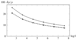
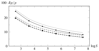
Figure 1: Relative difference (in percent) of $1-p_{\mathrm{diff}}$ w.r.t. $1-p_{\mathrm{rw}}$ for $SW/(4a)=10^{-3}$ (top) and $SW/(4a)=10^{-2}$ (bottom, still a small lattice), type (a) (dashed / squares), type (b) (dotted / triangles); thinner lines the prediction $-\Delta^{\prime}$.

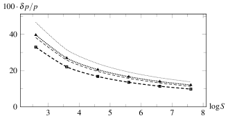
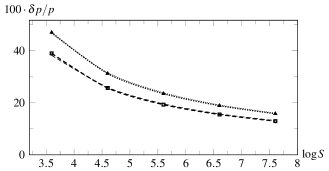
Figure 2: Relative difference (in percent) of $p_{\mathrm{diff}}$ w.r.t. $p_{\mathrm{rw}}$ for $SW/(4a)=10^{0}$ (top, already a large lattice) and $SW/(4a)=10^{1}$ (bottom), type (a) (dashed / squares), type (b) (dotted / triangles); thinner lines the prediction $\Delta$.

In both regimes the error predictions nicely agree with the discrepancy of the exact results, with increasing precision the further we go into a certain regime. This also verifies that the asymptotic results used to derive the estimates are correct, and that the discrepancy is not due to any relevant terms erroneously omitted. The error generally shows the predicted slow logarithmic decrease in the system size. Moreover, one can clearly see that it is considerable for all lattices, even for the largest ones, and the error even increases the further we enter one regime.

4 Simulations

We already mentioned that in many applications, the full microscopic kinetics is simulated within the Monte Carlo approach. Thence here we quantitatively compare our analytic predictions for the encounter probability to the corresponding simulation results. It is fairly easy to simulate both, the stochastic two-particle system for which we defined the encounter probability $p$, but also the ‘full’ diffusion-reaction system including continuous stochastic deposition of new random walkers, yielding results for the recombination efficiency of this process.

We use a standard kinetic Monte Carlo algorithm to keep track of individual atoms deposited onto, hopping around on and desorbing from the lattice. As in the random walk description, the lattice is homogeneous, with periodic boundaries. All waiting times for events are stochastically distributed according to an exponential distribution with the average waiting time given by the inverse rate of the corresponding process. In the simplified case of the two-particle simulation we consider two independently moving and desorbing atoms in continuous time – though with an arbitrarily rescaled time step permitted by the homogeneous environment. This is the simplest implementation of the continuous-time random walk (CTRW) introduced by Montroll65 .

The algorithm respects the Langmuir-Hinshelwood rejection described earlier, i.e., atoms impinging on top of occupied sites are repelled. Hence for faithful comparison between simulation and random walk theory, in this whole Section we will refer to $\tilde{p}_{\mathrm{rw}}$ instead of $p_{\mathrm{rw}}$.

Let us first relate what follows to earlier work. The simulation of a single moving (and possibly desorbing) atom that is to meet a fixed immortal target site in a homogeneous environment (hence the situation used in deriving $p_{\mathrm{rw}}$) obviously obliterates any notion of continuous time and can be fully described in terms of steps of the walk. It is therefore a truism that any correctly working microscopic Monte Carlo simulation of such a system has to converge to $p_{\mathrm{rw}}$ if we sample enough individual trials. For the case without desorption (where the interest is not in the probability of an encounter, but rather in the statistics of the number of steps this takes), the predictions of Montroll69 have been confirmed by Monte Carlo simulations in Hatlee80 , where the effect of alternative boundary conditions of the finite lattice is also examined.

Now if both reactants can move and desorb, it makes sense to simulate them in continuous time to let all events happen in an ordered fashion, and this is what we have done in all simulations we refer to herein. The equivalence of both scenarios (two walkers vs. one walker, and regarding the encounter probability) was clear in the stationary diffusion model, due to its continuum nature, the absence of any time, and its dealing with a “concentration” that is obtained by averaging over random walk realizations. For the single instance of the CTRW we note that (in our homogeneous setting) we can still treat one of the two walkers as fixed: If it is to make a move, we may simply re-label lattice sites accordingly and let the other walker perform an appropriate step instead. If it dies, the trial is ended as well as if the other walker had died. Hence the system can equally be described as a single walker that is to meet a target site, hopping and dying at twice the rates of each of the two original random walks, and still with exponentially distributed waiting times. This change of rates does not alter the survival probability per step and thence does not change the encounter probability. Moreover, while the number of steps performed in a given time is a stochastic quantity for the CTRW (as opposed to the discrete-time random walk, their relation for a huge class of waiting time distributions examined in e. g. Bedeaux71 ), the time passed never matters for the encounter probability, so that a description in terms of steps only is fully justified.

Indeed, we can report excellent agreement of the encounter probability $\tilde{p}_{\mathrm{rw}}$ obtained from the random walk model with that found in Monte Carlo simulations, $\tilde{p}_{\mathrm{mc}}$, see Appendix D for details. This holds for arbitrary parameters $S$ and $W/a$, as well as for both types of lattice, and gives credence to the correctness of our simulation method.

To obtain $\tilde{p}_{\mathrm{mc}}$ we sampled $N=10^{6}$ individual trials (except for the largest $S$ and $\ell$, where we chose $N=10^{5}$ due to time constraints) of the Monte Carlo simulation of two atoms moving in continuous time. Such a repeated sampling of independent Bernoulli trials with (unknown) exact success probability $p$ (corresponding to recombination in our context) yields an absolute standard deviation of the outcome of $\sigma=\sqrt{p(1-p)/N}$. Thus $\tilde{\sigma}=\sigma/p$, evaluated using the (known) values for $\tilde{p}_{\mathrm{rw}}$, is the expected relative standard deviation for simulations. Obviously $\tilde{\sigma}$ becomes fairly large for small $p$, i.e., approaching the large lattice regime.

The binomial distribution for the number of recombinations with fixed success probability $p$ of the individual trial and for the number of samples $N\to\infty$ tends to a Gaussian distribution, so the distribution for the numerically found $\tilde{p}_{\mathrm{mc}}$ should tend to a normal distribution with the above standard deviation. Roughly a third of all results are then expected to lie outside a corridor of half width $\tilde{\sigma}$ due to fluctuations; counted over all simulation data points for the quadratic lattices we find precisely $26/78$ values outside this range. The largest deviations from $\tilde{p}_{\mathrm{rw}}$ are of the order of less than $3\tilde{\sigma}$, with the largest absolute deviations smaller than $7\%$. Furthermore there is no systematic over- or underestimate of the theory. Similar results were obtained for rectangular lattices (see Appendix D). We conclude that the simple random walk result describes the continuous-time simulations to excellent accuracy. On a side note, this shows that the diffusion model results would completely fail to describe simulation results, most pronounced in the large lattice regime.

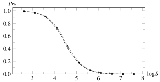
Figure 3: Random walk encounter probability $p_{\mathrm{rw}}$ as a function of the (logarithmic) grain size for $W/a=10^{-5}$, and for a type (a) (dashed / squares) or a type (b) (dotted / triangles) lattice, respectively.

The excellent agreement between simulations and random walk theory allows us to revisit the effect of the lattice type on the recombination efficiency, which was discussed in Lohmar06 with reference to the Monte Carlo simulations reported in Chang05 . We have seen above in Section 3 that, to leading order, the lattice type enters the encounter probability through the multiplicative constant (17), which differs by about $15\%$ between the square and triangular lattices. The effect obtained using the full, exact expression for $p_{\mathrm{rw}}$ is of the same order or smaller, as illustrated in Figure 3. Since neither the sweeping rate $A$ nor the recombination efficiency depend more strongly on the lattice type than $p$ itself Lohmar06 , we may conclude that significant lattice type effects cannot be expected in simulations that faithfully represent the reaction-diffusion model treated in this paper. The discrepancy with the results of Chang05 , where efficiencies on square and triangular lattices were found to differ by a factor of 2, thus remains.

5 Shape of the lattice

As was mentioned in Lohmar06 ; Krug03 , the diffusion model results for the encounter probability can be compared to those obtained in a completely analogous way for a flat disc with a reflecting outer boundary and a fixed absorbing target in its center. A detailed analysis (again also accounting for encounters “by deposition”) shows that upon natural identification of the parameters, in both regimes the functional form and pre-factors coincide, but while in the “large-disc” regime the asymptotics reproduces the sphere result (12) exactly including the logarithmic factor (or coequal $\mathcal{O}(1)$ terms), it slightly differs in the “small-disc” regime, where

$$p_{\mathrm{diff,disc}}\approx 1-\frac{SW}{4ga}\left[\ln(S/g)-3/2\right]\,,$$ (19)

with the lattice factor $g$ defined before. Numerical evaluation shows that there is only a small (of the order of a few percent) difference of both models in between these limiting cases.

This re-assures our conviction that curvature effects should not matter with $S\gg 1$: The basic reason is that the radius of curvature (in units of lattice spacing) is of the order of the system size. The absence of any effect is obvious for the large-lattice regime, when a random walk typically does not travel a distance long enough to feel the radius of curvature, $\ell\ll\sqrt{S}$. But as soon as $\ell\sim\sqrt{S}$, nearly the whole lattice is swept by the walk anyway, the small fraction not explored not depending on curvature, but on the failure of locally dense exploration.

Note that the difference of the logarithmic factors of sphere and disc in the small-lattice regime appears in the same order of magnitude as the discrepancy between lattice and continuum models in Section 3, although the former models (in contrast to the latter ones) substantially differ in topology and boundary conditions. While at some point we had considered curvature and connectivity effects responsible for the discrepancy between the diffusion model result and that obtained for the random walk, this comparison strongly (and quantitatively) suggested otherwise.

It is clear, however, that boundary conditions and the general shape of the lattice should have some effect on the random walk properties (at least in certain parameter regimes), and possibly on the encounter probability $p$. Related questions concerning the importance of confined geometries, without desorption and correspondingly focusing on mean first-passage times instead of first-passage probabilities, have been examined in detail in a recent remarkable series of papers Condamin05 ; Condamin06 ; Condamin07 . Moreover, as we have seen, the peculiarities of spatial dimension two are very important for the features of $p$ – what happens then, is one naturally ensuing question, if we distort the lattice shape in such a way that it becomes effectively one-dimensional?

In view of the line of thought of this article we focus here on the analysis of a torus lattice (periodic and rectangular) with distorted aspect ratio, that is, with different lengths $L_{1}$ and $L_{2}$ in the two directions. We will refer to the case $L_{1}\neq L_{2}$ as rectangular, while we call $L_{1}=L_{2}$ a quadratic lattice, the latter not to be mixed up with the term square that we use exclusively to label a certain lattice type (i.e., its internal structure) as opposed to its shape or geometry.

Let us therefore refine our notion of small and large lattice regimes. We still assume all three lengths $L_{1}$, $L_{2}$, $\ell\gg 1$ throughout. Without any loss of generality, let $L_{2}\leq L_{1}$, but we might further specialize to $L_{2}\ll L_{1}$. Ordering lengths, we are then left with three (instead of our former two) asymptotic regimes defined by the ordering of length scales:

• $1\ll\ell\ll L_{2}\leq L_{1}$.

• $1\ll L_{2}\ll\ell\ll L_{1}$.

• $1\ll L_{2}\leq L_{1}\ll\ell$.

The first case corresponds to the earlier large-lattice regime; the third case to small lattices. The intermediate regime in which the walk easily sweeps one dimension but is typically short compared to the other is a new property. We define the aspect ratio as $\mu:=L_{2}/L_{1}\in(0,1]$.

We will dismiss the large-lattice case for most of the sequel. In this regime, boundaries are effectively not felt by the random walker, and the appropriate double integral limit of (1) yields a result that only depends on the total number of sites $S$ (and no longer on $L_{1,2}$), as given in Section 2.3.

5.1 Overall behavior

We keep $S$ and $\xi$ constant and show the encounter probability $p_{\mathrm{rw}}$ on a type (a) square lattice as a function of (the logarithm of) the aspect ratio $\mu$ for both, one absolutely small ($S=4\times 10^{2}$) and one absolutely large lattice ($S=4\times 10^{6}$). In Figure 4, we start in the small-lattice regime for the quadratic case (rightmost in the plot), whereas Figure 5 starts in the large-lattice regime. There is no qualitative difference between the two lattice types with respect to any plot.

Figure 4: Encounter probability (on a square lattice) as a function of $\log\mu$, for fixed sizes $S=4\times 10^{6}$ (thick) and $S=4\times 10^{2}$ (thin), respectively, and $SW/(4a)=10^{-2}$ in both cases.

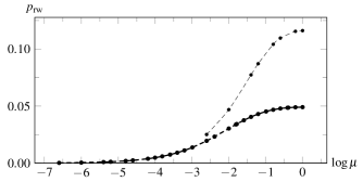
Figure 5: As Figure 4 with $SW/(4a)=1$.

In all cases the encounter probability shows a strong monotonic decline upon distortion (i.e., moving left in the Figures), though with a less pronounced shape and ending at a fair fraction of its peak value for the absolutely small lattice. We will first analyze several aspects of this transition, finally putting our findings together in a qualitative explanation.

5.2 Extreme distortion

We start with a simple observation. First, let us use the two-dimensional result for $p_{\mathrm{rw}}$ on a type (a) square lattice, and let one lattice dimension shrink to one lattice unit only ($S=L_{1}L_{2}=L\cdot 1$). What we get from (1) is

$$p_{\mathrm{rw}}^{-1}=\sum_{m=0}^{S-1}\frac{1-\xi}{1-(\xi/2)\left(\cos(2\pi m/S)+1\right)}\,,$$ (20)

where we have not yet used any summation results. Second, we immediately start with a genuine one-dimensional lattice, and then the sum for an unbiased walk (different structure function!) reads

$$p_{\mathrm{rw,\,1d}}^{-1}=\sum_{m=0}^{S-1}\frac{1-\xi}{1-\xi\cos(2\pi m/S)}\,,$$ (21)

which is obviously different from the former limit. We see that $p_{\mathrm{rw,\,1d}}>p_{\mathrm{rw}}$ for equal number of adsorption sites $S$ and equal $\xi$.

The explanation of this result of an “extremely distorted” situation provides some insight for the general problem. In the two-dimensional version, the walker still performs steps in the direction in which there is only one lattice unit length (of the periodic lattice), and one can imagine it as walking around on a very ‘thin’ torus with one dimension completely “wrapped up”. Contrary to this, the truly one-dimensional walk only performs steps in the direction in which the lattice is extended. The net effect is that the two-dimensional walker wastes on average half the number of steps it takes by walking in the ‘wrong’ dimension and not coming any closer to the target site. In fact, this suffices to re-gain one result from the other heuristically: The 2d-walk corresponds to a 1d-walk with the same desorption rate $W$, but with the undirected hopping rate effectively halved by the useless waiting steps, $a\to a/2$. This change translates to $(1-\xi)/\xi\to 2(1-\xi)/\xi$, and minimal manipulation of the two expressions given above shows that this casts the 1d-walk result into that for the two-dimensional walk (see Montroll73 for a related discussion).

5.3 Small lattices and $L_{1}\neq L_{2}$

For the following analysis, we generalized the asymptotic result for $P^{*}(\vec{0};\xi)$ of Montroll69 ; denHollander82 to the case $L_{1}\neq L_{2}$, at least in the vicinity of the square lattice. To this end, one mainly has to diligently separate the different $L_{j}$s in the derivation and to check that the individual steps continue to hold. Based on the generalized exact expressions given in Appendix B, we obtain

$$\begin{split}&\qquad P^{*}(\vec{0};\xi)=\frac{1}{L_{1}L_{2}(1-\xi)}+\frac{\ln L_{1}}{r\pi(1-2q_{0})}\\ &+\frac{\frac{L_{2}}{3L_{1}}+\frac{1}{r\pi}[2\gamma+2\ln(2/\pi)-\ln(1+\eta)]+S_{3}^{(0)}/r}{2(1-2q_{0})}\\ &+\frac{-\frac{1}{3}+\frac{(3\eta-1)\pi}{36r}\frac{L_{2}}{L_{1}}+S_{3}^{(1)}/r}{2(1-2q_{0})L_{1}L_{2}}\\ &+\mathcal{O}(L^{-4})+\mathcal{O}(1-\xi)^{1/2},\end{split}$$ (22)

where, first of all, terms are arranged in orders of $\sqrt{1-\xi}$, as this is the smallest quantity, and, inside, according to orders of $L_{1,2}$. The parameter $q_{0}$ is the probability a step is directed into a particular lattice unit direction, $q_{1}$ and $q_{2}$ denote transition probabilities into the diagonal directions, cf. Appendix B. Furthermore, we adopted the definitions

$$r =\frac{2[(q_{0}+2q_{1})(q_{0}+2q_{2})]^{1/2}}{1-2q_{0}}\,$$ (23)

$$\eta =\frac{q_{0}(1-2q_{0})}{(q_{0}+2q_{1})(q_{0}+2q_{2})}-1\,,$$

which take the values $r=1=\eta$ for the square lattice case (a), and $r=\sqrt{3}/2$, $\eta=1/3$ for the triangular lattice case (b). The only parts in the above expression that have to be explicitly evaluated for the two lattice types are the sum contributions $S_{3}^{(0,1)}$. Unfortunately, their generalization to $L_{1}\neq L_{2}$ is reasonably feasible only for the square lattice case (a), on which we now focus and where

$$S_{3}^{(0)} =\frac{4}{\pi}\Bigl{(}\operatorname{e}^{-2\pi L_{2}/L_{1}}+\frac{3}{2}\operatorname{e}^{-4\pi L_{2}/L_{1}}+\frac{4}{3}\operatorname{e}^{-6\pi L_{2}/L_{1}}+\dots\Bigr{)},$$ (24)

$$S_{3}^{(1)} =-\frac{4\pi}{3}\left(\frac{L_{2}}{L_{1}}\right)\Bigl{(}\operatorname{e}^{-2\pi L_{2}/L_{1}}+3\operatorname{e}^{-4\pi L_{2}/L_{1}}$$

$$\qquad+4\operatorname{e}^{-6\pi L_{2}/L_{1}}+\dots\Bigr{)}$$

$$\quad+\frac{8\pi^{2}}{3}\left(\frac{L_{2}}{L_{1}}\right)^{2}\Bigl{(}\operatorname{e}^{-2\pi L_{2}/L_{1}}+6\operatorname{e}^{-4\pi L_{2}/L_{1}}$$

$$\qquad+12\operatorname{e}^{-6\pi L_{2}/L_{1}}+\dots\Bigr{)}.$$

Due to the nature of the involved approximations, the expansion is asymmetric in the lattice lengths. In the form given above, $L_{2}$ is the limit of the ‘inner’ sum that is explicitly and exactly evaluated (see Appendix B), while the other length $L_{1}$ appears as the upper limit in several Euler-MacLaurin formulae in the derivation. Therefore we expected the result would fit best for the case where $L_{2}\leq L_{1}$. This is the ordering we will consistently assume throughout the following.

The detailed assumptions on the length scales that enter the result are as follows: First, we need $L_{1}L_{2}(1-\xi)\ll 1$ for the general form of the $P^{*}$ expansion to be meaningful, cf. Montroll69 , Eq. B35. Further, the result relies on the fact that the dimension for which the sum is explicitly evaluated is small, $L_{2}\ll\ell=\sqrt{\xi/(1-\xi)}\approx 1/\sqrt{1-\xi}$, necessary for the used expansion of the first summand to converge (ibid. Eqs. B11, B12), while the other is absolutely large $L_{1}\gg 1$ (for applicability of the Euler-MacLaurin formula). Lastly, $L_{2}/L_{1}$ must not be too small (owed to convergence in Eqs. B28 ff. ibid., also see (24)). This set of conditions applies to the small-lattice regime whenever $L_{2}/L_{1}$ does not become too small; but it is also satisfied for the intermediate regime provided that additionally, $L_{1}L_{2}(1-\xi)\ll 1$.

It is fairly obvious that under certain conditions we may exchange the role of the lengths $L_{2}<L_{1}$ in the derivation, such that the summation is carried out for the larger length $L_{1}$ instead. Thence the results (22) and (24) will remain valid upon swapping all occurrences of $L_{1}$ and $L_{2}$ if the aforementioned conditions remain satisfied; we refer to this as the ‘swapped-lengths’ version. As then, $L_{1}\ll\ell$ is necessary, we are restricted to the small-lattice regime; the remaining condition is equivalent to $L_{1}/L_{2}^{3}\ll 1$, as follows from careful inspection of the B28 derivation of Montroll69 .

A consistency check between the result as it reads above and the swapped-lengths version has to take into account that it can only hold in the small-lattice regime, and that the orders of several terms change. Numerical comparison of both versions and comparisons with the evaluation of the exact result $p_{\mathrm{rw}}$ show that, indeed, the swapped-lengths version reproduces the exact result more accurately than the form given above, as it circumvents the aforementioned convergence issue. This is only a minute problem however, and both versions agree and are in good agreement with the exact result (for the square lattice) over a certain range of distortions (checked for $\mu=L_{2}/L_{1}=1/4\dots 1$ for the small-lattice regime with $S=4\cdot 10^{6}$, $a/W=10^{8}$, the agreement of the swapped-lengths version with the exact result extending farther down to $\mu\sim 1/10$).

5.4 Small distortion

We now want to approach the question of the aspect ratio influence not from the extreme case, but in contrast starting to deform a quadratic lattice. Concretely, we ask when (and to what effect) the random walk feels the global change if we slightly distort a quadratic lattice of $S=L^{2}$ sites, keeping $W/a$ and $S$ fixed. The latter condition is necessary since (judging from previous results) the effect of varying $S$ is dominant otherwise; this hinders us from simply distorting the lattice lengths to “nearby” integer dimensions ($(L-1)(L+1)=S-1$).

Therefore we proceed as follows: We treat $p_{\mathrm{rw}}$ as a function $p_{\mathrm{rw}}(\mu,S,\xi)$, keep the latter two arguments fixed, and assume that the aspect ratio $\mu$ can be varied continuously. Any statements about the local behavior of that function around the quadratic shape value $\mu^{*}$ remain sensible as long as higher-order terms do not restrict their validity to intervals too small. We do not believe this to be the case, basically because we cannot conceive of any mechanism that could render the behavior of $\left.p_{\mathrm{rw}}\right\rvert_{S,\,\xi=\mathrm{const},\,\mu\leq\mu^{*}}$ non-monotonic.

The effect of a small distortion could depend on the regime we are in. We now focus on the small-lattice regime, since we expect aspect ratio effects to be most prominent there, and since for this case, we could obtain the general asymptotic behavior in Section 5.3. Note that starting from a square lattice with the question at hand rules out the intermediate regime, and that of large lattices was argued not to be of much interest above.

Now $\operatorname{d}\!^{2}p/\operatorname{d}\!\mu^{2}=[S(1-\xi)]^{-1}\frac{\operatorname{d}\!^{2}(P^{*}(\vec{0};\xi))^{-1}}{\operatorname{d}\!\mu^{2}}$, and at the extremal point, $\frac{\operatorname{d}\!^{2}(P^{*}(\vec{0};\xi))^{-1}}{\operatorname{d}\!\mu^{2}}=-(P^{*}(\vec{0};\xi))^{-2}\frac{\operatorname{d}\!^{2}P^{*}(\vec{0};\xi)}{\operatorname{d}\!\mu^{2}}$, since the first derivative vanishes ($\left.\operatorname{d}\!p/\operatorname{d}\!\mu\right\rvert_{\mu=\mu^{*}}=0$ due to $L_{1}\leftrightarrow L_{2}$ symmetry of $p$). For our purposes we only need to find the sign of the second $P^{*}(\vec{0};\xi)$ derivative. To this end, we use the approximation of Section 5.3, supposing that the dominant contributions to $P^{*}(\vec{0};\xi)$ are also dominating the sign of the second derivative. As a function of $\mu$, (22) reads

$$\begin{split}P^{*}(\vec{0};\xi)&=\mathrm{const}+\frac{\ln\sqrt{S/\mu}}{r\pi(1-2q_{0})}+\frac{\mu/3+S_{3}^{(0)}/r}{2(1-2q_{0})}\\ &+\frac{\frac{(3\eta-1)\pi}{36r}\mu+S_{3}^{(1)}/r}{2(1-2q_{0})S}+\mathcal{O}\left(L^{-4},(1-\xi)^{1/2}\right),\end{split}$$ (25)

and therefore in the second derivative, only the $S_{3}$ contributions and those from the square root term remain, viz.

$$\frac{\operatorname{d}\!^{2}P^{*}(\vec{0};\xi)}{\operatorname{d}\!\mu^{2}}\approx\frac{\frac{1}{\pi}\mu^{-2}+\operatorname{d}\!^{2}(S_{3}^{(0)}+S_{3}^{(1)}/S)/\operatorname{d}\!\mu^{2}}{2r(1-2q_{0})}\,.$$ (26)

The $S_{3}^{(1)}$ contribution is irrelevant due to the $S^{-1}$ factor, and

$$\begin{split}\frac{\operatorname{d}\!^{2}S_{3}^{(0)}}{\operatorname{d}\!\mu^{2}}&=16\pi\Bigl{(}\operatorname{e}^{-2\pi\mu}+6\operatorname{e}^{-4\pi\mu}+12\operatorname{e}^{-6\pi\mu}+\dots\Bigr{)}\,,\end{split}$$ (27)

where (as before), we only treat case (a) with $r=1=\eta$. Numerical evaluation of this term at $\mu=1$ yields approximately $0.095$. Thence, $\frac{\operatorname{d}\!^{2}P^{*}(\vec{0};\xi)}{\operatorname{d}\!\mu^{2}}>0$, and consequently, $\operatorname{d}\!^{2}p/\operatorname{d}\!\mu^{2}<0$: the encounter probability of the random walk in the small-lattice regime has a maximum for the quadratic lattice, and it decreases with any distortion from this shape. This is the quantitative foundation of our heuristic arguments in Section 5.6.

5.5 The quasi-one-dimensional limit

Finally we want to clarify the nature of the transition to effective one-dimensionality: What happens if the aspect ratio goes to infinity, so that the macroscopic structure of the lattice becomes quasi-one-dimensional?

First, we comment on the relationship between the regimes of the one-dimensional and the distorted two-dimensional lattices. In the 2d-large-lattice regime, $\ell$ is the smallest length scale; this cannot be sensibly related to any one-dimensional situation. It is then clear that the large-lattice regime on a one-dimensional lattice of length $L\gg\ell_{\mathrm{1d}}$ corresponds to the intermediate regime of the two-dimensional situation, i.e., $1\ll L_{2}\ll\ell\ll L_{1}$, the common feature being that exactly one lattice dimension is much larger than the typical random walk. The remaining small-lattice regime of the two-dimensional case ($1\ll L_{2}\ll L_{1}\ll\ell$) has its analogon in the small-lattice regime $1\ll L\ll\ell$ of the one-dimensional case, in both cases defined by a diffusion length that exceeds any lattice dimension.

We now consider a scaling limit of the three lengths in the (two-dimensional) small-lattice regime so that we can apply the result of Section 5.3. Since $\ell$ is the largest length, we use $\ell\to\infty$ as the basic scale in powers of which we express the $L_{i}$ behavior. In the original form (22), $L_{2}/L_{1}\to 0$ is not permitted, whence we employ the swapped-lengths version again. Now let $L_{1}\sim\ell$ and $L_{2}\sim\ell^{1/2}$ (for the latter, any exponent in $[1/3,1)$ can be chosen, the lower bound presumably an artefact of the details of the involved approximations only). This implies $L_{1}/L_{2}^{3}\sim\ell^{-1/2}\to 0$, thus satisfying a central assumption for the approximations, while $L_{1}/L_{2}\sim\ell^{1/2}\to\infty$, and consequently, the $S_{3}^{(0),(1)}$ terms vanish as well. Moreover, $L_{1}L_{2}(1-\xi)\sim\ell^{-1/2}\to 0$ and $L_{1}/L_{2}\cdot L_{1}L_{2}(1-\xi)\to\mathrm{const}$. This scaling describes a situation where all lengths diverge, but the larger lattice dimension scales with the random walk length, while the smaller length increases more slowly to distort the lattice to vanishing aspect ratio $L_{2}/L_{1}$.

Putting all of this together we obtain

$$p_{\mathrm{rw}}^{-1}\approx 1+L_{1}L_{2}(1-\xi)\left\{\frac{\ln L_{2}}{r\pi(1-2q_{0})}+\frac{L_{1}/L_{2}}{6(1-2q_{0})}\right\},$$ (28)

where higher-order terms in the brackets were omitted. Here, the logarithmic correction terms (and coequal $\mathcal{O}(1)$ terms in $P^{*}(\vec{0};\xi)$) can be seen to die out, while the second correction term actually approaches a constant. Neglecting all higher-order terms we thence have

$$p_{\mathrm{rw}}\approx 1-\frac{L_{1}^{2}(1-\xi)}{6(1-2q_{0})},$$ (29)

or for the natural choice of a square lattice ($q_{0}=1/4$), and with $1-\xi\approx\ell^{-2}$ to leading order,

$$p_{\mathrm{rw}}\approx 1-\frac{(L_{1}/\ell)^{2}}{3}.$$ (30)

We compare this to the corresponding one-dimensional small-lattice regime result (62), which implies (cf. Appendix E)

$$p_{\mathrm{rw,1d}}\approx 1-\frac{(L/\ell_{\mathrm{1d}})^{2}}{6}.$$ (31)

The proper scaling limit results in a crossover from logarithmic correction terms in the full two-dimensional small-lattice regime to the squared length ratio correction we found for the corresponding genuinely one-dimensional small-lattice regime. Only the larger length (scaling as the random walk length) remains, while the smaller one has disappeared from the result. Note that the appropriate rescaling of the random walk length, $\ell_{\mathrm{1d}}\to\ell/\sqrt{2}$ (accounting for the splitting up of the number of steps between the two dimensions, as explained in Section 5.2 and in Appendix E) reproduces the exact numerical pre-factor of the leading correction term, as it should.

5.6 Discussion

We now explain in a coherent fashion the main effects which govern the behavior of the encounter probability on a distorted lattice, as shown in Figures 4 and 5. We continue to keep $S$ and $\xi$ (or $\ell$) constant.

The total decline from the peak value of $p_{\mathrm{rw}}$ to its minimum for the fully distorted $S\cdot 1$ lattice strongly depends on the absolute lattice size: While for the absolutely large lattice, the probability dropped to less than $0.5\%$ of that in the quadratic case peak, we still have $1/6$ of the peak value left when $L_{2}=1$ with the absolutely small lattice. The quadratic lattice has either $p\sim 1$ or $p\sim(a/W)/S$, but upon maximal distortion it invariably ends effectively one-dimensional (with halved hopping rate) in its 1d-large-lattice regime, such that $p_{\mathrm{1d}}\sim\sqrt{a/W}/S$, see Appendix E. Fixing the quadratic lattice regime via $SW/a$ then implies that $p$ also stays fixed as a function of $S$, and hence yields the ratio $p/p_{\mathrm{1d}}\propto S\sqrt{W/a}=\sqrt{SW/a}\sqrt{S}\propto\sqrt{S}$ in both regimes. With increasing length the two-dimensional walk misses many sites vanWijland97 , but still sweeps an area of order $\ell^{2}$ in the large-lattice limit, while the one-dimensionality of the extremely distorted case (also in its large-lattice regime) changes the $\ell$ power to the unfavorable. Obviously, a transition from a quadratic 2d-small-lattice into the 1d-small-lattice regime would only yield minute corrections to near-perfect encounter probability.

As for the shape of the $p_{\mathrm{rw}}$ dropoff, there are two effects which cooperate in decreasing the encounter probability due to distortion, related to the dynamics and the initial conditions of our problem.

Regarding the dynamics, i.e., the exploration of the surface, consider the effect of ‘wasted steps’ (described in Section 5.2) in the smaller lattice dimension. Close to the quadratic shape there are no wasted steps, while close to maximal distortion the effect is most pronounced, as steps in the smaller direction are nearly useless indeed – but even there the effect is that of halving the hopping rate, or modifying the random walk length $\ell$ by a factor of $\mathcal{O}(1)$. Expecting only power-law behavior of $p$ in the lengths, this hardly shows on our logarithmic scale. Motion in the smaller dimension $L_{2}$ does become ‘wasteful’ once $\ell\ll L_{2}$, when more steps or further reduction of $L_{2}$ do not help the walker to get closer to the target: Its residence probability has already spread out in this direction, and new territory can only be explored by stepping out in the other dimension ($L_{1}$). But in a regime where this substantially worsens the chance to reach the target, it is owed to extending the larger lattice length only. Hence the ‘dynamic’ effect lies in the changing ratios $L_{1,2}/\ell$ upon distortion, governing how fast or to what extent the lattice is explored in each direction, and eventually switching the (refined) regimes.

The second effect is ‘static’ in that it depends on the initial conditions and not on the dynamics of the system. We always assume deposition of the walker homogeneously distributed over the lattice. Even when, in the small-lattice regime, the largest parts of the lattice will be swept by most walks, it is still an obstacle for the individual walk if it starts further away from the target. Now as soon as the lattice becomes distorted, the complete distribution of the walker’s initial distance (and in particular its average) to the target is shifted to larger distances, as one can convince oneself of with a simple sketch. For the large-lattice regime, a region of an extension $\ell$ surrounding the target is not directly affected by distortion. But the spatial probability distribution of an immortal walker is then basically a Gaussian spreading with time, and relegating sites to a slightly further distance greatly reduces the chance for a walker starting there to reach the target in a given number of steps. Hence rare long and successful walks are additionally suppressed by shifting the initial distance distribution.

The relative importance of these effects is not easily quantified in general, as it depends on the absolute lattice size, the regimes, and the aspect ratio of the lattice, but we will explain their influence in the different regimes of $L_{1,2}$ and $\ell$. Any numerical $\mathcal{O}(1)$ factors in the comparisons will be omitted.

First, let $\ell\ll L_{1,2}$, the standard large-lattice regime in which the walk is always of two-dimensional nature. As argued before, the different lengths of the lattice hardly have any effect here, and the encounter probability is governed by the ratio $p\sim\ell^{2}/S\ll 1$, independent of the aspect ratio. This region corresponds to the small peak plateaus at the right of Figure 5. In this regime, only the static effect might be important.

For the small-lattice regime $L_{1,2}\ll\ell$, the encounter probability is close to unity. A small fraction of walk realizations does not lead to recombination, but in this regime, avoiding the target does not become much easier when the lattice is distorted. Now the aspect ratio determines whether the random walk behaves essentially one- or two-dimensional. Based on (28) of Section 5.5 we expect the crossover scale between the two types at an aspect ratio of roughly $\mu=1/\ln L_{2}$ below which (small-lattice) one-dimensional behavior prevails, namely $p\approx 1-(L_{1}/\ell)^{2}/3$. The main difference to the two-dimensional behavior (apart from the absence of logarithmic corrections) is that only the larger length still enters. But the respective term has to be small anyway for the expression to be applicable, and we cannot expect to see it in the plots. We thus only have a minute effect of the distortion in this regime as well, a fact easily seen at the peak plateaus in Figure 4. Actually, the plateaus are more pronounced in this case than for the corresponding large-lattice plots, because not even the static effect has any significant influence anymore – basically the whole lattice is swept anyway.

Finally consider the intermediate case $L_{2}\ll\ell\leq L_{1}$. This regime is more complicated since we do not know whether dying or meeting the target is dominant in setting the residence time of the walker and the magnitude of $p$. The aspect ratio determines whether we deal with a genuinely two-dimensional lattice, or rather with a lattice so elongated that it is of one-dimensional nature.

If $\mu=L_{2}/L_{1}\ll 1$ is extremely small, we can effectively consider the system as one-dimensional and in its 1d-large-lattice regime. Homogenization in the $L_{2}$-direction is much faster than the spreading in the $L_{1}$-direction then, and thence the probability to reach the target is essentially that of reaching the projection of the target position onto the $L_{1}$-dimension. This roughly coincides with the probability for the walker to start within a reach $\ell$ of the projected position, and this is $p\sim\ell/L_{1}$. For the effectively one-dimensional intermediate lattice this reasoning is justified, as is shown by Appendix E.

In contrast, if the aspect ratio is not small enough for this viewpoint, the nature of the two-dimensional random walk shows: it spreads without fully exploring the swept area (rather with increasing ‘sponginess’ of the set of visited sites, again a specialty of spatial dimension two). Consequently, we rather expect an $S/\ell^{2}$ dependence with typical logarithmic corrections as for the quadratic case. $L_{2}/L_{1}$ is only moderately small now, so we may use the result of Section 5.3 provided that $(L_{1}/\ell)(L_{2}/\ell)\ll 1$. From this we get $p\approx 1-(S/\ell^{2})c_{1}(\mathrm{const.}+\ln L_{1})$, a functional dependence similar to the small-grain expansion for the quadratic lattice case. The crossover aspect ratio between both types of behavior could not be determined, because in this regime, the expansion breaks down on the way to the one-dimensional asymptotics. For the quadratic periodic lattice, the logarithmic correction emerges from integration of the slowly decaying return probability of long walks; with a distorted lattice, the dominant bounding contribution stems from the larger length only, as is most easily seen by rescaling the approximate integral expression, Appendix C.

This intermediate regime governs the behavior of the Figures 4 and 5 once we leave the plateau around the quadratic shape. In all cases, we first enter a linear decline on the $\log\mu$ scale, as predicted for the two-dimensional intermediate regime ($\sim-\ln L_{1}\propto\frac{1}{2}\log\mu$ with $S$ constant). This behavior roughly starts once the larger (smaller) length of $L_{1,2}$ becomes of the order of $\ell$, depending on whether we started in the small-(large-)lattice regime, which is precisely the condition to enter the intermediate regime.

For the leftmost (most distorted) part of the plots, the absolute size of the lattice becomes crucial. On absolutely large lattices (thick lines in Figures 4 and 5) the linear decline ends in an exponential shape close to the fully distorted lattice. This is explained by the effective one-dimensionality as argued above; we end up with the 1d-large-lattice behavior $p\sim\ell/L_{1}$. The crossover aspect ratio is read off to be roughly between $1/400$ and $1/1000$.

In stark contrast, the lattices of small absolute size (thin lines in Figures 4 and 5) do not show any clear deviation from the 2d-intermediate-regime decline down to full distortion. First, the total decline is not as extreme, as explained before. Second, we still are in the 1d-limit for full distortion. But leaving $\mu=1/S$, immediately two-dimensional effects and the corresponding logarithmic terms (linear on our scale) dominate the $p$ behavior, because the aspect ratio is far less extreme than for the absolutely large lattices – consistently, the crossover aspect ratio determined there is not reached here.

6 Conclusions

In this work, we have thoroughly examined the encounter probability of two mortal random walkers on a periodic lattice as a model of a confined geometry. We compared the results of continuum diffusion models, exact random walk treatments and their asymptotic behavior and heuristic results obtained from standard random walk analysis. We highlighted their similarities as well as explained the crucial differences, most importantly the features responsible for the slow logarithmic convergence to the continuum limit, which is a direct consequence of the criticality of dimension two for diffusion and random walks. The discrete-time random walk results have been shown to be in excellent agreement with kinetic Monte Carlo simulations of the continuous-time version that naturally lends itself to physical applications. On a side note we could corroborate earlier claims that the lattice type used is of minor importance to all results discussed herein.

The second half of this article has been devoted to the analysis of the influence of the geometry of the lattice, examined at the example of an aspect ratio differing from unity. We considered an extremely distorted lattice and explained our findings for this situation. Then we generalized an early result by Montroll to the distorted situation, and thus could examine the effect of distortion starting from a quadratic lattice. Moreover, we determined a scaling limit in which the dying out of logarithmic terms (characteristic for the two-dimensional situation) in favor of algebraic corrections (typical of the one-dimensional case) can be nicely seen and indeed, the one-dimensional asymptotic behavior is fully recovered. Finally, we gave a general explanation of the effects which govern the changing encounter probability and the regimes to which they pertain.

We believe that this work fills a gap in the vast literature on random walks and first-passage problems. Most importantly, we have achieved the goal stated in the abstract: We have shown that the (completely analytic) treatment of the simple discrete-time random walk model provides a full quantitative understanding of the encounter probability for the (homogeneous) continuous-time reaction-diffusion system as simulated by the kinetic Monte Carlo method, and this holds for all the aforementioned aspects including the shape of the lattice and its structure. These results are important for many applications ranging from astrochemistry to biophysical problems, and they equally matter for both the fundamental theory as well as for the numerical simulation of reaction-diffusion systems.

Further work will be centered on the role of quenched and annealed disorder in the rates of hopping and dying of the walkers, mainly from the point of view of the recombination efficiency of systems such as those described herein. An important next step will be the assessment of the validity of the master equation framework in the homogeneous situation, where hitherto, spatial correlations between random walkers on the lattice have been tacitly neglected.

Appendix A Derivation of $p_{\mathrm{rw}}$

We closely follow and mimic the notation of Hughes95 without citing individual known results. All of the techniques used here have been devised quite some time ago, see e.g. Montroll65 with the exact same formula as (42), and we basically put together all the necessary pieces in an appropriate form.

We deal with a finite periodic homogeneous lattice with $S=\prod_{j=1}^{d}L_{j}$ sites in total, or a $d$-dimensional torus with extensions $L_{j}$ in the $j$th direction. Onto this lattice, we put two random walkers (in discrete time), starting at random sites, independently and homogeneously distributed. They do not interact except when they meet. The walkers are assumed mortal (corresponding to desorption) with constant and equal survival probability $\xi$ per step. Our question is: “What is the probability that these two walkers meet before one of them dies?”

This problem can be mapped to that of a single walker, starting from a random site $s_{0}$, with the same survival probability per step, the question being with what probability it eventually reaches a certain fixed site $s^{*}$ on the lattice without dying prematurely (all sites are labeled by a variable $s$ whose structure is irrelevant right now).

Dying and moving of the walker are independent. Thence

$$\Pr\{\text{Mortal walker reaches site $s^{*}$ for the}$$ (32)

$$\qquad\text{first time on the $k$th step}\}$$

$$= \Pr\{\text{Mortal walker has completed}$$

$$\qquad\text{at least $k$ steps}\}\times$$

$$\times\Pr\{\text{Immortal walker reaches $s^{*}$ for the}$$

$$\qquad\text{first time on the $k$th step}\}$$

$$= \;\xi^{k}\cdot F_{k}(s^{*}|s_{0})\,,$$

where $F_{k}(s|s_{0})$ is the probability (of an immortal random walker) of arriving at site $s$ for the first time on the $k$th step, given that the walk started at site $s_{0}$. It should be noted that we adopt the convention that $F_{0}(s|s_{0})=0$, and therefore do not count a walker already starting at $s_{0}$. We do not care for the time when this first passage of $s^{*}$ occurs, and are therefore interested in the quantity

$$F(s^{*}|s_{0};\xi):=\sum_{k=0}^{\infty}\xi^{k}F_{k}(s^{*}|s_{0})\,,$$ (33)

which happens to be the generating function of $F_{k}(s^{*}|s_{0})$. One can convince oneself that, by the definition of $F_{k}$ as the first-passage probability, every encounter is counted only once, and so $F(s^{*}|s_{0};\xi)$ is the probability of a mortal random walker with survival rate $\xi$, starting from $s_{0}$, to reach $s^{*}$ before dying.

For the remainder of the derivation we only have to be concerned with immortal (usual) random walkers. Then for any random walk, there is the relation (e.g. Hughes95 Eq. (3.27))

$$F(s|s_{0};\xi)=\frac{P(s|s_{0};\xi)-\delta_{s,s_{0}}}{P(s|s;\xi)}\,,$$ (34)

where $P(s|s_{0};\xi)$ is the generating function of $P_{k}(s|s_{0})$, the probability that the random walker, starting at site $s_{0}$, is at site $s$ on the $k$th step, with the convention that $P_{0}(s|s_{0})=\delta_{s,s_{0}}$.

However, regarding the convention used for the first-passage probability, we want to count a walker that starts at the target site as “reaching it for the first time” on the $0$th step, and not count later returns. Denoting the corresponding probability by $\tilde{F}_{k}(s|s_{0})$, it is related to the original one by

$$\tilde{F}_{k}(s|s_{0})=\delta_{s,s_{0}}\delta_{k,0}+(1-\delta_{s,s_{0}})F_{k}(s|s_{0})\,.$$ (35)

For the generating functions this implies

$$\tilde{F}(s|s_{0};\xi)=\delta_{s,s_{0}}+(1-\delta_{s,s_{0}})F(s|s_{0};\xi)\,,$$ (36)

and inserting (34) yields

$$\tilde{F}(s|s_{0};\xi)=\frac{P(s|s_{0};\xi)}{P(s|s;\xi)}\,.$$ (37)

Now we can already write down the answer to our problem in very general terms. What we actually want is an average $S^{-1}\sum_{s_{0}\in\Omega}\tilde{F}(s|s_{0})$ of the revised first-passage probability (37) over all starting sites $s_{0}$ in our finite periodic lattice $\Omega$, giving us the encounter probability of the original two random walkers:

$$p_{\mathrm{rw}}=\frac{\sum_{s_{0}\in\Omega}P(s|s_{0};\xi)}{SP(s|s;\xi)}\,.$$ (38)

The apparent dependence on the target site $s$ will vanish in passing to a homogeneous setting.

For further evaluation, we need to obtain $P(s|s_{0};\xi)$. Let us for the time being denote by this quantity the generating function of the residence probability of a random walk on an infinite lattice. Furthermore, our walk is homogeneous or translationally invariant, and we may therefore use a single vector $\vec{l}$ pointing from the starting site $s_{0}$ to the final site $s$ as our variable. Such ‘lattice vectors’ have $d$ components, all of which take arbitrary integer values that can be thought of as components of a ‘spatial vector’ with respect to the $d$ fundamental vectors of the lattice. Then it is well-known that (e.g. Hughes95 section 3.3.1)

$$P(\vec{l};\xi)=\frac{1}{(2\pi)^{d}}\int_{[-\pi,\pi]^{d}}\operatorname{d}\!^{d}k\frac{\exp(-i\vec{l}\vec{k})}{1-\xi\lambda(\vec{k})}\,,$$ (39)

with the integration domain the first Brillouin zone. $\lambda(\vec{k})$ is the structure function of the walk, defined as

$$\lambda(\vec{k})=\sum_{\vec{l}}\exp(i\vec{l}\vec{k})q(\vec{l})\,,$$ (40)

the sum running over all lattice vectors, and $q(\vec{l})$ being the probability of a step translating by $\vec{l}$. Since $\sum_{\vec{l}}q(\vec{l})=1$, $\left\lvert\lambda(\vec{k})\right\rvert\leq 1$.

The transition to a truly finite periodic lattice is now easy: Attaching a star to the respective residence probabilities, we have

$$P_{n}^{*}(\vec{l})=\sum_{\vec{m}}P_{n}(\vec{l}+\mathbf{L}\vec{m})\,,$$ (41)

where $\mathbf{L}=\operatorname{diag}(L_{1},\dots,L_{d})$. The sum runs over all translation vectors of the (infinite) lattice, and this implies a completely analogous relation for the generating functions. Obviously, $P^{*}(\vec{l}+\mathbf{L}\vec{m})=P^{*}(\vec{l})$ for an arbitrary $\vec{m}$ in the infinite lattice. From now on the vector $\vec{l}$ is understood to lie in the subset $\Omega$ of the infinite lattice that stands for the finite periodic lattice (we use the same symbol for both the finite sets of sites and of associated translation vectors). It can be shown that consequently we have

$$P^{*}(\vec{l};\xi)=\frac{1}{S}\sum_{\vec{m}\in\Omega}\frac{\exp[-2\pi i\vec{l}(\mathbf{L}^{-1}\vec{m})]}{1-\xi\lambda(2\pi\mathbf{L}^{-1}\vec{m})}\,.$$ (42)

The sum over the finite lattice $\Omega$ is explicitly a multiple sum over the components of the vector $\vec{m}$, each ranging between $m_{j}=0\dots L_{j}-1$.

Rewriting (38) for the homogeneous walk and substituting the appropriate starred probabilities, we obtain

$$p_{\mathrm{rw}}=\frac{\sum_{\vec{l}\in\Omega}P^{*}(\vec{l};\xi)}{SP^{*}(\vec{0};\xi)}\,.$$ (43)

The numerator of this expression is nothing but the $\xi$ transform of $\sum_{\vec{l}\in\Omega}P^{*}_{n}(\vec{l})$, but this is unity due to conservation of the immortal walker, so that

$$\sum_{\vec{l}\in\Omega}P^{*}(\vec{l};\xi)=\frac{1}{1-\xi}\,.$$ (44)

Again using (42) for the denominator of (43) yields a general expression for the encounter probability on a homogeneous regular finite periodic lattice, namely (1) of the main text.

It is often desirable to consider a different convention that does not allow both walkers to start at the same site. To this end, one simply has to exclude the lattice distance $\vec{0}$ (when talking about translationally invariant walks) from the average (38), the result of which is given in the main text as well. Note that this is not equivalent to simply employing the original first-passage probability $F$ instead of $\tilde{F}$, which would allow this situation, but not appreciate it as an encounter, and would simply lead to $\xi p_{\mathrm{rw}}$ instead of $p_{\mathrm{rw}}$.

Appendix B Evaluation of one sum

We now restrict ourselves to a still fairly large class of walks, namely those with structure functions

$$\lambda(\vec{k})=2q_{0}[\cos k_{1}+\cos k_{2}]\\ +2(q_{1}+q_{2})\cos k_{1}\cos k_{2}+2(q_{2}-q_{1})\sin k_{1}\sin k_{2}\,.$$ (45)

Such a structure function belongs to walks with transition probabilities $q_{0}$ to take a step into either lattice unit direction, and $q_{1}$ and $q_{2}$ the probabilities to step into direction $(1,1)$ or $(-1,-1)$, and $(1,-1)$ or $(-1,1)$, respectively, subject to the normalization $4q_{0}+2(q_{1}+q_{2})=1$. Clearly, this includes the aforementioned cases of the main text: The isotropic square lattice ‘type (a)’ corresponds to $q_{0}=1/4$ and $q_{1}=q_{2}=0$, and the isotropic triangular lattice walk ‘type (b)’ is represented by $q_{0}=q_{2}=1/6$, $q_{1}=0$.

For this class of walks, one summation can be explicitly evaluated Montroll69 . The result can be generalized to the $L_{1}\neq L_{2}$ case by some easy accounting work and then reads

$$\begin{split}P^{*}(\vec{0};\xi)&=\frac{1}{L_{1}}\sum_{m_{1}=0}^{L_{1}-1}[1-2q_{0}\xi\cos(2\pi m_{1}/L_{1})]^{-1}\\ &\quad\times[1-\rho_{m_{1}}^{2}]^{-1/2}\frac{1-x_{m_{1}}^{2L_{2}}}{1-2x_{m_{1}}^{L_{2}}\cos L_{2}\phi_{m_{1}}+x_{m_{1}}^{2L_{2}}}\,.\end{split}$$ (46)

Here, $0<x_{m_{1}}=[1-(1-\rho_{m_{1}}^{2})^{1/2}]/\rho_{m_{1}}<1$, and with

$$w_{1} =\frac{2\xi[q_{0}+(q_{1}+q_{2})\cos(2\pi m_{1}/L_{1})]}{1-2\xi q_{0}\cos(2\pi m_{1}/L_{1})},$$ (47)

$$w_{2} =\frac{2\xi(q_{1}-q_{2})\sin(2\pi m_{1}/L_{1})}{1-2\xi q_{0}\cos(2\pi m_{1}/L_{1})}\,,$$

$0<\rho_{m_{1}}<1$ and $\phi_{m_{1}}$ are given by $w_{1}+iw_{2}=\rho_{m_{1}}e^{i\phi_{m_{1}}}$. In general, this yields

$$\rho_{m_{1}}^{2} =w_{1}^{2}+w_{2}^{2}$$ (48)

$$=\frac{(2\xi)^{2}\left[q_{0}^{2}+q_{1}^{2}+q_{2}^{2}+2q_{1}q_{2}\cos\frac{4\pi m_{1}}{L_{1}}+2q_{0}(q_{1}+q_{2})\cos\frac{2\pi m_{1}}{L_{1}}\right]}{[1-2\xi q_{0}\cos(2\pi m_{1}/L_{1})]^{2}},$$

and

$$\tan\phi_{m_{1}}=\frac{(q_{1}-q_{2})\sin\frac{2\pi m_{1}}{L_{1}}}{q_{0}+(q_{1}+q_{2})\cos\frac{2\pi m_{1}}{L_{1}}}$$ (49)

(whenever well-defined).

For case (a) one obtains $\rho_{m_{1}}=[2/\xi-\cos(2\pi m_{1}/L_{1})]^{-1}$ and $\phi_{m_{1}}=0$, such that

$$P^{*}(\vec{0};\xi)=\frac{1}{L_{1}}\sum_{m_{1}=0}^{L_{1}-1}\frac{2/\xi}{\sqrt{\rho_{m_{1}}^{-2}-1}}\times\frac{1+x_{m_{1}}^{L_{2}}}{1-x_{m_{1}}^{L_{2}}}\,.$$ (50)

For type (b) one has

$$\rho_{m_{1}}=\frac{\sqrt{2}\sqrt{1+\cos(2\pi m_{1}/L_{1})}}{3/\xi-\cos(2\pi m_{1}/L_{1})}=\frac{2\lvert\cos(\pi m_{1}/L_{1})\rvert}{3/\xi-\cos(2\pi m_{1}/L_{1})}$$ (51)

and

$$\tan\phi_{m_{1}}=-\frac{\sin(2\pi m_{1}/L_{1})}{[1+\cos(2\pi m_{1}/L_{1})]}=-\tan(\pi m_{1}/L_{1})$$ (52)

(whenever well-defined), which yields $\phi_{m_{1}}=-\pi(m_{1}/L_{1}-\left\lfloor 2m_{1}/L_{1}\right\rfloor)$. The peculiar form of the angle is necessary to assure $\left|\phi_{m_{1}}\right|\leq\pi/2$ corresponding to $w_{1}\geq 0$, and while the chosen expression may result in a wrong sign of $\sin\phi_{m_{1}}$, only the unaffected $\cos(L_{2}\phi_{m_{1}})$ is used in the remainder. Hence we obtain

$$\begin{split}P^{*}(\vec{0};\xi)&=\frac{1}{L_{1}}\sum_{m_{1}=0}^{L_{1}-1}\frac{3/\xi}{2\lvert\cos(\pi m_{1}/L_{1})\rvert}\frac{1}{\sqrt{\rho_{m_{1}}^{-2}-1}}\\ &\quad\times\frac{1-x_{m_{1}}^{2L_{2}}}{1-2x_{m_{1}}^{L_{2}}\cos(L_{2}\phi_{m_{1}})+x_{m_{1}}^{2L_{2}}}\,,\end{split}$$ (53)

and throughout, $x_{m_{1}}(\rho_{m_{1}})$ as given above.

The alert reader may object that, in case (b), there is actually one term for which both $w_{1}=0=w_{2}$ and thus $\rho_{m_{1}}$ vanishes (see our valid explicit result for the latter), namely for even $L_{1}$ and $m_{1}=L_{1}/2$. Hence, $x_{m_{1}}$, $\phi_{m_{1}}$ and the last expression for $P^{*}(\vec{0};\xi)$ are ill-defined then. From the definition of $x_{m_{1}}$ one can see that for $\rho_{m_{1}}\to 0+$, $x_{m_{1}}\approx\rho_{m_{1}}/2\to 0+$ as well, and the second line of (46) (corresponding to the evaluated ‘inner sum’ in the derivation of Montroll69 ) converges to unity, which is the correct value of the original quantity. Our last expression complies with this via canceling singularities – we chose the simplest form of the result, which has to be slightly altered for numerical evaluation.

Appendix C Large lattice approximation

For all approximations in this and the following Section it is justified to treat $1-\xi$ and $(1-\xi)/\xi=W/a$ synonymously due to $\xi\lesssim 1$, which will no longer be mentioned when it only introduces higher-order errors compared to the desired accuracy. Moreover, we will treat logarithms as being of the order of unity. This might make some expressions more cumbersome, but it is numerically adequate.

By letting $L_{1,2}\to\infty$ in $P^{*}(\vec{0};\xi)$ of (1) one obtains a double integral, which after two linear substitutions reads

$$\frac{p_{\mathrm{rw}}^{-1}}{(1-\xi)S}=P(\vec{0};\xi)=\frac{1}{(2\pi)^{2}}\int_{[0,2\pi]^{2}}\frac{\operatorname{d}\!u_{1}\operatorname{d}\!u_{2}}{1-\xi\lambda(\vec{u})}\,.$$ (54)

$\lambda$ periodicity once again allows us to shift the patch of integration to the Brillouin zone $B$ defined in Appendix A. As is shown in the Appendices of Hughes95 , in terms of the complete elliptic integral of the first kind,

$$K(k)=\int_{0}^{1}\frac{\operatorname{d}\!t}{\sqrt{(1-t^{2})(1-k^{2}t^{2})}}\,,\quad\text{with}\quad\left\lvert k\right\rvert<1,$$ (55)

one can derive that $P(\vec{0};\xi)=\frac{2}{\pi}K(\xi)$ for the square, and

$$P(\vec{0};\xi)=\frac{6}{\pi\xi\sqrt{(c_{-}+1)(c_{+}-1)}}\times\,K\left(\sqrt{\frac{2(c_{+}-c_{-})}{(c_{-}+1)(c_{+}-1)}}\right)$$ (56)

for the triangular lattice, where $c_{\pm}=3/\xi+1\pm\sqrt{3+6/\xi}$. Now we need the expansion of the elliptic integral for $k\lesssim 1$ (which is also the case for the triangular lattice if $\xi$ itself is close to unity), viz.

$$K(k)=\sum_{n=0}^{\infty}\left[\frac{\left(\frac{1}{2}\right)_{n}}{n!}\right]^{2}(1-k^{2})^{n}\\ \times\,\left[-(1/2)\ln(1-k^{2})+\psi(n+1)-\psi(n+1/2)\right],$$ (57)

here $(a)_{n}=\Gamma(n+a)/\Gamma(a)$ is the Pochhammer symbol, equal to $a(a+1)\dots(a+n-1)$ for positive integer $n$. Using these expressions in the exact results for $P(\vec{0};\xi)$, one obtains

$$P(\vec{0};\xi)=[1+\mathcal{O}(1-\xi)]\times\,\begin{cases}\frac{1}{\pi}\ln[8/(1-\xi)]&\text{square lattice,}\\ \frac{\sqrt{3}}{2\pi}\ln[12/(1-\xi)]&\text{triangular lattice.}\end{cases}$$ (58)

This yields the expressions for $p_{\mathrm{rw}}$ presented in the main text.

Appendix D Simulation results for $p_{\mathrm{mc}}$

Figures 6–12 show the relative error (per cent) $100\cdot(\tilde{p}_{\mathrm{mc}}-\tilde{p}_{\mathrm{rw}})/\tilde{p}_{\mathrm{rw}}$ as a function of the lattice size $S$, for quadratic lattices. Lattice sizes and rate ratios $a/W$ are chosen as described in Section 3.3, so that one plot roughly corresponds to a fixed regime and about constant $p$, to keep the standard deviation of the same order of magnitude. Outside these parameter ranges, nothing interesting happens; in the large lattice regime, the leftmost data points are omitted as they no longer satisfy $a/W\gg 1$. We have plotted a corridor of half width $\tilde{\sigma}$ around perfect coincidence to show that the discrepancy between analysis and simulations is statistically insignificant.

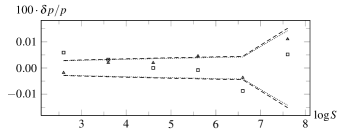
Figure 6: Relative difference of $\tilde{p}_{\mathrm{mc}}$ w.r.t. $\tilde{p}_{\mathrm{rw}}$ for $SW/(4a)=10^{-4}$, type (a) (dashed / squares), type (b) (dotted / triangles).

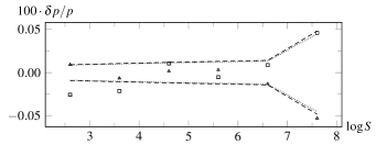
Figure 7: $SW/(4a)=10^{-3}$.

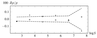
Figure 8: $SW/(4a)=10^{-2}$.

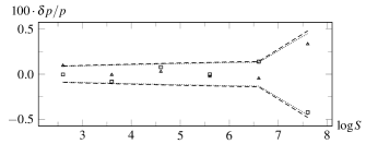
Figure 9: $SW/(4a)=10^{-1}$.

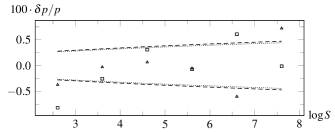
Figure 10: $SW/(4a)=10^{0}$.

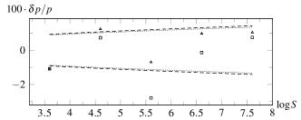
Figure 11: $SW/(4a)=10^{1}$.

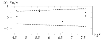
Figure 12: $SW/(4a)=10^{2}$.

Figures 13–16 show corresponding simulation results for rectangular lattices of varying aspect ratio. Here $S$ is constant for one plot. We restrict ourselves to $S=400$ and $S=4\times 10^{6}$ as examples of absolutely small and large lattices, respectively. Further, we keep the “regime” (in the original sense introduced for quadratic lattices) constant as well: for $S=400$, we choose $a/W=100$ and $a/W=10^{4}$, for $S=4\times 10^{6}$ we test with $a/W=10^{6}$ and $a/W=10^{8}$ (the latter figures belonging to the small-lattice regime), but note that the refined regimes for $L_{1}\neq L_{2}$ actually change when distorting the lattice. We have chosen our values so that the larger length $L_{1}$ exceeds the random walk length $\ell$ in the large-lattice regime throughout, and that it is much smaller than this length in the small-lattice regime for the quadratic case, but finally becoming much larger than it when distorting the lattice. Again, we show the relative error of simulations with respect to the random walk result in per cent, and plot a standard deviation (as obtained from $\tilde{p}_{\mathrm{rw}}$) corridor for comparison.

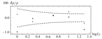
Figure 13: Relative difference of $\tilde{p}_{\mathrm{mc}}$ w.r.t. $\tilde{p}_{\mathrm{rw}}$ for $S=4\times 10^{2}$, $W/a=10^{-2}$, type (a) (dashed / squares), type (b) (dotted / triangles).

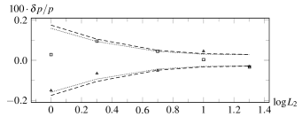
Figure 14: $S=4\times 10^{2}$, $W/a=10^{-4}$.

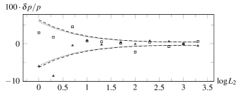
Figure 15: $S=4\times 10^{6}$, $W/a=10^{-6}$.

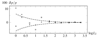
Figure 16: $S=4\times 10^{6}$, $W/a=10^{-8}$.

Appendix E Asymptotics of the truly one-dimensional result

For the one-dimensional symmetric random walk with structure function $\lambda(k)=\cos k$ and a lattice of $S\equiv L$ sites, we have

$$P^{*}(0;\xi)=\frac{1}{L}\sum_{m=0}^{L-1}\frac{1}{1-\xi\cos(2\pi m/L)}\,.$$ (59)

The identity of Appendix A in Montroll69 (with $w_{1}=\xi$, $w_{2}=0$, so that $\rho_{m_{1}}=\xi$ and $\phi_{m_{1}}\equiv 0$, and $x_{m_{1}}=[1-(1-\xi^{2})^{1/2}]/\xi$) then yields

$$P^{*}(0;\xi)=\frac{1}{\sqrt{1-\xi^{2}}}\frac{1+x_{m_{1}}^{L}}{1-x_{m_{1}}^{L}}=\frac{1}{\sqrt{1-\xi^{2}}}\frac{\xi^{L}+[1-(1-\xi^{2})^{1/2}]^{L}}{\xi^{L}-[1-(1-\xi^{2})^{1/2}]^{L}}\,.$$ (60)

For comparison with the asymptotic two-dimensional behavior, we evaluate the asymptotics of the 1d-expression for a ‘small’ lattice, i.e. for $L\ll\ell=\sqrt{\xi/(1-\xi)}$. Let $\alpha=\sqrt{1-\xi^{2}}\ll 1$, and note that this is not exactly the $\alpha$ of Montroll69 . However, $L/\ell\approx L\sqrt{1-\xi}=L\sqrt{1-\sqrt{1-\alpha^{2}}}\approx L\alpha/\sqrt{2}$, and since this is to be $\ll 1$, we can still use $L\alpha\ll 1$ in the following. With $1-\xi=1-\sqrt{1-\alpha^{2}}$ and $p_{\mathrm{rw}}^{-1}=L(1-\xi)P^{*}(0;\xi)$ we then obtain after minor manipulations

$$p_{\mathrm{rw,\,1d}}^{-1}=\frac{L[1-(1-\alpha^{2})^{1/2}]}{\alpha}\frac{1+\left(\frac{1-\alpha}{1+\alpha}\right)^{L/2}}{1-\left(\frac{1-\alpha}{1+\alpha}\right)^{L/2}}\,.$$ (61)

Straight-forward expansion in $L\alpha\ll 1$ yields

$$p_{\mathrm{rw,\,1d}}^{-1}=1+\frac{(L\alpha)^{2}}{12}+\mathcal{O}(L\alpha)^{3}\,,$$ (62)

where we omitted all terms of relative order $\alpha$. This is sufficient for the sought scaling limit $L\to\infty$, $\alpha\to 0$ while $L\alpha\simeq\mathrm{const.}$, and it is additionally justified by a Mathematica check of our calculations, which shows that the only interesting $\alpha$ orders left out in the result are terms of $\mathcal{O}(\alpha^{2})$ and thus much smaller than $(L\alpha)^{2}=L^{2}(1-\xi^{2})\approx 2(L/\ell)^{2}$.

Obviously, the most important difference compared to the 2d case is the absence of logarithmic terms, which are a characteristic sign of the marginal dimension two.

For completeness, let us also give the large-lattice asymptotics, i.e., for the case $L\alpha\gg 1$. Starting from the still exact (61), we use $(1-\alpha)/(1+\alpha)=1-2\alpha+\mathcal{O}(\alpha^{2})$. For $L\alpha\gg 1$, this raised to the $L/2$ power is much smaller than unity, the correct expansion thus reading $\exp(-L\alpha)(1+\mathcal{O}(L\alpha^{2}))$, and here we assume that terms of the latter relative order can be omitted as being much smaller than unity – this is an example that may be refined as necessary. One thus obtains the large-lattice result

$$\begin{split}p_{\mathrm{rw,\,1d}}&=\frac{2}{L\alpha}\left(1-2\operatorname{e}^{-L\alpha}+\mathcal{O}(\operatorname{e}^{-L\alpha}L\alpha^{2},\,\operatorname{e}^{-2L\alpha})\right)\\ &\approx\sqrt{2}\frac{\ell}{L}\left(1-2\operatorname{e}^{-\sqrt{2}L/\ell}\right)\,.\end{split}$$ (63)

Note that in this regime, the ratio of lengths no longer appears squared. In one dimension and for large lattices, the essential question for the encounter probability is whether the walker is deposited in the range $\ell$ from the target, and the probability for this to happen is the length ratio raised to the lattice dimension. The difference to the two-dimensional case is that the 1d random walk explores a dense region instead of a sponge-like structure.

Lastly, corresponding asymptotics for the extremely distorted version of the originally two-dimensional random walk are obtained by a mere rescaling $\ell\to\ell/\sqrt{2}$, as can be seen from Section 5.2.