Fluctuations of company yearly profits versus scaled revenue:
Fat tail distribution of Lévy type

Abstract

We analyze annual revenues and earnings data for the 500 largest-revenue U.S. companies during the period 1954-2007. We find that mean year profits are proportional to mean year revenues, exception made for few anomalous years, from which we postulate a linear relation between company expected mean profit and revenue. Mean annual revenues are used to scale both company profits and revenues. Annual profit fluctuations are obtained as difference between actual annual profit and its expected mean value, scaled by a power of the revenue to get a stationary behavior as a function of revenue. We find that profit fluctuations are broadly distributed having approximate power-law tails with a Lévy-type exponent $\alpha\simeq 1.7$, from which we derive the associated break-even probability distribution. The predictions are compared with empirical data.

Economics; econophysics, financial markets, business and management Time series analysis Fluctuation phenomena, random processes, noise, and Brownian motion

Predicting forthcoming year company profit is difficult due to the many unknown variables determining the actual earnings scenario. This intrinsic uncertainty in economy’s evolution makes earnings forecasts not to be correlated to actual earnings with the desired accuracy. A consequence is that, often, stocks with highest earnings forecasts dramatically underperfom those with poor forecasts (see e.g. [1]).

Indeed, company earnings may undergo dramatic variations from year-to-year, even over shorter time scales, leading to huge movements in public company stock (see e.g. [2]). A less volatile quantity is represented by total company revenue, but also in this case revenue variations may yield conspicuous changes in the underlying stock price. Interestingly, the connection between stock price (i.e. market value) and revenue is still surrounded by many open questions which are awating for further research (see e.g. [3]). Clearly, the question arises of how to estimate in a more realistic fashion profit fluctuations, and therefore attempting to improve the accuracy of earnings predictions, the latter being closely related to the issue of profitability or break-even point [4]. Several attempts have been made in order to incorporate a stochastic behavior of profits into the analysis (see e.g. [5, 6, 7, 8, 9, 10]), in which fluctuations are assumed to be normally distributed.

From a fundamental point of view, one may wonder whether the above difficulties can be mitigated to some extent by modifying the way the problem is approached. In physical many-body systems for example, a first, realistic solution to a problem can be achieved if one resorts to the so-called mean-field approximation, in which a single particle ‘sees’ an average field due to the remaining particles in the system (see e.g. [11, 12]). Particle-particle correlations and fluctuations of physical quantities can be incorporated into the formalism at a later stage once the mean-field solution of the problem is known (see e.g. [13]). How can we apply this idea to the study of profit fluctuations of real companies, which can be viewed as a many-particle system of interacting economic units? Is it possible to come up with the strong fluctuations observed in company profits?

Profit fluctuations can be naively evaluated by looking at their relative variations say, from year to year. As a matter of fact, however, profit is closely related to revenue and production costs (see below) and a different approach based on these interrelations could be explored.

In this Letter, we suggest that revenue can be taken as the independent, driving variable and present a novel analysis of profit fluctuations based on this assumption. We support our premises using market data from U.S. companies on an year-to-year basis over a period of 54 years. The analysis of the empirical data suggests a form for the expected mean profit, being a function of company revenue, with respect to which earnings fluctuations can be determined. The latter turn out to be dependent on revenue, suggesting that they are not stationary as a function of revenue. Invoking then the condition of stationarity, the fluctuations are scaled by a power of revenue with an exponent $\eta$ in the range $1/2<\eta<1$. The probability distribution function of scaled fluctuations displays slowly-decaying tails which turn out to be of Lévy type. A further analysis on the resulting break-even point yields a prediction, supported by empirical data, for the probability of profitability, enlightening the role that market fluctuations play in the problem.

In the following, we briefly review the standard cost-volume-profit (CVP) analysis, from which we derive our main conjectures regarding profit fluctuations. Let us consider a generic (typical) company. According to standard CVP analysis [14, 15], we write the profit $P$ as the difference between total revenue $R$ and costs, the latter being the sum of variable costs $V_{\rm c}$ and additional (sometimes referred to as fixed) costs $F\geq 0$, that is

$$P=R-(V_{\rm c}+F).$$ (1)

Further, we write total revenue as $R=v_{\rm s}n_{\rm s}$, where $v_{\rm s}$ is the sale price of sold unit and $n_{\rm s}$ the total number of sold units. Similarly, total variable costs are written as $V_{\rm c}=v_{\rm c}n_{\rm c}$, where $v_{\rm c}$ is the cost of produced unit and $n_{\rm c}$ is the total number of produced units.

In what follows, we assume linear relations between sold unit values and produced ones, according to

$$v_{\rm s} \simeq \alpha_{\rm s}~{}v_{\rm c},\qquad 1<\alpha_{\rm s},$$

$$n_{\rm s} \simeq \beta_{\rm s}~{}n_{\rm c},\qquad 0\leq\beta_{\rm s}\leq 1.$$ (2)

The above assumed linearities do not preclude the coefficients ($\alpha_{\rm s},\beta_{\rm s}$) to be time-dependent, similarly to a sort of piecewise linear approximation applied in non-linear CVP analysis [16]. Using these relations in Eq. (1), with $V_{\rm c}=R/(\alpha_{\rm s}\beta_{\rm s})$, yields

$$P=\gamma_{s}R-F,\quad{\rm with}\quad\gamma_{\rm s}={\alpha_{\rm s}\beta_{\rm s}-1\over\alpha_{\rm s}\beta_{\rm s}}.$$ (3)

Since we are interested in the typical behavior of companies, we write down the above $P$-$R$-$F$ relation in terms of its mean values, $P_{0}=\big{<}P\big{>}$, $R_{0}=\big{<}R\big{>}$ and $F_{0}=\big{<}F\big{>}$, representing averages of $P$, $R$ and $F$ over several companies for a given time horizon, say a year, i.e.

$$P_{0}=\big{<}\gamma_{\rm s}\big{>}R_{0}-F_{0}.$$ (4)

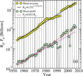
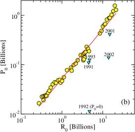
Figure 1: (color online) (a) Mean yearly revenue, $R_{0}$ [Billions] (circles) and mean yearly profit, $P_{0}$ [Billions] (squares) of the 500 largest revenue U.S. companies [17] as a function of the year. The thick straight line (top) is a fit with the form: $R_{0}=A_{0}\exp[({\rm year}-1954)/B_{0}]$ B, with $A_{0}=0.27$ and $B_{0}=12$. The dashed line (bottom) is the form: $P_{0}=A_{1}\exp[({\rm year}-1954)/B_{1}]$ B, with $A_{1}=0.014$ and $B_{1}=12$. The thin straight line is an exponential regression for $P_{0}$ over the whole years, yielding: $P_{0}^{\prime}=A_{2}\exp[({\rm year}-1954)/B_{2}]$ B, with $A_{2}=0.016$ and $B_{2}=13.8$, which is not proportional to $R_{0}$. (b) Mean yearly profit, $P_{0}$, vs mean yearly revenue, $R_{0}$ (circles) (from (a)). The straight line is the linear form $P_{0}=0.052R_{0}$. Anomalous-years results are indicated by the down triangles.

To test this relation, we consider the set of 500 largest revenue companies in the U.S. during the period (1954-2007) [17], for which yearly values of $P$ and $R$ are available. For each year in the database, we calculate the mean values $P_{0}$ and $R_{0}$ in billions (B) of U.S. dollars. Empirical results for $R_{0}$ and $P_{0}$ are plotted in Fig. 1(a) as a function of year. These results suggest that both quantities grow exponentially, and that $P_{0}\propto R_{0}$ if the anomalous years 1991/92/93 and 2001/02 are excluded. The exponential dependence of mean profit and revenue also reflects the growth of companies [18], displaying other interesting features described by exponential distribution functions.

Now, to better appreciate the apparent proportionality between mean profits and revenues, we have plotted them in Fig. 1(b), suggesting that indeed

$$P_{0}\simeq\big{<}\gamma_{\rm g}\big{>}R_{0},$$ (5)

with $\big{<}\gamma_{\rm g}\big{>}\cong 0.052$. Slight deviations from linearity can be observed in Fig. 1(b) at large revenues, $R_{0}>10$ B, corresponding to recent last years. This is an indication that, possibly, non-linear corrections to the result Eq. (5) are playing a role. In keeping with our mean-field strategy, however, we will consider such deviations as due to typical market fluctuations. Within this scenario, the model seems to be consistent with downward profit corrections for 2008, and possibly for the next few years, responding to a sort of reverse to the mean linear behavior obtained in Fig. 1(b). As a matter of fact, there is already a widespread consensus that 2008 is manifesting a rather weak economic environment. Furthermore, the linear relation between $P_{0}$ and $R_{0}$ then suggests that

$$F_{0}\simeq\big{<}\gamma_{\rm c}\big{>}R_{0},$$ (6)

such that

$$\big{<}\gamma_{\rm g}\big{>}=\big{<}\gamma_{\rm s}\big{>}-\big{<}\gamma_{\rm c}\big{>}.$$ (7)

Although we do not know $\big{<}\gamma_{\rm c}\big{>}$ explicitely, one can argue that $0<\big{<}\gamma_{\rm c}\big{>}<\big{<}\gamma_{\rm s}\big{>}$, as one would expect from the definition of $F$ (see Eq. (1)) and the fact that $\big{<}\gamma_{\rm g}\big{>}>0$. Now, writing $\big{<}\gamma_{\rm s}\big{>}=1-\big{<}1/(\alpha_{\rm s}\beta_{\rm s})\big{>}$, we can estimate the last term by assuming $\big{<}1/(\alpha_{\rm s}\beta_{\rm s})\big{>}\simeq 1/\big{<}\alpha_{\rm s}\beta_{\rm s}\big{>}$. Accordingly, we find that on average

$$\big{<}\alpha_{\rm s}\beta_{\rm s}\big{>}\simeq\frac{1}{1-(\big{<}\gamma_{\rm g}\big{>}+\big{<}\gamma_{\rm c}\big{>})},$$ (8)

hence $\big{<}\alpha_{\rm s}\beta_{\rm s}\big{>}>1/(1-\big{<}\gamma_{\rm g}\big{>})\simeq 1.062$ and $\big{<}\gamma_{\rm s}\big{>}>0.058$, implying that $\big{<}\gamma_{\rm c}\big{>}>0.006$.

The linear relation between $P_{0}$ and $R_{0}$ is obtained when the anomalous years (1991, 1992, 1993, 2001 and 2002, see Fig. 1(a)) are excluded from the exponential fit. If these anomalous years are included in the fit, an exponential regression for $P_{0}$ (see the thin straight line in Fig. 1(a)) yields a non-linear relation between $P_{0}$ and $R_{0}$. In the light of these results we may argue that companies show typical profit-revenue scenario when both variables are linearly related to each other, at least in an average sense. Departures from linearity, as the down-triangles shown in Fig. 1(b), may be referred to as extremal, non-typical events. Indeed, the cause for such strong deviations from the linear relation between $P_{0}$ and $R_{0}$ can be traced back to specific historical facts.

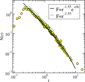
Figure 2: (color online) Distribution function of revenues $N(r)$ vs scaled revenue $r=R/R_{0}$ (circles). The continuous line is a fit with the form: $n(r)=0.3~{}r^{-1.55}\exp(-r/6)$ for $r>0.2$. The straight line is the power-law form: $n(r)\sim r^{-1.55}$ (valid within the interval $0.3\lesssim r\lesssim 2$).

The simple exponential fit for $R_{0}$ shown in Fig. 1(a) will be used in the following to scale annual revenues and profits, to take into account the year-to-year variations due to the exponential growth in economic activity. One example of such scaled quantities is the revenue itself for which we have calculated the probability distribution function (PDF) $N(r)$ of scaled revenues $r=R/R_{0}$. The results are shown in Fig. 2. The scaled revenue PDF $N(r)$ displays an intermediate power-law regime with decaying exponent $\simeq-1.55$ followed by an exponential tail for large $r$. In what follows, scaled profits will be denoted as $p=P/R_{0}$.

Next, we study the issue of profit fluctuations by considering again a generic company having scaled profit $p$ and revenue $r$, at any given year within our database. Profit fluctuations will be considered to be a function of scaled revenue $r$, rather than a function of time. Profit fluctuation, denoted as $\Delta p$, is defined as the difference between actual $p$ and its expected mean value, here denoted as $\bar{p}$, i. e.

$$\Delta p=p-\bar{p}.$$ (9)

In order to determine the expected mean profit $\bar{p}$, we have plotted all available values of $p$ and $r$ in our database (including the anomalous years) and performed a linear regression to the data which should represent the behavior of $\bar{p}$ vs $r$. The fit, $\bar{p}\simeq a+br$ (not shown here), yields a rather small intercept value, $a\simeq-0.004$, which can be neglected for our present purposes, while $b\simeq 0.056$. Therefore, we postulate that the expected mean profit $\bar{p}$ is a function of $r$ and obeying

$$\bar{p}=\big{<}\gamma_{\rm g}\big{>}r,\quad{\rm with}\quad\big{<}\gamma_{\rm g}\big{>}\cong 0.052.$$ (10)

We will explain below the reason for choosing the above value for $\big{<}\gamma_{\rm g}\big{>}$. Thus, in the present context, company mean profit is a function of solely actual company revenue $r$, times a global market parameter $\big{<}\gamma_{\rm g}\big{>}$, which is taken the same for all companies. Later, we will relax the latter condition and discuss the consequences of taken instead a different proportionality factor $\gamma_{\rm g}$ for each individual company. Note that by averaging Eq. (10) over all companies and years we get $\big{<}\bar{p}\big{>}\equiv P_{0}/R_{0}=\big{<}\gamma_{\rm g}\big{>}$, consistent with the empirical result Eq. (5). We have also checked that $r\sim 1$ and fluctuations of $r$ are essentially stationary all over the period considered.

The fluctuations Eq. (9) can be scaled by using a characteristic value, such as the standard deviation, $\sigma_{\rm p}$, provided that the second moment of the distribution be finite. Alternatively, one can use a lower-order moment such as $\big{<}|\Delta p|\big{>}$ to characterize the amplitude of profit fluctuations.

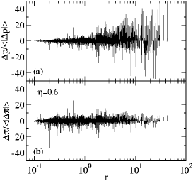
Figure 3: (color online) (a) Scaled profit fluctuations $\Delta p/\big{<}|\Delta p|\big{>}$ vs scaled revenue $r=R/R_{0}$, with $\big{<}|\Delta p|\big{>}=0.034$. (b) Renormalized scaled profit fluctuations $\Delta\pi/\big{<}|\Delta\pi|\big{>}$ vs $r$, where $\Delta\pi=\Delta p/r^{\eta}$, with $\eta=0.6$ and $\big{<}|\Delta\pi|\big{>}\simeq 0.030$.

Values of $\Delta p$ are plotted in Fig. 3(a) versus scaled revenue $r$. As one can see from the plot, profit fluctuations are not ‘stationary’ as a function of $r$, their amplitudes tend to grow with $r$; the larger the revenue the larger the amplitude of profit fluctuations. In the following, we wish to quantify the observed rate of growth of amplitude fluctuations with revenue and, as a result, being able to find out a source of profit fluctuations which is stationary as a function of $r$. To achieve this, we suggest that a suitable variable describing fluctuations is given by

$$\Delta\pi=\frac{\Delta p}{r^{\eta}},$$ (11)

with $\eta\geq 0$. The question arises of how to determine $\eta$. To do this, we look at the mean-square fluctuations of the data, $\sigma^{2}_{\eta}=\big{<}(\Delta\pi(\eta))^{2}\big{>}-\big{<}\Delta\pi(\eta)\big{>}^{2}$, for fixed $\eta$, and search for the minimum of $\sigma^{2}_{\eta}$ as a function of $\eta$. We find a minimum value $\sigma_{\eta}\simeq 0.051$ for $\eta\simeq 0.6$. The resulting scaled fluctuations $\Delta\pi/\big{<}|\Delta\pi|\big{>}$ are reported in Fig. 3(b) versus $r$, displaying a satisfactory stationarity. The value of $\eta$ thus obtained does not guarantee the vanishing of the first moment $\big{<}\Delta\pi\big{>}$. A fine tuning of the value of $\big{<}\gamma_{\rm g}\big{>}$, which enters Eq. (9) and Eq. (10), can be accurately performed in order that $\big{<}\Delta\pi\big{>}=0$. This is achieved for $\big{<}\gamma_{\rm g}\big{>}\simeq 0.052$, the value used in the discussions above.

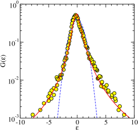
Figure 4: (color online) PDF of scaled profit fluctuations $G(\epsilon)$ versus $\epsilon=\Delta\pi/\big{<}|\Delta\pi|\big{>}$, for $\eta=0.6$ (circles). The continuous line is a fit with the form: $F=a/(1+|\epsilon/b|+|\epsilon/c|^{2.7})$, with $a=0.55$, $b=0.6$ and $c=0.9$ for $\epsilon\leq 0$, and $F=a/(1+|\epsilon/c|^{2.7})$ with $a=0.55$ and $c=0.75$, for $\epsilon\geq 0$, implying power-law tails with a Lévy-like exponent $\alpha=1.7$. The dashed line is the normal distribution.

It is remarkable that $\eta\neq 0.5$, the latter would indicate a standard behavior of fluctuations. The fact that $\eta>1/2$ tells us that fluctuations are stronger than one would expect if $\Delta\pi$ were normally distributed (see e.g. [6]). To find out the actual shape of the probability distribution function, $G(\epsilon)$, for $\epsilon\equiv\Delta\pi/\big{<}|\Delta\pi|\big{>}$ (in the case $\eta=0.6$), we have plotted it in Fig. 4. As one can see, the shape of $G(\epsilon)$ is consistent with a power-law decay at the tails with a Lévy-like exponent $\alpha=1.7$. The negative tail of $G(\epsilon)$ somehow reflects the fact that companies with poor revenue behavior can be taken out of the Fortune 500 set and it may thus become underweighted. Similar arguments are used in discussing fund performance (see e.g. [19, 20]) but a thorough understanding of this phenomenon calls for further studies. To be noted is that processes resulting from other human-based activity, such as price variations in financial markets (see e.g. [21]), speed fluctuations of an ensemble of cars in a closed circuit traffic [22], just to name a few examples, also display strongly fluctuating features typically characterized by fat-tail distributions.

We can make contact with the above obtained value of $\eta$ by arguing that indeed $\eta=1/\alpha$. To see this, let us write the relation $\epsilon\equiv\Delta\pi/\big{<}|\Delta\pi|\big{>}$ as follows

$$p=\big{<}\gamma_{\rm g}\big{>}r+\big{<}|\Delta\pi|\big{>}r^{\eta}\epsilon,$$ (12)

suggesting that profit $p$ is driven ‘deterministically’ by the first term proportional to revenue $r$, plus a second fluctuating term where amplitude fluctuations are also determined by revenue, but to some power $\eta$. From a physical point of view, the first term represents a driving or bias field and the second one a stochastic part due to an external random force acting on the system (see e.g. [23]). Such a model resembles very closely the simple approach due to Bachelier [24] for describing the temporal evolution of stock prices. In our approach, time is replaced by revenue and $\epsilon$ is not normally distributed (see also [25]).

Now, imagine we can write the factor $r^{\eta}\epsilon$ as a sum over independent, identically distributed (according to $G(\epsilon)$) Lévy-like variables $\epsilon_{i}$, such that

$$r^{\eta}\epsilon=a\sum_{i=1}^{n_{r}}\epsilon_{i},$$ (13)

where $a>0$ is a constant and $n_{r}$ depends on $r$. A similar picture has been used for the description of seed production of forests [26]. Invoking the stability of Lévy distributions, the above sum is also Lévy distributed with the same exponent $\alpha$ as the single variable, obeying the scaling relation, $\sum_{i=1}^{n_{r}}\epsilon_{i}\simeq\epsilon^{\prime}n_{r}^{1/\alpha}$ (see e.g. [27]). Even if the random variables $\epsilon$ are not independent, but long-range autocorrelated, the sum scales as $n_{r}^{H}$, where the Hurst exponent $H$ is expected to be $H\simeq 1/\alpha$ (see e.g. [28]). Details of the corresponding correlations analysis will be discussed elsewhere.

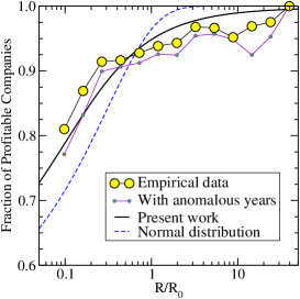
Figure 5: (color online) Fraction of profitable (Fortune 500) companies in the U.S. in the period (1954-2007) (circles) versus scaled revenue $r=R/R_{0}$. The continuous line is the prediction from the present work. The dashed line the one from a normal distribution of profit fluctuations.

Assuming now that the number $n_{r}$ is proportional to revenue in the form $n_{r}=r/r_{b}$, with $r_{b}$ arbitrarily small, we find according to Eq. (13), that

$$r^{\eta}\epsilon=a\epsilon^{\prime}\frac{r^{1/\alpha}}{r_{b}^{1/\alpha}}.$$ (14)

Identifying the parameter $a$ in the form $a=r_{b}^{1/\alpha}$ and noting that $\epsilon^{\prime}\sim\epsilon$, we arrive at the relation $\eta=1/\alpha$ claimed above. The values of $\eta$ and $\alpha$ obtained here are consistent with this prediction.

In what follows, we will elaborate our findings further to consider the issue of profitability, admittedly important for being able to make predictions about the probability for a generic company to be profitable. This is related to the concept of break-even or point at which profits vanish. The idea here is to estimate the probability of profitability as a function of revenue $r$ by appropriately taking into account profit fluctuations due to statistical market variations.

Our derivation starts from Eq. (12), with $\eta$ substituted by $1/\alpha$, i.e. $p=\big{<}\gamma_{\rm g}\big{>}r+\big{<}|\Delta\pi|\big{>}r^{1/\alpha}\epsilon$, with $\alpha\simeq 1.7$. At break-even (BE), $p=0$ and the above relation suggests that, $\epsilon=-\big{<}\gamma_{\rm g}\big{>}r^{1-1/\alpha}/\big{<}|\Delta\pi|\big{>}\equiv-\epsilon_{\rm BE}$, where

$$\epsilon_{\rm BE}=\frac{\big{<}\gamma_{\rm g}\big{>}}{\big{<}|\Delta\pi|\big{>}}r^{1-1/\alpha},$$ (15)

which is positive since here $\big{<}\gamma_{\rm g}\big{>}>0$. Now, we define the probability for a generic company to be profitable, $P_{\rm PF}(r)$, as the fraction of all events for which the fluctuating variable $\epsilon\geq-\epsilon_{\rm BE}$, since in these cases profit becomes positive, $p>0$. The probability of profitability can be conveniently expressed as the integral (see also [9])

$$P_{\rm PF}(r)=\int_{-\epsilon_{\rm BE}}^{\infty}d\epsilon~{}G(\epsilon),$$ (16)

which is a function of $r$ through $\epsilon_{\rm BE}$. One may argue that values $\epsilon\to\infty$ are not realistic, requiring the introduction of an effective upper cut-off for $\epsilon$, that we can denote as $\epsilon_{\rm cut}$. We find that the results become indistinguishable from those obtained from Eq. (16) when $\epsilon_{\rm cut}>8-10$, consistent with the range of variations of $\epsilon$ obtained in Fig. 4. Thus, for simplicity, we take the upper integration limit in Eq. (16) as $\epsilon\to\infty$.

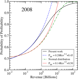
Figure 6: (color online) Probability of profitability $P_{\rm PF}$ versus revenue [Billions] predicted for 2008 for a typical company. The continuous line is the theoretical prediction Eq. (16) and the dashed line the linear approximation valid for small revenues (here $R\lesssim 0.5$ B). The dot-dashed line is the prediction from the normal distribution and the thin line the corresponding asymptotic linear form.

Numerical results are shown in Fig. 5, where a comparison is made with the total fraction of profitable companies in the period 1954-2007 with respect to the total number of companies as a function of scaled revenue. The large circles refer to ‘typical’ years, excluding the anomalous ones. If the latter are also included, the fraction of profitability decreases a bit. Our theoretical prediction works satisfactorily well, justifying a posteriori the few ad-hoc assumptions made in this work. The dashed line is the theoretical prediction in the case in which $\eta=1/2$ and $G(\epsilon)$ be the normal distribution, clearly yielding a poorer description of the empirical results.

Based on these results, we can make predictions for 2008 using the expected mean revenue $R_{0}\simeq 24.3$ B. The results of profitability as a function of absolute revenue $R$ (in billions) are displayed in Fig. 6. Linear approximations, valid for small revenues, are also reported in the plot to help making simple estimates for small revenue companies.

Our results are based on the use of the mean (and positive) growth factor $\big{<}\gamma_{\rm g}\big{>}$ determining expected profits. This was done as an attempt to describe a generic, typical company. Now, actual companies may behave quite differently than this typical behavior. This can be taken into account by considering, instead of $\big{<}\gamma_{\rm g}\big{>}$, the actual company-dependent driving factor $\gamma_{\rm g}=\gamma_{\rm s}-\gamma_{\rm c}$, that is the counterpart of Eq. (7), such that

$$\bar{p}=\gamma_{\rm g}r=(\gamma_{\rm s}-\gamma_{\rm c})r.$$ (17)

Here, the factor $\gamma_{\rm c}$ relates (fixed) costs $F$ to revenue as $F=\gamma_{\rm c}R$, which in the scaled form becomes $f=F/R_{0}=\gamma_{\rm c}r$.

The present break-even and profitability results, valid for a typical company, can still be applied to a single company with the condition that the break-even value is calculated according to the particular value of $\gamma_{\rm g}$. The result is

$$\epsilon_{\rm BE}=\frac{(\gamma_{\rm s}-\gamma_{\rm c})}{\big{<}|\Delta\pi|\big{>}}r^{1-1/\alpha},$$ (18)

which can become negative if $\gamma_{\rm s}<\gamma_{\rm c}$. In the case $\gamma_{\rm g}>0$, also $\epsilon_{\rm BE}>0$, and the previous conclusions for $P_{\rm PF}(r)$ still apply. When $\gamma_{\rm g}<0$, then $\epsilon_{\rm BE}<0$ and the lower integration limit in Eq. (16) becomes positive, yielding lower values of $P_{\rm PF}(r)$ as compared to $P_{\rm PF}(r)$ with the same revenue $r$ but positive $\gamma_{\rm g}$. Thus, for a single company the problem reduces to estimate accurately the growth factors $\gamma_{\rm s}$ and $\gamma_{\rm c}$ in each particular scenario.

In summary, we have analyzed annual profits and revenues of U.S. companies over a period of 54 years. We find a linear relation between annual mean profit ($P_{0}$) and revenue ($R_{0}$), which is at the basis of the concept of typical company or mean-profit-revenue relation. In the ‘typical economy’ picture discussed here, expected mean profits behave directly proportional to revenue, the latter being the driving variable. Furthermore, conjectures allow us to study profit fluctuations depending on actual revenue plus a fluctuating term governed by a distribution function of a Lévy type. Strong deviations from the expected typical behavior of companies can be referred to as extremal, non-typical events. Indeed, within the 54 years data considered few extreme events (years) are observed for which profits and revenues display strong deviations from the linear relation between $P_{0}$ and $R_{0}$. However, such deviations can be traced back to specific historical facts and the corresponding years may be considered as non-typical ones.

Although our conclusions are based on the study of the highest revenue companies in the U.S., we believe that our results still possess a robust degree of universality to be of more general validity, and can be used as a benchmark from which one can predict forthcoming profit-revenue scenarios. As an application, the present analysis has been used to estimate the probability that a single company has in order to become profitable. The analyzed empirical data are in support of our suggestions.

- [1] M. Hwang Smith, M. Keil and G. Smith, Applied Financial Economics 14, 937-943 (2004)
- [2] R. Jennings and L. Starks, The Journal of Finance XLI, 107 (1986)
- [3] V.J. Cook, Jr., The Value/Revenue Ratio: A Semi-Long-Wave Marketing/Accounting Metric (working paper, Tulane University, 2007 (SSRN Nr. 961167))
- [4] R.W. Hilton, Managerial Accounting: Creating Value in a Dynamic Business Environment, Sixth Edition (McGraw-Hill, Irwin, 2005)
- [5] R.K. Jaedicke and A.A. Robichek, Accounting Review 39, 917-926 (1964)
- [6] C. Kim, Decision Sciences 4, 329 (1973)
- [7] Z. Adar, A. Barnea and B. Lev, The Accounting Review 52, 137-149 (1977)
- [8] J.F. Kottas and H.-S. Lau, The Accounting Review 53, 247-251 (1978)
- [9] J.A. Yunker and P.J. Yunker, J. of Accounting Education 21, 339-365 (2003)
- [10] J.A. Yunker and D. Schofield, Managerial and Decision Economics 26, 191-201 (2005)
- [11] G. Parisi, Statistical field theory (Perseus Books Publishing, U.S., 1988)
- [12] P.M. Chaikin and T.C. Lubensky, Principles of condensed matter physics (Cambridge University Press, Cambridge, 1995)
- [13] R.A. Broglia, G. Coló, G. Onida and H.E. Roman, Solid state physics of finite systems: Metal clusters, fullerenes, atomic wires (Advanced Texts in Physics, Springer Verlag, Berlin 2004)
- [14] D. Colander, Economics (MacGraw-Hill, New York, 2004)
- [15] J. Soper, Mathematics for Economics and Business (Blackwell Publishing, Oxford, 2004)
- [16] W.-H. Tsai and T.-M. Lin, Engineering Costs and Production Economics 20, 81 (1990)
- [17] Fortune 500, http://money.cnn.com/magazines/fortune.
- [18] M.H.R. Stanley, L.A.N. Amaral, S.V. Buldyrev, S. Havlin, H. Leschhorn, P. Maass, M.A. Salinger and H.E. Stanley, Nature 379, 804 (1996)
- [19] S.J. Brown, W. Goetzmann, R.G. Ibbotson and S.A. Ross, The Review of Financial Studies 5, 553 (1992)
- [20] E.J. Elton, M.J. Gruber and C.R. Blake, The Review of Financial Studies 9, 1097 (1996)
- [21] R.N. Mantegna and H.E. Stanley, Nature 376, 46 (1995)
- [22] H.E. Roman, F. Croccolo, C. Riccardi, Physica A 387, 5575 (2008)
- [23] N.G. van Kampen, Stochastic processes in physics and chemistry (Noth-Holland, Amsterdam, 1981)
- [24] L. Bachelier, Theorie de la Speculation, Annales Scientifiques de l’Ecole Normale Supérieure III-17, 21 (1900)
- [25] J.C. Hull, Options, Futures and Other Derivatives (Prentice-Hall, Upper Saddle River NJ, 1997).
- [26] Z. Eisler, I. Bartos and J. Kertész, Advances in Physics 57, 89 (2008)
- [27] R.N. Mantegna and H.E. Stanley, An Introduction to Econophysics (Cambridge University Press, Cambridge, 2000)
- [28] G. Samorodnitsky and M.S. Taqqu, Stable Non-Gaussian Random Processes: Stochastic Models with Infinite Variance (Chapman and Hall/CRC, Boca Raton, 1994)