A self-confined Fermi-gas model for nuclear collective motion
V.P. Aleshin
Institute for Nuclear Research, Kiev, 03680, Ukraine
Abstract
The well-known phenomenological dynamic equation for the nuclear shape parameter was derived from first principles with the aim of obtaining the microscopic or many-body expressions for inertia , deformation force , and friction coefficient of collective motion in hot nuclei. Nuclear evolution, viewed as a sequence of quasiequilibrium stages, is described with the aid of the density matrix constrained to given expectation values of nuclear Hamiltonian , number operator , and operators , , and of coordinate, momentum, and inertia of collective motion. Having chosen an explicit expression for in terms of the nucleon field operators , , we construct the corresponding expressions for , , and , using a certain canonical transformation of , , the equation of continuity and an assumption that the collective variables where are Heisenberg representations of , , , change with time much slower than the number density and the momentum density, from which are built. The same assumption was used to get the closed-form solutions of the dynamic equations for , from which we extract the desired many-body expressions for , , and . After adaptation of those general expressions to a self-confined Fermi gas with the phenomenological effective force, they are used for critical analysis of the previous microscopic models of those quantities and for elucidating the distinctive features of dissipative collective motion in atomic nuclei.
PACS numbers: 25.70.Lm, 24.10.Cn, 25.70.Jj
1 Introduction
Collective or ’macroscopic’ motion of atomic nuclei consists in large-scale deformations of nuclear shape, characterized by the parameter , which satisfies the equation of motion
| (1) |
with , , in which inertia , deformation force , and friction are certain functions of . Suggested in [1, 2, 3] for neutron-induced fission, Eq. (1), after coupling to particle evaporation from strongly deformed nuclei [4] and completing by a random force [5, 6], has become a promising tool for an in-depth analysis of experimental data on fusion-fission, fusion-evaporation and quasifission processes following nucleus-nucleus collisions at the energies per nucleon sizably below the Fermi-energy [7, 8, 9, 10].
The microscopic content of , , , and is obscure, because Eq. (1) has never been derived, as a whole, from quantum-statistical theory of self-bound nonequilibrium Fermi systems. This work suggests such a derivation, under hypothesis that Eq. (1) is a consequence of the dynamic equations for ’macroscopic’, ’gross’ or collective variables of the system.
The first step towards microscopic interpretation of (1) was made in [11, 12] by postulating the microscopic expressions for and . The first of those is very simple
| (2) |
where is the number density, while is some function of , whose integral with the spherically symmetric distribution equals 0. The was taken in the form , where is a certain functional of only [12]. Four parameters of this functional: central density, compression modulus, central energy density, and a quantity controlling the diffuseness of the nuclear surface, were treated phenomenologically. The expressions for and were used in the variational problem
| (3) |
whose solution provides the number density for the nucleus with the particle number and deformation . Although Eq. (3) closely resembles the equation for electronic density in the ground state of a diatom molecule at frozen internuclear distance, with being the analog of the sum of the electronic kinetic energy in Thomas-Fermi approximation and the interelectronic interaction, and being the similitude of the electron-nuclei potential, the authors [12] insist that and in (3) are the total energy and number density averaged over a group of levels of a nucleus with fixed and over .
The in the expression is known as the deformation potential. From the above we see that in Ref. [12] it is identified in fact with the internal (or thermal) energy . This contradicts to many other works (see [6], and references therein), interpreting as Helmholtz’s free energy either without proof or by assuming that the process of deformation of a hot nucleus is similar to compression or decompression of a gas embedded in a heat bath with a fixed temperature and occurring so slowly that the temperature of the gas always coincides with that of the heat bath. Evidently this analogy is misleading, because the temperature of the nucleus in the process of deformation is increasing.
For cold nuclei the is identified with the ground state energy of a nucleus with fixed and . This allows one to obtain it by minimizing the expectation of the total Hamiltonian with a state subject to the condition . Here, is the operator of collective coordinate
| (4) |
where is the number density operator and is the same as in (2). To simplify this variational problem, the is replaced by a single Slater determinant of single-’particle’ wave functions and, to compensate for such a severe restriction of the Hilbert space, the bare internucleon interaction in the expression for is replaced by the effective force. This leads to the so-called self-consistent mean-field (SCMF) models. In the early stage [13], most SCMF calculations have used effective forces of the Skyrme type [14] revived by Vautherin and Brink [15, 16]. Nowadays [17], the three most widely used variants of SCMF’s are based on a Skyrme energy functional, a Gogny force [18], and a relativistic mean-field Lagrangian [19].
To justify description of many-particle systems with strong interparticle interactions with the aid of the SCMF model it is necessary to assume [20] that only the two-particle scatterings, influenced by the media, are essential, while the three- and more particle collisions are negligible. Moreover, the coalescence of few nucleons into a cluster is prohibited. It is hardly possible to validate those assumptions for real nuclei. Therefore we trust in the SCMF models simply because with several parameters in the effective force, adjusted for a few reference nuclei, they reproduce very good the binding energies and densities of many other nuclei [17].
Encouraged by good performance of the SCMF theory in studies of these quantities, Flocard et al [21] apply it with a reasonable success to explore the two-humped fission barrier in 240Pu addressed before within the shell-correction approach [22]. Excellent reproduction of fission barriers for 240Pu and other acitinide nuclei, obtained later with the Skyrme force named SkM∗ [23], seems mysterious, because the identification of the fission path with a sequence of ground states at fixed is in apparent conflict with the compound nucleus model of fission, used to deduce the fission barriers from experimental excitation functions.
It is well known that for the inertial parameter in Eq. (1) the hydrodynamic formula [3] is used by far more often than any other. This poses the problem of the microscopic interpretation of this formula, to the solution of which most close is the adiabatic time-dependent Hartree-Fock (ATDHF) theory [24, 25, 26]. A nonstationary state vector of the nucleus is generated in this theory by appending to the Slater determinant a phase factor , where is a small, time-even, nonlocal one-body operator. Assuming that has the form , with , one expands the energy in powers of , stops at second order, and dropping the term from time reversal symmetry, one gets
where
has the form of the inertia parameter of an abstract fluid with a mass density and a velocity potential . It should be stressed, however, that the expression is only a rough estimate of the solution of very involved equations for . Moreover, the velocity potential is not proved to satisfy the Laplace equation and it is chosen heuristically.
Turning to microscopic expressions for friction , we remark that for quite a long time [27, 28, 29, 30, 31, 32, 33, 34] they were extracted from the linear response function of a thermally equilibrated Fermi gas confined by the external forces on the small variations of those forces. And only recently [35] it has been realized that in the bulk of such a gas, there will be no mass flow, , defined as the expectation of the momentum density operator
| (5) |
with the density matrix of the system. Therefore, the collective motion, hence the dissipation of collective energy in such a gas will be confined to the area of the nuclear surface. Having recognized this fact we have constructed the Rayleigh dissipation function from the entropy production rate for the canonical ensemble subject to the constraint , where over the entire nucleus. Although the final expressions for in [35] look reasonable, their derivation is far from convincing. First, the was not constrained from the beginning by the condition , instead of which the deformation was introduced in only in the final stage of derivation in an intuitive way. Second, having postulated for the mass flow the hydrodynamic-like formula: , we failed to reveal the microscopic content of the ’fluid velocity’ , which was treated instead according to the model of Hill and Wheeler [3].
The main objective of this paper is the derivation of Eq. (1) from first principles and removing in this way all the obscurities in microscopic interpretations of , , and , mentioned above. Skipping for simplicity the spin and isospin indices and letting , as done already in (5), the total energy and number operators are written as
| (6) |
| (7) |
in terms of the field operators , , which satisfy the anticommutation relations
| (8) |
and a ’bare’ NN-interaction . In order to furnish the formal description of macroscopic motion in a nucleus with total particle number and total energy , Eqs. (6), (7) for and must be supplemented by explicit expressions in terms of , for the set of coordinate, momentum, and inertia of this motion. Denoting as the expectation values of with yet unknown time-dependent density matrix, we postulate that those are very slow functions of . In formal terms this signifies that the time axis can be broken up into succession of intervals , where is small enough for the expressions
| (9) |
to hold for all , but yet sufficiently large compared to the internal characteristic times to justify description of the nucleus within the corresponding interval of by the density matrix , which maximizes the entropy under the following constraints
| (10) |
According to this definition suggested by Jaynes [36], the does not depend on the local time of the stage in question. The dependence is attached to the observables: , where are functionals of , . In particular the values of at the beginning of the next to stage are given by , which solves, in principle at least, the whole problem of collective or macroscopic motion.
The operator is given in (4). The operators and are expected to be linear functionals of the momentum density and number density , respectively, subject to the conditions
with [24]. But those conditions alone do not determine the weighting functions in and in a unique way. Moreover, the equation shows that, given , there are correlations between and , whereas the constraining conditions in Jaynes’s definition of are mutually independent. As shown in section 2, all these difficulties in constructing are avoided by imposing on the following restriction
where the is the canonical density matrix, which satisfies the conditions , and depends on yet unspecified inverted temperature , whereas is yet unknown real function of the nucleon position . In order to work out the equations for and , we use the continuity equation and assume that macroscopic variables change with time much slower than the number and momentum densities, and , through which those are defined, the argument being that after spatial integrations, invoked in those definitions only the slow components , of , survive. Having postulated explicit expressions for , , we complete the definition of and , the net result being that the is now completely defined, which allows one to use Eq. (10) for the definition of the weighting functions in and in a unique way.
In section 3 we utilize another, besides (9), an implication of the adiabaticity hypothesis to get the closed-form solution of the dynamic equation for the expectation of , , and use this solution to express the quotient as a function of the quotient and . After replacement of those quotients with the derivatives, this expression takes the form of equation (1) for , which permits us to get the many-body expressions for , , and .
In section 4, we use the results of Refs. [37, 38, 39, 40] to construct the self-confined Fermi gas (SCFG) model, which is a natural extension of the self-consistent mean field model of ground state nuclei with fixed shape, to hot nuclei. The expressions for , , and obtained for the self-confined Fermi gas from our general theory of nuclear collective motion are compared with the previous models of those quantities. In section 5 we give a short summary of our main conclusions and elucidate the physical nature of collective motion in hot nuclei.
2 The quasiequilibrium density matrix
2.1 General expressions for
In this section we define the quasiequilibrium density matrix of the system on a separate stage of collective motion, which lasts between and . This does not depend on the local time , while all observables depend on according to the low
| (11) |
where . The values of and are denoted as and , respectively. The total number and the total energy of the system are and .
Given , the canonical density matrix of the nucleus reads
| (12) |
| (13) |
where the and are functions of , , , determined from the equations
| (14) |
with respect to , , while the inverted temperature will be specified later. Putting into (14) the definitions (7), (4) of and , respectively, and introducing the number density
| (15) |
we rewrite the equations for and in the form
| (16) |
from which it follows that
| (17) |
| (18) |
The mass flow in equals 0:
| (19) |
because , being a function of even operator , is itself even under a time-reversal transformation, while is odd. In order to find the general form of with , we use the analogy with the classical fluid with the velocity . According to Mori [41] the distribution function of such a fluid, consisting of particles of mass with coordinates and momenta, is obtained from that of the fluid with by the substitutions
| (20) |
Keeping in mind that (20) is the canonical transformation, because , obey the same Poisson bracket as , , and that in quantum systems of identical particles the role of and is taken over by , , we therefore define the density matrix with as follows
where , must satisfy the canonical anticommutation relations (8) and give rise to the primed densities
| (21) |
obeying the conditions
| (22) |
with being the nucleon mass and an yet unknown c-number vector function. Eqs. (22) have exactly the same form as the relationships, following from Eqs. (20), between the corresponding densities in the classical fluid.
It is readily seen that the required , have the form
| (23) |
where is a real function remaining to be determined. Really, the fulfillment of anticommutation relations and of the first condition in (22) is evident, while substitution of (23) into defined in (21) leads to the second condition in (22) with
| (24) |
The trace of any functional of the nucleon field operators is
| (25) |
being the state with no particles. By definition, the primed trace is obtained from by putting primes on those and , which explicitly appear in (25), but not on those hidden in . From (23) then follows the formula , which leads at with accounting for to the useful relationship
| (26) |
As a first application of (26) consider the mass flow in :
| (27) |
From (26) and the expression
| (28) |
which follows from (22), one obtains
| (29) |
By definition, the primed counterpart of any operator , including the trace, is expressed in terms of , in the same way that the corresponding unprimed operator is expressed in terms of , . Since, in addition, , obey the same anticommutator relations as , , one can drop all primes in (29). Then, using (19), (15) yields
| (30) |
Let us now employ Eq. (26) at to calculate the entropy in the ensemble. Use of leads to , or on removal of all primes,
where is the entropy of the ensemble.
In passing we note that and given in (23) can be put into the form
| (31) |
where
| (32) |
will be called the phase operator. This is proven by application of the formula
| (33) |
at and , and the expressions
Eq. (31) allows the definition of any primed operator to be written as
| (34) |
For on remarking that , Eq. (34) becomes
| (35) |
This formula for is analogous to the definition of the density matrix of the time dependent Hartree-Fock formalism [25, 26], in which, however, the operator analogous to our , Eq. (32), is nonlocal, while that analogous to represents a time-even Slater determinant.
2.2 The definitions of and
With Eq. (12) for , the definition implies that
| (36) |
where , , and are constructed from and in the same way that , , and are constructed from and . Use of Eqs. (6), (7), (4) for , , , respectively, and Eq. (24) for leads to the expressions
| (37) |
, , so that (36) becomes
| (38) |
where . In this subsection we formulate the equations for still unknown parameters and of by exploiting the adiabaticity of collective motion and the continuity equation.
To embody the slowness of collective variables in their formal definition introduce the number density at time
| (39) |
For , reduces to
| (40) |
since . Using and the same line of reasoning as in deriving , we find that , or on recalling (15)
| (41) |
Having assumed that varies with time much slower than , introduce the slow component of by the relation . Some collective variables, such as , , which have the following general form , where is a c-number function, can be put into the form
where is a rapidly changing component of . Now we postulate that spatial integration in the second term completely eliminates it, enabling one for estimating those variables with the aid of the substitution
| (42) |
Likewise, the time derivatives of the collective variables of the above type will be evaluated by replacing with , where .
As seen from the relations
| (43) |
relaying on (39), (11) and the readily proven expression
| (44) |
the can be presented as
| (45) |
where
| (46) |
is the mass flow at time . For , reduces to given in (30), hence Eq. (45) becomes
If stands under the integral over entire space with an appropriate weighting function, then we can replace it with . This yields the equality
| (47) |
which we regard as an equation for , because all other ingredients of (47) are known, except for , which will be determined later. Since the left side of (47) is linear in and since , (24), the solution of (47) has the form
| (48) |
| (49) |
where is the solution of the equation
| (50) |
which determines it up to an inessential additive constant. As is a function of , , , the same is true concerning and : , .
In addition to using instead of in the spatial integrals involving , the spatial integrals involving will be calculated with the aid of the replacement
| (51) |
The special form of the slow component of in (51) is motivated by the expression , which follows immediately from (30) and (48).
The knowledge of the total energy of the system imposes the following restriction on : . Accounting for (26) results in the expression . Use of (22) in (37) leads to the formula
| (52) |
Having inserted this expression for into , we remove all primes and invoke (19), (15), to find
| (53) |
where
| (54) |
is the internal energy of the nucleus.
2.3 The definitions of and
Substituting (48) into (38), we find for the final expression
| (57) |
where
| (58) |
| (59) |
| (60) |
The expectation values of ; ; with are as follows
| (61) |
They are obtained from (58), (40), (41), (18); (59), (27), (30), (48), (56); (60), (40), (41), (56), respectively.
The operator defined in (58) coincides with the collective coordinate , introduced in (4). Now we show that operators and given in (59) and (60) can be interpreted as the momentum, canonically conjugated to , and the inertia of collective motion. For this purpose, we examine the expectation values , of the operator
| (62) |
and relate with . Here and in the following the expectation values of an arbitrary observable in the ensembles and are denoted as
From (62), (58), (59) and the commutation relation
| (63) |
valid for any c-number function , we deduce
| (64) |
Using (15) yields after a partial integration
| (65) |
The ’continuity equation’ (47) on accounting for (48) becomes
| (66) |
so that finally
| (67) |
The second equality follows from (18). From Eq. (64) and the identity it follows that , so that, invoking (26), (67), we find the equations , which owing to (62) can be rewritten as
| (68) |
These identities say that in a weak sense the operator can be regarded as a momentum canonically conjugated to the coordinate .
Two last equalities in (61) lead to the relation between the average values of and at fixed collective velocity permitting one to anticipate that will represent the microscopic or many-body expression for the collective inertia .
While determining and in the previous subsection we postulated that expectation values tr of Heisenberg representations of collective operators vary with time much slower than tr and tr. This postulate was argued by observation that spatial averaging with proper weighting functions performed on and to get , remove the rapidly fluctuating components of and . As a result the time enters through and only. Another consequence of the hypothesis on slow character of collective motion, expressed by Eq. (9), implies that are in fact the linear functions of within the corresponding stage of collective motion. To formulate one more implication of the slowness of , to be employed in finding them, it is convenient to put Eq. (57) for into the form
| (69) |
where
| (70) |
| (71) |
The rate of time change of is given by , where is the Heisenberg representation of the flux . Using the cycling property of the trace, the identity , and Eq. (71), we find
From this expression it follows that the necessary condition for the adiabaticity of collective variables is that the quantity must be small, which does take place, as seen from (69), if is small.
3 The dynamic equation for
3.1 Collective fluxes
In this section we intend to derive the dynamic equation for from first principles. For our purposes it is necessary to know the expectations of the fluxes , , in both and ensembles. By definition
Consider first the expectation value . Eq. (26) with in combination with the relation , proven in Appendix A, (171), enables us to deduce
| (72) |
In order to evaluate , we rewrite Eq. (12) in the form
| (73) |
where
| (74) |
Eq. (73) shows that commutes with . Using this fact and the cyclic property of the trace, we find
| (75) |
Substituting (75), (67) into (72), we finally obtain
| (76) |
The expectation value of is given by
| (77) |
where
| (78) |
To prove (77) we make use of Eq. (26) at and employ the formula , derived in Appendix A, (172). From (78), (60), (59), and Eq. (63) with one finds
| (79) |
which on invoking (15) and integrating by parts with accounting for (66) yields
| (80) |
Owing to the commutativity of with , we can present in the form . Using and the cyclic property of the trace, we then find that
| (81) |
Substituting Eqs. (81), (80) into (77), we finally obtain
| (82) |
The expectation value of can be presented as
| (83) |
The first equality is obtained using Eq. (26) with and Eq. (173) from Appendix A, while the second one follows from (81), (80). Introducing the operator
| (84) |
we utilize (74), (62) to present in the form , which on accounting for (67) gives
| (85) |
Exploiting the identity and the cyclic property of the trace, we find
| (86) |
which reduces Eq. (85) to
| (87) |
hence Eq. (83) becomes
| (88) |
According to (68) is canonically conjugated to in a weak sense. Therefore the can be regarded as operator of the deformation force. Thus, looking at Eq. (87), which indicates that the expectation of with equals , we may anticipate that will represent the microscopic expression for deformation force .
3.2 Microscopic or many-body expressions for and
Now we are prepared to derive the dynamic equation for . The derivation is based not on the dynamic equation for , as could be expected, but on that for operator , where
| (89) |
Since commutes with , the operator is also canonically conjugated to in a weak sense, but it is easier than to deal with, because, as follows from the relations , , see (61), its expectation with vanishes
| (90) |
The expectation of with is designated as :
| (91) |
Differentiating (91) with respect to , we find
| (92) |
Using (9) and (89) and remarking that as seen from (90), we find that , which implies that . Substituting this expression into (92) and integrating the resulting equation over with the weighting function , in which is the inverted duration time of the quasiequilibrium stage in question, we obtain
| (93) |
Eq. (93) provides a ’starting pad’ for evaluating the dynamic equation for and obtaining the explicit many-body expressions for inertia , deformation force , and friction .
In order to assess the left-hand side of (93), we substitute (89) into (91) and use Eqs. (59), (60) for , to find
| (94) |
where and are defined in (39) and (46), respectively. In Eq. (94) both and appear under the integrals over the entire nucleus. Therefore we may replace them by their slow components in accordance with Eqs. (42), (51). This gives
| (95) |
If we introduce the variations
then, in the lowest order in those variations, we obtain
Approximating by , where , and using Eq. (56) for , we arrive at the desired estimate of the left side of (93):
| (96) |
The following evaluation of the right side of (93) is based on a formally exact integral equation for :
| (97) |
which is derived in Appendix B (see also [42]). By making use of the cycling property of the trace and taking into account that commutes with , we prove for any operator the relationship
| (98) |
Taking the expectations of both sides of (97) and using (98) we find that
| (99) |
From Eqs. (89), (88), (82) we obtain
| (100) |
so that (99) gets transformed into
| (101) |
Substituting Eqs. (96), (101) for , , respectively, into (93), multiplying both sides of the resulting equation by and introducing the notations
we obtain
| (102) |
with
| (103) |
The second expression in (103) has been derived from the first one by using the identity and integrating by parts. After using the relation
which follows from (56), and replacing with and with , Eq. (102) reduces to
| (104) |
The composition of Eq. (104) would be fully identical to that of the dynamic equation (1) for , if in (104) were linear in . In subsection 3.3 we show that in the adiabatic approximation this is the case. Therefore we find the following many-body expressions for inertia and deformation force in (1):
| (105) |
which confirm our expectations concerning and .
In order to find an alternative expression for , we prove the formula
| (106) |
where the is Helmholtz’s free energy:
| (107) |
As a first step we use Eq. (12), the normalization condition , Eq. (54), and equations (14) at , , to put the entropy into the form
| (108) |
Next we put this into (107) and differentiate the result over , which yields
| (109) |
From Eq. (13) and equations in (14) with , we derive the relation
According to the expressions
the deformation potential must be identified (up to an additive constant) with Helmholtz’s free energy . This justifies the practical procedures of calculating in hot nuclei described in [6], and the references cited therein.
3.3 Many-body expressions for
In order to facilitate the analysis of , the flux in (103) is rewritten in the form
| (110) |
with
| (111) |
Eq. (110) follows from Eqs. (70), (89), , (62), (78). Since commutes with , we have
| (112) |
The last equality follows from the general relation due to the cyclic property of the trace. Combining (70) with (112) allows to write:
| (113) |
where . Substituting (110) into (103) and accounting for (113), we obtain
| (114) |
According to Appendix C, the integrals , , are proportional to , which is a small quantity of our problem. Therefore the second and third terms in (114) lead to the corrections to and in (104), which can be neglected. With this in mind we find
or, using and the cyclic property of the trace
| (115) |
Regarding as a small perturbation of in the expression enables one to replace the operators in (115) with , because an error introduced into by this replacement is of second order in . This gives
| (116) |
The second expression is obtained from the first by cycling permutation of operators inside the trace. According to Eqs. (174), (175), (176) of Appendix A, the , , are related to the primed operators as follows
| (117) |
Inserting these expressions into (116), accounting for (26), and removing all primes, we find
| (118) |
According to (118) contains in addition to the term proportional to also the terms proportional to and . Evidently, these additional terms, upon putting (118) into (104), will modify and . Since these modifications would destroy our expressions (105) for and , whose validity is beyond doubt, we require that the coefficients in front of the terms proportional to and are negligible small:
| (119) |
As a result, we obtain the dynamic equation for in the final form:
| (120) |
where
| (121) |
The physical condition for the validity of (119) is the adiabaticity of collective motion. To show this we note that adiabaticity implies that and are ’quasiintegrals of motion’, which means that their commutators with , which are equal to those with , are small. Letting , we find that , in the static limit. The identities , , proven in Appendix D, then show that in this limit
These identities confirm that for sufficiently slow collective motion the conditions (119) are satisfied.
Inserting into (121) the identity , integrating by parts and using the relations
the last of which follows from (84), we obtain
| (122) |
In the classical case one describes the nucleus in terms of the coordinates and momenta of the particles , bound by the mean field potential . The and are given in this case by and , respectively, with , . Recalling the definition , we see then that the first term in (122) is smaller than the second one by a factor of , with denoting the characteristic period of particle motion in the direction of the mass flow. As far as characteristic times of the internal motion are much shorter than , we may omit the first term in (122) to obtain
Now we use in the second term the cyclic property of the trace, the commutativity of with and the substitution to join it to the first one:
| (123) |
where is the time correlation function of :
| (124) |
Note that the Hamiltonian , generating the time evolution of the first in (124), differs from the true Hamiltonian by a term , which is the analog of the electron-nuclei interaction component of electronic Hamiltonian in the diatom visualization of nuclear collective motion. The Hamiltonian enters not only through and , but also through , in which the itself can be put into the form , where . This expression for is proven by using Eq. (49) for in Eq. (59) for , integrating by parts, and employing the relation , which follows from Eq. (44), because of commutativity of with . Using the above expressions for and , we put into the form
| (125) |
Combining Eqs. (123), (125), we obtain the expression
| (126) |
relating friction with the time correlation function of the reduced phase operator in the ensemble.
4 Collective dynamics of self-confined Fermi gas
4.1 Deformation force
For practical calculations of key ingredients (, , ) of equation (1) we treat the nucleus as a self-confined Fermi gas of quasiparticles bound by a self-consistent potential generated by the effective force. The quasiparticle energies are denoted as , their real-valued wave functions being . According to [37, 38], the entropy and the one-body density matrix in this gas have the same expressions in terms of occupation numbers as for noninteracting fermions
| (127) |
| (128) |
where
| (129) |
The Gibbs grand potential of the system with Hamiltonian and density matrix , is given by
| (130) |
where is the entropy of the ensemble. A remarkable property of , established by Gibbs in the classical case, is that it reaches its minimal value for . For quantum case this property is proven in [39] and [40]. It follows from (108), (74), (54), (14) that
Let differs from by small variations of wave functions , but has the same values of , , , as in . Since for so defined coincides with , because according to (127), (129) is not depending on , the variational derivative of over coincides with that of . Using Eqs. (74) and (7) for and , respectively, the variational equations for can consequently be written as
| (131) |
where and
| (132) |
are the internal energy and the number density in the ensemble, respectively, while are the Lagrange parameters to ensure that each wave function should remain normalized under variations.
In order to present as a functional of , we first use Eq. (6) for to write
| (133) |
where . The effective interaction is defined by the relation
| (134) |
Then on using (128), Eq. (133) becomes
| (135) |
Assuming that does not depend on , where , we find from (131), (135) the infinite system of equations
| (136) |
where and
| (137) |
which constitutes, in combination with equations (128), (132) for and , the formal basis of the temperature-dependent Hartree-Fock method.
In order to account for the fact that does depend on , it is necessary to specify the exact form for such a dependence. For instance, in the case, when is the Skyrme force , Eq. (135) takes the form , in which is a certain algebraic function of the number density , the kinetic energy density , the spin-orbit density , and their derivatives [23]. The equations for will then be the same as (136), while (137) takes the form
| (138) |
where depends on only, whereas is an algebraic function of , , , and their derivatives.
The solutions of Eqs. (136), (137) with , defined in (132), (128) depend on , , : , . Given the chemical potential and deformation force as functions of , , , are determined from Eq. (16). Expansions for and in powers of , involving and its spatial derivatives, which are converging at arbitrary , may be obtained at finite temperatures only [23, 43]. Using few lowest in terms of those expansions in , one gets the so-called extended Thomas-Fermi (ETF) internal energy density , which is a function of and its spatial derivatives: . The internal energy in this case becomes a functional of only, which allows to use the extremum property of to write the variational equation for
| (139) |
This equation has the same form as the Strutinsky-Tyapin equation (3) commented in Introduction. According to [23], Eq. (139) enables one to calculate and two orders of magnitude faster than the HF formalism. Moreover, the potential obtained with ETF values of , , , being used in the HF equations, provides a rather inexpensive and yet accurate shortcut to fully quantum HF calculations.
For , the goes to the step function and Eqs. (136), (137) convert into the system of usual HF equations, providing a formal basis of self-consistent mean field models.
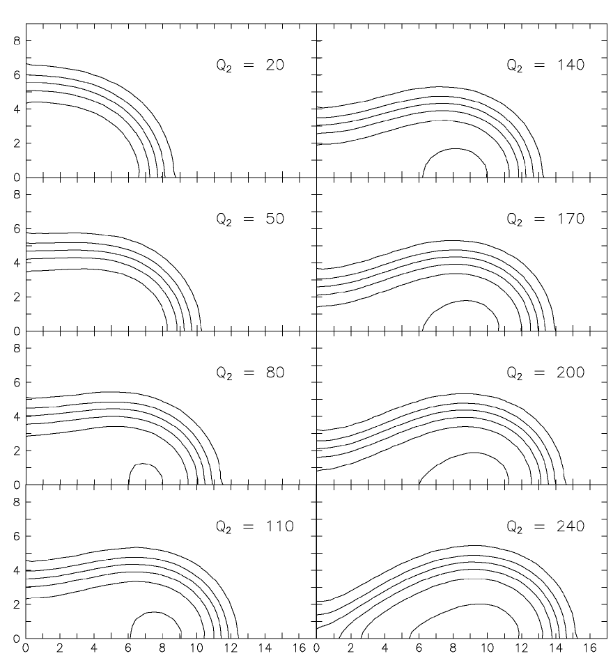
As stressed in [44] and [12, 45], in contrast to the liquid drop model, the HF formalism and its semiclassical version, Eq. (139), are capable to account for though small but finite compressibility of the nucleus. In order to illustrate this, consider the density distributions obtained in ETF calculations [46, 47] performed for 160Yb with a realistic Skyrme interaction, namely SkM∗ [23]. The function was taken in the form , with , , where are the Cartesian coordinates of . The collective coordinate for such a choice of has the meaning of the quadrupole moment . Since is invariant under rotations of about the axis, the densities are functions of , : . The values of , with , fm, along the fission path of 160Yb are depicted in Fig. 1. The profile function is defined as such contour on the , plot of , where . In Fig. 2 one can see those for the sequence of , presented in Fig. 1. Let be the volume of a body of constant density bound by the surface of revolution of about axis . From Fig. 3 one can see that this volume slightly decreases with elongation, which means that on its way to scission the nucleus is getting denser. Using the empirical formula (see Eq. (2.70) in [48])
for nuclear radii , we find that the ratio of the total volume of two spherical fission fragments to the volume of the spherical compound nucleus 160Yb is . This number is surprisingly close to the value from Fig. 3.
4.2 Inertia
By using (132), Eq. (56) for inertia may be rewritten as
| (140) |
where is the one-body operator with the matrix elements . Since , the inertia is expected to be expressible in terms of . The derivation of such an expression begins with using (129), (136) to represent (140) in the form
| (141) |
Here, is the single-particle Hamiltonian
with and
| (142) |
in accordance with (136), (138). In the subsequent discussion the term in is for simplicity omitted. Now, using the identity
| (143) |
we obtain
| (144) |
and
| (145) |
Next, replacing in (145) with in accordance with (49), we have
| (146) |
Substituting (146) into (141) and accounting for (136), we find the desired expression for :
| (147) |
where .
For calculating with the aid of (147) one should solve Eq. (50) for , which in the nuclei of complex shape is quite tedious. The well-known simplification consists in using the Werner-Wheeler approximation for . This approximation does not satisfy the condition , hence there is no Werner-Wheeler version of the phase function , to be used in (147). To circumvent this obstacle we express via the matrix elements of the one-body operator
| (148) |
Replacing in the right-hand side of (144) with , we find the formula
which allows to put Eq. (148) for into the form
from which, using (136), we find
| (149) |
Inserting (149) into Eq. (147), we arrive at the required expression for in terms of :
| (150) |
In order to use (150) in practical calculations, Eq. (148) for is rewritten in the form
| (151) |
with
| (152) |
and
| (153) |
where . The Latin indices represent the Cartesian components of the corresponding vector. The repeated indices are summed over from 1 to 3.
Following [29], consider a simplistic situation, when and are given by:
1) if is off the nuclear surface and if , where is an arbitrary point of the nuclear surface and is a unit vector normal to the surface at point ;
2) safely inside the nucleus, 0 safely outside of it, and is a step-like function of with vanishing width for close to the surface, where and is that point on the nuclear surface, which is the most close to .
It can be shown, using Eqs. (48), (151), (152), (153), that goes to in this case, so that given in (150) goes to
| (154) |
The index is designed to stress that Eq. (154), according to [31], follows from the cranking model formula for inertia of a Fermi gas [27], if any residual interaction is neglected. It can be shown analytically and numerically calculations [31] that as a function of is divergent near the crossing points of the single-particle energy levels, where . This signals that the simplistic situation considered in [29] is physically meaningless. Our derivation of (154) shows that could have been applicable for such a hypothetical nucleus, in which the mass flow induced by the distortion of the nuclear surface is getting immediately damped. This implies, of course, a very short mean free path, which is incompatible with the Fermi gas model of the nucleus used to derive (154).
The derivation of given in [27, 31] is based on the linear response theory. The fact that this theory leads to wrong inertia means that its application to nuclear collective motion is inappropriate. Really, the LRT regards such motion as a sequence of the states of complete thermal equilibrium at fixed nuclear shape. Within this simplistic picture there is no room for the mass flow in a hot time-evolving nucleus, which precludes the possibility for LRT to get the realistic estimates not only of collective inertia, but also of friction (see [35] for details).
In passing we note that some formally erroneous simplifications, destroying the self-consistency, need also to be made in deriving the cranking formula in cold nuclei from the adiabatic time-dependent Hartree-Fock theory (see Section 9.3 of [25] for details). Though the cranking model expression for the inertia in the dynamic equation for is wrong, the cranking model formulae for the inertia of the rotational and translational motions are correct. This is because the operators, which generate rotations and translations commute with the total Hamiltonian, while the operator of collective moment conjugated to does not.
4.3 Friction
Let , represent the creation and annihilation operators of quasiparticles with energies and wave functions , as found from Eqs. (136), (138). Substituting the expressions
| (155) |
into (126) and using (125), we find
| (156) |
where
For practical calculations of we take in the form
The Hamiltonian , which enters the propagators in , is modelled as
where
| (157) |
is the mean-field Hamiltonian, while is the residual interaction. The second equality in (157) is obtained by using (136), (155). The is given by
where
Let represent the collision time: , where is the range of the effective force and is the Fermi velocity. Then, following [49, 34], we postulate that for
| (158) |
where
| (159) |
with . Within perturbative treatment of , the collision rate of quasiparticles with nuclear media is related to the effective force as
| (160) |
where
The bold digits for quasi-particle quantum numbers are used to stress that the effective interaction in is not assumed to be diagonal over the spin-isospin quantum numbers . If does have this property,
and then if has the form
then becomes
The factor instead of the usual arises due to the fact that for the independent zero-range interaction the summation over , , is reduced to finding the sum
where is the spin-isospin exchange operator.
Eqs. (158), (159) imply that for the trajectory of any selected particle does not correlate with the trajectory of any selected hole, unless their quantum numbers coincide. Both the particle and the hole, however, have a chance to collide with nuclear media, which is reflected in the damping factors in Eq. (159) for their propagators. The simplest derivation of Eqs. (159), (160), not involving a diagrammatic expansion, but using instead Tserkovnikov’s substitution for and , can be found in [33]. In [34] we use a simple version of the effective force to obtain the semiclassical expression for in finite spherical nuclei and compare it to the values of in infinite matter.
The smallness of the collision time compared to the mean free path time , allows to use the asymptotic form (158), (159) of for all in (156), giving
where , . Then, we use the formula
to obtain
Noting that the factor in the summand is antisymmetric under interchange of with , we replace the remaining factor by its antisymmetric component
to obtain
| (161) |
where is an ’effective’ value of , not depending on the quantum numbers.
A seemingly different expression for follows from (123), if we replace there with , where , with defined in (148). The replacement of with is motivated by the assumption that is small and it leads to the quantity
| (162) |
From Eqs. (151), (152), ( 153) for it is seen that Eq. (162) coincides with the formula of Ref. [35]. Since the assumption on the smallness of implies that is small too, we may omit in the denominator of (162), which on accounting for Eq. (149) for leads to an expression for , which is identical to (161).
Comparing Eqs. (161) and (147) for and , respectively, we find the formula
| (163) |
which shows that the dependence of the reduced friction coefficient is completely determined by that of the collision rate defined in (160). For practical use of this expression we rewrite it as
| (164) |
where is the mean free path of the nucleon.
In Figs. 4, 5 the from (164) are superimposed on the semiclassical values of obtained from (162) in [35] by a conventional Monte-Carlo method. The calculation is done for 208Pb and 272Ds at , fm along the fission path starting from the spherical shape with the radius fm and ending at a necked-in configuration with the neck radius of 0.3. The given in (56) was calculated for 0.17 fm-3. For we took the distance between the mass centers of the two halves of the nucleus. The Werner-Wheeler expression for the ’fluid velocity’ and the Cassini oval parametrization for the profile function of the nuclear shape were used. One can see that does reproduce the general trends of as a function of , , and , although there are differences in detail. This may be related to the fact that the summand for is a sign-alternating function of the initial position and velocity of the particle, which makes the direct trajectory-integral simulations of unreliable (e.g. see [50]).
5 Summary and some remarks
The main objective of this study consists in working out a microscopic description of collective motion in hot nuclei, allowing to express the parameters of a phenomenological collective model [1, 2, 3] in terms of nucleonic quantities. The study starts with the introduction of the operator of collective coordinate and solving the two interwoven problems: construction of the quasiequilibrium density matrix and establishing the explicit expressions for the operators and of collective momentum conjugated to and collective inertia, respectively.
The crucial steps are: 1) the substitution , for the nucleon field operators made to get from the canonical density matrix subject to the condition and 2) the conversion of the adiabaticity hypothesis into assumption that the deviations of the number density and the momentum density , which are rapid functions of time, from their slow components and defined in (42) and (51), respectively, are smoothed out to a negligible level after performing the integrations invoked in the definitions of collective variables , , in terms of and .
Equating two different expressions for the time derivative of with then led us to a relation between the variation of collective velocity over the quasiequilibrium stage in question and a time integral over this stage of the function . After estimation of this integral in the adiabatic approximation, the relation takes the same form as the equation of motion of the phenomenological model, which allows us to identify the many-body expressions for collective inertia , deformation force , and friction coefficient .
Our microscopic expression , (56), for inertia has the form of inertia of collective motion in an abstract fluid with the velocity . It should be stressed that has nothing to do with the potential of the hydrodynamic velocity simply because this latter does not make sense in the nuclear case, once the nucleon mean free path is comparable or greater than the nuclear sizes. To the best of our knowledge this work is the first to derive the expression for the deformation force, where is the Lagrange multiplier used in the expression for to constrain it to a given expectation value of collective coordinate . Having shown that possesses the property , where is the free energy, we establish another expression for the deformation force: , which though used in some analyses of collective motion, has never been derived from first principles. Our microscopic expression for , (126), relating this quantity with the time integral of a time correlation function of for the ensemble, is also novel.
For practical calculations of , , and the real nucleus is replaced with a self-confined Fermi gas (SCFG) of quasiparticles, which, unlike the standard gases confined by external forces, is confined by its own forces. The SCFG model is based on the postulates that the one-body density matrix and the entropy of strongly-interacting nucleons, represented by have the same form as those of noninteracting fermions bound by an external one-body potential and that the expectation of the bare interparticle interaction for may be replaced with the expectation of the effective interaction for the two-body density matrix of noninteracting fermions. Use of the extreme property of Gibbs grand potential constructed within the SCFG model for the ensemble allows one to derive the temperature-dependent constrained Hartree-Fock equations with the effective interaction. These equations become especially simple when the effective interaction is the Skyrme force.
To find a SCFG expression for from Eq. (126), we assume independent decay of particle and hole states. Replacing for simplicity the decay width with the effective width not depending on quantum numbers, we arrive at the formula , where is the Fermi velocity, is the collective inertia, and the mean free path of the nucleon. According to this formula the , , and temperature dependences of the ratio are completely determined by those of . Perhaps this result will foster further analytical and computational studies of the nucleon mean free path in spherical, deformed, and superdeformed nuclei for realistic versions of the Skyrme force.
One of the principal results of this present paper and our previous work [35] is that they stress that the linear response theory (LRT) expressions for and [27, 28, 29, 30, 31, 32, 33, 34] are wrong. This is because the LRT is not applicable in the nuclear case. Namely, one cannot treat the force distorting the shape of a time evolving nucleus as an external force, because this force is depending on the intrinsic state of the nucleus. Moreover, the density matrix of the LRT implies that the mass flow in the bulk of the time-evolving nucleus is absent.
To understand the nature of nuclear collective motion it was important to realize a key role of the mass flow in this phenomenon and obtain an explicit expression for this quantity in a slowly evolving nucleus: if the equilibrium state of the nucleus is represented by the real-valued single-particle wave functions , for which the mass flow
then in the quasiequilibrium state of the nucleus those wave functions acquire the form , to give rise to a nonvanishing mass flow
where are the Fermi gas occupation numbers.
It is interesting to note that this way of generating the collective motion in hot nuclei is similar to generating the coherent motion in the entrance channel of the head-on nucleus-nucleus collision leading to the composite system under study (the total angular momentum of the nucleus is 0 in our model). Really, the ground states of two colliding nuclei can always be represented by superpositions of Slater determinants of single-particle standing waves. The relative motion with momentum in the head-on collision along the axis then gives rise to the phase factor attached to those standing waves with
where is the touching point. This new vision of mechanism of collective motion as manifestation of coherency of the phases of individual nucleons in the hot nucleus qualitatively differs from the N. Bohr picture of collective motion in fission [1], according to which the collective motion arises due to coherency of the velocities of individual nucleons.
Acknowledgements
The author is grateful to V.I. Abrosimov, M. Centelles, V.Yu. Denisov, S.N. Fedotkin, V.M. Kolomietz, V.A. Plujko, and A.I. Sanzhur for useful discussions.
Appendix A
In this appendix the operators , , , , , , , , , , are expressed in terms of the appropriate primed operators.
Using in (58), (60), we obtain
| (165) |
| (166) |
Eq. (59) for on accounting for (28), (48) takes the form
| (167) |
where
| (168) |
Eq. (89) for after accounting for (167), (166) takes the form
| (169) |
Eq. (52) for on accounting for (48), (168) becomes
| (170) |
Appendix B
Appendix C
Using the relation for and Eqs. (64), (79), (42), we find
| (179) |
This equation says that are linear functions of , which permits us to write , with . Thus, taking into account that , we obtain
From and (179) we find the expressions
| (180) |
where . Since , Eqs. (179), (180) show that are proportional to .
Appendix D
Let us prove that . Exploiting the cyclic property of the trace and definitions of , , and , we find that
valid for any c-number function , and Eq. (19), according to which , it is seen that , hence, . Analogously one shows that .
References
- [1] N. Bohr, J.A. Wheeler, Phys. Rev. 56 (1939) 426.
- [2] H.A. Kramers, Physica (Utrecht) 7 (1940) 284.
- [3] D.L. Hill, J.A. Wheeler, Phys. Rev. 89 (1953) 1102.
- [4] V.P. Aleshin, Nucl. Phys. A 605 (1996) 120.
- [5] P. Fröbrich, I.I. Gontchar, Physics Reports 292 (1998) 131.
- [6] E. G. Ryabov, A. V. Karpov, P. N. Nadtochy, G. D. Adeev, Phys. Rev. C 78, 044614 (2008) (15 pages)
- [7] A. Gavron, A. Gayer, J. Boissevain, H.C. Britt, T.C. Awes, J.R. Beene, B. Cheynis, D. Drain, R.L. Ferguson, F.E. Obenshain, F. Plasil, G.R. Young, G.A. Petitt, C. Butler, Phys. Rev. C 35 (1987) 579.
- [8] D.J. Hinde, D. Hilscher, H. Rossner, R. Gebauer, M. Lehmann, M. Wilpert, Phys. Rev. C 45 (1992) 1229.
- [9] J. Cabrera, Th. Keutgen, Y. El Masri, Ch. Dufauquez, V. Roberfroid, I. Tilquin, J. Van Mol, R. Régimbart, R. J. Charity, J. B. Natowitz, K. Hagel, R. Wada, D. J. Hinde, Phys. Rev. C 68, 034613 (2003) (21 pages)
- [10] R. Rafiei, R. G. Thomas, D. J. Hinde, M. Dasgupta, C. R. Morton, L. R. Gasques, M. L. Brown, M. D. Rodriguez, Phys. Rev. C 77, 024606 (2008) (9 pages)
- [11] V.M. Strutinsky, N.Ya. Lyashchenko, N.A. Popov, Zh. Eksp. Teor. Fiz. 43 (1962) 584; Nucl. Phys. 46 (1963) 639.
- [12] V.M. Strutinsky, A.S. Tyapin, Zh. Eksp. Teor. Fiz. 45 (1963) 960.
- [13] P. Quentin, H. Flocard, Ann. Rev. Nucl. Part. Sci. 28 (1978) 523.
- [14] T.H.R. Skyrme, Nucl. Phys. 9 (1959) 615.
- [15] D. Vautherin, D.M. Brink, Phys. Rev. C5 (1972) 626.
- [16] D. Vautherin, Phys. Rev. C7 (1973) 196.
- [17] M. Bender, P.-H. Heenen, P.-G. Reinhard, Rev. Mod. Phys. 75 (2003) 121.
- [18] J. Dechargé, D. Gogny, Phys. Rev. C 21 (1980) 1568.
- [19] B.D. Serot, J. D. Walecka, Adv. Nucl. Phys. 16 (1986) 1.
- [20] J.W. Negele, in: G. Ripka, M. Porneuf (Eds.) Nuclear Self-Consistent Fields, North-Holland, Amsterdam, 1975, p. 113.
- [21] H. Flocard, P. Quentin, D. Vautherin, M. Vénéroni, A.K. Kerman, Nucl. Phys. A 231 (1974) 176.
- [22] M. Brack, J. Damgaard, A.S. Jensen, H.C. Pauli, V.M. Strutinsky, C.Y. Wong, Reviews of Modern Physics, 44 no.2 (1972) 320.
- [23] M. Brack, C. Guet, H.-B. Hakansson, Phys. Rep. 123, No. 5 (1985) 276.
- [24] P. Villars, in: G. Ripka, M. Porneuf (Eds.) Nuclear Self-Consistent Fields, North-Holland, Amsterdam, 1975, p. 3.
- [25] M. Baranger, M. Veneroni, Ann. Phys. 114, no. 1 (1978) 123.
- [26] B.I. Bartz, Yu.L. Bolotin, E.B. Inopin, V.Yu. Gonchar, Hartree-Fock Method in Nuclear Theory, Naukova Dumka, Kiev, 1982, pp. 165-199 (in Russian).
- [27] H. Hofmann, Phys. Lett. 61 B, no. 5 (1976) 423.
- [28] S.E. Koonin, R.L. Hatch, J.R. Ranrup, Nucl. Phys. A283 (1977) 87.
- [29] S.E. Koonin, J. Randrup, Nucl. Phys. A289 (1977) 475.
- [30] V.M. Kolomietz, Izv. Akad Nauk SSSR (Ser. Fiz.) 42 (1978) 1851.
- [31] S. Yamaji, H. Hofmann, R. Samhammer, Nucl. Phys. A 475 (1988) 487.
- [32] V.P. Aleshin, Acta Phys. Pol. 30 (3) (1999) 461.
- [33] V.P. Aleshin, Ukr. J. Phys. 48 (5) (2003) 486.
- [34] V.P. Aleshin, Nucl. Phys. A 760 (2005) 234.
- [35] V.P. Aleshin, Nucl. Phys. A 781 (2007) 363.
- [36] E.T. Jaynes, Phys. Rev. 106 (1957) 620.
- [37] R. Balian, C. de Dominicis, Ann. Phys. 62 no. 1 (1971) 229.
- [38] H. Umezawa, H. Matsumoto, M. Tachiki, Thermo Field Dynamics and Condensed States, North-Holland, Amsterdam, 1982.
- [39] J. von Neumann, Mathematical Foundations of Quantum Mechanics, Princeton University Press, Princeton, 1955, Chap. 5, Sec. 3.
- [40] N.D. Mermin, Phys. Rev. 137 (1965) A1441.
- [41] H. Mori, Phys. Rev. 112 (1958) 1829.
- [42] A.I. Akhiezer, C.B. Peletminsky, Methods of Statistical Physics, Nauka, Moskva (1977) pp. 199-200 (in Russian)
- [43] M. Brack, R.K. Bhadury, Semiclassical Physics, Addison-Wesley, Reading, MA, 2003.
- [44] H. Flocard, P. Quentin, D. Vautherin, M. Vénéroni, A.K. Kerman, Nucl. Phys. A 231 (1974) 176.
- [45] A.S. Tyapin, Yad. Fiz., 13 (1) (1971) 32.
- [46] V.P. Aleshin, B. Sidorenko, M. Centelles, X. Vinas, Acta Phys. Pol. B 28 (1997) 387.
- [47] V.P. Aleshin, M. Centelles, X. Vinas, N.G. Nicolis, Nucl. Phys. A 679 (2001) 441.
- [48] A. Bohr, B.R. Mottelson, Nuclear Structure, Volume 1, Benjamin, New York, 1969.
- [49] P.J. Siemens, A.S. Jensen, H. Hofmann, Nucl. Phys. A 441 (1985) 410.
- [50] C.H. Mak, D. Chandler, Phys. Rev. A44, no. 4 (1991) 2352.