Polaron Properties of an Impurity in Bose-Einstein-Condensation

Beibing Huang and Shaolong Wan
Institute for Theoretical Physics and Department of Modern Physics
University of Science and Technology of China, Hefei, 230026, P. R. China
Corresponding author. Electronic address: slwan@ustc.edu.cn

Abstract

In this paper we study an impurity in Bose-Einstein-Condensate system at $T=0K$ and suppose the contact forms for boson-boson and boson-impurity interactions. Using Bogoliubov theory and a further approximation corresponding to only think over the forward scattering of impurity by bosons, we derive a reduced Hamiltonian whose form is the same as the FrΓΆhlich Hamiltonian for large polaron. By using Lee-Low-Pines (LLP) theory for large polaron, we obtain the effective mass of impurity, the phonon number carried by impurity and the energy related to the existence of impurity. In addition, we also discuss the valid range for forward-scattering approximation.


PACS number(s): 03.75.Kk, 03.75.Ss, 74.20.Mn

1 Introduction

Since the impressive experimental achievement of Bose-Einstein-Condensation (BEC) [1, 2, 3] quantum degenerate atomic gases have become one of the hottest domains. Temperature in such systems can be thought to approach zero so that the thermal fluctuations and classical phase transitions associated with thermal fluctuations are fully suppressed. But quantum fluctuations due to Heisenberg uncertainty principle still exist and may be strong enough to lead to a quantum phase transition. So these systems are good playground to realization of quantum phase transitions [4, 5, 6]. Except probing for fundamental physics in the realm of dilute atomic quantum gas, BEC system is also an auxiliary but effective tool to sympathetically cool some systems, which can not be cooled by traditional cooling technique, to degenerate temperature [7, 8, 9]. So a quantum degenerate mixing system could be obtained. Extending such mixing system to a extreme case that there is only one atom belonging to sympathetically cooled system, we will expect a BEC system with an impurity. Fortunately, such system has been able to create in experiment by many ways [9, 10, 11, 12]. An impurity in BEC is very similar to polaron, an electron in ionic crystal. When the electron moves, it polarizes the lattice around it and inversely experiences an effective potential from the lattice. And in the BEC system, the existence of an impurity would modify the distribution of atoms in BEC and also produce an effective potential to act on itself [13]. In [13, 14, 15], their authors made good use of the product wave function similar to Landau-Pekar description to polaron [16, 17] to deal with the self-localization of impurity. The product wave function, the essence of which is the separation of freedoms, is a good approximation for polaron owing to large mass ratio of ion to the electron to make the Born-Oppenheimer approximation be valid. But the validity of product wave function is questionable in the BEC system with an impurity, owing to similar masses between the bosons and the impurity, and some deviations from it can be expected [15].

In this article, we start from the bosonic system Hamiltonian with an impurity, and by using Bogoliubov theory, derive an equivalent Hamiltonian which is the same as the FrΓΆhlich Hamiltonian [18, 19] for large polaron in section 2. In this equivalent Hamiltonian, Bogoliubov phonon plays a role of the phonon which comes from the lattice oscillation. Then we use intermediate coupling theory [20] of Lee-Low-Pines (LLP) for polaron to calculate the effective mass of impurity, the phonon number carried by impurity and the impurity energy in section 3. Finally, some discussions about validity of our approximate decision on condensate fraction and conclusions are given in section 4.

2 Equivalent Hamiltonian for the Bosonic System with an Impurity

We consider a single impurity immersed in a homogeneous BEC in three dimension space. Assuming that the boson-boson and boson-impurity interactions can be described by contact interactions, the many-body Hamiltonian [14] reads

$\displaystyle H$ $\displaystyle=$ $\displaystyle-\sum_{i}\frac{\hbar^{2}\bigtriangledown_{i}^{2}}{2m_{B}}+\frac{g}{2}\sum_{i,j}\delta(\vec{r}_{i}-\vec{r}_{j})$ (1)
$\displaystyle+\lambda\sum_{i}\delta(\vec{r}-\vec{r}_{i})-\frac{\hbar^{2}\bigtriangledown^{2}}{2m_{I}}$

where $m_{B}$, $m_{I}$ are the masses of boson and impurity respectively. $g=4\pi\hbar^{2}a_{BB}/m_{B}$, $\lambda=2\pi\hbar^{2}a_{IB}/m_{red}$ are the interaction strength of contact potentials for boson-boson and boson-impurity interaction with the reduced mass $m_{red}=m_{I}m_{B}/(m_{I}+m_{B})$. $\vec{r}_{i}$, $\vec{r}$ represent the coordinates of bosons and impurity, respectively. In the second quantization representation, we can expand the bosonic field operator on a set of plane wave basis and change Hamiltonian (1) into

$\displaystyle H$ $\displaystyle=$ βˆ‘k(Ξ΅kβˆ’ΞΌ)​ak†​ak+g2β€‹βˆ‘k,p,qak†​ap†​apβˆ’q​ak+qsubscriptπ‘˜subscriptπœ€π‘˜πœ‡superscriptsubscriptπ‘Žπ‘˜β€ subscriptπ‘Žπ‘˜π‘”2subscriptπ‘˜π‘π‘žsuperscriptsubscriptπ‘Žπ‘˜β€ superscriptsubscriptπ‘Žπ‘β€ subscriptπ‘Žπ‘π‘žsubscriptπ‘Žπ‘˜π‘ž\displaystyle\sum_{k}(\varepsilon_{k}-\mu)a_{k}^{{\dagger}}a_{k}+\frac{g}{2}\sum_{k,p,q}a_{k}^{{\dagger}}a_{p}^{{\dagger}}a_{p-q}a_{k+q} (2)
+Ξ»β€‹βˆ‘k,qak†​aq​exp⁑[βˆ’i​(kβ†’βˆ’qβ†’)β‹…rβ†’]+P22​mIπœ†subscriptπ‘˜π‘žsuperscriptsubscriptπ‘Žπ‘˜β€ subscriptπ‘Žπ‘žβ‹…π‘–β†’π‘˜β†’π‘žβ†’π‘Ÿsuperscript𝑃22subscriptπ‘šπΌ\displaystyle+\lambda\sum_{k,q}a_{k}^{{\dagger}}a_{q}\exp\left[-i(\vec{k}-\vec{q})\cdot\vec{r}\right]+\frac{P^{2}}{2m_{I}}

where $\varepsilon_{k}=\hbar^{2}k^{2}/(2m_{B})$ and $\vec{P}$ is the momentum of impurity. The chemical potential $\mu$ is introduced to keep the average bosonic number to be a constant. ak,ak†subscriptπ‘Žπ‘˜superscriptsubscriptπ‘Žπ‘˜β€ a_{k},a_{k}^{{\dagger}} are the bosonic annihilation and creation operators conforming to the canonical commutation relation [ak,aq†]=Ξ΄k​qsubscriptπ‘Žπ‘˜superscriptsubscriptπ‘Žπ‘žβ€ subscriptπ›Ώπ‘˜π‘ž[a_{k},a_{q}^{{\dagger}}]=\delta_{kq}. Owing to only one impurity, the statistical property of impurity is unimportant and the same results are obtained for the fermionic and bosonic impurity. For the convenience, we suppose our system to be unit volume.

At $T=0K$, the bosons macroscopically occupy the lowest energy state with wave vector $\vec{k}=0$, which makes it possible to neglect quantum property of $a_{0},a_{0}^{{\dagger}}$ and consider them to be classical number [21]. Following the general procedure, we decompose $a_{k}$ as follows

$\displaystyle a_{k}\rightarrow\sqrt{n_{0}}\delta_{k0}+a_{k}$ (3)

$n_{0}$ is the number density of atom on the lowest energy state with $n_{0}=a_{0}^{{\dagger}}a_{0}$. Substituting (3) into (2) and only keeping terms until the second order, the Hamiltonian reads

$\displaystyle H$ $\displaystyle=$ $\displaystyle\frac{P^{2}}{2m_{I}}-\mu n_{0}+\frac{g}{2}n_{0}^{2}+\lambda n_{0}+\sqrt{n_{0}}(-\mu+gn_{0}+\lambda)(a_{0}+a_{0}^{{\dagger}})$ (4)
+λ​n0β€‹βˆ‘kβ€²[ak​exp⁑(i​kβ†’β‹…rβ†’)+ak†​exp⁑(βˆ’i​kβ†’β‹…rβ†’)]+Ξ»β€‹βˆ‘k,qak†​aq​exp⁑[βˆ’i​(kβ†’βˆ’qβ†’)β‹…rβ†’]πœ†subscript𝑛0superscriptsubscriptπ‘˜β€²delimited-[]subscriptπ‘Žπ‘˜β‹…π‘–β†’π‘˜β†’π‘Ÿsuperscriptsubscriptπ‘Žπ‘˜β€ β‹…π‘–β†’π‘˜β†’π‘Ÿπœ†subscriptπ‘˜π‘žsuperscriptsubscriptπ‘Žπ‘˜β€ subscriptπ‘Žπ‘žβ‹…π‘–β†’π‘˜β†’π‘žβ†’π‘Ÿ\displaystyle+\lambda\sqrt{n_{0}}\sum_{k}^{{}^{\prime}}\left[a_{k}\exp(i\vec{k}\cdot\vec{r})+a_{k}^{{\dagger}}\exp(-i\vec{k}\cdot\vec{r})\right]+\lambda\sum_{k,q}a_{k}^{{\dagger}}a_{q}\exp[-i(\vec{k}-\vec{q})\cdot\vec{r}]
+βˆ‘k(Ξ΅kβˆ’ΞΌ)​ak†​ak+g​n02β€‹βˆ‘k(ak​aβˆ’k+4​ak†​ak+ak†​aβˆ’k†)subscriptπ‘˜subscriptπœ€π‘˜πœ‡superscriptsubscriptπ‘Žπ‘˜β€ subscriptπ‘Žπ‘˜π‘”subscript𝑛02subscriptπ‘˜subscriptπ‘Žπ‘˜subscriptπ‘Žπ‘˜4superscriptsubscriptπ‘Žπ‘˜β€ subscriptπ‘Žπ‘˜superscriptsubscriptπ‘Žπ‘˜β€ superscriptsubscriptπ‘Žπ‘˜β€ \displaystyle+\sum_{k}(\varepsilon_{k}-\mu)a_{k}^{{\dagger}}a_{k}+\frac{gn_{0}}{2}\sum_{k}(a_{k}a_{-k}+4a_{k}^{{\dagger}}a_{k}+a_{k}^{{\dagger}}a_{-k}^{{\dagger}})

where the sum with character $\sum_{k}^{{}^{\prime}}$ represents exclusion for $\vec{k}=0$ state. Note that both interactions of boson-boson and boson-impurity make the BEC deplete. We take into consideration contributions of such two kinds of interaction to the condensate depletion at the same time by asking for the coefficient of $a_{0},a_{0}^{{\dagger}}$ to vanish [21] and find

$\displaystyle\mu=gn_{0}+\lambda$ (5)

When BEC happens, the gauge symmetry of the system is broken and a long-wavelength gapless mode exists which is imposed by Goldstone theorem [22]. In order to satisfy above condition, we find that if we make below approximation for boson-impurity scattering term

Ξ»β€‹βˆ‘k,qak†​aq​exp⁑[βˆ’i​(kβ†’βˆ’qβ†’)β‹…rβ†’]β‰ˆΞ»β€‹βˆ‘kak†​akπœ†subscriptπ‘˜π‘žsuperscriptsubscriptπ‘Žπ‘˜β€ subscriptπ‘Žπ‘žβ‹…π‘–β†’π‘˜β†’π‘žβ†’π‘Ÿπœ†subscriptπ‘˜superscriptsubscriptπ‘Žπ‘˜β€ subscriptπ‘Žπ‘˜\displaystyle\lambda\sum_{k,q}a_{k}^{{\dagger}}a_{q}\exp{[-i(\vec{k}-\vec{q})\cdot\vec{r}]}\approx\lambda\sum_{k}a_{k}^{{\dagger}}a_{k} (6)

the gapless property of low energy excitations is met as we could see below. Physically this approximation implies that when the impurity is scattered by bosons, the momentum of bosons and impurity will not alter. In other words, impurity only experiences forward scattering. So the Hamiltonian is further reduced to

$\displaystyle H$ $\displaystyle=$ $\displaystyle\frac{P^{2}}{2m_{I}}-\frac{g}{2}n_{0}^{2}-\frac{1}{2}\sum_{k}(\varepsilon_{k}+gn_{0})$ (7)
+λ​n0β€‹βˆ‘kβ€²[ak​exp⁑(i​kβ†’β‹…rβ†’)+ak†​exp⁑(βˆ’i​kβ†’β‹…rβ†’)]πœ†subscript𝑛0superscriptsubscriptπ‘˜β€²delimited-[]subscriptπ‘Žπ‘˜β‹…π‘–β†’π‘˜β†’π‘Ÿsuperscriptsubscriptπ‘Žπ‘˜β€ β‹…π‘–β†’π‘˜β†’π‘Ÿ\displaystyle+\lambda\sqrt{n_{0}}\sum_{k}^{{}^{\prime}}\left[a_{k}\exp{(i\vec{k}\cdot\vec{r})}+a_{k}^{{\dagger}}\exp{(-i\vec{k}\cdot\vec{r})}\right]
+12β€‹βˆ‘k(Ξ΅k+g​n0)​(ak†​ak+aβˆ’k​aβˆ’k†)12subscriptπ‘˜subscriptπœ€π‘˜π‘”subscript𝑛0superscriptsubscriptπ‘Žπ‘˜β€ subscriptπ‘Žπ‘˜subscriptπ‘Žπ‘˜superscriptsubscriptπ‘Žπ‘˜β€ \displaystyle+\frac{1}{2}\sum_{k}(\varepsilon_{k}+gn_{0})(a_{k}^{{\dagger}}a_{k}+a_{-k}a_{-k}^{{\dagger}})
+g​n0​(ak​aβˆ’k+ak†​aβˆ’k†)𝑔subscript𝑛0subscriptπ‘Žπ‘˜subscriptπ‘Žπ‘˜superscriptsubscriptπ‘Žπ‘˜β€ superscriptsubscriptπ‘Žπ‘˜β€ \displaystyle+gn_{0}(a_{k}a_{-k}+a_{k}^{{\dagger}}a_{-k}^{{\dagger}})

Making the Bogoliubov transformation

$\displaystyle a_{k}$ $\displaystyle=$ uk​bkβˆ’vk​bβˆ’k†subscriptπ‘’π‘˜subscriptπ‘π‘˜subscriptπ‘£π‘˜superscriptsubscriptπ‘π‘˜β€ \displaystyle u_{k}b_{k}-v_{k}b_{-k}^{{\dagger}}
aβˆ’k†superscriptsubscriptπ‘Žπ‘˜β€ \displaystyle a_{-k}^{{\dagger}} $\displaystyle=$ βˆ’vk​bk+uk​bβˆ’k†subscriptπ‘£π‘˜subscriptπ‘π‘˜subscriptπ‘’π‘˜superscriptsubscriptπ‘π‘˜β€ \displaystyle-v_{k}b_{k}+u_{k}b_{-k}^{{\dagger}} (8)

and imposing the conditions

$\displaystyle u_{k}^{2}-v_{k}^{2}=1$
$\displaystyle(u_{k}^{2}+v_{k}^{2})gn_{0}-2u_{k}v_{k}(gn_{0}+\varepsilon_{k})=0$
$\displaystyle\xi_{k}=(u_{k}^{2}+v_{k}^{2})(\varepsilon_{k}+gn_{0})-2u_{k}v_{k}gn_{0}$ (9)

We obtain

$\displaystyle H$ $\displaystyle=$ EB+P22​mI+βˆ‘kΞΎk​bk†​bksubscript𝐸𝐡superscript𝑃22subscriptπ‘šπΌsubscriptπ‘˜subscriptπœ‰π‘˜superscriptsubscriptπ‘π‘˜β€ subscriptπ‘π‘˜\displaystyle E_{B}+\frac{P^{2}}{2m_{I}}+\sum_{k}\xi_{k}b_{k}^{{\dagger}}b_{k} (10)
$\displaystyle+$ βˆ‘kβ€²[Vk​bk​exp⁑(i​kβ†’β‹…rβ†’)+Vkβˆ—β€‹bk†​exp⁑(βˆ’i​kβ†’β‹…rβ†’)]superscriptsubscriptπ‘˜β€²delimited-[]subscriptπ‘‰π‘˜subscriptπ‘π‘˜β‹…π‘–β†’π‘˜β†’π‘Ÿsuperscriptsubscriptπ‘‰π‘˜βˆ—superscriptsubscriptπ‘π‘˜β€ β‹…π‘–β†’π‘˜β†’π‘Ÿ\displaystyle\sum_{k}^{{}^{\prime}}\left[V_{k}b_{k}\exp{(i\vec{k}\cdot\vec{r})}+V_{k}^{\ast}b_{k}^{{\dagger}}\exp{(-i\vec{k}\cdot\vec{r})}\right]

where $V_{k}=\lambda\sqrt{n_{0}}(u_{k}-v_{k})$ and $E_{B}=-\frac{g}{2}n_{0}^{2}+\frac{1}{2}\sum_{k}(\xi_{k}-\varepsilon_{k}-gn_{0})$. $\xi_{k}=\sqrt{\varepsilon_{k}^{2}+2gn_{0}\varepsilon_{k}}$ with $v_{k}^{2}=u_{k}^{2}-1=\frac{1}{2}(\frac{\varepsilon_{k}+gn_{0}}{\xi_{k}}-1),u_{k}v_{k}=\frac{gn_{0}}{2\xi_{k}}$. It is very clear that low energy excitation $\xi_{k}$ is gapless and completely same as that in the situation without the impurity. $n_{0}$ is decided by atomic number conservation

$\displaystyle n$ $\displaystyle=$ n0+βˆ‘k<ak†​ak>subscript𝑛0subscriptπ‘˜expectationsuperscriptsubscriptπ‘Žπ‘˜β€ subscriptπ‘Žπ‘˜\displaystyle n_{0}+\sum_{k}<a_{k}^{{\dagger}}a_{k}> (11)
$\displaystyle=$ n0+βˆ‘kvk2+βˆ‘k(uk2+vk2)​<bk†​bk>βˆ’βˆ‘kuk​vk​<bk†​bβˆ’k†+bk​bβˆ’k>subscript𝑛0subscriptπ‘˜superscriptsubscriptπ‘£π‘˜2subscriptπ‘˜superscriptsubscriptπ‘’π‘˜2superscriptsubscriptπ‘£π‘˜2expectationsuperscriptsubscriptπ‘π‘˜β€ subscriptπ‘π‘˜subscriptπ‘˜subscriptπ‘’π‘˜subscriptπ‘£π‘˜expectationsuperscriptsubscriptπ‘π‘˜β€ superscriptsubscriptπ‘π‘˜β€ subscriptπ‘π‘˜subscriptπ‘π‘˜\displaystyle n_{0}+\sum_{k}v_{k}^{2}+\sum_{k}(u_{k}^{2}+v_{k}^{2})<b_{k}^{{\dagger}}b_{k}>-\sum_{k}u_{k}v_{k}<b_{k}^{{\dagger}}b_{-k}^{{\dagger}}+b_{k}b_{-k}>

Where $<\cdots>$ represents the ensemble average. In the pure bosonic system, Bogoliubov transformation makes the Hamiltonian of bosonic system diagonal about phonon operators, so the last two terms on the right hand side disappear and $n_{0}$ is decided by equation

$\displaystyle n=n_{0}+\sum_{k}v_{k}^{2}$ (12)

While for the bosonic system with an impurity the last two terms are nonzero, leading to that the particle number equation and bosonic condensate fraction are modified in contrast to pure bosonic system. In fact, the last two terms in (11) illustrate the contribution of impurity to condensate depletion. But as we will see below, the last two terms are much smaller than other terms in (11) and are negligible due to small ratio of impurity number to boson number. Thus, we determine condensate fraction according to (12), in other words, we do not consider the contribution of boson-impurity interaction to condensate depletion. When $n_{0}$ is determined, the Hamiltonian (10) is completely decided.

Owing to nonexistence of zero-momentum phonon, exclusion for $\vec{k}=0$ state in (10) is not important and we can neglect this exclusion. In addition to a constant term $E_{B}$, the form of Hamiltonian (10) is the same as that of FrΓΆhlich large polaron theory. Bogoliubov phonon is akin to phonon coming from lattice oscillations. When an electron moves in ionic crystal, it will be influenced more strongly by optical phonon, which represents relative movement of positive and negative ions and is accompanied by polarized electric field, than acoustic one which represents the movement of mass center and can not produce polarized electric field. So in usual FrΓΆhlich large polaron theory, the phonon is considered to be optical mode one and its frequency is chosen to be independent of the wavevector and be a nonzero constant due to finite energy gap for optical phonon. But in BEC system with an impurity phonon is gapless, moreover we must consider the dependence of dispersion relation on wavevector. As a summarization of this section, we get an effective Hamiltonian similar to FrΓΆhlich large polaron by making Bogoliubov and forward-scattering approximations.

3 The Effective Mass, Phonon Number and Impurity Energy

Below, we follow the LLP approach [20] to calculate some properties of such system. The essence of the LLP theory consists in combining the canonical transformation with the variational principle to get approximate ground state of the system. Supposing $|\Phi>$ is the ground state $H|\Phi>=E|\Phi>$, we make the canonical transformation $|\Phi>=U_{1}|\Psi>$ with U1=exp⁑[βˆ’iβ€‹βˆ‘kbk†​bk​kβ†’β‹…rβ†’]subscriptπ‘ˆ1𝑖subscriptπ‘˜β‹…superscriptsubscriptπ‘π‘˜β€ subscriptπ‘π‘˜β†’π‘˜β†’π‘ŸU_{1}=\exp{[-i\sum_{k}b_{k}^{{\dagger}}b_{k}\vec{k}\cdot\vec{r}]} and the Hamiltonian is transformed into $H^{{}^{\prime}}=U_{1}^{-1}HU_{1}$

$\displaystyle H^{{}^{\prime}}$ $\displaystyle=$ EB+(Pβ†’βˆ’βˆ‘kℏ​k→​bk†​bk)22​mIsubscript𝐸𝐡superscript→𝑃subscriptπ‘˜Planck-constant-over-2-piβ†’π‘˜superscriptsubscriptπ‘π‘˜β€ subscriptπ‘π‘˜22subscriptπ‘šπΌ\displaystyle E_{B}+\frac{(\vec{P}-\sum_{k}\hbar\vec{k}b_{k}^{{\dagger}}b_{k})^{2}}{2m_{I}} (13)
+βˆ‘kΞΎk​bk†​bk+βˆ‘k(Vk​bk+Vkβˆ—β€‹bk†)subscriptπ‘˜subscriptπœ‰π‘˜superscriptsubscriptπ‘π‘˜β€ subscriptπ‘π‘˜subscriptπ‘˜subscriptπ‘‰π‘˜subscriptπ‘π‘˜superscriptsubscriptπ‘‰π‘˜βˆ—superscriptsubscriptπ‘π‘˜β€ \displaystyle+\sum_{k}\xi_{k}b_{k}^{{\dagger}}b_{k}+\sum_{k}(V_{k}b_{k}+V_{k}^{\ast}b_{k}^{{\dagger}})

In (13), the coordinate of impurity is expunged and its momentum becomes a good quantum number. In fact, the momentum $\vec{P}$ in (13) represents the whole momentum of the system. Introducing the variational function $f(k)$ and making another canonical transformation $|\Psi>=U_{2}|0>$ with U2=exp⁑[βˆ‘k(bk†​f​(k)βˆ’bk​fβˆ—β€‹(k))]subscriptπ‘ˆ2subscriptπ‘˜superscriptsubscriptπ‘π‘˜β€ π‘“π‘˜subscriptπ‘π‘˜superscriptπ‘“βˆ—π‘˜U_{2}=\exp{[\sum_{k}(b_{k}^{{\dagger}}f(k)-b_{k}f^{\ast}(k))]} and $|0>$ representing the vacuum of the phonon, the Hamiltonian (13) can be rewritten as $\widehat{H}=U_{2}^{-1}H^{{}^{\prime}}U_{2}$

$\displaystyle\widehat{H}$ $\displaystyle=$ EB+(Pβ†’βˆ’βˆ‘kℏ​k→​bk†​bk)22​mI+βˆ‘k[Vk​f​(k)+Vkβˆ—β€‹fβˆ—β€‹(k)]+ℏ22​mIβ€‹βˆ‘k,qkβ†’β‹…q→​|f​(k)|2​|f​(q)|2subscript𝐸𝐡superscript→𝑃subscriptπ‘˜Planck-constant-over-2-piβ†’π‘˜superscriptsubscriptπ‘π‘˜β€ subscriptπ‘π‘˜22subscriptπ‘šπΌsubscriptπ‘˜delimited-[]subscriptπ‘‰π‘˜π‘“π‘˜superscriptsubscriptπ‘‰π‘˜βˆ—superscriptπ‘“βˆ—π‘˜superscriptPlanck-constant-over-2-pi22subscriptπ‘šπΌsubscriptπ‘˜π‘žβ‹…β†’π‘˜β†’π‘žsuperscriptπ‘“π‘˜2superscriptπ‘“π‘ž2\displaystyle E_{B}+\frac{(\vec{P}-\sum_{k}\hbar\vec{k}b_{k}^{{\dagger}}b_{k})^{2}}{2m_{I}}+\sum_{k}\left[V_{k}f(k)+V_{k}^{\ast}f^{\ast}(k)\right]+\frac{\hbar^{2}}{2m_{I}}\sum_{k,q}\vec{k}\cdot\vec{q}|f(k)|^{2}|f(q)|^{2} (14)
$\displaystyle+$ βˆ‘k|f​(k)|2​[Ο΅kβˆ’β„mI​Pβ†’β‹…kβ†’+ΞΎk]+βˆ‘kΞΎk​bk†​bk+βˆ‘kbk†​bkβ€‹βˆ‘qℏ2mI​kβ†’β‹…q→​|f​(q)|2subscriptπ‘˜superscriptπ‘“π‘˜2delimited-[]subscriptitalic-Ο΅π‘˜β‹…Planck-constant-over-2-pisubscriptπ‘šπΌβ†’π‘ƒβ†’π‘˜subscriptπœ‰π‘˜subscriptπ‘˜subscriptπœ‰π‘˜superscriptsubscriptπ‘π‘˜β€ subscriptπ‘π‘˜subscriptπ‘˜superscriptsubscriptπ‘π‘˜β€ subscriptπ‘π‘˜subscriptπ‘žβ‹…superscriptPlanck-constant-over-2-pi2subscriptπ‘šπΌβ†’π‘˜β†’π‘žsuperscriptπ‘“π‘ž2\displaystyle\sum_{k}|f(k)|^{2}\left[\epsilon_{k}-\frac{\hbar}{m_{I}}\vec{P}\cdot\vec{k}+\xi_{k}\right]+\sum_{k}\xi_{k}b_{k}^{{\dagger}}b_{k}+\sum_{k}b_{k}^{{\dagger}}b_{k}\sum_{q}\frac{\hbar^{2}}{m_{I}}\vec{k}\cdot\vec{q}|f(q)|^{2}
$\displaystyle+$ $\displaystyle\sum_{k}\left\{b_{k}^{{\dagger}}\left[V_{k}^{\star}+f(k)\left(\xi_{k}+\epsilon_{k}-\frac{\hbar}{m_{I}}\vec{P}\cdot\vec{k}+\frac{\hbar^{2}}{m_{I}}\sum_{q}\vec{k}\cdot\vec{q}|f(q)|^{2}\right)\right]+h.c.\right\}$
$\displaystyle+$ ℏ22​mIβ€‹βˆ‘k,qkβ†’β‹…q→​[bk†​bq†​f​(k)​f​(q)+2​bk†​bq​f​(k)​fβˆ—β€‹(q)+bk​bq​fβˆ—β€‹(k)​fβˆ—β€‹(q)]superscriptPlanck-constant-over-2-pi22subscriptπ‘šπΌsubscriptπ‘˜π‘žβ‹…β†’π‘˜β†’π‘ždelimited-[]superscriptsubscriptπ‘π‘˜β€ superscriptsubscriptπ‘π‘žβ€ π‘“π‘˜π‘“π‘ž2superscriptsubscriptπ‘π‘˜β€ subscriptπ‘π‘žπ‘“π‘˜superscriptπ‘“βˆ—π‘žsubscriptπ‘π‘˜subscriptπ‘π‘žsuperscriptπ‘“βˆ—π‘˜superscriptπ‘“βˆ—π‘ž\displaystyle\frac{\hbar^{2}}{2m_{I}}\sum_{k,q}\vec{k}\cdot\vec{q}\left[b_{k}^{{\dagger}}b_{q}^{{\dagger}}f(k)f(q)+2b_{k}^{{\dagger}}b_{q}f(k)f^{\ast}(q)+b_{k}b_{q}f^{\ast}(k)f^{\ast}(q)\right]
$\displaystyle+$ ℏ2mIβ€‹βˆ‘k,qkβ†’β‹…q→​[fβˆ—β€‹(q)​bk†​bk​bq+f​(q)​bq†​bk†​bk]superscriptPlanck-constant-over-2-pi2subscriptπ‘šπΌsubscriptπ‘˜π‘žβ‹…β†’π‘˜β†’π‘ždelimited-[]superscriptπ‘“βˆ—π‘žsuperscriptsubscriptπ‘π‘˜β€ subscriptπ‘π‘˜subscriptπ‘π‘žπ‘“π‘žsuperscriptsubscriptπ‘π‘žβ€ superscriptsubscriptπ‘π‘˜β€ subscriptπ‘π‘˜\displaystyle\frac{\hbar^{2}}{m_{I}}\sum_{k,q}\vec{k}\cdot\vec{q}\left[f^{\ast}(q)b_{k}^{{\dagger}}b_{k}b_{q}+f(q)b_{q}^{{\dagger}}b_{k}^{{\dagger}}b_{k}\right]

where $\epsilon_{k}=\hbar^{2}k^{2}/(2m_{I})$. The ground state energy of the system $E_{g}(P)=<0|\widehat{H}|0>=E_{B}+E(P)$, where

$\displaystyle E(P)$ $\displaystyle=$ $\displaystyle\frac{P^{2}}{2m_{I}}+\sum_{k}\left[V_{k}f(k)+V_{k}^{\ast}f^{\ast}(k)\right]+\sum_{k}|f(k)|^{2}\left[\epsilon_{k}-\frac{\hbar}{m_{I}}\vec{P}\cdot\vec{k}+\xi_{k}\right]$ (15)
$\displaystyle+\frac{\hbar^{2}}{2m_{I}}\left[\sum_{k}\vec{k}|f(k)|^{2}\right]^{2}$

and $f(k)$ is decided by $\frac{\delta E(P)}{\delta f(k)}=\frac{\delta E(P)}{\delta f^{\ast}(k)}=0$

$\displaystyle V_{k}+f^{\ast}(k)\left[\xi_{k}+\epsilon_{k}-\frac{\hbar}{m_{I}}\vec{P}\cdot\vec{k}+\frac{\hbar^{2}}{m_{I}}\sum_{q}|f(q)|^{2}\vec{k}\cdot\vec{q}\right]=0$
(16)

According to the LLP approach, letting $\sum_{k}\hbar\vec{k}\mid f(k)\mid^{2}=\eta\vec{P}$, we have

$\displaystyle f^{\ast}(k)=-\frac{V_{k}}{\xi_{k}+\epsilon_{k}-\frac{\hbar}{m_{I}}(1-\eta)\vec{P}\cdot\vec{k}}$ (17)

After introducing the parameter $\eta$, the behavior of the system completely depends on the value of $\eta$. We further have

$\displaystyle\eta\vec{P}=\sum_{k}\frac{\hbar\vec{k}|V_{k}|^{2}}{\left[\xi_{k}+\epsilon_{k}-\frac{\hbar}{m_{I}}(1-\eta)\vec{P}\cdot\vec{k}\right]^{2}}$ (18)

The parameter $\eta$ is self-consistently decided in (18), which is the main equation in LLP theory. Substituting (17) into the expression of $E(P)$

$\displaystyle E(P)$ $\displaystyle=$ $\displaystyle\frac{P^{2}}{2m_{I}}(1-\eta^{2})-\sum_{k}\frac{|V_{k}|^{2}}{\xi_{k}+\epsilon_{k}-\frac{\hbar}{m_{I}}(1-\eta)\vec{P}\cdot\vec{k}}$ (19)

Below we make a small quantity expansion about $P$ to (18) till the second order to get

$\displaystyle\eta\vec{P}=\sum_{k}\frac{\hbar\vec{k}|V_{k}|^{2}}{(\xi_{k}+\epsilon_{k})^{3}}\frac{2\hbar}{m_{I}}(1-\eta)\vec{P}\cdot\vec{k}$ (20)

Choosing the orientation of $\vec{P}$ to be along the z axis, we have

$\displaystyle\frac{\eta}{1-\eta}=\sum_{k}\frac{|V_{k}|^{2}}{(\xi_{k}+\epsilon_{k})^{3}}\frac{2\hbar^{2}}{m_{I}}k^{2}\cos^{2}\theta$ (21)

In order to calculating the effective mass of impurity, we also expand the $E(P)$ to second order of $P$ and find

$\displaystyle E(P)$ $\displaystyle=$ $\displaystyle-\sum_{k}\frac{\mid V_{k}\mid^{2}}{\xi_{k}+\epsilon_{k}}+\frac{P^{2}}{2m_{I}}(1-\eta^{2})$
$\displaystyle-\frac{P^{2}}{2m_{I}}(1-\eta)^{2}\sum_{k}\frac{\mid V_{k}\mid^{2}}{(\xi_{k}+\epsilon_{k})^{3}}\frac{2\hbar^{2}}{m_{I}}k^{2}\cos^{2}\theta$

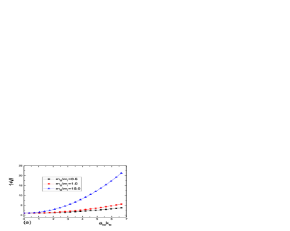
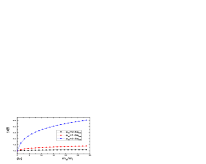
By means of (21), the effective mass of the impurity $m_{I}^{\ast}$

$\displaystyle m_{I}^{\ast}=\frac{m_{I}}{1-\eta}$ (23)

Introducing another parameter $W=\eta/(1-\eta)$ which, in fact, can reflect the effective strength of coupling in contrast to the situation for polaron, the effective mass can be expressed into $m_{I}^{\ast}/m_{I}=1+W$. Integrating the angular variable, $W$ is reduced as

W=8​ρ3​3​π3/2​mBmI​(1+mBmI)2​(kB​aI​B)2(kB​aB​B)1/2​Π(0)π‘Š8𝜌33superscriptπœ‹32subscriptπ‘šπ΅subscriptπ‘šπΌsuperscript1subscriptπ‘šπ΅subscriptπ‘šπΌ2superscriptsubscriptπ‘˜π΅subscriptπ‘ŽπΌπ΅2superscriptsubscriptπ‘˜π΅subscriptπ‘Žπ΅π΅12superscriptΞ 0\displaystyle W=\frac{8\rho}{3\sqrt{3}\pi^{3/2}}\frac{m_{B}}{m_{I}}\left(1+\frac{m_{B}}{m_{I}}\right)^{2}\frac{(k_{B}a_{IB})^{2}}{(k_{B}a_{BB})^{1/2}}\Pi^{(0)} (24)

where

Ξ (0)=∫0βˆžπ‘‘y​y2(y2+2​ρ)1/2​[(y2+2​ρ)1/2+(mB/mI)​y]3superscriptΞ 0superscriptsubscript0differential-d𝑦superscript𝑦2superscriptsuperscript𝑦22𝜌12superscriptdelimited-[]superscriptsuperscript𝑦22𝜌12subscriptπ‘šπ΅subscriptπ‘šπΌπ‘¦3\displaystyle\Pi^{(0)}=\int_{0}^{\infty}dy\frac{y^{2}}{(y^{2}+2\rho)^{1/2}[(y^{2}+2\rho)^{1/2}+(m_{B}/m_{I})y]^{3}}
(25)

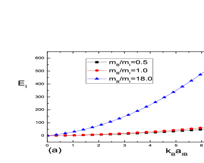
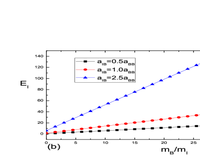
Where in order to scale the expression we define a parameter $k_{B}$ like the Fermi wavevector $n=k_{B}^{3}/(6\pi^{2})$. In addition, we also introduce another notation $\rho=n_{0}/n$ for condensate fraction. From the expression of $W$ and under the approximation (12) which signifies the condensate fraction $\rho$ is independent of $a_{IB}$, we easily find that $W$ is proportional to the square of the $a_{IB}$ for definite the $a_{BB}$ and $m_{B}/m_{I}$. Fig.1(a) apparently respects this kind of behavior. The dependence of $W$ on $m_{B}/m_{I}$ for definite $a_{BB}$ and $a_{IB}$ appears to be indirect due to the dependence of Ξ (0)superscriptΞ 0\Pi^{(0)} on $m_{B}/m_{I}$. Fig.1(b) show the corresponding change of the effective coupling strength as function of $m_{B}/m_{I}$.

Refer to caption
Refer to caption
Figure 1: The behavior of the effective mass $m_{I}^{\ast}/m_{I}=1+W$ as a function of $a_{IB}$ for different mass ratios $m_{B}/m_{I}$ of atom to impurity (a); as a function of mass ratio $m_{B}/m_{I}$ for different boson-impurity scattering length $a_{IB}$ (b). We have chosen $a_{BB}k_{B}=0.87$.

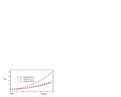
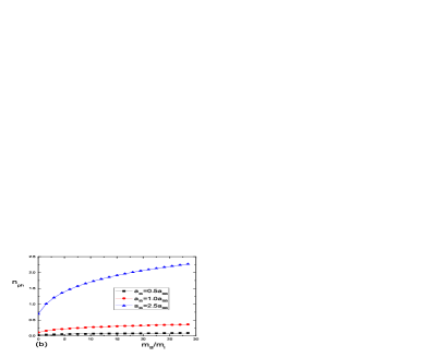
At zero temperature, the number of phonon is zero for purely BEC while there exists some phonon excitations in BEC with an impurity. Below we calculate the phonon number carried by the impurity np​h=βˆ‘k<Ξ¦|bk†​bk|Ξ¦>=βˆ‘k|f​(k)|2subscriptπ‘›π‘β„Žsubscriptπ‘˜quantum-operator-productΞ¦superscriptsubscriptπ‘π‘˜β€ subscriptπ‘π‘˜Ξ¦subscriptπ‘˜superscriptπ‘“π‘˜2n_{ph}=\sum_{k}<\Phi|b_{k}^{{\dagger}}b_{k}|\Phi>=\sum_{k}|f(k)|^{2}

np​h=2​ρ3​π3/2​(kB​aI​B)2(kB​aB​B)1/2​(1+mBmI)2​Π(1)subscriptπ‘›π‘β„Ž2𝜌3superscriptπœ‹32superscriptsubscriptπ‘˜π΅subscriptπ‘ŽπΌπ΅2superscriptsubscriptπ‘˜π΅subscriptπ‘Žπ΅π΅12superscript1subscriptπ‘šπ΅subscriptπ‘šπΌ2superscriptΞ 1\displaystyle n_{ph}=\frac{2\rho}{\sqrt{3}\pi^{3/2}}\frac{(k_{B}a_{IB})^{2}}{(k_{B}a_{BB})^{1/2}}\left(1+\frac{m_{B}}{m_{I}}\right)^{2}\Pi^{(1)} (26)

where

Ξ (1)=∫0βˆžπ‘‘y​y(y2+2​ρ)1/2​1[(y2+2​ρ)1/2+(mB/mI)​y]2βˆ’4​(mB/mI)2​(1βˆ’Ξ·)2​P~2superscriptΞ 1superscriptsubscript0differential-d𝑦𝑦superscriptsuperscript𝑦22𝜌121superscriptdelimited-[]superscriptsuperscript𝑦22𝜌12subscriptπ‘šπ΅subscriptπ‘šπΌπ‘¦24superscriptsubscriptπ‘šπ΅subscriptπ‘šπΌ2superscript1πœ‚2superscript~𝑃2\displaystyle\Pi^{(1)}=\int_{0}^{\infty}dy\frac{y}{(y^{2}+2\rho)^{1/2}}\frac{1}{[(y^{2}+2\rho)^{1/2}+(m_{B}/m_{I})y]^{2}-4(m_{B}/m_{I})^{2}(1-\eta)^{2}\widetilde{P}^{2}} (27)

and $\widetilde{P}=P/(2m_{B}ng)^{1/2}$. When an impurity moves in BEC, the state of this impurity is sensitively dependent on its velocity according to superfluid Landau theory [23]. Landau used simple kinematic arguments to derive an expression for the critical velocity $V_{L}=min[\zeta(k)/k]$ where $\zeta(k)$ is the energy of an elementary excitation with momentum $k$. If the velocity of impurity is larger than $V_{L}$, the impurity will dissipate energy by colliding with BEC, but if not, the impurity will move without dissipation. Such behavior has been predicted theoretically [24] and observed experimentally [10]$\colon$ as the impurity velocity is diminished below Landau critical velocity, there exists a dramatic reduction in the probability of collisions. Recalling that in the process of deriving effective Hamiltonian (10) we have made forward-scattering approximation. Only forward scattering corresponds to no scattering and vanishing collision probability. Thus we think that the reduction of collision probability for low impurity speed smaller than Landau critical velocity can guarantee the validity of forward-scattering approximation. In order to keep this approximation valid, we calculate phonon number $n_{ph}$ at $P=0$. In ionic crystals, the phonon carried by electron is virtual when the energy of moving electron is lower than that of optical phonon which has a finite energy gap. Superficially for BEC system phonon is gapless, no matter how small the velocity of the impurity is, phonon is able to create. But it can also not be created for arbitrary small impurity velocity due to above stated BEC mechanics. So phonon number we calculate is also virtual. Corresponding behavior for phonon number is showed in Fig.2 and is very similar to the behavior of effective mass of impurity. This observation is consistent with our intuition about polaron$\colon$ the more number of the phonon encompassing the impurity, the larger the force dragging the impurity and so the larger the impurity effective mass.

Refer to caption
Refer to caption
Figure 2: The behavior of the phonon number $n_{ph}$ as a function of boson-impurity scattering length $a_{IB}$ for different mass ratios $m_{B}/m_{I}$ of boson to impurity (a); as a function of boson-impurity mass ratio $m_{B}/m_{I}$ for different boson-impurity scattering length $a_{IB}$. We have chosen $a_{BB}k_{B}=0.87$.

Below we calculate energy related to an impurity with zero velocity. The whole energy of system is

$\displaystyle E_{g}(0)$ $\displaystyle=$ $\displaystyle E_{B}+E(0)+\mu n$ (28)
$\displaystyle\approx$ $\displaystyle(gn_{0}^{2}+E_{B})+(\lambda n_{0}+E(0))$

Where we have used (5) and make another approximation $\mu n\approx\mu n_{0}$ which is valid for dilute BEC. The first term on the right hand side in (28) is the energy of pure bosonic system, so the second term gives impurity energy in BEC system. The calculation about energy must be careful. In Hamiltonian (1), we have used the contact interaction to represent the true potential for which its Fourier transformation should fall off at large momentum. This substitution leads to the ultraviolet divergence of the ground state energy, so that a regularization must be forced. In fact, this divergence is not fundamental and can be regularized by way of absorbing more high order scattering contribution into scattering length [25]

$\displaystyle\frac{2\pi a_{IB}\hbar^{2}}{m_{red}}=\lambda-\frac{2m_{red}\lambda^{2}}{\hbar^{2}}\sum_{k}\frac{1}{k^{2}}$ (29)

After taking these measures, the impurity energy $E_{I}$ after scaled by $2\pi\hbar^{2}a_{BB}n/m_{B}$ is

EI=ρ​(1+mBmI)​kB​aI​BkB​aB​B+4​ρ3​π3/2​(1+mBmI)2​(kB​aI​B)2(kB​aB​B)1/2​Π(2)subscript𝐸𝐼𝜌1subscriptπ‘šπ΅subscriptπ‘šπΌsubscriptπ‘˜π΅subscriptπ‘ŽπΌπ΅subscriptπ‘˜π΅subscriptπ‘Žπ΅π΅4𝜌3superscriptπœ‹32superscript1subscriptπ‘šπ΅subscriptπ‘šπΌ2superscriptsubscriptπ‘˜π΅subscriptπ‘ŽπΌπ΅2superscriptsubscriptπ‘˜π΅subscriptπ‘Žπ΅π΅12superscriptΞ 2\displaystyle E_{I}=\rho(1+\frac{m_{B}}{m_{I}})\frac{k_{B}a_{IB}}{k_{B}a_{BB}}+\frac{4\rho}{\sqrt{3}\pi^{3/2}}(1+\frac{m_{B}}{m_{I}})^{2}\frac{(k_{B}a_{IB})^{2}}{(k_{B}a_{BB})^{1/2}}\Pi^{(2)} (30)

where

Ξ (2)=∫0βˆžπ‘‘y​y2​[1[1+(mB/mI)]​y2βˆ’1(y2+2​ρ)1/2​[(mB/mI)​y+(y2+2​ρ)1/2]]superscriptΞ 2superscriptsubscript0differential-d𝑦superscript𝑦2delimited-[]1delimited-[]1subscriptπ‘šπ΅subscriptπ‘šπΌsuperscript𝑦21superscriptsuperscript𝑦22𝜌12delimited-[]subscriptπ‘šπ΅subscriptπ‘šπΌπ‘¦superscriptsuperscript𝑦22𝜌12\displaystyle\Pi^{(2)}=\int_{0}^{\infty}dy\,y^{2}\left[\frac{1}{[1+(m_{B}/m_{I})]y^{2}}-\frac{1}{(y^{2}+2\rho)^{1/2}[(m_{B}/m_{I})y+(y^{2}+2\rho)^{1/2}]}\right] (31)

The corresponding behavior of $E_{I}$ is plotted in Fig.3.

Refer to caption
Refer to caption
Figure 3: The behavior of impurity energy $E_{I}$ as a function of boson-impurity scattering length $a_{IB}$ for different mass ratio $m_{B}/m_{I}$ of boson to impurity (a); as a function of boson-impurity mass ratio $m_{B}/m_{I}$ for different boson-impurity scattering length $a_{IB}$. We have chosen $a_{BB}k_{B}=0.87$.

4 Discussion and Conclusion

At last, we discuss the validity of our approximation (12) in the frame of LLP theory. Following the method calculating $n_{ph}$, (11) equals to

$\displaystyle n=n_{0}+\sum_{k}v_{k}^{2}+\sum_{k}(u_{k}^{2}+v_{k}^{2})\mid f(k)\mid^{2}-2\sum_{k}u_{k}v_{k}f(k)f(-k)$ (32)

After some predigestion and dividing both sides of (32) by $n$

$\displaystyle 1$ $\displaystyle=$ ρ+83​6​π3/2​ρ3/2​(aB​B​kB)3/2+2​ρ3​π3/2​n​(1+mBmI)2​(kB​aI​B)2(kB​aB​B)1/2​Π(3)𝜌836superscriptπœ‹32superscript𝜌32superscriptsubscriptπ‘Žπ΅π΅subscriptπ‘˜π΅322𝜌3superscriptπœ‹32𝑛superscript1subscriptπ‘šπ΅subscriptπ‘šπΌ2superscriptsubscriptπ‘˜π΅subscriptπ‘ŽπΌπ΅2superscriptsubscriptπ‘˜π΅subscriptπ‘Žπ΅π΅12superscriptΞ 3\displaystyle\rho+\frac{8}{3\sqrt{6}\pi^{3/2}}\rho^{3/2}(a_{BB}k_{B})^{3/2}+\frac{2\rho}{\sqrt{3}\pi^{3/2}n}(1+\frac{m_{B}}{m_{I}})^{2}\frac{(k_{B}a_{IB})^{2}}{(k_{B}a_{BB})^{1/2}}\Pi^{(3)} (33)
$\displaystyle-$ ρ22​3​π3/2​n​mImB​(1+mBmI)2​(kB​aI​B)2(kB​aB​B)1/2​1P~​(1βˆ’Ξ·)​Π(4)superscript𝜌223superscriptπœ‹32𝑛subscriptπ‘šπΌsubscriptπ‘šπ΅superscript1subscriptπ‘šπ΅subscriptπ‘šπΌ2superscriptsubscriptπ‘˜π΅subscriptπ‘ŽπΌπ΅2superscriptsubscriptπ‘˜π΅subscriptπ‘Žπ΅π΅121~𝑃1πœ‚superscriptΞ 4\displaystyle\frac{\rho^{2}}{2\sqrt{3}\pi^{3/2}n}\frac{m_{I}}{m_{B}}(1+\frac{m_{B}}{m_{I}})^{2}\frac{(k_{B}a_{IB})^{2}}{(k_{B}a_{BB})^{1/2}}\frac{1}{\widetilde{P}(1-\eta)}\Pi^{(4)}

with

Ξ (3)superscriptΞ 3\displaystyle\Pi^{(3)} $\displaystyle=$ $\displaystyle\int_{0}^{\infty}dy\frac{y^{2}+\rho}{y^{2}+2\rho}\frac{1}{[(y^{2}+2\rho)^{1/2}+(m_{B}/m_{I})y]^{2}-4(m_{B}/m_{I})^{2}\widetilde{P}^{2}(1-\eta)^{2}}$
Ξ (4)superscriptΞ 4\displaystyle\Pi^{(4)} $\displaystyle=$ $\displaystyle\int_{0}^{\infty}dy\frac{1}{(y^{2}+2\rho)[\sqrt{y^{2}+2\rho}+\frac{m_{B}}{m_{I}}y]}\ln\mid\frac{\frac{m_{B}}{m_{I}}y+\sqrt{y^{2}+2\rho}+2\frac{m_{B}}{m_{I}}\widetilde{P}(1-\eta)}{\frac{m_{B}}{m_{I}}y+\sqrt{y^{2}+2\rho}-2\frac{m_{B}}{m_{I}}\widetilde{P}(1-\eta)}\mid$

Equation (32) is the most basic equation from which we can study the effect of single impurity on condensate fraction. For dilute bosonic system, the condensate fraction $\rho$ approaches unit. The density of a typical BEC system in experiments is $10^{13}-10^{15}cm^{-3}$. Although it is small in contrast to typical density of gas, liquid and solid, it remains a large number. From (33) there is a factor $n$ in the denominators of last two terms on the right hand side. If there are lots of impurities, the last two terms would also include a factor proportional to impurity density. So the last two terms are small and negligible in contrast to the first and second terms in the light of the existence of single impurity. In this way the approximation (12) is proven to be valid.

In conclusion, by making Bogoliubov and forward-scattering approximations we have obtained an equivalent Hamiltonian which is similar to the FrΓΆhlich large polaron Hamiltonian and calculate effective mass of impurity, the phonon number carried by the impurity and the impurity energy on a basis of LLP theory. In addition, we also point out the valid range of forward-scattering approximation that the velocity of the impurity must be smaller than Landau critical velocity of BEC system.

Acknowledgement

The work was supported by National Natural Science Foundation of China under Grant No. 10675108.

References

  • [1] M. H. Anderson, J. R. Ensher, M. R. Mattews, C. E. Wieman and E. A. Cornell, Science 269, 198(1995).
  • [2] K. B. Davis, M. -O. Mewex, M. R. Andrews, N. J. V. Druten, D. S. Durfee, D. M. Kurn and W. Ketterle, Phys. Rev. Lett. 75, 3969(1995).
  • [3] C. C. Bradley, C. A. Sackett and R. G. Hulet, Phys. Rev. Lett.78, 985(1997).
  • [4] M. Greiner, O. Mandel, T. Esslinger, T. W. HΓ€nsch and I. Bloch, Nature(London) 415, 39(2002).
  • [5] M. P. A. Fisher, P. B. Weichman, G. Grinstein and D. S. Fisher, Phys. Rev. B40, 546(1989).
  • [6] D. Jaksch, C. Bruder, J. I. Cirac, C. W. Gardiner and P. Zoller, Phys. Rev. Lett. 81, 3108(1998).
  • [7] C. J. Myatt, E. A. Burt, R. W. Ghrist, E. A. Cornell and C. E. Wieman, Phys. Rev. Lett. 78, 586(1997).
  • [8] F. Schreck, G. Ferrari, K. L. Corwin, J. Cubizolles, L. Khaykovich, M.-O. Mewes and C. Salomon, Phys. Rev. A64, 011402(2001).
  • [9] A. G. Truscott, K. E. Strecker, W. I. Mcalexander, G. B. Partridge and R. G. Hulet, Science 291, 2570(2001).
  • [10] A. P. Chikkatur, A. GΓΆrlitz, D. M. Stamper-Kurns, S. Inouye, S. Gupta and W. Ketterle, Phys. Rev. Lett. 85, 483(2000).
  • [11] Z. Hadzibabic, C. A. Stan, K. Dieckmann, S. Gupta, M. W. Zwierlein, A. Gorlitz and W. Ketterle, Phys. Rev. Lett. 88, 160401(2002).
  • [12] G. Roati, F. Riboli, G. Modugno and M. inguscio, Phys. Rev. Lett. 89, 150403(2002).
  • [13] F. M. Cucchietti and E. Timmermans, Phys. Rev. Lett. 96, 210401(2006).
  • [14] R. M. Kalas and D. Blume, Phys. Rev. A73, 043608(2006).
  • [15] K. Sacha and E. Timmermans, Phys. Rev. A73, 063604(2006).
  • [16] L. D. Landau, Phys. Z. Sowjetunion 3, 644(1933).
  • [17] S. I. Pekar, Zh. Eksp. Teor. Fiz. 16, 335(1946).
  • [18] H. FrΓΆhlich, Adv. Phys, 3, 325(1954).
  • [19] H. FrΓΆhlich, Phys. Rev. 79, 845(1950).
  • [20] T. D. Lee, F. E. Low and D. Pines, Phys. Rev. 90, 297(1953).
  • [21] D. van Oosten, P. van der Straten and H. T. C. Stoof, Phys. Rev. A63, 053601(2001).
  • [22] J. Goldstone, Nuovo Cimento, 19, 154(1961).
  • [23] L. D. Landau, J. Phys. (Moscow) 5, 71(1941).
  • [24] E. Timmermans and R. C$\hat{o}$t$\acute{e}$, Phys. Rev. Lett. 80, 3419(1998).
  • [25] A. L. Fetter and J. D. Walecka, Quantum Theory of Many-Particle System (McGraw-Hill, New York, 1971).