Self-consistent microscopic calculations for non-local transport through nanoscale superconductors

Abstract

We implement self-consistent microscopic calculations in order to describe out-of-equilibrium non-local transport in normal metal-superconductor-normal metal hybrid structures in the presence of a magnetic field and for arbitrary interface transparencies. A four terminal setup simulating usual experimental situations is described by means of a tight-binding model. We present results for the self-consistent order parameter and current profiles within the sample. These profiles illustrate a crossover from a quasi-equilibrium to a strong non-equilibrium situation when increasing the interface transparencies and the applied voltages. We analyze in detail the behavior of the non-local conductance in these two different regimes. While in quasi-equilibrium conditions this can be expressed as the difference between elastic cotunneling and crossed Andreev transmission coefficients, in a general situation additional contributions due to the voltage dependence of the self-consistent order parameter have to be taken into account. The present results provide a first step towards a self-consistent theory of non-local transport including non-equilibrium effects and describe qualitatively a recent experiment [Phys. Rev. Lett. 97, 237003 (2006)].

I Introduction

In addition to charge and spin, future electronic devices may also manipulate the non-local correlations allowed by quantum mechanics, known as entanglement. For instance a superconductor may be used as a source of Einstein Podolsky Rosen pairs of electrons Choi ; Martin . Local Andreev reflection Andreev at a normal metal - superconductor (NS) interface is a process by which a spin-up electron incoming from the normal side is reflected as a spin-down hole while a pair is transferred into the superconductor: pairs of electrons penetrate the superconductor for an applied bias smaller than the gap (see Fig. 1a). For an opposite applied voltage, the superconductor S emits correlated pairs of electrons into the normal metal N. Andreev reflection takes place in a coherence volume of size $\xi_{0}$, the characteristic length associated to the superconducting gap $\Delta$. Two separate normal electrodes connected to a superconductor within a distance of order $\xi_{0}$ may thus be coupled by “non-local” or “crossed” Andreev processes ^1,2,4-30 (CAR, see Fig. 1b). On the other hand another type of non-local process may take place. Electrons can also tunnel across the superconductor from one normal electrode to the other. This normal tunneling has been called Falci “elastic cotunneling” (EC) in analogy to similar processes taking place in Coulomb blockaded quantum dots Nazarov .

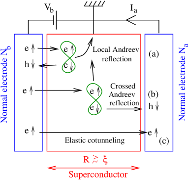
Figure 1: (Color online). Schematic representation of the electrical circuit used in a non-local conductance experiment. The lowest order processes are shown on the figure: local Andreev reflection (a), crossed Andreev reflection (CAR) (b) and elastic cotunneling (EC) (c).

Motivated by the possibility of creation of non-local coherent states by means of CAR processes, several experiments have been performed recentlyBeckmann ; Russo ; Cadden on superconducting structures connected to normal or ferromagnetic metallic electrodes. Depending on the type of S/N interfaces, geometry and range of parameters, different behaviors of the non-local conductance or resistance have been observed.

According to lowest order perturbation theory Falci in the tunnel amplitudes, EC and CAR have the same transmission coefficient, once an average over the Fermi wave-length scale or over disorder is carried out. Since an opposite charge is transmitted by EC and CAR, it is deduced that the non-local conductance vanishes in this limit. A finite non-local signal may be restored by higher order tunneling processesMelin-Feinberg-PRB ; Melin-Duhot-EPJB ; Melin-wl or by Coulomb interactions Levy-Yeyati . Moreover, out-of-equilibrium effects may play an important role on the non-local transport as was suggested in Ref. Golubev, for a superconducting quantum dot and in Ref. Kalenkov, for normal electrodes connected to a three dimensional superconductor.

Experimental data on the other hand are still not well understood. In particular the experiment of Ref. Russo, on a planar NISIN structure (where I stands for an insulating barrier) has provided unexpected experimental evidence for a non-local signal dominated either by EC or by CAR depending on the value of the applied bias. Also importantly, this experiment Russo has shown a suppression of the non-local signal when an external magnetic field, much smaller than the critical one, was applied. Other experiments on NSN hybrid structures provide evidence for charge imbalance effects as the voltage approaches the temperature-dependent gap valueCadden and in a temperature window close to the superconducting critical temperatureBeckmann .

Although non-local transport in SN structures has been addressed theoretically by several works in recent years, none of these provide a full self-consistent model for describing the superconducting order parameter, the current profile and the non-local conductance of the S region, as well as the magnetic field dependence of these quantities.

To bridge this gap, we analyze here a NISIN planar structure using a microscopic model which we solve self-consistently in order to obtain the current profile inside the superconductor in the presence of an applied voltage and magnetic field. To adequately represent a non-local transport measurement setup in the self-consistent calculation it is important to include additional superconducting leads which allow to remove from the sample the injected current (see Fig. 2). This implies a substantial difference with conventional “two terminal” measurements, for which the current is the same on both leads. A two-terminal situation would be recovered by removing the superconducting leads.

An important parameter characterizing an actual experimental situation is the value of the transparency for the barriers connecting the superconductor with the normal electrodes. Although this parameter is difficult to be controlled in experiments the available data correspond to very different ranges as it was pointed out in Ref. beckman2, . Within our model it is possible to study non-local transport for arbitrary interface transparency, applied bias and external magnetic field. This allows us to analyze the crossover from a quasi-equilibrium situation at low barrier transparency to the case of strong non-equilibrium for high transparency and finite voltages. In agreement with previous works Melin-Feinberg-PRB ; Zaikin , we find that increasing barrier transparency leads to a dominance of EC over CAR transmission in the non-local conductance. We also show that an applied magnetic field does not modify the balance between EC and CAR. The value of the EC and CAR transmission coefficients increases upon application of voltage or magnetic field (positive magneto-transmission). For simplicity we do not take into account in the present work the effect of Coulomb interactions, although it has been realized that they can play an important role for the case of low barrier transparencies Levy-Yeyati ; Duhot-Melin-PRB-Hikami . We also restrict our analysis to the ballistic case at zero temperature.

In addition to providing insight into the gap and current profiles in the superconducting region, our work demonstrates that a description of non-local transport in terms of linear relations involving the EC and CAR transmission coefficients only makes sense in a quasi-equilibrium situation when either the transparency of the S/N interfaces or the bias voltage is low. If the superconductor is driven far from the equilibrium situation this description breaks down, and the resulting non-local conductance and resistance deviate considerably from their values in equilibrium. This case corresponds to the experimental situation of Ref. Cadden, where the non-local resistance was measured for currents close to the critical one. Within our model we are able to obtain the observed change of sign of the non-local resistance as a function of the injected currentCadden . In particular we demonstrate that this change of sign is related to the suppression of the local conductance and not due to the dominance of CAR over EC processes.

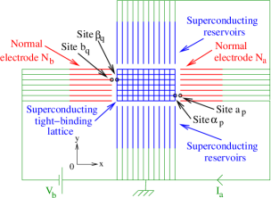
Figure 2: (Color online). Schematic representation of the tight-binding model used in our simulations and of the electrical circuit (green lines). The self-consistent gap is evaluated on a square lattice with $M=R_{y}/a_{0}$ transverse channels and a length $R_{x}=Na_{0}$, with $a_{0}$ the lattice spacing. Normal electrodes N_b (N_a) are connected to the square lattice at left (right). Superconducting reservoirs (with zero superconducting phase) are connected on top and bottom. The normal and superconducting electrodes are modeled by a collection of one dimensional channels.

The article is organized as follows. In the next Sec. II we describe the model for a multiterminal NSN structure based on a tight-binding Hamiltonian with a local pairing which will be determined self-consistently. We also give details on how the electronic and transport properties of this model are obtained with the help of non-equilibrium Green functions. In Sec. III we present results for the behavior of the complex order parameter and the current profiles in the presence of an applied magnetic field, applied voltage and different values of the barrier transparency. We also analyze the behavior of the non-local conductance for both the quasi-equilibrium and non-equilibrium regimes. Concluding remarks are provided in Sec. IV.

II Model for a multiterminal NSN structure

We consider a superconducting region whose thickness is much smaller than the coherence and the London penetration lengths. This region is connected to four electron reservoirs as shown in Fig. 2.

We describe the central superconducting region by means of a tight-binding model on a square lattice:

$${\cal H}_{BCS} = -\sum_{\langle k,l\rangle,\sigma}\left(t_{kl}c_{l,\sigma}^{+}c_{k,\sigma}+t_{l,k}c_{k,\sigma}^{+}c_{l,\sigma}\right)$$ (1)

$$+ \sum_{k}\Delta_{k}\left(c_{k,\uparrow}^{+}c_{k,\downarrow}+c_{k,\downarrow}^{+}c_{k,\uparrow}\right)\;.$$

The variable $\Delta_{k}$ in Eq. (1) is the superconducting order parameter at site $k$ and a summation over pairs of neighboring sites $\langle k,l\rangle$ is carried out in the kinetic term. In order to take into account the effect of a magnetic field ${\bf B}={\bf rotA}$ one should introduce a phase in the hopping elements

$$t_{kl}=t\exp{\left(\frac{2i\pi}{\phi_{0}}\int_{{\bf r}_{k}}^{{\bf r}_{l}}{\bf A}({\bf r}).{\bf dr}\right)},$$ (2)

where ${\bf A}({\bf r})$ is the vector potential, and $\phi_{0}=h/e$ is the flux quantum. In the following the magnetic field will be measured in terms of $\phi/\phi_{0}$, i.e. the total flux through the central region in units of $\phi_{0}$. Disorder could be introduced in the form of an on-site random potential on each tight-binding site. We use the notations $R_{x}=Na_{0}$ and $R_{y}=Ma_{0}$ for the dimensions of the lattice, where $a_{0}$ denotes the lattice spacing.

The central superconducting region is connected at the left to the normal electrode N_b and at the right to the normal electrode N_a. In order to model a real experimental situation for non-local transport we connect the top and bottom of the central region to superconducting reservoirs (see Fig. 2) by highly transparent interfaces. Thus, a current injected through the left interface can flow into these reservoirs. The leads, both the normal and superconducting, are described by independent one dimensional wires connected to each of the lateral sites of the central superconducting region. By varying the hopping terms $t_{a}$ and $t_{b}$ connecting the central region to the normal leads one can control the interface transparency $T_{N}$ between $0$ and $1$. The hopping parameter in the rest of the system is assumed to have the same value $t$.

Calculational Methods

The transport properties of this model can be conveniently expressed in terms of the retarded $G^{r}$, advanced $G^{a}$ and Keldysh $G^{+-}$ Green functions, which are matrices in the Nambu space and depend on two site labels $k,l$.

The Nambu representation of the central region Hamiltonian takes the form

$$\hat{h}_{kl}=\left(\begin{array}[]{cc}0&\Delta_{k}\\ \Delta_{k}^{*}&0\end{array}\right)\;\delta_{kl}+\left(\begin{array}[]{cc}t_{kl}&0\\ 0&-t_{kl}^{*}\end{array}\right)\;(1-\delta_{kl}),$$ (3)

where $t_{kl}$ is restricted to first neighbors and was defined in Eq. (2).

The advanced and retarded Green functions are obtained from a recursive algorithm. To this end we divide the central square lattice into layers along the $y$ direction which we label by an index $n$ ($1\leq n\leq N$). We denote by $\hat{\bf G}^{a}_{n,n}$ the Nambu advanced Green function projected on the sites corresponding to the $n$ layer. This is obtained as

$$\hat{\textbf{G}}^{a}_{n,n} = \left[\omega-\hat{\bf\Sigma}_{n}-\hat{\textbf{T}}_{n,n-1}\hat{\textbf{\cal g}}^{L}_{n-1}\hat{\textbf{T}}_{n-1,n}\right.$$

$$\left.-\hat{\textbf{T}}_{n,n+1}\hat{\textbf{\cal g}}^{R}_{n+1}\hat{\textbf{T}}_{n+1,n}\right]^{-1}\;,$$

where the recursions take the form

$$\hat{\textbf{\cal g}}^{L}_{n} = \left[\omega-\hat{\bf\Sigma}_{n}-\hat{\textbf{T}}_{n,n-1}\hat{\textbf{\cal g}}^{L}_{n-1}\hat{\textbf{T}}_{n-1,n}\right]^{-1}$$ (5)

$$\hat{\textbf{\cal g}}^{R}_{n} = \left[\omega-\hat{\bf\Sigma}_{n}-\hat{\textbf{T}}_{n,n+1}\hat{\textbf{\cal g}}^{R}_{n+1}\hat{\textbf{T}}_{n+1,n}\right]^{-1},$$ (6)

with the boundary conditions $\hat{\textbf{\cal g}}^{L}_{0}=\hat{\textbf{\cal g}}^{R}_{N+1}=(i/t)\hat{\bf I}$, corresponding to the uncoupled normal wires in the wide band approximation. In the recursive equations $(\hat{\bf\Sigma}_{n})_{kl}=\hat{h}_{kl}+t\hat{\sigma}_{z}\hat{g}_{S}\hat{\sigma}_{z}\delta_{kl}(\delta_{k1}+\delta_{kM})$ with $\hat{g}_{S}=(-\omega\hat{I}+\Delta_{0}\hat{\sigma}_{x})/\sqrt{\Delta_{0}^{2}-\omega^{2}}$, is the local self-energy on the $n$ layer and $\hat{\bf T}_{n,n\pm 1}$ contains the hopping elements connecting neighboring layers. In the last expression we have introduced the usual Pauli matrices in Nambu space $\hat{\sigma}_{z}$ and $\hat{\sigma}_{x}$. The dependence on energy $\omega$ is implicit in the Green functions in Eqs. (II)-(6). The Green function connecting two arbitrary layers $n$ and $m$ can then be obtained from the relations $\hat{\bf G}^{a}_{n,m}=\hat{\bf G}^{a}_{n,m-1}\hat{\bf T}_{m-1,m}\hat{\bf g}^{R}_{m}$ or $\hat{\bf G}^{a}_{n,m}=\hat{\bf G}^{a}_{n,m+1}\hat{\bf T}_{m+1,m}\hat{\bf g}^{L}_{m}$. In the absence of voltage applied on electrode N_b, the Keldysh Green function of the superconductor takes the equilibrium form

$$\hat{\bf G}^{+-,eq}_{n,n}(\omega)=n(\omega)\left(\hat{\bf G}^{a}_{n,n}(\omega)-\hat{\bf G}^{r}_{n,n}(\omega)\right),$$ (7)

where $n(\omega)$ is the Fermi distribution function with zero chemical potential. When a voltage $V_{b}$ is applied on electrode N_b the Keldysh Green function of row $n$ is given by

$$\hat{\bf G}^{+-}_{n,n}(\omega) = \hat{\bf G}^{+-,eq}_{n,n}(\omega)$$

$$+ \hat{\bf G}^{R}_{n,1}(\omega)\hat{\bf T}_{1,0}\delta\hat{\bf g}^{+-}_{0}(\omega)\hat{\bf T}_{0,1}\hat{\bf G}^{A}_{1,n}(\omega),$$

where

$$\delta\hat{\bf g}^{+-}_{0}(\omega)=\frac{2i}{t}\left(\begin{array}[]{cc}\delta n_{e}&0\\ 0&\delta n_{h}\end{array}\right)\hat{\bf I}\;,$$ (9)

with (assuming zero temperature)

$$\delta n_{e}(\omega) = \theta(-\omega+eV_{b})-\theta(-\omega)$$ (10)

$$\delta n_{h}(\omega) = \theta(-\omega-eV_{b})-\theta(-\omega).$$ (11)

The pairing amplitude in the superconductor is set by the anomalous component of the Keldysh Green function given by Eq. (II). Self-consistency equations at each site $k$ take the form

$$\Delta_{k}=\lambda\int\frac{d\omega}{2i\pi}\left[\hat{G}^{+-}_{kk}(\omega)\right]_{12}\;,$$ (12)

where $\lambda$ is the strength of the attractive electron-electron interaction. This is chosen in order to obtain the same gap parameter $\Delta_{0}$ as in the upper and lower superconducting leads in equilibrium conditions. Eq. (12) is iterated until self-consistency is achieved. The self-consistent gap, the current flow in the superconductor and the non-local conductance are then evaluated.

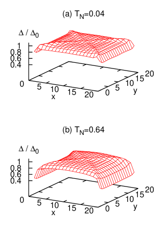
Figure 3: (Color online). Self-consistent gap profile at zero voltage for a system size $R_{x}/a_{0}=R_{y}/a_{0}=20$ and two different values of the normal transparency.

The current flowing from site $k$ to site $l$ is given by

$$I_{kl}=\frac{2e}{h}\int d\omega\left[\hat{t}_{kl}\hat{G}^{+-}_{lk}(\omega)-\hat{t}_{lk}\hat{G}^{+-}_{kl}(\omega)\right]_{11}.$$ (13)

A stringent test of self-consistency is provided by current conservation at each site of the central region because current is conserved only once self-consistency is verifiedyeyati95 .

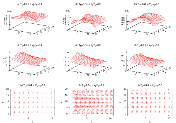
Figure 4: (Color online). Order parameter and current profiles for a sample size $R_{x}/a_{0}=12$, $R_{y}/a_{0}=20$ under an applied voltage $V_{b}$. The upper panels show the profiles of the self-consistent gap. The gap is normalized to its valued $\Delta_{0}$ in the superconducting reservoirs. The voltage is indicated by an arrow on the vertical axis. The middle panels show the phase profile and the lower ones the corresponding current maps. The size of the arrows in the three lower panels is proportional to the value of the local current, with the same scaling factor for the three panels. The values of the parameters $T_{N}$ and $V_{b}$ are indicated on top of each panel.

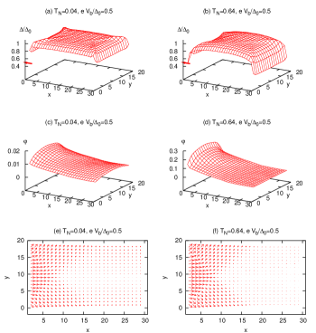
Figure 5: (Color online). Same as Fig. 4 for sample dimensions $R_{x}/a_{0}=30$ and $R_{y}/a_{0}=20$. The scaling factor between current and size of arrow is not the same as in Figs. 4g, h and i, and it is different for panels e and f.

The non-local conductance can be computed as ${\cal G}_{a,b}(V_{a},V_{b})=\partial I_{a}/\partial V_{b}(V_{a},V_{b})$, where $I_{a}(V_{a},V_{b})=\sum_{p}I_{a_{p}\alpha_{p}}(V_{a},V_{b})$ is the total current flowing to electrode N_a in response to voltages $V_{a}$ and $V_{b}$ on electrodes a and b. We use here $V_{a}=0$, as in available experiments Russo ; Cadden ; Beckmann . The notation $a_{p}$ ($b_{q}$) is used for the site at the right (left) interface formed by the superconductor and the normal channel $p$ ($q$), while $\alpha_{p}$ ($\beta_{q}$) are used for the counterpart in the superconductor (see Fig. 2). In quasi-equilibrium conditions, i.e. when the variation of the self-consistent order parameter with $V_{b}$ is negligible, the non-local conductance can be written as Melin-Feinberg-PRB

$${\cal G}_{a,b}(eV_{b})=\frac{e^{2}}{h}\left(T_{CAR}(eV_{b})-T_{EC}(eV_{b})\right),$$ (14)

where the EC and CAR transmission coefficients in the present model are given by

$$T_{EC}(eV_{b}) = 2t_{a}^{2}t_{b}^{2}/t^{2}\sum_{p,q}\left(\left[\hat{G}_{\alpha_{p},\beta_{q}}^{a}(eV_{b})\right]_{11}\left[\hat{G}_{\beta_{q},\alpha_{p}}^{r}(eV_{b})\right]_{11}+\left[\hat{G}_{\alpha_{p},\beta_{q}}^{a}(eV_{b})\right]_{22}\left[\hat{G}_{\beta_{q},\alpha_{p}}^{r}(eV_{b})\right]_{22}\right)$$

$$T_{CAR}(eV_{b}) = 2t_{a}^{2}t_{b}^{2}/t^{2}\sum_{p,q}\left(\left[\hat{G}_{\alpha_{p},\beta_{q}}^{a}(eV_{b})\right]_{12}\left[\hat{G}_{\beta_{q},\alpha_{p}}^{r}(eV_{b})\right]_{21}+\left[\hat{G}_{\alpha_{p},\beta_{q}}^{a}(eV_{b})\right]_{21}\left[\hat{G}_{\beta_{q},\alpha_{p}}^{r}(eV_{b})\right]_{12}\right).$$

The sum over $p$ and $q$ in Eqs. (LABEL:eq:TEC) and (LABEL:eq:TCAR) corresponds to a sum over all one dimensional transverse channels in the normal electrodes. As mentioned above, the parameters $t_{a}$ and $t_{b}$ are the hopping amplitudes connecting electrodes N_a and N_b to the superconductor.

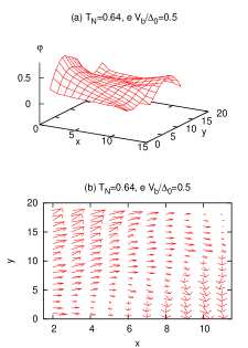
Figure 6: (Color online). (a) Surface map of the self-consistent phase under magnetic field, for sample dimensions $R_{x}/a_{0}=12$ and $R_{y}/a_{0}=20$. The corresponding current map is shown on (b). The flux is $\phi/\phi_{0}=1$. The scaling factor between current and size of arrow is the same as in Figs. 4g, h and i.

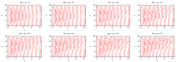
Figure 7: (Color online). Current map for increasing values of the magnetic flux $\phi/\phi_{0}$ and for $T_{N}=0.64$, $R_{x}/a_{0}=12$ and $R_{y}/a_{0}=20$. The applied voltage $V_{b}$ is set to $0.9\Delta_{0}$. An arrow with the same length corresponds to the same current for all panels. The scaling factor between current and size of arrow is the same as in Figs. 4g, h and i.

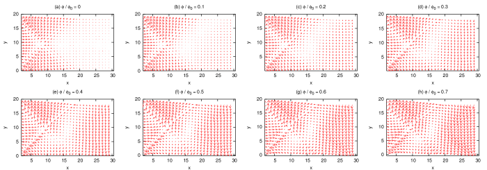
Figure 8: (Color online). Same as in Fig. 7 for $T_{N}=0.64$, $eV_{b}=0.9\Delta_{0}$, $R_{x}/a_{0}=30$ and $R_{y}/a_{0}=20$.

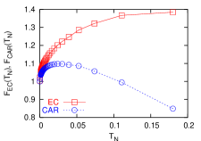
Figure 9: (Color online). Variation of the quantities $F_{EC}(T_{N})$ and $F_{CAR}(T_{N})$ defined in text, as a function of the normal transparency $T_{N}$. A predominance of EC over CAR is obtained for high values of interface transparencies. The chosen system dimensions are $R_{x}=28a_{0}$ and $R_{y}=20a_{0}$.

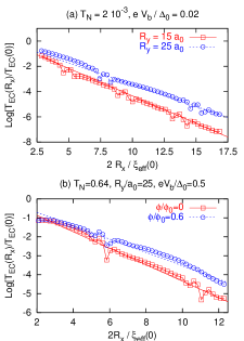
Figure 10: (Color online). Dependence of the EC transmission coefficient on the length $R_{x}=Na_{0}$ of the superconductor. Panel (a) corresponds to low transparency and two different values of the transverse dimension $R_{y}=15$ and $25a_{0}$. The sample dimension $R_{x}$ on panel (a) is normalized to the value $\xi_{eff}(0)$ of the coherence length for $R_{y}=15a_{0}$. Panel (b) corresponds to high transparency and two different values of the magnetic flux. The sample dimension on panel (b) is normalized to the value $\xi_{eff}(0)$ of the coherence length for $\phi/\phi_{0}=0$. Out-of-equilibrium effects are negligible for both panels (see insets of Fig. 12).

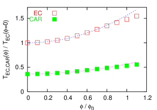
Figure 11: (Color online). Dependence of the transmission coefficients $T_{EC}(\phi)/T_{EC}(\phi=0)$, and $T_{CAR}(\phi)/T_{EC}(\phi=0)$ on the magnetic flux $\phi/\phi_{0}$. We have chosen $T_{N}=0.64$, $R_{x}/a_{0}=20$ and $R_{y}/a_{0}=14$. The broken and dotted lines indicate the quadratic fit of Eq.(19).

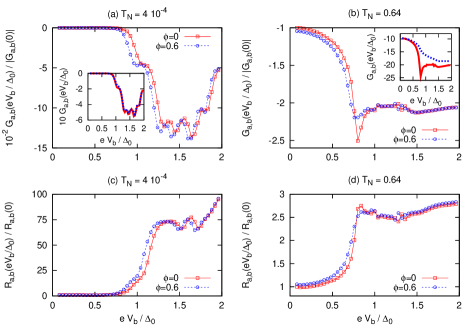
Figure 12: (Color online). Voltage dependence of the non-local conductance (upper panels), and of non-local resistance (lower panels), normalized to their value at zero bias in zero applied magnetic field. The values of $T_{N}$ and $\phi$ are indicated on each panel. The insets of the upper panels illustrate the comparison between the full calculation ${\cal G}_{a,b}=\partial I_{a}/\partial V_{b}$ (solid line) and the expression approximation ${\cal G}_{a,b}=e^{2}/h(T_{CAR}-T_{EC})$ with the transmission coefficients defined by Eqs. (LABEL:eq:TEC) and (LABEL:eq:TCAR) (dashed line). The non local conductance ${\cal G}_{a,b}$ in the insets is given in units of $e^{2}/h$.

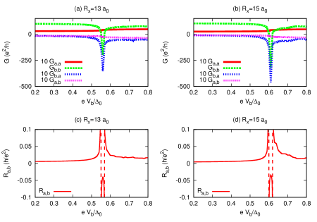
Figure 13: (Color online). Voltage dependence of the local and non-local conductances (upper panels) and of the non-local resistance (lower panels) for an asymmetric junction with $T_{N}=1$ at the $b$ interface and $T_{N}=0.1$ at the $a$ side, for $R_{y}=40a_{0}$ and two values of $R_{x}$: $13a_{0}$ [panels (a) and (b)] and $15a_{0}$ [panels (c) and (d)].

III Results

III.1 Self-consistent gap, phase and current profiles

As a first step it is instructive to analyze the behavior of the complex order parameter which is obtained from the self-consistency Eq. (12). In order to be able to accurately describe the spatial variations with a reasonable computational cost we fix $\Delta_{0}/t=0.1$, which roughly corresponds to a coherence length $\xi_{0}\simeq 7a_{0}$. The system sizes that we consider in this work correspond typically to $R_{x},R_{y}\sim 12-30\,a_{0}$ but in some cases we use $R_{x}$ up to $60a_{0}$ and $R_{y}$ up to $40a_{0}$.

The profile of the self-consistent order parameter amplitude (gap) at zero voltage and zero magnetic field is shown on Fig. 3 for a low ($T_{N}=0.04$) and a high ($T_{N}=0.64$) values of the interface transparencies. As can be observed the gap is reduced at the contacts with the normal leads due to the inverse proximity effect. This gap suppression becomes stronger as the interface transparency increases. There is also a slight suppression on the contacts with the upper and lower superconducting reservoirs which appears due to its deviation from an ideal interface. On the other hand, in equilibrium and for sufficiently large system size the gap in the middle of the central superconducting region is close to its value in the reservoirs. One can also notice that the gap profiles exhibit small ripples along certain directions, which in the case of a square region ($R_{x}=R_{y}$) correspond to the diagonal lines. These ripples reflect the ballistic character of our model which leads to constructive interference along semi-classical trajectories (for a discussion see Appendix).

An applied voltage on the left electrode N_b leads to several modifications in the order parameter profiles. This is illustrated in Figs. 4 and 5 for system sizes $R_{x}=12a_{0}$ and $R_{x}=30a_{0}$. First, there is a reduction in the average gap value due to depairing effects. This reduction is more pronounced near the contact where the current is injected. It is interesting to note that for the short system and high transparency [panel (b) in Fig. 4] the average gap becomes smaller than the applied voltage for $V_{b}/\Delta_{0}=0.9$. In contrast for samples with $R_{x}$ sufficiently large compared to the coherence length, the overall gap profile is less sensitive to the applied voltage even for high transparency [panel (b) in Fig. 5].

Secondly, the application of a finite voltage $V_{b}$ leads to a smooth drop of the phase of the order parameter along the $x$ direction [panels (d)-(f) in Fig. 4 and (c)-(d) in Fig. 5]. As can be observed this is accompanied by a phase gradient in the $y$ direction which changes sign at the midpoint $y=R_{y}/2$.

The properties of the self-consistent solution can be understood more physically by analyzing the current profiles. These are shown in the lower panels of Figs. 4 and 5. As a general remark, the profiles illustrate how the injected current from the left electrode gradually leaks to the upper and lower superconducting electrodes. As expected, the amount of current reaching the right normal lead is controlled by the barrier transparency, the applied voltage and the system size. For sufficiently large system size one can clearly appreciate an exponential suppression of the injected current on the $\xi_{0}$ scale [panels (e) and (f) in Fig. 5]. In addition the current profiles in the case of the larger system exhibit some structure along the lines $y=x$ and $y=R_{y}-x$ which can be associated with the already mentioned ripples appearing in the gap profiles.

In the presence of applied voltage and magnetic field the phase profile becomes more complex with a modulation both in the $x$ and $y$ directions. As shown in Fig. 6 this is associated with the appearance of currents along the $y$ direction which tend to screen the applied field. These currents are essentially superimposed to the profile arising from the injected current through the left electrode. On the other hand, for this range of parameters the effect of the magnetic field on the amplitude of the order parameter corresponds to a uniform reduction (not shown here).

The superposition of injected and screening currents can be clearly observed in the evolution of the current profiles for increasing values of the magnetic field, shown in Figs. 7 and 8 for the cases $R_{x}=12a_{0}$ and $R_{x}=30a_{0}$ respectively. These plots correspond to the case of high transparency ($T_{N}=0.64$) and high voltage ($V_{b}=0.9\Delta_{0}$) for which the injected and screening currents have a similar size when $\phi/\phi_{0}\simeq 1$. For a given total flux $\phi$ the screening currents are, however, smaller for the case of the shorter system due to the larger gap suppression induced by size effects and by the applied voltage.

III.2 Low bias non-local conductance

In this subsection we analyze the non-local transport properties in the regime $eV_{b}\ll\Delta_{0}$. As discussed in the section on calculational methods the non-local conductance in quasi-equilibrium conditions can be decomposed into EC and CAR contributions, given by Eqs. (LABEL:eq:TEC) and (LABEL:eq:TCAR). These two contributions cannot be disentangled in experiments, but theoretically it is convenient to analyze them in a separate way, especially in the case of low transparency tunnel barriers where the two contributions nearly cancel in the non-local conductanceFalci .

The variation of the low bias EC and CAR transmission coefficients with barrier transparency $T_{N}$ is shown on Fig. 9. We find it convenient to represent in this figure the quantities $F_{EC}(T_{N})$ and $F_{CAR}(T_{N})$ defined as

$$F_{EC}(T_{N}) = \frac{(T_{N})^{-2}T_{EC}(T_{N})}{\lim_{T_{N}\rightarrow 0}(T_{N})^{-2}T_{EC}(T_{N})}$$ (17)

$$F_{CAR}(T_{N}) = \frac{(T_{N})^{-2}T_{CAR}(T_{N})}{\lim_{T_{N}\rightarrow 0}(T_{N})^{-2}T_{EC}(T_{N})}.$$ (18)

This normalization allows to analyze the variation of $T_{EC}$ and $T_{CAR}$ beyond the dominant $\sim T_{N}^{2}$ dependence which is common to both coefficients. As can be observed, transmission of electrons dominates over crossed Andreev processes for highly transparent interfaces while they become almost equal in the $T_{N}\rightarrow 0$ limit. This is an effect previously discussed in literatureFalci ; Melin-Feinberg-PRB which is not modified significantly in our self-consistent calculation.

It is also interesting to analyze the dependence of the EC and CAR coefficients on the superconductor length $R_{x}$. This is illustrated in Fig. 10. We choose to represent in this figure only $T_{EC}$ as $T_{CAR}$ exhibits the same distance behavior. We find that except for tiny fluctuations at certain values of $R_{x}$ the normalized transmission coefficients follow an exponential decay with sample dimensions of the type $T(R_{x})\sim\exp{\left(-2R_{x}/\xi_{eff}\right)}$, where $\xi_{eff}$ is an effective coherence length which is sensitive to the applied voltage and magnetic field. As shown in panel (a) of Fig. 10, the effective coherence length is also sensitive to the transverse dimension $R_{y}$, increasing slightly as $R_{y}$ increases. From Fig. 10a we can estimate the values of $\xi_{eff}$. The coherence length for $R_{y}=15a_{0}$ is $\xi_{eff}\sim 7a_{0}$, while for $R_{y}=25a_{0}$ is $\xi_{eff}\sim 8.8a_{0}$. The increase of $\xi_{eff}$ by increasing $R_{y}$ is due to the enhancement of the inverse proximity effect which reduces the average gap in the S region.

On the other hand, panel (b) on Fig. 10 illustrates the increase of $\xi_{eff}$ when a magnetic field is applied. The coherence length for $\phi/\phi_{0}=0.6$ is $20\,\%$ larger than for $\phi/\phi_{0}=0$, which again can be associated to the reduction of the average gap, now due to the depairing effect of the applied magnetic field.

As can be more clearly observed for low transparency, the transmission coefficients show small fluctuations around $R_{x}\simeq pR_{y}$, with $p$ being an integer. This is another feature associated with the ballistic character of our model as it is discussed in the Appendix.

Finally, Fig. 11 shows the flux dependence of the EC and CAR transmission coefficients. We find that this dependence can be fitted as

$$T_{EC,CAR}(\phi) = T_{EC,CAR}(\phi=0)\left[1+\left(\frac{\phi}{\phi_{*}}\right)^{2}\right],$$ (19)

where $\phi_{*}/\phi_{0}$ is roughly of order unity. For instance, the same value $\phi_{*}/\phi_{0}=1.35\pm 0.05$ for the EC and CAR transmission coefficient is obtained within error-bars for the data on Fig. 11.

III.3 Non-local conductance at arbitrary bias

At arbitrarily large bias the non-local conductance cannot be obtained from Eq. (14) with the transmission coefficients defined by Eqs. (LABEL:eq:TEC) and (LABEL:eq:TCAR) as it contains contributions due to the voltage dependence of the self-consistent order parameter in the S region. More generally it can be computed directly as $\partial I_{a}/\partial V_{b}$.

The upper panels of Fig. 12 illustrate the behavior of ${\cal G}_{a,b}$ at arbitrary bias for a system size $(R_{x},R_{y})=(14a_{0},20a_{0})$ and two different values of the normal transparency $T_{N}$. For small $T_{N}$ the non-local conductance exhibits a abrupt jump for $eV_{b}\sim\Delta_{0}$. In this limit ${\cal G}_{a,b}$ is well described by Eq. (14) [see inset in panel (a)] which is a consequence of having a quasi-equilibrium situation in the whole voltage range. This is also reflected in the magnetic field dependence which remains similar to the one found at low bias. In contrast, for high transparency non-equilibrium effects manifest in several features of the non-local conductance. For instance one can clearly notice that the jump associated to the gap appears at lower voltage bias (Fig.12 b). Also, as shown in the inset, the actual value of ${\cal G}_{a,b}$ deviates from the one calculated from Eq. (14). Finally, it is found that the magnetic field at voltages $\sim\Delta_{0}$ reduces the non-local conductance, i.e. it has the opposite effect to the one found at low bias.

In order to make contact with existing experiments it is also interesting to analyze the behavior of the non-local resistance, defined as

$${\cal R}_{a,b}=-{\cal G}_{a,b}/[{\cal G}_{a,a}{\cal G}_{b,b}-{\cal G}_{a,b}{\cal G}_{b,a}]$$ (20)

where ${\cal G}_{a,a}$ and ${\cal G}_{b,b}$ denote the local conductances at each interface and ${\cal G}_{a,b}$ and ${\cal G}_{b,a}$ are the non local conductances. The later take approximately the same value under quasi-equilibrium conditions, but they are in general different due to the voltage dependence of the superconducting order parameter. Eq. (20) is valid provided that the induced voltage $V_{a}$ is very small and under the assumption that the current voltage relations can be linearized around the voltage $V_{b}$ under consideration. The corresponding results are shown in the lower panels of Fig. 12. While ${\cal R}_{a,b}$ is almost constant in the region of small voltages it exhibits a high increase around the self-consistent gap.

Even stronger non-equilibrium effects are found when increasing the transverse dimension $R_{y}$ and for higher values of the normal transparency $T_{N}$ at the $b$ side while maintaining at $a$ at low values. In that case most of the injected current flows into the superconducting electrode and one can obtain an abrupt jump in ${\cal R}_{a,b}$ from positive to negative for $V_{b}$ of the order of the self-consistent gap note . The origin of this change of sign can be understood from the results in Fig. 13 where the local and non-local conductances are plotted for different values of $R_{x}$ (upper panels). As can be observed, the local conductances exhibit a decrease for voltages approaching the self-consistent gap. This decrease can even lead to a negative local differential conductance which arises due to the fact that the injected current can become larger than the maximum supercurrent that can leak into the superconducting electrode. A similar effect was described in Ref. zaitsev, . This effect is reduced by increasing the length $R_{x}$.

As a consequence of the suppression of the local conductances there exists a voltage window where one can have ${\cal G}_{a,b}{\cal G}_{b,a}>{\cal G}_{a,a}{\cal G}_{b,b}$ which, according to Eq (20), leads to a change of sign in the non-local resistance. It is worth emphasizing that this change of sign is not related to a change of sign of ${\cal G}_{a,b}$ and therefore not associated to a possible dominance of CAR over EC processes. These results are in qualitative agreement with the experimental data of Ref. Cadden, .

We plot in the lower panels of Fig. 13 the variation of ${\cal R}_{a,b}$ as a function of $V_{b}$. One can observe that the abrupt change of sign in ${\cal R}_{a,b}$ reduces its amplitude and shifts towards higher voltages as $R_{x}$ increases. The shift corresponds to the increase of the critical current of the central region which grows linearly with $R_{x}$, an effect which is not present in the data of Ref. Cadden, as it corresponds to a somewhat different geometry. Moreover, while our calculations have been performed in the voltage biased case, the experiments of Ref. Cadden, correspond to a current biased situation. Thus, the regions of negative differential conductance could not be explored. However, the regions with negative ${\cal R}_{a,b}$ shown in the lower panels of Fig. 13 would be observable, since the sign change of ${\cal R}_{a,b}$ is related to the condition ${\cal G}_{a,a}{\cal G}_{b,b}<{\cal G}_{a,b}{\cal G}_{b,a}$ rather than to the change of sign of ${\cal G}_{b,b}$. In fact, we have checked that the change of sign of ${\cal R}_{a,b}$ takes place outside the regions with negative ${\cal G}_{b,b}$.

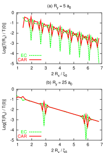
Figure 14: (Color online). Dependence of the normalized EC and CAR transmission coefficients $T(R_{x})/T(0)$ on $2R_{x}/\xi_{0}$, where $R_{x}$ is the dimension of the superconductor along $x$ axis, and $\xi_{0}$ is the bulk coherence length. The applied voltage is small compared to the gap ($eV_{b}/\Delta_{0}=0.02$). The coherence length is larger than for the corresponding parameters that in the presence of superconducting leads. Panel (a) corresponds to $R_{y}=5\,a_{0}$ and panel (b) to $R_{y}=25\,a_{0}$. The symbols correspond to EC and the bold red lines to CAR.

IV Conclusions

We have presented self-consistent model calculations for describing a typical experimental setup to measure non-local transport in nanoscale superconductors connected to normal electrodes. An important ingredient in these calculations is the inclusion of the superconducting leads which drain the current injected into the nanoscale region.

We have found that this system exhibits a rich variety of behaviors controlled by several parameters. One can distinguish two limiting cases: the quasi-equilibrium regime in which the superconducting order parameter depends only weakly on the applied voltage and the strong non-equilibrium case where this dependence cannot be neglected. In these two regimes the non-local conductance exhibits a quite different behavior. In quasi-equilibrium conditions ${\cal G}_{a,b}$ can be expressed as the difference between $T_{CAR}$ and $T_{EC}$. We have shown that $T_{EC}$ becomes larger than $T_{CAR}$ for increasing transparency, and that both decay exponentially with the system size $R_{x}$. Moreover we have shown that both coefficients increase under an applied magnetic field.

In the case of strong non-equilibrium a simple expression of ${\cal G}_{a,b}$ as the difference between $T_{CAR}$ and $T_{EC}$ is no longer possible. The voltage dependence of the self-consistent order parameter introduces an additional contribution to the non-local conductance. We have also found that even the local conductance can be strongly modified by non-equilibrium effects. The effects on these two quantities lead to a non-local resistance which may exhibit a strongly non-monotonous behavior as a function of the injected current including a sign change for sufficiently large transparency.

As a final remark we would like to comment the possible connection between the present model calculations and the existing experiments on non-local transport. As mentioned in the introduction, basically three different experiments have been performed so far. They correspond to different geometries and to different materials. The size of the junctions transparency can also change enormously from one experiment to the other. It is thus not possible to infer general conclusions from these results. In the case of the experiment of Ref. Russo, the authors claim to have junctions with a extremely small transparency $\sim 10^{-5}$ which would warrant the quasi-equilibrium conditions in the subgap voltage range. The results of the present work, corresponding to a non-interacting theory, would not be able to describe that experiment. In particular our results predict an increase of the non-local conductance with magnetic field in contradiction with the experimental observations. As stated in a previous work by some of the authors Levy-Yeyati , interactions mediated by the electromagnetic modes may play an important role in that experimental situation. It was also conjectured Duhot-Melin-PRB-Hikami that disorder may play a role when associated to phase fluctuations.

On the other hand, the experimental results of Ref. Cadden, clearly correspond to the strong non-equilibrium situation described in the present work. Even when our model geometry does not fully correspond the their experimental setup the behavior of the non-local resistance as a function of the injected current shown in Fig.13 is very similar to the one found in this experiment. A closer comparison between theory and experiments would be desirable for further understanding of the observed features.

Appendix A Green functions and transmission coefficients of a closed rectangular superconducting cavity

In order to understand the oscillations in the EC and CAR transmission coefficients as a function of the length $R_{x}$ (Fig.10), we consider in this Appendix a simplified model consisting of a central superconducting region which we describe by the tight-binding Hamiltonian of Eq. (1) on a sample of dimensions $R_{x}\times R_{y}$, with $R_{x}=Na_{0}$ and $R_{y}=Ma_{0}$. We do not include the contacts to the superconducting leads and do not implement self-consistency for the order parameter.

We assume tunnel contacts with the normal electrodes at left and right so that the non-local conductance is given by lowest order perturbation theory in the tunnel amplitudes. The normal Green function describing a particle propagating from site $\alpha$ at coordinates $(x_{\alpha},y_{\alpha})$ to site $\beta$ at coordinates $(x_{\beta},y_{\beta})$ is given byMelin-EPJB :

$$\left[g_{\alpha,\beta}(\omega)\right]_{11} = \left(\frac{2}{1+N}\right)\left(\frac{2}{1+M}\right)\sum_{n=1}^{N}\sum_{m=1}^{M}\sin{\left(n\frac{x_{\alpha}/a_{0}+1}{N+1}\right)}\sin{\left(n\frac{x_{\beta}/a_{0}+1}{N+1}\right)}$$ (21)

$$\sin{\left(m\frac{y_{\alpha}/a_{0}+1}{M+1}\right)}\sin{\left(m\frac{y_{\beta}/a_{0}+1}{M+1}\right)}\left[\frac{\omega+i\eta+\xi_{n,m}}{(\omega+i\eta)^{2}-\Delta^{2}-(\xi_{n,m})^{2}}\right],$$

where the quasiparticle energy $E_{n,m}$ is such that $E_{n,m}^{2}=\Delta^{2}+(\xi_{n,m})^{2}$, with $\xi_{n,m}=2t[\cos{(\frac{n\pi}{1+N})}+\cos{(\frac{m\pi}{1+M})}]$. The coherence factors are given by $(u_{n,m})^{2}=(1/2)(1+\xi_{n,m}/E_{n,m})$, $(v_{n,m})^{2}=(1/2)(1-\xi_{n,m}/E_{n,m})$. The anomalous component $\left[g_{\alpha,\beta}\right]_{12}$ is obtained by substituting the numerator $\omega+i\eta+\xi_{n,m}$ in Eq. (21) by $-\Delta$. These Green functions lead to an enhanced probability for the propagation along certain directions. As one would expect from a semi-classical analysis of an integrable cavity these directions correspond to the diagonal lines in the case of a square superconducting region. The ripples shown by the self-consistent gap are a consequence of constructive interference along these semi-classical trajectories.

The EC and CAR transmission coefficients can be evaluated using these approximated Green functions. Fig. 14 shows the behavior of the transmission coefficients $T_{EC}$ and $T_{CAR}$ as a function of $R_{x}$ obtained with this simplified model for two values of $R_{y}$. We find that the the EC and CAR transmission coefficients almost coincide for $R_{x}$ in between $pR_{y}$ and $(p+1)R_{y}$, where $p$ is an integer. Pronounced oscillations are obtained when the dimensions of the superconducting region are such that $R_{x}/R_{y}\simeq p$. Again these effects are a consequence of interferences along semi-classical trajectories in this ballistic integrable model. In the same way, one could use these approximate Green functions in a self-consistent calculation to show that the ripples in the self-consistent gap (see e.g. Fig.23) have a similar origin.

References

- (1) M.S. Choi, C. Bruder and D. Loss, Phys. Rev. B 62, 13569 (2000); P. Recher, E.V. Sukhorukov and D. Loss, ibid 63, 165314 (2001).
- (2) G.B. Lesovik, T. Martin and G. Blatter, Eur. Phys. J. B 24, 287 (2001); N.M. Chtchelkatchev, G.B. Lesovik and T. Martin, Phys. Rev. B 66, 161320 (R) (2002).
- (3) A.F. Andreev, Zh. Eksp. Teor. Fiz. 46, 1823 (1964) [Sov. Phys. JETP 19, 1228 (1964)].
- (4) D. Beckmann, H.B. Weber and H. v. Löhneysen, Phys. Rev. Lett. 93, 197003 (2004).
- (5) S. Russo, M. Kroug, T.M. Klapwijk and A.F. Morpurgo, Phys. Rev. Lett. 95, 027002 (2005).
- (6) P. Cadden-Zimansky and V. Chandrasekhar, Phys. Rev. Lett. 97, 237003 (2006); P. Cadden-Zimansky, Z. Ziang and V. Chandrasekhar, New J. Phys. 9, 116 (2007).
- (7) G. Falci, D. Feinberg, and H. Hekking, Europhys. Lett. 54, 255 (2001).
- (8) R. Mélin and D. Feinberg, Eur. Phys. J. B 26, 101 (2002); R. Mélin and D. Feinberg, Phys. Rev. B 70, 174509 (2004).
- (9) S. Duhot and R. Mélin, Eur. Phys. J. B 53, 257 (2006).
- (10) R. Mélin, Phys. Rev. B 73, 174512 (2006).
- (11) A. Levy Yeyati, F.S. Bergeret, A. Martin-Rodero and T.M. Klapwijk, Nature Phys. 3, 455 (2007).
- (12) J. M. Byers and M. E. Flatté, Phys. Rev. Lett. 74, 306 (1995).
- (13) G. Deutscher and D. Feinberg, App. Phys. Lett. 76, 487 (2000).
- (14) D. S. Golubev and A. D. Zaikin, Phys. Rev. B 76, 184510 (2007).
- (15) M.S. Kalenkov and A.D. Zaikin, JETP Lett. 87, 140 (2008) [Pis’ma v ZhETF, 87, 166 (2008)].
- (16) S. Duhot and R. Mélin, Phys. Rev. B 75, 184531 (2007).
- (17) N.K. Allsopp, V.C. Hui, C.J. Lambert and S.J. Robinson, J. Phys.:Condens. Matter 6, 10475 (1994).
- (18) D. Sanchez, R. Lopez, P. Samuelsson and M. Büttiker, Phys. Rev. B 68, 214501 (2003).
- (19) E. Prada and F. Sols, Eur. Phys. J. B 40,, 379 (2004).
- (20) T. Yamashita, S. Takahashi and S. Maekawa, Phys. Rev. B 68, 174504 (2003).
- (21) J.P. Morten, A. Brataas and W. Belzig, Phys. Rev. B 74, 214510 (2006); J.P. Morten, D. Huertas-Hernando, A. Brataas and W. Belzig, Europhys. Lett. 81, 40002 (2008).
- (22) A. Brinkman abd A.A. Golubov, Phys. Rev. B 74, 214512 (2006).
- (23) M.S. Kalenkov and A.D. Zaikin, Phys. Rev. B 75, 172503 (2007).
- (24) P.K. Polinák, C.J. Lambert, J. Koltai and J. Cserti, Phys. Rev. B 74, 132508 (2006).
- (25) T. Yamashita, S. Takahashi and S. Maekawa, Phys. Rev. B 68, 174504 (2003).
- (26) P. Samuelsson and M. Büttiker, Phys. Rev. Lett. 89, 046601 (2002); Phys. Rev. B 66, 201306(R) (2002); P. Samuelsson, E.V. Sukhorukov and M. Büttiker, Phys. Rev. Lett. 91, 157002 (2003).
- (27) F. Taddei and R. Fazio, Phys. Rev. B 65, 134522 (2002); F. Giazotto, F. Taddei, F. Beltram and R. Fazio, Phys. Rev. Lett. 97, 087001 (2006).
- (28) G. Bignon, M. Houzet, F. Pistolesi and F.W.J. Hekking, Europhys. Lett. 67, 110 (2004).
- (29) R. Mélin, C. Benjamin, and T. Martin, Phys. Rev. B 77, 094512 (2008).
- (30) D. Beckmann and H. v. Lohneysen, App. Phys. A 89, 603 (2007).
- (31) D.V. Averin and Yu.V. Nazarov, in ”Single Charge Tunneling”, Chap. 6, ed. by H. Grabert and M.H. Devoret, Plenum Press, New York 1992.
- (32) A. Levy Yeyati, A. Martín-Rodero and F.J. García-Vidal, Phys. Rev. B 51, 3743 (1995).
- (33) We found no abrupt jump for a symmetric junction for and with sample dimensions and corresponding to Fig. 12.
- (34) A. V. Zaitsev, A. F. Volkov, S. W. D. Bailey and C. J. Lambert, Phys. Rev. B 60, 3559 (1999).
- (35) R. Mélin, Eur. Phys. J. B 39, 249 (2004).