On the ab initio calculation of CVV Auger spectra in closed-shell systems

Abstract

We propose an ab initio method to evaluate the core-valence-valence (CVV) Auger spectrum of systems with filled valence bands. The method is based on the Cini-Sawatzky theory, and aims at estimating the parameters by first-principles calculations in the framework of density-functional theory (DFT). Photoemission energies and the interaction energy for the two holes in the final state are evaluated by performing DFT simulations for the system with varied population of electronic levels. Transition matrix elements are taken from atomic results. The approach takes into account the non-sphericity of the density of states of the emitting atom, spin-orbit interaction in core and valence, and non quadratic terms in the total energy expansion with respect to fractional occupation numbers. It is tested on two benchmark systems, Zn and Cu metals, leading in both cases to $L_{23}M_{45}M_{45}$ Auger peaks within $2$ eV from the experimental ones. Detailed analysis is presented on the relative weight of the various contributions considered in our method, providing the basis for future development. Especially problematic is the evaluation of the hole-hole interaction for systems with broad valence bands: our method underestimates its value in Cu, while we obtain excellent results for this quantity in Zn.

I Introduction

The Auger spectroscopy involves the creation of two localized holes at or close to the same atom, hence giving access to local electronic properties. Direct information on the local density of valence states is brought by core-core-valence transitions; in the case of core-valence-valence (CVV) ones, which will be investigated here, one can in addition access the screened Coulomb repulsion amongst the two valence holes in the final state which is relevant to a wide class of phenomena, and study its effects.

From the theoretical point of view, a large amount of work has been devoted to the calculation of the Auger spectra of solids during the last three decades.Verdozzi et al. (2001) A general formulation of the dynamical Auger decay, where the creation of the initial core hole and the Auger decay are considered as coherent processes, was given by Gunnarsson and SchönhammerGunnarsson and Schönhammer (1980) but is of hard practical implementation. In solids with (almost) closed valence bands, where no dynamical core-hole screening can occur before the Auger decay, one can employ a simpler two-step approximation and consider the above events as independent. Under this assumption, CiniCini (1977) and SawatzkySawatzky (1977) (CS) proposed a simple model providing the Green’s function describing the two valence holes left after the Auger decay. Good agreement with experiments was achieved using fitting parameters for the screened Coulomb interaction, giving a quantitative understanding of the Auger spectra of transition metals located at the beginning and the end of the row, such as Ti,Cini and Drchal (1995) Ag,Cole et al. (1994) and Au.Verdozzi and Cini (1995) These results confirmed the usefulness of including explicitly on-site Hubbard terms to one-body Hamiltonian, and prompted an extension to nearest-neighbour interactions.Verdozzi (1995)

These studies determined the relevant physical parameters by reproducing experimental findings within a semi-empirical approach. Of particular interest is the parameter governing the interaction amongst the two holes in the final state, which has an analogue in the popular LDA+U description for correlated systems.Anisimov et al. (1991, 1993) Even if methods for its ab initio evaluation have been proposed, also this quantity is often determined by phenomenological arguments.

The possibility of evaluating CVV spectra from first-principles, rather than from a model with parameters fitted to experiments, would then be very desirable as it would allow predicting different situations (e.g., investigate the effect of a given chemical environment on the Auger current) and a deeper interpretation of experimental findings.

This paper addresses such possibility, by proposing a method to compute the parameters entering the CS model by ab initio simulations. In this step towards a first-principle description of CVV Auger spectra in systems where the interaction of the final-state holes cannot be neglected, we aim at highlighting the most important contributions to the spectrum, which one should focus to in forthcoming improvements. The method is based on Density Functional Theory (DFT) simulations in the Kohn-Sham (KS) framework, with constrained occupations. We make use of comparison with reference atomic calculations to extrapolate the electronic properties of the sample when they are more difficult to evaluate directly. Results are presented for the $L_{23}M_{45}M_{45}$ Auger line of Cu and Zn metals, which have been chosen as benchmark systems with closed $3d$ bands: the former being more challenging for the proposed procedure, and the latter bearing more resemblance with the atomic case.

The paper is organized as follows. In section II we describe our method to evaluate the Auger spectra by first-principles calculations. Section III presents our theoretical results for Cu and Zn metals, comparing them with experimental results in the literature. In section IV we analyze the weight of various contributions and discuss improvements. Finally, section V is devoted to conclusions.

II Theoretical methods

II.1 Model Hamiltonian and the Cini-Savatzky solution

We describe the electron system in the hole representation, by an Hubbard-like Hubbard (1963) model Hamiltonian

$$H=\epsilon_{c}c_{c}^{\dagger}c_{c}+\sum_{v}\epsilon_{v}c_{v}^{\dagger}c_{v}+\frac{1}{2}\sum_{\varphi_{1}\varphi_{2}\varphi_{3}\varphi_{4}}U_{\varphi_{1}\varphi_{2}\varphi_{3}\varphi_{4}}c^{\dagger}_{\varphi_{1}}c^{\dagger}_{\varphi_{2}}c_{\varphi_{4}}c_{\varphi_{3}},$$ (1)

where $c$ and $v$ label the core state involved in the transition and the valence states of the system, respectively, including the spin quantum number. In bulk materials, $v$ is a continuous index. The last term is the hole-hole interaction Hamiltonian, parametrized by the screened repulsion $U$, and is for simplicity restricted here to a finite set of wavefunctions, $\varphi$, centered at the emitting atom (hence neglecting interatomic interactions). In closed shell systems, $\epsilon_{c}$ and $\epsilon_{v}$ yield the core and valence photoemission energies, since the two-body term has no contribution on the one-hole final state or on the zero-hole initial one.

A two-step model is adopted to represent the Auger process, assuming that the initial ionization and the following Auger decay of the core hole can be treated as two independent events. In other terms, we assume that the Auger transition we are interested in follows a fully relaxed ionization of a core shell. If the ground state energy of the neutral $N$-electron system is chosen as a reference, the energy of the initial state is simply given by $\epsilon_{c}$. The total spectrum for electrons emitted with kinetic energy $\omega$ is proportional to

$$S(\omega)=\sum_{XY}A^{*}_{X}D_{XY}(\epsilon_{c}-\omega)A_{Y},$$ (2)

where $X$ and $Y$ are the final-state quantum numbers, $A_{X}$ is the Auger matrix element corresponding to the final state $X$, and $D_{XY}$ represents the two-hole density of states. Notice that Eq. (2) coincides with the Fermi golden rule if the states $X$, $Y$ are eigenstates of the Hamiltonian, so that $D_{XY}$ is diagonal. The presence of the transition matrix elements effectively reduces the set of states contributing to Eq. (2) to those with a significant weight close to the emitting atom. This motivates the approximation to restrict $X$ and $Y$ to two-hole states based on wavefunctions centered at the emitting atom, such as the set $\{\varphi\}$ previously introduced. Therefore, the CVV spectrum is a measure of the two-hole local density of states (2hLDOS), with modifications due to the matrix elements. The 2hLDOS could in principle be determined as the imaginary part of the two-hole Green’s function, $G_{XY}$, solution of Eq. (1). However, because of the presence of the hole-hole interaction term, evaluating $G_{XY}$ is in general a formidable task.

For systems with filled valence bands, the two holes are created in a no-hole vacuum and one is left with a two-body problem. A solution in this special case has been proposed by CiniCini (1977) and Sawatzky,Sawatzky (1977) and is briefly reviewed here (see Ref. Verdozzi et al., 2001 for an extended review). The two-holes interacting Green’s function, $G$, is found as the solution to a Dyson equation with kernel $U$, which reads:

$$G(\omega)=G^{(0)}(\omega)\big{(}1-UG^{(0)}(\omega)\big{)}^{-1}.$$ (3)

Here, $G^{(0)}$ is the non-interacting Green’s function which can be computed from the non-interacting 2hLDOS, $D^{(0)}$, via Hilbert transform. Such 2hLDOS results from the self-convolution of the one-hole local density of states (1hLDOS), $D^{(0)}{\equiv}d{*}d$.

The quantum numbers $LSJM_{J}$ (intermediate coupling scheme) are the most convenient choice to label the two-hole states, allowing for the straightforward inclusion of the spin-orbit interaction in the final state by adding to the Hamiltonian the usual diagonal term, proportional to $[J(J+1)-L(L+1)-S(S+1)]$. Finally, the CVV lineshape is:

$$S(\omega)=-\frac{1}{\pi}\sum_{LSJM_{J}\atop L^{\prime}S^{\prime}J^{\prime}M_{J^{\prime}}^{\prime}}A^{*}_{LSJ}A_{L^{\prime}S^{\prime}J^{\prime}}\text{Im}\left[\frac{G^{(0)}(\epsilon_{c}-\omega)}{1-UG^{(0)}(\epsilon_{c}-\omega)}\right]_{LSJM_{J}\atop L^{\prime}S^{\prime}J^{\prime}M_{J^{\prime}}^{\prime}}.$$ (4)

For comparison with experimental results, this is to be convoluted with a Voigt profile to account for core-hole lifetime and experimental resolution.

It is customary to isolate two limiting regimes: (i) When $U$ is small with respect to the valence band width $W$ (broad, band-like spectra) the 2hLDOS is well represented by $D^{(0)}(\omega)$. However, in such a case it might be even qualitatively important to account for a dependence of the matrix elements on the Auger energy $\omega$. As a consequence, accurate calculations of the lineshape require the simultaneous evaluation of the matrix elements and the DOS. (ii) For $U$ larger than $W$, narrow atomic-like peaks dominate the spectrum, each peak from an $LSJ$ component. Hence, to the first approximation the spectrum is described by a sum of $\delta$-functions, weighted by matrix elements whose dependence on the Auger energy may be neglected. If we take the matrix $U$ diagonal in the $LSJ$ representation, and indicate by $E^{(0)}_{LSJ}$ the weighted average of $D^{(0)}_{LSJ}(\omega)$, one obtains:

$$S(\omega)\approx\sum_{LSJ}(2J+1)|A_{LSJ}|^{2}\delta\big{(}(\epsilon_{c}-E^{(0)}_{LSJ}-U_{LSJ})-\omega\big{)}.$$ (5)

Atomic matrix elements can be taken as a first approximation, often satisfactory, and can be evaluated as shown in Ref. Antonides et al., 1977. An approach which could bridge between these two limiting regimes, considering both finite values of $U$ and the energy dependence of the matrix elements, is still missing to our knowledge.

In the present work we adopt Eq. (4) in order to simulate the spectrum. Accordingly, one has to determine the quantities $A$, $U$, $D^{(0)}(\omega)$, and $\epsilon_{c}$. In this paper we make use of a $U$ matrix which does not include the spin-orbit interaction, and is diagonal on the $LS$ basis. We take atomic results in the literature for the matrix elements $A$, which are assumed independent of $J$ too.Antonides et al. (1977) The other quantities are computed by DFT simulations, as detailed in the following Section.

II.2 Ab initio determination of the relevant parameters

To evaluate ab initio the photoemission energies we use a method closely related to Slater’s transition-state theory, while the parameter $U$ is computed following a general procedure first proposed in Ref. Gunnarsson et al., 1989 and then adopted by several authors.

One extrapolates total energies for the system with $N$, $N-1$ and $N-2$ electrons by DFT calculations with constrained occupations for $N-q$ electrons, with $q$ small (typically, up to $0.05$), so that ionized atoms in otherwise periodic systems can be treated in rather small supercells. We make the approximation that the total energy of the system with $q_{i}$ electrons removed from the level $i$ is given by a power expansion in $q_{i}$ up to third order:

$$E(N-q_{i})=E(N)+A_{i}q_{i}+B_{i}q_{i}^{2}+C_{i}q_{i}^{3}.$$ (6)

In the following we shall assume that this can be extended to finite values of $q_{i}$. The introduction of the cubic term $C_{i}q_{i}^{3}$ allows for a $q$-dependence of the screening properties of the system. The coefficients $A_{i}$, $B_{i}$, and $C_{i}$, where $i$ labels core and valence states involved in the transition, are in this framework all what is needed to compute the Auger electron energy. They can be evaluated in two equivalent ways, whichever is most convenient: by taking the first, second, and third derivatives of the total energy $E(N-q_{i})$ for $q_{i}\rightarrow 0$; by using Janak’s theoremJanak (1978) and computing the KS eigenvalue of level $i$ and its first and second derivatives:

$$-\epsilon^{\text{KS}}_{i}(N-q_{i})=A_{i}+2B_{i}q_{i}+3C_{i}q_{i}^{2}.$$ (7)

In particular, $A_{i}$ is given by (minus) the KS eigenvalue in the neutral system.

The binding energy of a photoemitted electron, $\epsilon_{i}{\equiv}E^{\text{XPS}}_{i}=E(N-1_{i})-E(N)$, to be used in Eq. (1), is given by Eq. (6) as:

$$\epsilon_{i}=A_{i}+B_{i}+C_{i}.$$ (8)

This is very close to the well-known Slater’s transition-state approach, in which the XPS energy equals the (minus) eigenvalue at half filling. The latter amounts to $A_{i}+B_{i}+\frac{3}{4}C_{i}$ when approximating the total energy by a cubic expansion as in Eq. (6). In other terms, it differs from the result of Eq. (8) only by $\frac{1}{4}C_{i}$, with $C_{i}\lesssim 1$ eV in the cases considered here (see below). It is worth noticing that the term $B_{i}+C_{i}$ acts like a correction to the (minus) KS eigenvalue $A_{i}$, accounting for dynamical relaxation effects even though all terms are evaluated within KS-DFT.

The evaluation of the $A$, $B$, and $C$ coefficients for localized states poses no additional difficulty. Instead, care must be taken when determining those corresponding to the delocalized valence shells of bulk materials ($A_{v}$, $B_{v}$, and $C_{v}$), for which we propose the following method. As for $A_{v}$, this is a continuous function of the quantum number $v$ and, by taking advantage of Janak’s theorem, it is the KS band energy with reversed sign. To estimate $B_{v}$ and $C_{v}$, we neglect their dependence on $v$ and assume that a single value can be taken across the valence band, acting as a rigid shift of the band. Hence, the 1hLDOS is obtained from the KS LDOS, $d^{\text{KS}}(\omega)$, as:

$$d(\omega)=d^{\text{KS}}(-\omega+B_{v}+C_{v}).$$ (9)

For sake of the forthcoming discussion, one can also define a single value of $A_{v}$ in the solid by taking the KS valence band average.

We expect the above approximation to be a good one as long as the valence band is sufficiently narrow and deep (since eventually the correction should approach zero at the Fermi level). Still under this simplification, the direct evaluation of $B_{v}$ and $C_{v}$ would ask for constraining the occupations for fairly delocalized states, which is a feasible but uneasy task. As an alternative route, we suggest a simpler approach based on the working hypothesis that the environment contribution to the screening of the positive charge $q_{i}$ in Eq. (6) does not depend strongly on the shape of the charge distribution. Practically, we take the neutral isolated atom as a reference configuration in Eq. (6), and evaluate the coefficients $B_{i}^{a}$ and $C_{i}^{a}$ for this system. The two quantities ${\Delta}B=B_{i}-B_{i}^{a}$ and ${\Delta}C=C_{i}-C_{i}^{a}$ can be easily computed for core levels. Such bulk-atom corrections are reported in Table 1 for Cu and Zn, which demonstrates that they are almost independent of the core level. This supports our working hypothesis, and enables us to extrapolate to the valence shell. Accordingly, $B_{v}$ and $C_{v}$ are given by:

$$B_{v}=B_{v}^{a}+{\Delta}B,$$ (10)

$$C_{v}=C_{v}^{a}+{\Delta}C.$$ (11)

We remark that by choosing the neutral atom as the reference system some degree of arbitrariness is introduced. In principle, one could evaluate the atomic coefficients in a configuration which is closest to the one of the atom in the solid, depending on its chemical environment. However, such arbitrariness has limited effect on the final value of $B_{v}$ (similar discussion applies for $C_{v}$), owing to cancellations between $B_{c}^{a}$ and $B_{v}^{a}$ in Eq. (10), as will be demonstrated in the following.

		$1s$	$2s$	$2p$	$3s$	$3p$	average
Cu	$\Delta{}B$	$-4.77$	$-4.92$	$-4.90$	$-4.81$	$-4.76$	$-4.85\pm 0.07$
	$\Delta{}C$	$-0.88$	$-0.80$	$-0.82$	$-0.73$	$-0.72$	$-0.81\pm 0.07$
Zn	$\Delta{}B$	$-4.21$	$-4.26$	$-4.27$	$-4.19$	$-4.17$	$-4.23\pm 0.04$
	$\Delta{}C$	$-0.49$	$-0.33$	$-0.26$	$-0.32$	$-0.35$	$-0.35\pm 0.09$

Table 1: Differences amongst the values of $B$ and $C$ in the bulk and the atom, $\Delta{}B=B-B^{a}$ and $\Delta{}C=C-C^{a}$, for core levels of Cu and Zn. The last column reports the average and standard deviation across the core levels. All values in eV.

Regarding the interaction energy $U$ for the two holes in a valence level, defined by $[E(N-2)-E(N)]-2[E(N-1)-E(N)]$, let us consider the case of spherically symmetric holes (non-spherical contributions, giving rise to multiplet splitting, will then be added). Such spherical interaction, denoted by $U_{\text{sph}}$, can be determined via Eq. (6), resulting in

$$U_{\text{sph}}=2B_{v}+6C_{v}.$$ (12)

This amounts to the second derivative of the DFT energy as a function of the band occupation, $U(q)=\partial^{2}E(N-q)/\partial q^{2}$, as originally suggested by Gunnarsson and coworkers,Gunnarsson et al. (1989) here evaluated for the $N-1$-electron system rather than for the neutral one. Differently, the interaction energy commonly used in LDA+U calculations of the ground state is defined as $E(N+1)+E(N-1)-2E(N)$ and hence evaluated by the second derivative in $q=0$, resulting in $2B_{v}$ only. Notice here that the role of the cubic term in Eq. (6) is to introduce a dependence of the interaction energy on the particle number, following the one of the screening properties of the system. Finally, non-spherical contributions, which give rise to multiplet splitting, are added to $U_{\text{sph}}$. It has been demonstratedAntonides et al. (1977) for a number of materials, including Cu and Zn, that these terms are well reproduced by a sum of atomic Slater integrals,Slater (1960) $a_{2}F^{2}+a_{4}F^{4}$, where the coefficients $a_{2}$ and $a_{4}$ depend on the multiplet configuration and

$$F^{k}=\int_{0}^{\infty}r_{1}^{2}dr\int_{0}^{\infty}r_{2}^{2}dr_{2}\frac{r^{k}_{<}}{r^{k+1}_{>}}\left[\varphi^{a}(r_{1})\varphi^{a}(r_{2})\right]^{2}.$$ (13)

Here $\varphi^{a}(r)$ is the atomic radial wave function relevant to the process under investigation (e.g., the $3d$ one for a $CM_{45}M_{45}$ Auger transition), and $r_{<}$ ($r_{>}$) is the smaller (larger) of $r_{1}$ and $r_{2}$. Notice that the spherical Slater integral $F^{0}$ is implicit into $U_{\text{sph}}$, which has the meaning of a screened Coulomb integral.Anisimov and Gunnarsson (1991)

Summarizing, one has:

$$U=2B_{v}^{a}+6C_{v}^{a}+2{\Delta}B+6{\Delta}C+a_{2}F^{2}+a_{4}F^{4}.$$ (14)

It is customary to write $U=F-R$, where $F=F^{0}+a_{2}F^{2}+a_{4}F^{4}$, and $R$ is the “relaxation energy”.Shirley (1973) This can be further decomposed into an atomic and an extra-atomic contribution, $R=R_{a}+R_{e}$. From Eq. (14), one identifies $R_{a}=F^{0}-2B_{v}^{a}-6C_{v}^{a}$ and $R_{e}=-2{\Delta}B-6{\Delta}C$. Notice that by our approach we compute $F^{0}-R_{a}$ as a single term, so that it is not possible to separate the two contributions.

In other formulations,Pickett et al. (1998); Cococcioni and de Gironcoli (2005) the derivative of the energy with respect to the occupation number of a broad band is computed by shifting the band with respect to the Fermi level. This adds a non-interacting contribution to the curvature of the energy, since the level whose occupation is varied is itself a function of the band occupancy. Such non-interacting term has to be subtracted when computing $U$ by these approaches.Cococcioni and de Gironcoli (2005) Our formulation is conceptually more similar to scaling the occupation of all valence atomic levels in a uniform way, and the non-interacting term is vanishing.

II.3 Computational details

The results presented in this paper have been obtained by DFT calculations with the Perdew-Burke-ErnzerhofPerdew et al. (1996) generalized gradient approximation for the exchange and correlation functional. We used an all-electron linearized augmented-plane-wave code to perform the simulations with constrained core occupations. Periodically repeated supercells at the experimental lattice constants were adopted to describe the solids. One atom was ionized in a unit cell containing four and eight atoms for Cu and Zn, respectively. In both cases the ionized atom has no ionized nearest neighbours. Cell neutrality is preserved by increasing the number of the valence electrons, simulating the screening of the core hole by the solid. The spin-orbit splitting in core states as well as in the final state with two holes was taken into account by adopting DFT energy shifts for free atoms, NIST and is here assumed independent on the fractional charge $q$ (we verified that the latter approximation affects our final results by no more than $0.2$ eV). As for the coefficients $A$, $B$, and $C$ in Eq. (6), we found values numerically more stable, with respect to convergence parameters, by performing a second order expansion of the eigenvalues rather than a third order expansion of the total energy. Therefore, we made use of Janak’s theorem and Eq. (7), with eigenvalues relative to the Fermi level in the solid (hence, resulting XPS and Auger energies are given with respect to the same reference). Fulfillment of Janak’s theorem and coincidence of results of Eq. (6) and (7) were numerically verified to high accuracy in a few selected cases. The values of $q$ ranged from $0$ to $0.05$ at intervals of $0.01$. Comparison with denser and more extended meshes for the free atom case showed that results are not dependent on the chosen mesh. Matrix elements and Slater integrals $F^{2}$ and $F^{4}$ are taken from Ref. Antonides et al., 1977, and core hole lifetimes from Ref. Yin et al., 1973.

III Results

In this Section we report our results for the $L_{23}M_{45}M_{45}$ Auger lineshape of Cu and Zn. The core and the valence indices, $c$ and $v$ in the previous Section, are specialized to the $2p$ and $3d$ level of such elements, respectively.

As an example of our procedure to extract the parameters $A$, $B$, and $C$ [see Eq. (6)], we report the case for the $2p$ level of Cu metal in Fig. 1 (the following considerations are also valid in the other cases). We remove the fractional number of electrons $q$ from the $2p$ level of a Cu atom, and plot its (minus) KS $2p$ eigenvalue in Fig. 1a. Such a curve is fitted by the expression in Eq. (7). It is apparent from Fig. 1a that a linear fit already reproduces the KS eigenvalue in this range of $q$ to high accuracy. However, since results are to be extracted up to $q=1$ or $2$, the quadratic term in the expansion is also of interest. This is shown in Fig. 1b, where the linear contribution ($A+2Bq$) has been subtracted. The parabola accurately fits the numerical results, with residuals of the order of $10-50$ $\mu$eV.

Figure 1: Example of fitting the Kohn-Sham eigenvalue to extract the coefficients $A$, $B$, and $C$. Results are shown for the $2p$ level of metal Cu. Panel (a) plots the KS eigenvalue (relative to the Fermi energy) with reversed sign (circles) and the fitted parabola from Eq. (7) (line), as function of the number of electrons removed from the $2p$ level, $q$. Panel (b) reports the same quantities after subtracting the linear term $A+2Bq$.

Table 2 collects our results for the coefficients $A$, $B$, and $C$, needed for the determination of the $L_{23}M_{45}M_{45}$ lineshape of Cu and Zn. The values of $B$ and $C$ for the $L_{2}$ and $L_{3}$ cases are identical, following the assumption that spin-orbit splitting is independent of the fractional charge. The coefficients $B_{M_{45}}$ and $C_{M_{45}}$ in the solid have been obtained by comparing results for core levels in the bulk and in the free neutral atom according to Eqs. (10-11), with the values of $\Delta{}B$ and $\Delta{}C$ averaged across the core levels as reported in Table 1. Their negative sign indicates that the interaction amongst the two holes is more effectively screened in the solid.

Level		$A^{a}$	$B^{a}$	$C^{a}$	$A$	$B$	$C$	$E^{\text{XPS}}$	Exp.
	$L_{2}$	$930.17$	$27.74$	$1.25$	$928.40$	$22.84$	$0.43$	$951.67$	$952.0$
Cu	$L_{3}$	$909.81$	$27.74$	$1.25$	$908.04$	$22.84$	$0.43$	$931.31$	$932.2$
	$M_{45}$	$5.04$	$5.72$	$0.91$	$2.86$	$0.87$	$0.10$	$3.84$	$3.1$
	$L_{2}$	$1019.40$	$30.44$	$1.08$	$1016.98$	$26.17$	$0.82$	$1043.97$	$1044.0$
Zn	$L_{3}$	$995.69$	$30.44$	$1.08$	$993.27$	$26.17$	$0.82$	$1020.26$	$1020.9$
	$M_{45}$	$10.14$	$7.06$	$0.77$	$7.53$	$2.82$	$0.42$	$10.78$	$9.9$

Table 2: Coefficients for the expansion of the total energy as a function of the number of electrons, $E(N-q)$, for atomic ($A^{a}$, $B^{a}$, $C^{a}$) and bulk ($A$, $B$, $C$) Cu and Zn. As for the $M_{45}$ values: by $A_{M_{45}}$ we indicate (minus) the weighted average of the $3d$ KS band; $B_{M_{45}}$ and $C_{M_{45}}$ are obtained according to Eqs. (10-11). Theoretical XPS energies are given by Eq.(8); experimental data are taken from Ref. Antonides et al., 1977. Values in eV.

Let us now consider the dependence of our results on the particular choice of the reference atomic configuration. For comparsion, the Cu⁺ and Zn⁺ ions (with one electron removed from the $4s$ shell) have been used as a starting point for the evaluation of the atomic coefficients instead of the neutral one. We find similar modifications, canceling each other in Eq. (10), for core and valence $B_{i}^{a}$ atomic coefficients (larger by about $1.5$ eV in Cu and $1.3$ eV in Zn). The same is found for the $C_{i}^{a}$ coefficients (lower by $0.2$ eV in Cu and $0.1$ eV in Zn). As a consequence, the values for $B_{M_{45}}$ differ by less than $0.2$ eV, and those for $C_{M_{45}}$ are identical within $0.01$ eV, with data reported in Table 2. Hence, as anticipated in the previous section, the choice of the reference atomic configuration does not affect significantly the evaluated XPS and Auger energies.

Recall now that $A+B+C$ is our estimate for the XPS excitation energies [see Eq. (8)], which are reported in Table 2, and compared with experimental values.Antonides et al. (1977) Notice that bare KS excitations energies can be $30$ eV smaller than the experimental value, but the addition of $B$ and, to a smaller extent, of $C$, properly accounts for the missing relaxation energy, the left discrepancy being smaller that $1$ eV.

We report next our results for the $3d$ component of the 1hLDOS, $d(\omega)$, for Cu and Zn in Fig. 2. We remind that such quantity is obtained by converting the KS density of states into the hole picture, and by translating the result by $B_{v}+C_{v}$ to account for relaxation effects [see Eq. (9)]. The total $d$ 1hLDOS, $\bar{d}(\omega)$, is shown as a shaded area together with the components on the different irreducible representations over which the $d$ matrix is diagonal. For both metals, the various components differ among themselves in the detailed energy dependence, but their extrema are very similar.

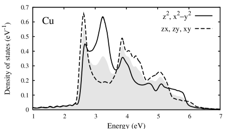
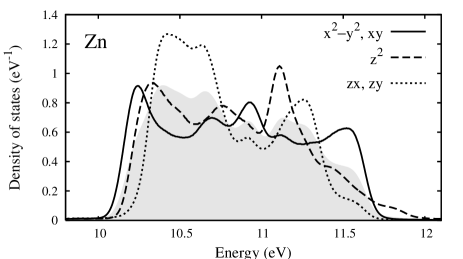
Figure 2: One-hole local density of states, $d(\omega)$, for Cu (top) and Zn (bottom), relative to the Fermi energy and normalized to unity. The shaded area is the total $d$ DOS, $\bar{d}$.

As a final ingredient, Table 3 lists the values of $U$ for the five $LS$ components of the multiplet, computed by Eq. (14). Notice that the inclusion of a $q$ dependence in $U$ (via a cubic term in the expansion of the total energy with respect to a fractional charge) proves to be quite important. Indeed, in evaluating $U$ the $C$ coefficient is counted six times, hence bringing a larger contribution than in the XPS energies previously discussed. Such inclusion gives an estimate of $U=U(q=1)$ which is $0.60$ eV and $2.52$ eV larger for Cu and Zn, respectively, than the corresponding values obtained as $U(q=0)$.

	$U_{\text{sph}}$	${}^{1}S$	${}^{1}G$	${}^{3}P$	${}^{1}D$	${}^{3}F$
Cu	2.38	7.76	3.34	2.67	2.25	0.33
Zn	8.16	14.31	9.26	8.49	8.01	5.82

Table 3: Values of $U$ resulting from the application of Eq. (14), in eV. Slater’s integrals from Ref. Antonides et al., 1977.

We then compute the $L_{23}M_{45}M_{45}$ Auger spectrum following Eq. (4). The outcome has been convoluted with a core hole lifetime of $0.49$ and $0.27$ eV ($0.42$ and $0.33$ eV)Yin et al. (1973) for the $L_{2}$ and $L_{3}$ lines of Cu (Zn), respectively, and results in a multiplet of generally narrow atomic-like peaks, shown in Fig. 3.

To analyze these results, let us focus on the principal peak (${}^{1}G$) in the spectrum, which can be associated with the absolute position of the multiplet. (The internal structure of the multiplet in our description only depends on the values of $F^{2}$ and $F^{4}$ which, as previously specified, were taken from the literature.) The experimental energy of the (most intense) ${}^{1}G$ transitionAntonides et al. (1977) is marked by a vertical line in Fig. 3. The agreement of our results is rather good considering the absence of adjustable parameters in the theory: focusing on the $L_{3}VV$ line, the ${}^{1}G$ peak position ($918.0$ eV from experiments) is overestimated by $1.6$ eV, while the one for Zn ($991.5$ eV) is underestimated by $1.9$ eV.

Figure 3: Simulated $L_{23}M_{45}M_{45}$ spectrum for Cu (top) and Zn (bottom) metals. The vertical lines mark the position of the principal (${}^{1}G$) peaks from experiments.Antonides et al. (1977)

IV Discussion

It is interesting to compare these results with those obtained by an expression commonly adopted for Auger energies, i.e., $\omega_{LS}\approx\epsilon_{c}-2\epsilon_{v}-U_{LS}$. This is an excellent approximation when $U$ is larger than $W$: for example in Zn, where $W\approx 1.5$ eV and $U_{{}^{1}G}=9.26$ eV, its application to the computed parameters yields a value which is only $0.10$ eV larger than the ${}^{1}G$ peak position derived from Eq. (4). However, when $U$ is of order of $W$, significant deviations can be observed: e.g., for Cu ($W\approx 3.5$ eV and $U_{{}^{1}G}=3.34$ eV) the ${}^{1}G$ position is overestimated by $0.66$ eV. For smaller values of $U$, the quasi-atomic peak is lost for a broad band-like structure. This is the case for the ${}^{3}F$ component of Cu (the rightmost shoulder in the spectrum) for which we obtain $U_{{}^{3}F}=0.33$ eV. However, this is an artifact of our underestimate of $U_{\text{sph}}$ in Cu: experimentally, the ${}^{3}F$ peak is resolved as well.

Besides these observations, the expression $\omega_{LS}\approx\epsilon_{c}-2\epsilon_{v}-U_{LS}$ is accurate enough for the ${}^{1}G$ peak to discuss the discrepancy of our results with respect to the experimental ones. Let us focus on the $L_{3}VV$ part of the spectrum, and decompose the Auger kinetic energy $\omega$ into its contributions (see Table 4). Despite the fact that the overall agreement is similar in magnitude for Cu and Zn, it is important to remark that this finding has different origins. In both metals, we underestimate slightly the core photoemission energy and overestimate the valence photoemission energy by a similar amount. Both effects contribute underestimating the kinetic energy. In Zn, where our value of $U$ is excellent, the error in $\omega$ stems from the errors in the photoemission energies. In Cu, instead, $U$ is seriously underestimated. This overcompensates the error in the photoemission energies, resulting in a fortuitous overall similar accuracy.

		$\epsilon_{c}$	$-2\epsilon_{v}$	$-U_{{}^{1}G}$	$\omega_{{}^{1}G}$
	Theory	$931.31$	$-7.67$	$-3.34$	$920.29$
Cu	Exp.	$932.2$	$-6.2$	$-8.0$	$918.0$
	Diff.	$-0.9$	$-1.5$	$4.7$	$2.3$
	Theory	$1020.26$	$-21.55$	$-9.26$	$989.45$
Zn	Exp.	$1020.9$	$-19.8$	$-9.5$	$991.5$
	Diff.	$-0.6$	$-1.8$	$0.2$	$-2.1$

Table 4: Decomposition of the ${}^{1}G$ $L_{3}M_{45}M_{45}$ Auger kinetic energy into its contributions, according to the simple approximation $\omega=\epsilon_{c}-2\epsilon_{v}-U$. Theoretical values of $\epsilon_{c}$, $\epsilon_{v}$, and $U$ from tables 2 and 3; experimental data from Ref. Antonides et al., 1977. Values in eV.

We now examine the relative weight of two different ingredients of our method. First, the role of the spin-orbit interaction in the final state, which will be analyzed by comparing with results where such term is neglected; second, the resolution of the 2hLDOS in its angular components. To this respect, we notice that the matrix expression for the spectrum given in Eq. (4) can be significantly simplified under the assumption that the 2hLDOS is spherically symmetric and the spin-orbit contribution can be neglected. In this case, we can just take the spherically averaged, i.e., the total $d$ 1hLDOS, and compute its self-convolution, $\bar{D}^{(0)}\equiv\bar{d}*\bar{d}$. An averaged Green’s function, $\bar{G}^{(0)}$, is then defined as the Hilbert transform of $\bar{D}^{(0)}$. By replacing $G^{(0)}_{LSJM_{J},L^{\prime}S^{\prime}J^{\prime}M_{J^{\prime}}^{\prime}}$ in Eq. (4) with the diagonal matrix $\delta_{LSJM_{J},L^{\prime}S^{\prime}J^{\prime}M_{J^{\prime}}^{\prime}}\bar{G}^{(0)}$, we obtain the simple scalar equation

$$S(\omega)=-\frac{1}{\pi}\sum_{LSJ}(2J+1)|A_{LS}|^{2}\text{Im}\left[\frac{\bar{G}^{(0)}(\epsilon_{c}-\omega)}{1-U_{LS}\bar{G}^{(0)}(\epsilon_{c}-\omega)}\right],$$ (15)

where the dependence on $LS$ quantum numbers is only via the matrix elements and the interaction matrix $U$, and each $LS$ component of the spectrum is decoupled from the others.

The Auger spectra simulated neglecting the spin-orbit interaction and calculated with the simplified expression of Eq. (15) are plotted in Fig. 4 as dashed and dotted line, respectively, to be compared with the result of the full calculation [Eq. (4)], solid line. For simplicity, we limit the discussion to the $L_{3}VV$ line of Zn. The resemblance of the three results is remarkable. Indeed, in Cu and Zn the spin-orbit splitting for $3d$ levels is relatively small, $0.27$ and $0.36$ eV, respectively.NIST Furthermore, despite the differences which characterize the angular components of the 1hLDOS (see Fig. 2), the convoluted 2hLDOS are only mildly different from $\bar{D}^{(0)}$, as reported in Fig. 5. Now, in systems with a large $U/W$ ratio, fine details of the 2hLDOS are not relevant for the position of quasi-atomic peaks, which only depend on the weighted averages $E^{(0)}_{LS}$ as in Eq. (5). In our case, the values of $E^{(0)}_{LS}$ lie within $0.1$ eV from those corresponding to the averaged 2hLDOS. Hence the practically equivalent results obtained by Eq. (4) and Eq. (15).

Figure 4: Simulated spectrum for the $L_{3}M_{45}M_{45}$ line of Zn. Solid line: full treatment of Eq. (4), as presented in this paper. Dashed line: neglecting the spin-orbit interaction in the two-hole final state. Dotted line: adopting the spherically averaged 2hLDOS and the scalar formulation, Eq. (15). The origin of the vertical axis is shifted for improved clarity.

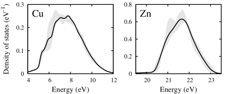
Figure 5: Non-interacting two-holes density of states, $D^{(0)}$, for Cu (left) and Zn (right). The solid curve represents $\bar{D}^{(0)}\equiv\bar{d}*\bar{d}$, the self-convolution of the total $d$ 1hLDOS; the shaded area indicates the largest deviations from this result found amongst the angular resolved 2hLDOSs.

This analysis shows that, for a wide class of systems with strong hole-hole interaction, weak spin-orbit interaction, and a spherical symmetry to some extent, the simple formulation presented in Eq. (15) is practically as accurate as the expression in Eq. (4). One should instead adopt the full treatment for, e.g., heavier elements, or systems with low dimensionality. This remark is independent of the methodology to determine the parameters entering the model, either fully ab initio as in the present approach, or by phenomenological arguments.

Our method provides an agreement with experimental photoemission energies of the order of $1$ eV and of $2$ eV for Auger energies. We consider this to be a rather good result, as a starting point, considering the absence of adjustable parameters in the model which is the new feature of our approach for CVV transitions in correlated systems. We trust that our simple method could already yield qualitative information on the variations of the spectrum to be expected following to modifications in the sample, e.g., when the emitting atom is located in different environments. Of course, a much better agreement would be obtained by inserting phenomenological parameters, but at the cost of loosing predictive power.

The internal structure of the lineshape, i.e., the multiplet splitting, is given very precisely. However, the first-principles treatment of the latter is not a new aspect of our approach, which is indeed based in this respect on atomic results available in the literature since decades. Let us instead focus again on the estimated position of the multiplet, which crucially depends on the parameters evaluated by our ab initio method. Even though the agreement with the experiment is about as good as for Zn as for Cu, actually the results for Zn are much better. In Zn, the $3d$ band is deep and narrow, and electronic states bear mostly atomic character. Their hybridization with the states closer to the Fermi level, which mainly contributes to screening, is small, somehow in an analogous way as for core states. Consequently, the approximations to neglect the energy dependence of $B_{v}$ and $C_{v}$, and to transfer the values of $\Delta{}B$ and $\Delta{}C$ from the core states to the valence ones, produce very good results. In Cu, instead, the $3d$ band is higher and broader, and hybridizes significantly with the $s$-like wavefunctions. Our approximations turn out to be less adequate: the resulting $U$ is about half the one derived from experiments.

Part of this discrepancy might also have a deeper physical origin, since the Hamiltonian adopted, Eq. (1), does not allow for the interaction amongst two holes located at different atomic sites. The CS model has been extended to consider the role of interatomic (“off-site”) correlation effects which mainly produce an energy shift of the Auger line to lower energies.Verdozzi (1995) Studies based on phenomenological parameters suggest that such an energy shift could be of about $2.5$ eV in CuUgenti et al. (2008) (smaller values are expected in Zn where holes are more localized and screening is more effective). For sake of simplicity, the off-site term has not been considered here and is left for future investigations. The parameters entering this term could be determined by ab initio methods in analogy to the procedure shown here for evaluating $U$. It is however important to notice that adding the off-site term would not fix all the discrepancies observed in Cu, where also the lineshape, in addition to the peak position, is not satisfactory owing to small values for the on-site interaction $U$ (e.g., the non-resolved ${}^{3}F$ peak).

Enhancing the accuracy of the values of $U$ seems therefore the most important improvement for the method presented here, especially for systems with broad valence bands. As a possibility, it would be interesting to use approaches which are capable to compute the total energy in presence of holes in the valence state. The methodology presented in Ref. Cococcioni and de Gironcoli, 2005, in which the valence occupation is changed by means of Lagrange multipliers associated with the KS eigenvalues, could be particularly effective. One should pay attention as some arbitrariness is anyway introduced. Namely, the value of $U$ does depend on the chosen form of the valence wavefunctions. Such an arbitrariness is compensated in LDA+U calculations performed self-consistently.Cococcioni and de Gironcoli (2005) Furthermore, to apply this method to systems with closed band lying well below the Fermi energy, large shifts of the KS eigenvalues would be needed to alter the occupation of the band to an appreciable amount.

Another possible improvement concerns the photoemission energies. Calculations by the $GW$ approachAryasetiawan and Gunnarsson (1998) of the 1hLDOS could be used to account for relaxation energies, rather than adopting Eq. (8). Results available in the literature (e.g., for Cu Marini et al. (2001)) are very promising in that sense. It is interesting to notice that the factor $B+C$ plays the role of a self-energy expectation value, and that the use of a single value of $B+C$ to shift rigidly the band is formally analogous to the “scissor operator” often introduced to avoid expensive self-energy calculations. The accuracy of such rigid shifts for valence-band photoemission in Cu is discussed in Ref. Marini et al., 2001.

Systems with larger band width or smaller hole-hole interaction would require to extend the approach to treat the dependence of the matrix elements on energy together with the interaction in the final state. Releasing the assumption that matrix elements equal the atomic ones, as in the current treatment, or that particles are non-interacting in formulations accounting for such an energy dependence (like, e.g., the one in Ref. Bonini et al., 2003), would allow switching continously between systems with band-like and atomic-like spectra. This possibility is currently under investigation.

Finally, let us recall the basic assumption considered here that the valence shell is closed, which is crucial to the CS model in its original form. Efforts have been devoted towards releasing this assumption, resulting in a formulation by more complicated three-hole Green’s functions,Marini and Cini (1999) for which no ab initio treatment is nowadays available to our knowledge.

V Conclusions

We have presented an ab initio method for computing CVV Auger spectra for systems with filled valence bands, based on the Cini-Sawatzky model. Only standard DFT calculations are required, resulting in a very simple method which allows working out the spectrum with no adjustable parameters. The accuracy on the absolute position of the Auger features is estimated to a few eV, as we have demonstrated by the analysis of Cu and Zn metals. We have shown that in these systems further simplifications like neglecting spin-orbit interaction for the two valence holes, or the non sphericity of the emitting atom, give results practically equivalent to the full treatment. Attention should be paid to the problematic parameter $U$. We obtained such a term with a good accuracy for the more localized, atomic-like valence bands in Zn, while it results underestimated in Cu. Its occupation number dependence, included via a cubic term in the expansion of the total energy, has been considered, and shown to play an important role.

This step towards a first-principles description of CVV spectroscopy in closed-shell correlated systems enables identifying improvements which future investigations could focus on. In particular, one would benefit from detailed calculations of the single-particle densities of states (e.g., by the $GW$ method), from truly varying the valence-band occupation to obtain the $U$ parameter, and from including off-site terms in the Hamiltonian. Prospectively, it would be desirable to take into account the energy dependence of the transition matrix elements.

VI Acknowledgment

This work was supported by the MIUR of Italy (Grant No. 2005021433-003) and the EU Network of Excellence NANOQUANTA (Grant No. NMP4-CT-2004-500198). Computational resources were made available also by CINECA through INFM grants. EP is financially supported by Fondazione Cariplo (n. Prot. 0018524).

References

- Verdozzi et al. (2001) C. Verdozzi, M. Cini, and A. Marini, J. Electron Spectrosc. Relat. Phenom. 117, 41 (2001).
- Gunnarsson and Schönhammer (1980) O. Gunnarsson and K. Schönhammer, Phys. Rev. B 22, 3710 (1980).
- Cini (1977) M. Cini, Solid State Commun. 24, 681 (1977).
- Sawatzky (1977) G. A. Sawatzky, Phys. Rev. Lett. 39, 504 (1977).
- Cini and Drchal (1995) M. Cini and V. Drchal, J. Electron Spectrosc. Relat. Phenom. 72, 151 (1995).
- Cole et al. (1994) R. J. Cole, C. Verdozzi, M. Cini, and P. Weightman, Phys. Rev. B 49, 13329 (1994).
- Verdozzi and Cini (1995) C. Verdozzi and M. Cini, Phys. Rev. B 51, 7412 (1995).
- Verdozzi (1995) C. Verdozzi, J. Electron Spectrosc. Relat. Phenom. 72, 141 (1995).
- Anisimov et al. (1991) V. I. Anisimov, J. Zaanen, and O. K. Andersen, Phys. Rev. B 44, 943 (1991).
- Anisimov et al. (1993) V. I. Anisimov, I. V. Solovyev, M. A. Korotin, M. T. Czyżyk, and G. A. Sawatzky, Phys. Rev. B 48, 16929 (1993).
- Hubbard (1963) J. Hubbard, Proc. Roy. Soc. A 276, 238 (1963).
- Antonides et al. (1977) E. Antonides, E. C. Janse, and G. A. Sawatzky, Phys. Rev. B 15, 1669 (1977).
- Gunnarsson et al. (1989) O. Gunnarsson, O. K. Andersen, O. Jepsen, and J. Zaanen, Phys. Rev. B 39, 1708 (1989).
- Janak (1978) J. F. Janak, Phys. Rev. B 18, 7165 (1978).
- Slater (1960) J. C. Slater, Quantum Theory of the Atomic Structure (McGraw-Hill, New York, 1960).
- Anisimov and Gunnarsson (1991) V. I. Anisimov and O. Gunnarsson, Phys. Rev. B 43, 7570 (1991).
- Shirley (1973) D. A. Shirley, Phys. Rev. A 7, 1520 (1973).
- Pickett et al. (1998) W. E. Pickett, S. C. Erwin, and E. C. Ethridge, Phys. Rev. B 58, 1201 (1998).
- Cococcioni and de Gironcoli (2005) M. Cococcioni and S. de Gironcoli, Phys. Rev. B 71, 035105 (2005).
- Perdew et al. (1996) J. P. Perdew, K. Burke, and M. Ernzerhof, Phys. Rev. Lett. 77, 3865 (1996).
- (21) NIST, Atomic reference data for electronic structure calculations, http://physics.nist.gov/PhysRefData/DFTdata/.
- Yin et al. (1973) L. I. Yin, I. Adler, M. H. Chen, and B. Crasemann, Phys. Rev. A 7, 897 (1973).
- Ugenti et al. (2008) S. Ugenti, M. Cini, E. Perfetto, F. D. Pieve, C. Natoli, R. Gotter, F. Offi, A. Ruocco, G. Stefani, F. Tommasini, et al., J. Phys.: Conf. Series 100, 072020 (2008).
- Aryasetiawan and Gunnarsson (1998) F. Aryasetiawan and O. Gunnarsson, Rep. Prog. Phys. 61, 237 (1998).
- Marini et al. (2001) A. Marini, G. Onida, and R. DelSole, Phys. Rev. Lett. 88, 016403 (2001).
- Bonini et al. (2003) N. Bonini, G. P. Brivio, and M. I. Trioni, Phys. Rev. B 68, 035408 (2003).
- Marini and Cini (1999) A. Marini and M. Cini, Phys. Rev. B 60, 11391 (1999).