Rescaled Lévy-Loewner hulls and random growth

Abstract.

We consider radial Loewner evolution driven by unimodular Lévy processes. We rescale the hulls of the evolution by capacity, and prove that the weak limit of the rescaled hulls exists. We then study a random growth model obtained by driving the Loewner equation with a compound Poisson process. The process involves two real parameters: the intensity of the underlying Poisson process and a localization parameter of the Poisson kernel which determines the jumps. A particular choice of parameters yields a growth process similar to the Hastings-Levitov $\rm{HL}(0)$ model. We describe the asymptotic behavior of the hulls with respect to the parameters, showing that growth tends to become localized as the jump parameter increases. We obtain deterministic evolutions in one limiting case, and Loewner evolution driven by a unimodular Cauchy process in another. We show that the Hausdorff dimension of the limiting rescaled hulls is equal to $1$. Using a different type of compound Poisson process, where the Poisson kernel is replaced by the heat kernel, as driving function, we recover one case of the aforementioned model and $\rm{SLE}(\kappa)$ as limits.

1. Introduction and main results

1.1. Introduction

The Loewner differential equation was first derived by Loewner in 1923 in a paper on coefficient problems for univalent functions and has proved to be one of the most powerful tools in the theory of univalent functions. This differential equation parametrizes functions mapping conformally onto various reference domains (usually the unit disk or the upper half-plane) minus a single slit in terms of a continuous unimodular function. On the other hand, given a unimodular function (which will be called driving function in this context), one obtains from the Loewner equation a univalent function, which needs not be a single-slit mapping.

Loewner’s equation has also proved to be of use in mathematical physics. For instance, in the paper [CM01], Carleson and Makarov use the Loewner equation to study a model related to Diffusion Limited Aggregation (DLA). In the last few years, solutions to the Loewner equation corresponding to random driving functions have attracted a great amount of interest in mathematics as well as physics. For instance, if standard Brownian motion on the unit circle is chosen as driving function, one obtains Schramm-Loewner evolution or SLE for short. SLE arises naturally in connection with scaling limits of various discrete models from statistical physics and provides a tool to treat many aspects of that field rigorously. We refer the reader to the book [Law05] and the paper [RS05] for basic results on SLE. Recently, the Loewner equation together with other, more general, stochastic processes has attracted some interest, see [CR07] and the references therein.

1.2. Main results

Our paper is organised as follows. Beginning in Section 3 we consider the Loewner equation driven by general Lévy processes. This yields a family of conformal maps mapping the exterior disk onto the complements of a family of growing compact connected sets, the so-called hulls of the evolution. We take on the view of the Loewner equation as a mapping from the Skorokhod space of right-continuous functions with left limits, and establish the continuity of this mapping in Proposition 3.1. We rescale the compacts by capacity and by using reversibility of Lévy processes, we prove a form of convergence of the rescaled hulls in Theorem 3.3.

In the final section, we study evolutions corresponding to a particular choice of Lévy process of pure jump type involving two real parameters $r$ and $\lambda$. We consider random variables $X^{r}$ with densities proportional to harmonic measure at different points whose distance to the growing cluster is controlled by $r$. The variables are then added at the occurrence times of a Poisson process with intensity $\lambda$. For the particular choice $r=0$ (corresponding to harmonic measure at the point at infinity), the evolution we obtain resembles the Hastings-Levitov model $\rm{HL}(0)$ in Laplacian growth and may be viewed as a random perturbation of that model. We study our models’ dependence on the parameters, and show that the hulls we obtain become more regular with increasing $r$ (which corresponds to moving the base points of harmonic measure closer to the hull) in the sense that the growth becomes more localized and the hulls tend to grow fewer large branches. In the limit, with $\lambda$ fixed, we obtain deterministic hulls, see Proposition 4.1. Another passage to the limit (which involves both parameters) yields Loewner evolution driven by the Cauchy process, see Proposition 4.3. The hulls generated by this process still exhibit branching behavior. Replacing the Poisson kernel as the density of the variables $X^{r}$ by the heat kernel of the circle, which is more localized, we obtain Schramm-Loewner evolution $\rm{SLE}(\kappa)$ in a particular limiting case that involves both the intensity of the Poisson process and the localization parameter of the heat kernel. At the other extreme, when the heat kernel becomes spread out on the circle, we recover the perturbed Hastings-Levitov model. Finally, in Theorem 4.4, we show that the Hausdorff dimension of the scaling limit of the hulls (in the sense of Theorem 3.3) is $1$ for all $r$ and large enough $\lambda$, as is the case in the $\rm{HL}(0)$ model.

2. Preliminaries

2.1. The Loewner equation and classes of conformal mappings

Let $\mathbb{D}$ denote the unit disk and let $\xi$ be a function of the real variable $t$ taking values on the unit circle. The radial version of Loewner’s equation is

(2.1) $$\partial_{t}g_{t}(z)=g_{t}(z)\frac{\xi(t)+g_{t}(z)}{\xi(t)-g_{t}(z)},\quad\textrm{with}\quad g_{0}(z)=z,$$

for $0\leq t<\infty$. For each $z\in\mathbb{D}$, the equation (2.1) is well-defined up to

$$\tau_{z}=\sup\{t:\inf_{0\leq s\leq t}|g_{s}(z)-\xi(s)|>0\},$$

that is, the first time the denominator in the right-hand side of (2.1) is zero. We let

(2.2) $$K_{t}=\{z:\tau_{z}\leq t,\,z\in\mathbb{D}\}$$

denote the growing compact hulls. It is well-known that there exists a unique solution $g_{t}$ to (2.1) if $\xi$ is integrable (see [Dur83, Section 3.4] for a general discussion). For each $t$, the function $g_{t}$ is a conformal map from $\mathbb{D}\setminus K_{t}$ onto $\mathbb{D}$.

We note that $g_{t}$ fixes the origin and that $g^{\prime}_{t}(0)=e^{t}$. Often, it is the inverse of $g_{t}$, that is, the conformal map of $\mathbb{D}$ onto $\mathbb{D}\setminus K_{t}$, that we would like to study. This function may be obtained as the solution of a partial differential equation (with given initial value) involving the driving function, namely,

(2.3) $$\partial_{t}f_{t}(z)=z\partial_{z}f_{t}(z)\frac{z+\xi(t)}{z-\xi(t)},\quad f_{0}(z)=z.$$

Next, let

$$\Delta=\{z\in\mathbb{C}_{\infty}:|z|>1\},$$

be the exterior of the unit disk. It is easily verified that the map $g^{*}_{t}=1/g_{t}(1/z)$ also satisfies (2.1), this time with driving function $\overline{\xi}$. The solution $g^{*}_{t}$ maps $\Delta\setminus K_{t}^{*}$ conformally onto $\Delta$, where

$$K_{t}^{*}=\{z:1/z\in K_{t}\}.$$

We note that $g^{*}_{t}$ has an expansion of the form

$$g^{*}_{t}(z)=e^{-t}z+\cdots$$

at infinity. Again, we obtain the inverse mappings by solving the partial differential equation (2.3). Hence, the equations (2.1) and (2.3) can be used to describe growing hulls both in $\mathbb{D}$ and $\Delta$. In this paper, we consider evolutions in the exterior disk.

One may also consider the equation (2.1) in the exterior disk for negative $t$. This leads to the notion of whole-plane Loewner evolution. More precisely, for a driving function $\varphi$ defined for $-\infty<t<\infty$, we consider solutions of

(2.4) $$\partial_{t}g_{t}(z)=g_{t}(z)\frac{\varphi(t)+g_{t}(z)}{\varphi(t)-g_{t}(z)},$$

with initial condition

(2.5) $$\quad\lim_{t\to-\infty}e^{t}g_{t}(z)=z.$$

The associated hulls, defined in the same manner as before, grow from the origin and become arbitrarily large as $t\to\infty$. As in the previous cases, the inverse mappings $f_{t}$ satisfy the related partial differential equation

(2.6) $$\partial_{t}f_{t}(z)=z\partial_{z}f_{t}(z)\frac{z+\varphi(t)}{z-\varphi(t)},$$

with initial condition

(2.7) $$\lim_{t\rightarrow-\infty}e^{-t}f_{t}(z)=z.$$

We shall occasionally refer to these different Loewner equations by using the prefixes $\mathbb{D},\,\Delta$, and $\mathbb{C}$.

We have seen that the Loewner equation generates conformal mappings, and we now set down some notation for the different classes of mappings that arise. The class $\mathcal{S}$ consists of univalent functions $f:\mathbb{D}\rightarrow\mathbb{C}$ with power series expansions of the form

$$f(z)=z+\sum_{n=2}^{\infty}a_{n}z^{n}.$$

These functions map the unit disk onto simply connected domains containing the origin. The Loewner equation was in fact first introduced in connection with coefficient problems for $\mathcal{S}$. Next, we let $\Sigma$ denote the class of univalent functions $f$ in $\Delta$ with expansions at infinity of the form

$$f(z)=z+b_{0}+\sum_{n=1}^{\infty}\frac{b_{n}}{z^{n}}.$$

A function in $\Sigma$ maps the exterior disk onto the complement of a compact simply connected set. Finally, the subclass $\Sigma^{\prime}$ consists of those $f\in\Sigma$ whose omitted set contains the origin. We note that $\mathcal{S}$ and $\Sigma^{\prime}$ are related via the inversion mapping discussed earlier. We endow the classes $\mathcal{S}$ and $\Sigma$ with the topology induced by uniform convergence on compact subsets. We note that $\Sigma^{\prime}$ is compact with respect to this topology. We refer the reader to [Dur83] for a thorough treatment of univalent functions.

2.2. Lévy processes and Skorokhod space

A (real-valued) stochastic process $X=(X(t))_{t\in[0,\infty)}$ defined on some probability space $(\Omega,\mathcal{F},\mathbb{P})$ is said to be a Lévy process if $X(0)=0$ almost surely, if the process has independent and stationary increments, and if, for all $\epsilon>0$, it holds that

$$\lim_{t\rightarrow 0}\mathbb{P}(|X(t)|>\epsilon)=0.$$

Clearly, standard Brownian motion is an example of a Lévy process. The Poisson process and compound Poisson processes provide us with additional examples of Lévy processes. It is well-known that the sample paths of standard Brownian motion are continuous almost surely. The sample paths of general Lévy processes do not have this property. It is true, however, that the sample paths of a Lévy process are right-continuous with left limits (RCLL) (more precisely, any Lévy process admits a modification with these properties).

There is a natural topology, known as the Skorokhod topology, on spaces of RCLL functions on the real line. Let us first consider the case of Skorokhod spaces on an interval $[0,T]$. The class $\Lambda=\Lambda[0,T]$ consists of continuous non-decreasing functions on $[0,T]$ with $\lambda(0)=0$ and $\lambda(T)=T$. We set

(2.8) $$\|\lambda\|_{\Lambda}=\sup_{s\neq t}\left|\log\left(\frac{\lambda(t)-\lambda(s)}{t-s}\right)\right|.$$

The Skorokhod metric on $D[0,T]$, the space of real-valued RCLL functions on $[0,T]$, is then given by

(2.9) $$d(\varphi,\psi)=\inf\{\epsilon>0:\exists\lambda\,\,\textrm{such that}\,\,\|\varphi-\psi\circ\lambda\|_{\infty}<\epsilon,\|\lambda\|_{\Lambda}<\epsilon\}.$$

The space $D[0,T]$ is a complete and separable metric space when equipped with this metric. Note that the restriction of $d$ to the subspace of continuous functions induces the usual uniform topology on $C[0,T]$. The following lemma (see [Bil68]) shows that the functions in $D[0,T]$ are reasonably well-behaved:

Lemma 2.1.

For each $\epsilon>0$ and $\varphi\in D[0,T]$ there exist a finite number $N=N(\epsilon)$ of points $0=t_{0}<t_{1}\cdots<t_{N}=T$ such that

$$\sup\{|\varphi(s)-\varphi(t)|:s,t\in I_{j}\}<\epsilon$$

for $j=0,1,\ldots N-1$ and $I_{j}=[t_{j},t_{j+1})$.

We see that Skorokhod functions can have at most a countable number of discontinuities. The above lemma, together with the fact that $\|\lambda\|_{\Lambda}<\epsilon$ implies $\|\lambda-t\|_{\infty}<2T\epsilon$, can be used to show that convergence in $D[0,T]$ in the Skorokhod metric implies convergence in $L^{1}[0,T]$. In fact, using that a function in $D[0,T]$ can be approximated uniformly by a finite step function, one can prove the following stronger result (we omit the details).

Lemma 2.2.

For each $\epsilon>0$ and each $\varphi\in D[0,T]$, there exists a $\delta>0$ such that $d(\varphi,\psi)<\delta$ implies that for all $t\in[0,T]$,

$$\int_{0}^{t}|\varphi(s)-\psi(s)|ds<\epsilon t.$$

We often wish to consider the space $D[0,\infty)$ of RCLL functions on the real line. The Skorokhod topology is defined as follows in this case (see [JS87]). We say that a sequence $\{\varphi_{i}\}_{i=1}^{\infty}$ of functions in $D[0,\infty)$ converges to $\varphi\in D[0,\infty)$ if there is a sequence of continuous, strictly increasing functions $\{\lambda_{i}\}_{i=1}^{\infty}$ such that $\lambda_{i}(0)=0$, $\lambda_{i}(t)\rightarrow\infty$ as $t\rightarrow\infty$, and

(2.10) $$\left\{\begin{array}[]{c}\sup_{t\in[0,\infty)}|\lambda_{i}(t)-t|\rightarrow 0\\ \sup_{t\leq N}|\varphi_{i}(\lambda_{i}(t))-\varphi(t)|\rightarrow 0,\quad\forall N\in\mathbb{N}.\end{array}\right.$$

The Skorokhod topology on $D(-\infty,0]$ is defined in an analogous manner.

We will need the following lemma which is contained in [JS87, Corollary VII.3.6].

Lemma 2.3.

Let $(X_{n}(t))_{t\in[0,\infty)}$ and $(X(t))_{t\in[0,\infty)}$ be Lévy processes. Then, as $n\to\infty$, the law of $X_{n}$ converges weakly to that of $X$ in the space of probability measures on $D[0,\infty)$ if and only if the random variables $X_{n}(1)$ converge in distribution to $X(1)$.

We refer the reader to [Ber96] for more background information on Lévy processes. The Skorokhod space is treated in depth in [JS87].

Throughout this paper, we shall always assume that probability measures are defined on the appropriate Borel sigma algebra. For a metric space $S$, we let $\Pi(S)$ denote the space of Borel probability measures on $S$ with the topology induced by weak convergence.

3. Rescaled Loewner evolution driven by Lévy processes

This section is dedicated to the study of Loewner evolution driven by general Lévy processes, and we establish several facts that we shall use later on in a more specific setting. The main result of this section is the weak convergence of Loewner evolution driven by Lévy processes after rescaling by capacity.

3.1. Continuity of the Loewner mapping

Let $D_{\mathbb{T}}[0,\infty)$ denote the space of unimodular RCLL functions on $[0,\infty)$, equipped with the Skorokhod topology. The space $L^{1}_{\mathbb{T}}[0,T]$ consists of all measurable unimodular functions on $[0,T]$. We note that any function in $D_{\mathbb{T}}[0,\infty)$ belongs to $L^{1}_{\mathbb{T}}[0,T]$ for any choice of $T$.

Consider the time $t=T$ solution $f_{T}$ to the $\Delta$-Loewner equation (2.6) with driving function $\varphi\in L^{1}_{\mathbb{T}}[0,\infty)$ and initial condition $f_{0}(z)=z$. We define a mapping

(3.1) $$\mathcal{L}_{T}:L^{1}_{\mathbb{T}}[0,T]\rightarrow\Sigma^{\prime}$$

by setting

(3.2) $$\mathcal{L}_{T}[\varphi](z)=e^{-T}f_{T}(z).$$

Usually, we shall consider the mapping $\mathcal{L}_{T}$ restricted to the Skorokhod space $D_{\mathbb{T}}[0,\infty)$. We next show that the mappings $\mathcal{L}_{T}$ are well-behaved.

Proposition 3.1.

For each $T>0$, the Loewner mapping

$$\mathcal{L}_{T}:L^{1}_{\mathbb{T}}[0,T]\rightarrow\Sigma^{\prime}$$

is continuous.

We will follow the approach of Bauer. He obtains similar results for the chordal Loewner equation viewed as a mapping from $C[0,\infty)$, with the uniform topology, to a certain space of conformal mappings of the upper half-plane (see [Bau03] for details; see also [Dur83, Section 3.4]).

Proof of Proposition 3.1.

It is well-known (see for instance [Law05, Section 4.2]) that the conformal mapping $f_{T}$ can be obtained by considering the backward flow

$$\partial_{t}h_{t}(z)=-h_{t}(z)\frac{\varphi(T-t)+h_{t}(z)}{\varphi(T-t)-h_{t}(z)},\quad h_{0}(z)=z$$

for $0\leq t\leq T$, and we have $\mathcal{L}_{T}[\varphi](z)=e^{-T}h_{T}(z)$. In what follows, we set

$$v(t,\varphi,z)=-z\frac{\varphi(T-t)+z}{\varphi(T-t)-z}.$$

With this notation, the equation determining the backward flow becomes

(3.3) $$\partial_{t}h_{t}(z)=v(t,\varphi,h_{t}(z)),\quad h_{0}(z)=z.$$

Let $\epsilon>0$ be given, and suppose $\varphi,\psi\in L^{1}_{\mathbb{T}}[0,T]$. We fix $z\in\Delta$ with $z=re^{i\theta}$, and we let $u_{1}=u_{1}(t)$ denote the solution to (3.3) with $\varphi$ as driving function. Similarily, we let $u_{2}$ denote the solution corresponding to $\psi$. Moreover, we write $\dot{u}_{i}$ for the derivative of $u_{i}$ with respect to $t$. We now show that $u_{2}$ is an approximate solution to $\dot{u}_{1}(t)=v(t,\varphi,u_{1})$.

We compute that

$$\dot{u}_{2}(t)-v(t,\varphi,u_{2})=-2u_{2}^{2}(t)\frac{\varphi(T-t)-\psi(T-t)}{(\varphi(T-t)-u_{2}(t))(\psi(T-t)-u_{2}(t))}.$$

An integration then yields

$$\left|u_{2}(t)-u_{2}(0)-\int_{0}^{t}v(s,\varphi,u_{2})ds\right|\\ \leq 2\int_{0}^{t}|u_{2}(s)|^{2}\frac{|\varphi(T-s)-\psi(T-s)|}{|\varphi(T-s)-u_{2}(s)||\psi(T-s)-u_{2}(s)|}ds.$$

Standard growth estimates show that $|u_{2}(s)|\leq 4e^{T}r$. Next, we calculate that

$$\frac{d}{ds}\textrm{Re}[\log u_{2}(s)]>0,$$

which means that points in $\Delta$ move away from the unit circle under the backward flow. This implies that

$$|\varphi(T-s)-u_{2}(s)|\geq|u_{2}(0)|-1=r-1,$$

and a similar estimate holds for the other factor. Using these estimates, we obtain

$$\left|u_{2}(t)-u_{2}(0)-\int_{0}^{t}v(s,\varphi,u_{2})ds\right|\\ \leq 32e^{T}\frac{r^{2}}{(r-1)^{2}}\int_{0}^{t}|\varphi(T-s)-\psi(T-s)|ds.$$

The integral on the right-hand side can be made arbitrarily small if the functions $\varphi$ and $\psi$ are chosen so that $\|\varphi-\psi\|_{1}\leq 1/32\,e^{-T}\epsilon$. We then get

$$\left|u_{2}(t)-u_{2}(0)-\int_{0}^{t}v(s,\varphi,u_{2})ds\right|\leq\frac{r^{2}}{(r-1)^{2}}\epsilon.$$

Noting that $u_{1}(0)=u_{2}(0)=z$, and that $u_{1}$ is an exact solution to the problem (3.3), we see that

$$|u_{1}(t)-u_{2}(t)|\leq\frac{r^{2}}{(r-1)^{2}}\epsilon+\int_{0}^{t}|v(s,\varphi,u_{1})-v(s,\varphi,u_{2})|ds.$$

We wish to estimate the integrand in terms of the difference $|u_{1}-u_{2}|$. A computation shows that

$$|\partial_{z}v(s,\varphi,z)|\leq\frac{(r+1)^{2}}{(r-1)^{2}},$$

and we obtain that

$$|u_{1}(t)-u_{2}(t)|\leq\frac{r^{2}}{(r-1)^{2}}\epsilon+\frac{(4e^{T}r+1)^{2}}{(r-1)^{2}}\int_{0}^{t}|u_{1}(s)-u_{2}(s)|ds$$

Finally, an application of Grönwall’s lemma shows that

$$|u_{1}(t)-u_{2}(t)|\leq\frac{r^{2}}{(r-1)^{2}}\exp\left\{\frac{(4e^{T}r+1)^{2}}{(r-1)^{2}}T\right\}\cdot\epsilon.$$

We see that this estimate is uniform for $z=re^{i\theta}$ confined to an arbitrary compact set in $\Delta$. Since $|u_{1}(T)-u_{2}(T)|=|\mathcal{L}_{T}[\varphi](z)-\mathcal{L}_{T}[\psi](z)|$, the proof is now complete. ∎

We recall that convergence in the Skorokhod topology on $[0,\infty)$ implies convergence in $L^{1}{[0,T]}$ and obtain the following corollary.

Corollary 3.2.

For each $T>0$, the Loewner mapping

$$\mathcal{L}_{T}:D_{\mathbb{T}}[0,\infty)\rightarrow\Sigma^{\prime}$$

is continuous.

3.2. Weak convergence of rescaled hulls

Let $X=(X(t))_{t\in[0,\infty)}$ be a Lévy process and let $U$ be a uniformly distributed random variable on the unit circle, independent of $X$. We introduce a driving function for the $\Delta$-Loewner equation by setting

(3.4) $$\xi(t)=Y(t)=\exp\{i(U+X(t))\},\quad t\in[0,\infty).$$

We then let $f_{t}$, $t>0$, be the solution to (2.6) with driving function $\xi(t)$.

In this section we study rescalings of the hulls $K_{t}=\mathbb{C}\setminus f_{t}(\Delta)$. Recall that the capacity of the hulls $K_{t}$ is given by $\textrm{cap}(K_{t})=e^{t}$. In view of our application below is natural to normalize the hulls so that they have capacity $1$ for each $t$; this also means the diameter of the hulls stays bounded (both from above and away from $0$). We therefore introduce the rescaled hulls

(3.5) $$\tilde{K}_{t}=\frac{1}{\textrm{cap}(K_{t})}K_{t}=e^{-t}K_{t}.$$

On the level of mappings, this normalization places the conformal mapping $\tilde{f}_{t}$ of $\Delta$ onto $\mathbb{C}\setminus\tilde{K}_{t}$ in the class $\Sigma^{\prime}$. Let $\mathbb{P}_{t}$ denote the law of $\tilde{f}_{t}$.

Theorem 3.3.

We have

$$\mathbb{P}_{t}\rightarrow\mathbb{P}_{\infty},$$

as $t\to\infty$ in the sense of weak convergence of probability measures on $\Sigma^{\prime}$.

The limiting measure $\mathbb{P}_{\infty}$ will correspond to a whole-plane Loewner evolution evaluated at $t=0$.

Our approach requires that we introduce a suitable driving function for negative $t$. This involves time-reversal of the driving Lévy process.

In general, Lévy processes are reversible in the following sense. Suppose $V$ is a Lévy process on $[0,T]$. We define the time-reversed process $(\check{V}(t))_{t\in[0,T]}$ by setting

(3.6) $$\check{V}(t)=\left\{\begin{array}[]{cc}0&t=0\\ V((T-t)-)-V(T-)&0<t<T\\ -V(T-)&t=T\end{array}.\right.$$

Here we use the notation $V(s-)$ for the left-limit of $V$ at the point $s$. The process $(\check{V}(t))_{t\in[0,T]}$ is again a Lévy process and has the distribution of $(-V(t))_{t\in[0,T]}$ (see [JP88] for details).

Since we work with Lévy processes on the unbounded interval $[0,\infty)$, we will need to slightly modify the construction above in order to obtain a suitable driving process for negative $t$: Let $X$ be a given Lévy process on $[0,\infty)$ with law $\mu:=\mu_{X}\in\Pi(D[0,\infty))$. We define a reflected and time reversed process $\check{X}=(\check{X}(t))_{t\in(-\infty,0]}$, by setting

(3.7) $$\check{X}(t)=\left\{\begin{array}[]{cc}0&t=0\\ -X((-t)-)&t<0\end{array}.\right.$$

We view $\check{X}$ as a random element of the space $D(-\infty,0]$, with law $\check{\mu}:=\mu_{\check{X}}\in\Pi(D(-\infty,0])$.

Lemma 3.4.

Fix $T>0$ and let $X_{1}$ and $X_{2}$ be independent Lévy processes with laws $\mu\in\Pi(D[0,\infty))$ and $\check{\mu}\in\Pi(D(-\infty,0])$ respectively. Let $U_{1}$ and $U_{2}$ be two random variables uniformly distributed on $[-\pi,\pi]$, chosen independently of each other, as well as $X_{1}$ and $X_{2}$. Then the two processes

$$Y_{1}(t):=\exp\{i(U_{1}+X_{1}(t)\},\quad 0\leq t\leq T$$

and

$$Y_{2}(t):=\exp\{i(U_{2}+X_{2}(t-T))\},\quad 0\leq t\leq T$$

have the same law as elements of $D_{\mathbb{T}}[0,T]$.

Proof.

By reversibility, on $[0,T)$, it holds that

$$X_{1}(\cdot) \stackrel{{\scriptstyle d}}{{=}} -(X_{1}((T-\cdot)-)-X_{1}(T-)),$$

and hence on $[0,T)$

$$Y_{1}(\cdot) \stackrel{{\scriptstyle d}}{{=}} \exp\{i[U_{1}-\{X_{1}((T-\cdot)-)-X_{1}(T-)\}]\}$$

$$\stackrel{{\scriptstyle d}}{{=}} \exp\{i(U_{2}-X_{1}((T-\cdot)-))\}.$$

However, on $[0,T)$ we have

$$\exp\{i(U_{2}-X_{1}((T-\cdot)-))\} \stackrel{{\scriptstyle d}}{{=}} \exp\{i(U_{2}+X_{2}(\cdot-T))\}$$

$$= Y_{2}(\cdot),$$

and since $X_{2}(0)=0$ almost surely, this implies that the processes are equally distributed on the whole interval. ∎

We keep the notation of the previous lemma and let $\nu\in\Pi(D_{\mathbb{T}}[0,\infty))$ and $\check{\nu}\in\Pi(D_{\mathbb{T}}(-\infty,0])$ denote the laws of $Y_{1}$ and $Y_{2}$ respectively. We let $K_{t}$ denote the hulls corresponding to $Y_{1}$.

Recall that $\mathcal{L}_{t}$ is continuous for each $t\geq 0$, and that $\mathbb{P}_{t}$ is the law of the unique map $f_{t}\in\Sigma^{\prime}$ such that $e^{-t}K_{t}=\mathbb{C}\setminus f_{t}(\Delta)$. It follows that the family of probability measures $(\mathbb{P}_{t})_{t\in[0,\infty)}$ on the class $\Sigma^{\prime}$ can be written

$$\mathbb{P}_{t}=\nu\circ\mathcal{L}_{t}^{-1}.$$

We define a mapping $L_{\infty}:D_{\mathbb{T}}(-\infty,0]\rightarrow\Sigma^{\prime}$ by evaluating the solution to the whole-plane Loewner equation at $t=0$. An important step in the proof of Theorem 3.3 below is to show that $L_{\infty}$ is continuous on $D_{\mathbb{T}}(-\infty,0]$, so that the composition

$$\mathbb{P}_{\infty}=\check{\nu}\circ L_{\infty}^{-1}$$

is another probability measure on $\Sigma^{\prime}$.

Proof of Theorem 3.3.

We shall use the notation

$$w(t,\varphi,z;f):=z\partial_{z}f_{t}(z)\frac{z+\varphi(t)}{z-\varphi(t)}$$

for the right hand side of the Loewner partial differential equation. Let $\{t_{n}\}_{n=0}^{\infty}$ be an increasing sequence such that $t_{0}=0$ and $t_{n}\to\infty$ as $n\to\infty$. We write $\mathbb{P}_{n}:=\mathbb{P}_{t_{n}}$.

For an arbitrary $\varphi\in D_{\mathbb{T}}(-\infty,0]$, we let $f^{n}_{t}$ be the (unique) solution to $\partial_{t}f^{n}_{t}=w(t,\varphi,z;f^{n})$ for $-t_{n}<t\leq 0$ with the initial value $f^{n}_{-t_{n}}(z)=e^{-t_{n}}z$, and we set

$$L_{n}[\varphi]:=f^{n}_{0}.$$

It is easy to see, using the same arguments as in the previous section, that the mappings $L_{n}$ are continuous on $D_{\mathbb{T}}(-\infty,0]$, so that $\check{\nu}\circ L_{n}^{-1}$ is a probability measure. In view of Lemma 3.4, we then have $\check{\nu}\circ L_{n}^{-1}=\nu\circ\mathcal{L}_{t_{n}}^{-1}$ so that we may write $\mathbb{P}_{n}=\check{\nu}\circ L_{n}^{-1}$. Hence, the rescaled hull $\tilde{K}_{n}:=e^{-t_{n}}K_{t_{n}}$ has the distribution of $\mathbb{C}\setminus f(\Delta)$, where $f$ is chosen according to $\check{\nu}\circ L_{n}^{-1}$.

We will now show that $\{L_{n}\}$ converges uniformly on $D_{\mathbb{T}}(-\infty,0]$. Fix some compact $E\subset\Delta$ and take $m>n$ so that $t_{m}<t_{n}$. Let $\varphi\in D_{\mathbb{T}}(-\infty,0]$ be arbitrary and let $h_{t}^{n}$ solve

$$\partial_{t}h_{t}^{n}=w(t,\varphi,z;h^{n}),\quad-t_{n}<t\leq 0,$$

with initial value

$$h_{-t_{n}}^{n}(z)=z.$$

Keeping our previous notation, we denote by $f_{t}^{m}$ the solution to $\partial_{t}f_{t}^{m}=w(t,\varphi,z;f^{m})$ for $-t_{m}<t\leq 0$, with initial value $f_{-t_{m}}^{m}(z)=e^{-t_{m}}z$. Using a well-known property of solutions to the Loewner equation, we see that

$$L_{n}[\varphi]=e^{-t_{n}}z\circ h_{0}^{n},$$

and

$$L_{m}[\varphi]=f_{-t_{n}}^{m}\circ h_{0}^{n}.$$

We now apply [Law05, Lemma 4.20] in order to conclude that

$$\sup_{z\in E}|L_{n}[\varphi](z)-L_{m}[\varphi](z)|\leq C\cdot e^{-t_{n}},$$

for a constant $C<\infty$ independent of $\varphi$.

Thus, the sequence $L_{n}$ converges uniformly on $D_{\mathbb{T}}(-\infty,0]$ to the continuous map $L_{\infty}$, given by $L_{\infty}[\varphi]=f_{0}^{\infty}$, where $f_{t}^{\infty}$ solves

$$\partial_{t}f_{t}^{\infty}=w(t,\varphi,z;f^{\infty}),\quad-\infty<t\leq 0$$

with $\lim_{t\to-\infty}e^{-t}f_{t}(z)=z$ as initial condition.

It follows, by bounded convergence for instance, that the measures $\mathbb{P}_{n}=\check{\nu}\circ L_{n}^{-1}$ converge to the measure $\mathbb{P}_{\infty}=\check{\nu}\circ L_{\infty}^{-1}$ in $\Pi(\Sigma^{\prime})$. This completes the proof. ∎

Remark 3.5.

In [CR07], Chen and Rohde perform a similar rescaling by capacity in the setting of chordal Loewner evolutions in a half-plane driven by $\alpha$-stable processes. There, it is shown that the limit is trivial in the sense that $\lim_{t\to\infty}\mathbb{P}(K_{t^{2}}/t\cap\{\textrm{Im}\,z>\epsilon\}\neq\emptyset)=0$ for all $\epsilon$. The intuition is that the rescaled hulls are spread out along the real line. The results above show that the limiting $\alpha$-stable hulls are nontrivial in our setting.

4. Loewner evolution driven by a certain compound Poisson process

We now consider a random growth model defined using Loewner evolutions corresponding to a particular choice of Lévy driving process.

This process is of pure jump type, and its definition involves two real parameters $r$ and $\lambda$. Our motivation for the construction below is to define a somewhat flexible growth model similar to the $\rm{HL}(0)$ model by using a Lévy process. Let $0\leq r<1$ be fixed. We introduce a random variable $X^{r}$ with density proportional to harmonic measure in the unit disk at the point $z=r$. Explicitly, the density is given by the Poisson kernel,

$$f_{X^{r}}(\theta)=\frac{1}{2\pi}\frac{1-r^{2}}{1-2r\cos\theta+r^{2}}.$$

In the sequel, we shall think of $r$ as a parameter. Next, we let $N=(N(t))_{t\in[0,\infty)}$ be a Poisson process with intensity $\lambda$. We take $\{X_{j}\}_{1}^{\infty}$ to be a sequence of i.i.d. random variables distributed according to the law of $X^{r}$ and independent of $N$. We then define the compound Poisson process $Y=(Y(t))_{t\in[0,\infty)}$ by setting $Y(0)=0$ and,

(4.1) $$Y(t)=\sum_{j=1}^{N(t)}X_{j},\quad t>0.$$

Note that $Y(t)=0$ up to the first occurrence time of $N$. Finally, the driving function $\xi=\xi_{r,\lambda}$ is defined by

(4.2) $$\xi(t)=\exp\{iY(t)\},\quad t\in[0,\infty).$$

The process $Y$, and hence the function $\xi$, depend on the two parameters $r$ and $\lambda$, but we usually suppress this dependence to keep our notation as simple as possible.

We shall consider the random growth model given by the $\Delta$-Loewner evolution corresponding to $\xi$. The results on rescaling presented in the previous section apply to the thus obtained hulls, providing us with a way to grow random compact sets with infinitely many branchings.

We now give some intuition and motivation for the construction of our model. The $\rm{HL}(0)$ growth model is obtained by composing random, independent, and uniform rotations of a fixed conformal map

$$h_{\delta}:\Delta\rightarrow\Delta\setminus[1,1+\delta].$$

The general Hastings-Levitov model $\rm{HL}(\alpha)$ and its connections to physical growth models are discussed in [HL98]. One way of thinking about our evolutions is to compose random, independent rotations of random mappings of the type

$$h_{\delta_{k}}:\Delta\rightarrow\Delta\setminus[1,1+\delta_{k}].$$

At step $k$, a slit of random length $\delta_{k}$ is mapped to the growing hull by the “previous” composition of mappings $f_{k-1}$ which is obtained as a solution to the Loewner equation, evaluated at the $(k-1)^{th}$ occurrence time of the Poisson process $N$. This is achieved by precomposing with a rotation of $h_{\delta_{k}}$. In other words, if $T_{k}$ are the occurence times, we have

$$f_{k}:=f_{T_{k}}=h_{\theta_{1},\delta_{1}}\circ\cdots\circ h_{\theta_{k},\delta_{k}},$$

where $h_{\theta,\delta}(z)=e^{i\theta}h_{\delta}(e^{-i\theta}z)$ and the $\theta_{j}$:s are i.i.d. and distributed according to the law of $X^{r}$.

The length $\delta_{k}$ of the slit whose image is added is a function of the waiting time $\tau_{k}$ of the Poisson process underlying the evolution. In fact, by considering the explicit expression for the basic slit mapping $h_{\delta}$ given in [HL98], one finds that

(4.3) $$\delta_{k}=2e^{2\tau_{k}}(1+\sqrt{1-e^{-2\tau_{k}}})-2,$$

where $\tau_{k}$ is exponentially distributed with parameter $\lambda$. A calculation shows that $\delta\to 0$ in probability as $\lambda\to\infty$; we shall usually think of $\lambda$ as large.

The parameter $r$ determines the distribution of the rotations. When $r=0$, the rotations are uniformly distributed on $\mathbb{T}$, as in the $\rm{HL}(0)$ case. By conformal invariance of harmonic measure, this corresponds to adding arcs to the growing hull according to harmonic measure at infinity. For other values of $r$ the $k^{th}$ arc is added according to harmonic measure at the point $f_{k-1}(\xi(\tau_{k-1})/r)$, that is, “close” to the tip of the $(k-1)^{th}$ arc. We shall see below that, in a way, the parameter $r$ can be thought of as localizing the growth. As $r$ increases to $1$, the jumps of the process $Y$ tend to get smaller, and growth of the hulls is then concentrated to fewer “arms”. In the limit, we obtain deterministic hulls.

4.1. Asymptotic behaviour of $(r,\lambda)\mapsto K_{t}^{r,\lambda}$

In this section, we shall write out both parameters in subscript only when we wish to stress depedence on both parameters. We begin by fixing $\lambda$ and investigate how the choice of $r$ affects the process $Y$ by considering the limiting cases.

Our analysis relies on the Fourier coefficients of the process $\xi$; the convergence of Fourier coefficients allows us to deduce the convergence in law of the corresponding processes in the Skorokhod space using Lemma 2.3 (see also Chapter VII in [JS87] for an in-depth discussion). For $t$ fixed, we write $a_{Y(t)}$ for the Fourier transform of the law of $Y(t)$; recall that $Y$ is real-valued. Since $\xi(t)=\exp(iY(t))$, we obtain, by considering the periodization of the density of $Y(t)$, that the Fourier coefficients of the law of $\xi$ are given by $a_{Y(t)}(n),\,n\in\mathbb{Z}$. Since $Y(t)$ is a sum of $N(t)$ i.i.d. variables that are independent of $N(t)$, it follows that

$$a_{Y(t)}(n)=g_{N(t)}(a_{X^{r}}(n)).$$

Here, $g_{N(t)}(s)=\exp(\lambda t(s-1))$ is the generating function of $N(t)$, and $a_{X^{r}}(n)$ is the $n^{th}$ Fourier coefficient of the law of $X^{r}$. Recalling the Fourier representation of the Poisson kernel, we see that

(4.4) $$a_{X^{r}}(n)=\left\{\begin{array}[]{cc}1&n=0\\ r^{|n|}&n\neq 0.\end{array}\right.$$

Hence, we have $a_{Y(t)}(0)=1$ and

(4.5) $$a_{Y(t)}(n)=\exp\left[\lambda t\left(r^{|n|}-1\right)\right],\quad n\neq 0.$$

We see that

$$\lim_{r\to 1}a_{Y(t)}(n)=1,$$

for all $t$ and $n$. This means that the distribution of the random variable $\xi(t)$ degenerates to the Dirac measure at the point $1$ in this limiting case. Similarily, we see that the limit

$$\lim_{r\rightarrow 0}a_{Y(t)}(n)=e^{-\lambda t},\quad n\neq 0,$$

corresponds to jumps chosen uniformly on $\mathbb{T}$.

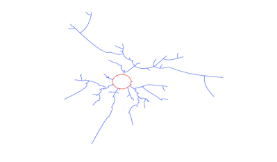
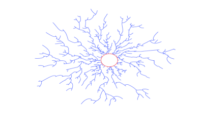
Figure 4.1. Left: compound Poisson Loewner evolution with $r=0$, $\lambda=50$ at $T=2$. Right: compound Poisson Loewner evolution with $r=0,\lambda=300$ at $T=2$.

We can now make our previous remarks more precise. We let $d_{H}$ denote the Hausdorff metric on compact subsets of $\mathbb{C}$.

Proposition 4.1.

Fix $T,\,\lambda>0$. Let $K_{T}^{r}$ be the hull obtained by evaluating the solution to (2.3) with (4.2) as driving function at $t=T$. Then, as $r\to 1$, the law of $K_{T}^{r}$ converges weakly with respect to $d_{H}$ to a point mass at the set $\overline{\mathbb{D}}\cup[1,1+\delta]$, where

$$\delta=2e^{2T}(1+\sqrt{1-e^{-2T}})-2.$$

Proof.

The discussion above shows that the driving process $\xi_{r}$ converges in law to the function identically $1$, when $r\to 1$. Hence we may couple the sequence $\xi_{r}$ so that $\xi_{r}\to 1$ a.s., see [Dur95, Page 85].

Note that the capacity of $K_{T}^{r}$ is $e^{T}$ for all $r$. Put $\Gamma_{T}^{r}=K_{T}^{r}\setminus\overline{\mathbb{D}}$. By Lemma 4.2 below, $\Gamma_{T}^{r}$ is contained in an arbitrarily narrow cone with apex at $0$ and with the point $1$ on its bisector. By the distortion estimates, we have

$$e^{T}\leq\operatorname{diam}(K_{T}^{r})\leq 4e^{T}.$$

We conclude that the Hausdorff limit of $\Gamma_{T}^{r}$ is $(1,1+\delta]$ for some $\delta$. Note that the limiting function $f_{T}:\Delta\to\Delta\setminus[1,1+\delta]$ has expansion $e^{T}z+\cdots$ at infinity. This together with the explicit formula for $f_{T}$ yields the stated expression for $\delta$. ∎

The following is the radial version of Lemma 2.1 from [CR07].

Lemma 4.2.

Let $\xi(t)$ be the driving function in (2.3). Let $\theta_{1}<\theta_{2}$ where $\theta_{j}\in[-\pi,\pi),\,j=1,2,$ and suppose that $\arg\xi(t)\in[\theta_{1},\theta_{2}]$ for $0\leq t\leq T$. Then

$$K_{T}\setminus\overline{\mathbb{D}}\subset\{re^{i\theta}:\theta_{1}\leq\theta\leq\theta_{2},\,r\geq 0\}.$$

We shall now drop the assumption that $\lambda$ be kept fixed and consider the case when $\lambda=\lambda(r)=1/(1-r)$. We write $\xi_{r}=\exp(iY_{r}(t))$ for the corresponding unimodular driving process. In this case the Fourier coefficients are

(4.6) $$a_{Y_{r}(t)}(n)=\exp\left[t\frac{r^{|n|}-1}{1-r}\right],\quad n\neq 0.$$

Letting $r\to 1$ in (4.6), we observe that $(r^{|n|}-1)/(1-r)\to-|n|$. Hence

$$\lim_{r\to 1}a_{Y_{r}(t)}(n)=\exp\left[-t|n|\right],\quad n\neq 0,$$

and these are the Fourier coefficients of a Cauchy process on $\mathbb{T}$. By appealing to Corollary 3.2 and Lemma 2.3 we have proved

Proposition 4.3.

Fix $T>0$. For each $r<1$ let $f_{T}^{r}$ denote the solution to (2.3) at $t=T$ with $\xi_{r}=\xi_{r,1/(1-r)}$ as driving process. Let $f$ denote the solution to (2.3) at $t=T$ with a unimodular Cauchy process as driving process. Then, as $r\to 1$, the law of $e^{-T}f_{T}^{r}$ converges weakly in $\Pi(\Sigma^{\prime})$ to that of $e^{-T}f_{T}$.

A systematic study of Loewner evolutions in a half-plane driven by the Cauchy process has recently been carried out by Chen and Rohde (see [CR07]).

4.2. Related models

We have also studied a related model. Instead of keeping the parameter $r$ fixed in the definition of the law of $X^{r}$, we let $r$ be a random variable on $[0,1]$ with density

$$f_{r}^{\beta}(x)=\beta x^{\beta-1}\quad\rm{for}\quad\beta>0.$$

A computation then shows that the density of the new random variable $X_{\beta}$ is given by

(4.7) $$f_{X_{\beta}}(\theta)=\frac{1}{2\pi}+\frac{\beta}{\pi}\sum_{n=1}^{\infty}\frac{\cos n\theta}{n+\beta},\quad\theta\in[-\pi,\pi].$$

We then define the compound Poisson process $Y_{\beta,\lambda}$ as before, and use $\xi_{\beta,\lambda}=\exp(iY_{\beta,\lambda})$ as driving function. The Fourier coefficients of the process are

$$a_{Y(t)}(n)=\exp\left\{-\lambda t\left(\frac{n}{\beta+n}\right)\right\}.$$

The qualitative behavior of this model is similar, and all our results go through with minor modifications: $\beta$ is a localizing parameter, and we obtain the Cauchy process in the limit $\beta=\lambda$, $\beta\rightarrow\infty$.

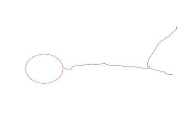
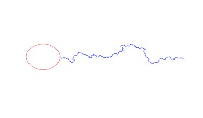
Figure 4.2. Left: compound Poisson Loewner evolution with $r=\beta=\lambda=1000$ at $T=1$. Right: compound Poisson Loewner evolution with $\gamma=8\pi^{2}/\lambda$, $\lambda=4000$ at $T=1$.

We could of course exchange the Poisson kernel in the definition of the density of the jumps of the compound Poisson process in favor of some other density. For instance, we could choose $X_{\gamma}$ distributed according to the heat kernel with parameter $\gamma>0$,

$$k_{\gamma}(\theta)=\sum_{n=-\infty}^{\infty}e^{-\gamma n^{2}}e^{in\theta}.$$

In this case, there is no interpretation of the growth model in terms of harmonic measure, except if we let $\gamma\rightarrow\infty$ since we then recover our previous model with $r=0$. However, we may note the following. The Fourier coefficients of the resulting process $\xi=\exp(iY_{\gamma,\lambda})$ are

$$a_{Y(t)}(n)=\exp\{\lambda t[\exp(-n^{2}\gamma)-1]\}.$$

Taking $\lambda=c/\gamma$ and letting $\gamma\to 0$, we see that the driving process converges to Brownian motion on the unit circle. Hence, by Lemma 2.3, the laws of the conformal mappings converge weakly to the law of the $\textrm{SLE}(\kappa)$ mapping if we choose $c=4\pi^{2}\kappa$. This result is analogous to [Bau03, Proposition 2], except that Bauer considers a different space of conformal mappings.

4.3. Hausdorff dimension of the limiting rescaled hulls

We again turn our attention to the model related to the Poisson kernel, where the driving function is given by (4.2). In this section, the dependence of the hulls on the parameter $\lambda$ will be of importance and, as before, we indicate this by writing $K_{t}^{r,\lambda}$ for the hulls of the evolution. The limit

$$\tilde{K}^{r,\lambda}_{\infty}=\lim_{t\rightarrow\infty}e^{-t}K_{t}^{r,\lambda}$$

exists in the sense of Theorem 3.3, and we denote the corresponding limit measure on $\Sigma^{\prime}$ by $\mathbb{P}^{r,\lambda}_{\infty}$.

The following theorem shows that the Hausdorff dimension of the limit hulls is trivial, just as in the $\rm{HL}(0)$ case. The proof follows along the main lines of Section 5 in [RZ05]. The Hausdorff and upper box-counting dimensions of a set will be denoted by $\dim_{H}$ and $\overline{\dim}_{B}$, respectively (see [Mat95] for definitions).

Theorem 4.4.

Let $r=0$, and fix $\lambda>4$. Then

$$\dim_{H}(\partial\tilde{K}^{0,\lambda}_{\infty})=1,$$

almost surely.

Proof.

We write $K_{t}=K_{t}^{0,\lambda}$. Let $\{\tau_{k}\}_{k}$ denote the waiting times of the Poisson process $N$. We note that the $\tau_{k}$:s are independent and exponentially distributed with density $\lambda e^{-\lambda t}$. Next, we write

$$T_{n}=\sum_{k=1}^{n}\tau_{k},\quad n\geq 1.$$

We find it convenient to consider the hulls $K_{n}=K_{T_{n}}$ and their rescalings; clearly, $\tilde{K}_{n}\rightarrow\tilde{K}_{\infty}$ as $n\rightarrow\infty$. Also, we let $\mathcal{F}_{t}=\sigma(\xi(s),\,0\leq s\leq t)$ be the natural filtration and write $\mathcal{F}_{n}=\mathcal{F}_{\tau_{n}}$ for the stopped sigma algebras.

The hulls $K_{n}$ may be written inductively as the union of the unit disk and $n$ curvilinear arcs $l_{k}=K_{k}\setminus K_{k-1}$:

$$K_{n}=\overline{\mathbb{D}}\cup\bigcup_{k=1}^{n}l_{k},$$

We denote the length of each arc $l_{k}$ by $\ell_{k}$. The length of $\partial K_{n}$ is then given by

$$L_{n}=2\pi+\sum_{k=1}^{n}\ell_{k}.$$

Similarily, the length of $\partial\tilde{K}_{n}$ is

$$\tilde{L}_{n}=e^{-T_{n}}\left(2\pi+\sum_{k=1}^{n}\ell_{k}\right).$$

Our strategy is to show that $\tilde{L}_{\infty}$ is finite almost surely, and this will imply the desired conclusion. To do this we prove a uniform bound on the expected lengths $\mathbb{E}[\tilde{L}_{n}]$ of the hulls $\tilde{K}_{n}$.

We note that

$$\mathbb{E}[\tilde{L}_{n}] =2\pi\mathbb{E}[e^{-T_{n}}]+\sum_{k=1}^{n}\mathbb{E}[e^{-T_{n}}\ell_{k}]$$

(4.8) $$\leq 2\pi(\mathbb{E}[e^{-2T_{n}}])^{\frac{1}{2}}+\sum_{k=1}^{n}(\mathbb{E}[e^{-2T_{n}}\ell_{k}^{2}])^{\frac{1}{2}},$$

and thus, it suffices to estimate $\mathbb{E}[e^{-2T_{n}}\ell_{k}^{2}]$ for $k=1,\ldots,n$.

Let $f_{k-1}:\Delta\rightarrow\mathbb{C}\setminus K_{k-1}$ denote the solution at time $T_{k-1}$ to (2.6) with the compound Poisson driving function $\xi$. The length of the $k^{th}$ added arc is given by the random variable

$$\ell_{k}=\int_{1}^{1+\delta_{k}}|f^{\prime}_{k-1}(re^{i\theta})|dr,$$

where $\theta$ is chosen uniformly. By the Cauchy-Schwarz inequality,

$$\ell_{k}^{2}\leq\delta_{k}\int_{1}^{1+\delta_{k}}|f^{\prime}_{k-1}(re^{i\theta})|^{2}dr.$$

Since $\theta$ is uniformly distributed, an estimate of $\mathbb{E}[e^{-2T_{n}}\ell_{k}^{2}]$ requires that we estimate the integral

(4.9) $$\frac{1}{2\pi}\int_{-\pi}^{\pi}\int_{1}^{1+\delta_{k}}|f^{\prime}_{k-1}(re^{i\theta})|^{2}drd\theta.$$

We note that $f_{k-1}(z)=e^{T_{k-1}}z+\cdots$, and apply Lemma 4.6 below to obtain

$$\frac{1}{2\pi}\int_{-\pi}^{\pi}\int_{1}^{1+\delta_{k}}|f^{\prime}_{k-1}(re^{i\theta})|^{2}drd\theta\leq Ce^{2T_{k-1}}(1+\delta_{k})^{2},$$

where $C<\infty$ is a constant that does not depend on $k$. Hence,

(4.10) $$\mathbb{E}[e^{-2\tau_{k}}\ell_{k}^{2}|\mathcal{F}_{k-1}]\leq Ce^{2T_{k-1}}\mathbb{E}[e^{-2\tau_{k}}\delta_{k}\,(1+\delta_{k})^{2}]$$

holds almost surely. Using (4.10) and properties of conditional expectation and independence, we obtain

(4.11) $$\mathbb{E}[e^{-2T_{n}}\ell_{k}^{2}] =\mathbb{E}[e^{-2(\tau_{k+1}+\cdots+\tau_{n})}]\,\mathbb{E}[e^{-2T_{k}}\ell_{k}^{2}]$$

$$=(\mathbb{E}[e^{-2\tau}])^{n-k}\,\mathbb{E}\left[\mathbb{E}[e^{-2T_{k}}\ell_{k}^{2}|\mathcal{F}_{k-1}]\right]$$

$$=(\mathbb{E}[e^{-2\tau}])^{n-k}\,\mathbb{E}\left[e^{-2T_{k-1}}\mathbb{E}[e^{-2\tau_{k}}\ell_{k}^{2}|\mathcal{F}_{k-1}]\right]$$

$$\leq C\cdot(\mathbb{E}[e^{-2\tau}])^{n-k}\,\mathbb{E}[e^{-2\tau_{k}}\delta_{k}\,(1+\delta_{k})^{2}]$$

A computation shows that $\mathbb{E}[e^{-2\tau_{k}}]=\lambda/(\lambda+2)$ and in view of (4.3), we have $\delta_{k}<4e^{2\tau_{k}}$. Hence $\mathbb{E}[e^{-2\tau_{k}}\delta_{k}\,(1+\delta_{k})^{2}]<\infty$ because of our assumption $\lambda>4$. This leads to the estimate

$$\mathbb{E}[e^{-2T_{n}}\ell_{k}^{2}]\leq C\cdot\left(\frac{\lambda}{\lambda+2}\right)^{n-k},$$

where $C=C(\lambda)$, which in turn implies that

(4.12) $$\mathbb{E}[\tilde{L}_{n}]\leq C\sum_{k=0}^{n}\left(\frac{\lambda}{\lambda+2}\right)^{\frac{n-k}{2}}\\ \leq C\sum_{k=0}^{\infty}\left(\frac{\lambda}{\lambda+2}\right)^{\frac{k}{2}}.$$

Since $\lambda/(\lambda+2)<1$, the geometric series on the right-hand side converges, and we conclude that $\mathbb{E}[\tilde{L}_{n}]$ is bounded by a constant that depends on $\lambda$ but not on $n$, which in turn implies that

(4.13) $$\mathbb{E}[\tilde{L}_{\infty}]\leq C$$

for some constant $C=C(\lambda)<\infty$.

Let $N(\delta,\partial\tilde{K}_{\infty})$ denote the minimal number of disks of radius $\delta$ needed to cover $\partial\tilde{K}_{\infty}$. There exists a constant $C<\infty$ independent of $\delta$ such that, almost surely,

$$N(\delta,\partial\tilde{K}_{\infty})\leq C\tilde{L}_{\infty}/\delta<\infty.$$

Hence, we have $\dim_{H}(\partial\tilde{K}_{\infty})\leq\overline{\dim}_{B}(\partial\tilde{K}_{\infty})\leq 1$, and the proof is complete. ∎

Corollary 4.5.

Fix $r<1$ and $\lambda>4$. Then

$$\dim_{H}(\partial\tilde{K}^{r,\lambda}_{\infty})=1,$$

almost surely.

Proof.

It is enough to note that the density of $X^{r}$ is square integrable when $r\neq 0$, and to use this fact together with the Cauchy-Schwarz inequality in (4.8). From there, we proceed as in the previous proof. ∎

Lemma 4.6.

For $f\in\Sigma^{\prime}$ and $\delta>0$, we have

$$\frac{1}{2\pi}\int_{-\pi}^{\pi}\int_{1}^{1+\delta}|f^{\prime}(re^{i\theta})|^{2}drd\theta\leq C(1+\delta)^{2},$$

where $C<\infty$ is a universal constant.

Proof.

We use the standard technique of inversion to obtain a function $F(\zeta)=1/f(1/\zeta)$, $\zeta\in\mathbb{D}$, belonging to the class $\mathcal{S}$ of univalent functions in the unit disk. A computation shows that $f^{\prime}(z)=F^{\prime}(1/z)/(z^{2}(F(1/z))^{2})$. We plug this into the integral and change variables to obtain

$$\frac{1}{2\pi}\int_{-\pi}^{\pi}\int_{1}^{1+\delta}|f^{\prime}(re^{i\theta})|^{2}drd\theta=\frac{1}{2\pi}\int_{-\pi}^{\pi}\int_{(1+\delta)^{-1}}^{1}\frac{|F^{\prime}(\rho e^{i\eta})|^{2}}{|F(\rho e^{i\eta})|^{4}}\rho^{2}d\rho d\eta.$$

The integral on the right-hand side is bounded by

$$\frac{1}{2}\int_{\mathcal{A}((1+\delta)^{-1},1)}\frac{|F^{\prime}(\rho e^{i\eta})|^{2}}{|F(\rho e^{i\eta})|^{4}}dA(w),$$

where $dA=\rho d\rho d\eta/\pi$ denotes area measure and

$$\mathcal{A}((1+\delta)^{-1},1))=\{w\in\mathbb{D}:(1+\delta)^{-1}<|w|<1\}.$$

Another change of variables yields

$$\frac{1}{2}\int_{\mathcal{A}((1+\delta)^{-1},1)}\frac{|F^{\prime}(\rho e^{i\eta})|^{2}}{|F(\rho e^{i\eta})|^{4}}dA(w)=\frac{1}{2}\int_{F\left(\mathcal{A}((1+\delta)^{-1},1)\right)}|z|^{-4}dA(z),$$

and by applying growth estimates for $\mathcal{S}$,

$$|F(z)|\geq\frac{(1+\delta)^{-1}}{(1+(1+\delta)^{-1})^{2}},\quad z\in\mathcal{A}((1+\delta)^{-1},1),$$

we find that the last integral is bounded by $C\cdot(2+\delta)^{4}/(1+\delta)^{2}<C^{\prime}\cdot(1+\delta)^{2}$. ∎

Remark 4.7.

The hypothesis $\lambda>4$ is only used to obtain an easy estimate of $\mathbb{E}[e^{-2\tau_{k}}\delta_{k}\,(1+\delta_{k})^{2}]$, and is probably not necessary for the conclusion since small $\lambda$ correspond to long arcs being added.

Remark 4.8.

We note that our result on Hausdorff dimension of the rescaled hulls is also valid for the other compound Poisson process-driven evolutions discussed in the previous subsection.

Acknowledgements

We thank Håkan Hedenmalm for suggesting the model of section 4 and for numerous useful comments and suggestions. We also thank Michael Benedicks and Boualem Djehiche for interesting discussions on the topics in this paper. We are grateful to the anonymous referee whose detailed comments helped us improve the quality of our paper.

References

- [Bau03] Robert O. Bauer. Discrete Löwner evolution. Annales de la Faculté des Sciences de Toulouse. Mathématiques, 12(4):433–451, 2003.
- [Ber96] Jean Bertoin. Lévy processes, volume 121 of Cambridge Tracts in Mathematics. Cambridge University Press, 1996.
- [Bil68] Patrick Billingsley. Convergence of Probability Measures. Wiley Series in Probability Theory and Mathematical Statistics. John Wiley and Sons, 1968.
- [CM01] Lennart Carleson and Nikolai Makarov. Aggregation in the plane and Loewner’s equation. Communications in Mathematical Physics, 216:583–607, 2001.
- [CR07] Zhen-Qing Chen and Steffen Rohde. Schramm-Loewner Equations driven by symmetric stable processes. Communications in Mathematical Physics, to appear, 2007.
- [Dur83] Peter L. Duren. Univalent functions, volume 259 of Grundlehren der mathematischen Wissenschaften. Springer-Verlag, 1983.
- [Dur95] Richard Durrett. Probability: theory and examples. Duxbury Press, Belmont, 2 ed. edition, 1995.
- [HL98] Matthew B. Hastings and Leonid S. Levitov. Laplacian growth as one-dimensional turbulence. Physica D, 116:244–252, 1998.
- [JP88] Jean Jacod and Philip Protter. Time reversal of Lévy processes. Annals of Probability, 16(2):620–641, 1988.
- [JS87] Jean Jacod and Albert N. Shiryaev. Limit theorems for stochastic processes, volume 288 of Grundlehren der mathematischen Wissenschaften. Springer-Verlag, 1987.
- [Law05] Gregory F. Lawler. Conformally Invariant Processes in the Plane. American Mathematical Society, 2005.
- [Mat95] Pertti Mattila. Geometry of sets and measures in Euclidean spaces, volume 44 of Cambridge Studies in Advanced Mathematics. Cambridge University Press, 1995.
- [RS05] Steffen Rohde and Oded Schramm. Basic properties of SLE. Annals of Mathematics (2), 161(2):879–920, 2005.
- [RZ05] Steffen Rohde and Michel Zinsmeister. Some remarks on Laplacian growth. Topology and its Applications, 152:26–43, 2005.