Applications of Nash’s Theorem to Cosmology
Talk presented at the II Indo-Brazilian Workshop on Gravitation and Cosmology,
Natal, Brazil, October 2008

Abstract

The cosmological constant problem is seen as a symptom of the ambiguity of the Riemann curvature in general relativity. The solution of that ambiguity provided by Nash’s theorem on gravitational perturbations along extra dimensions eliminate the direct comparison between the vacuum energy density and Einstein’s cosmological constant, besides being compatible with the formation of structures and the accelerated expansion of the universe.

1 The Gravitational Constant

The Gravitational constant in Newton’s gravitational law

$$\vec{F}=-ma=-G\frac{mm^{\prime}}{r^{2}}\frac{\vec{r}}{r}$$ (1)

was introduced to convert the physical dimensions $[M^{2}]/[L^{2}]$ to the dimensions of force $[M][L]/[T^{2}]$. It has the value $G=6.67\times 10^{-8}cm^{3}/gsec^{2}$, with the same value in a wide range of applications of (1). In 1914 Max Planck suggested a natural units system in which $G=c=\hbar=1$ and everything else would be measured in centimeters. For that purpose it was assumed that Newton’s equation (1) also holds at the quantum level. Under this condition, comparing the gravitational energy for $m=m^{\prime}$ with the quantum of energy for a wavelength $\lambda\approx r$, it follows that

$$E=<\vec{F}.\vec{r}>=G\frac{m^{2}}{\lambda}=\frac{\hbar c}{\lambda}$$

Together with Maxwell equations and the laws of thermodynamics, this leads to three quantities which characterize the so called Planck regime:

$$m_{P\ell}=\sqrt{\frac{\hbar c}{G}}\approx 10^{19}Gev,\;\;\;\lambda_{P\ell}=\sqrt{\frac{\hbar G}{c^{3}}}\approx 10^{-33}cm,\;\;\;t_{P\ell}=\sqrt{\frac{\hbar G}{c^{5}}}\approx 10^{-44}sec$$ (2)

Planck’s conclusion established a landmark in the development of modern physics:
”These quantities retain their natural significance as long as the law of gravitation and that of the propagation of light in a vacuum and the two principles of thermodynamics remain valid; they therefore must be found always the same, when measured by the most widely differing intelligences according to the most widely differing methods” [1].

Today, we can safely say that electrodynamics, actually all known gauge theories, and the laws of thermodynamics remain solid. However, the validity of Newton’s law at $10^{-33}$cm has not been experimentally confirmed. It has been recently shown to hold at $10^{-3}$cm, but with strong hints that it breaks down at $10^{-4}$cm [2]. It should be noted also that the constant $G$ is valid for the Newtonian space-time which has the product topology $\Sigma_{3}\times I\!\!R$, where $\Sigma_{3}$ denotes the 3-dimensional simultaneity sections, implying that the gravitational constant has the physical dimensions $[G]=[L]^{3}/[M][T]^{2}$, appropriate for 3-dimensional manifolds only.

In 1916 Newton’s gravitational law changed dramatically to general relativity, including the principles of equivalence, the general covariance and Einstein’s equations in a 4-dimensional space-time

$$R_{\mu\nu}-\frac{1}{2}Rg_{\mu\nu}=8\pi GT_{\mu\nu}$$ (3)

The Newtonian gravitational constant $G$, was retained in (3), to guarantee that the theory would reproduce the Newtonian theory in its weak field limit, without the need to change constants. However, the consequences of this are quite embarrassing: Indeed, the maintenance of $G$ in (3) originates the hierarchy problem of the fundamental interactions. While all relativistic gauge interactions are quantized at the Tev scale of energies, gravitation would be quantized only at $\approx 10^{19}Gev$, which, as we have seen, coincide with the energy level predicted by Planck for Newtonian quantum gravity, which is the weak field limit of general relativity. Furthermore, the relativistic quantum gravitational theory compatible with the physical dimensions of $G$ would be defined only in a 3-dimensional foliation of space-time, as originally conceived by Dirac [3], Arnowitt, Deser and Misner [4]. However, such foliation is not consistent with the diffeomorphism invariance of general relativity [5].

The criticism on the validity of Planck’s regime for quantum gravity is basis of the seminal paper by Nima Arkani-Hamed, Gia Dvali & Savas Dimopolous (ADD) [6] in 1998, inaugurating the brane-world program: Using the known fact that all gauge fields are defined in four dimensions, these authors proposed a solution of the hierarchy problem, assuming that the four dimensional space-time in which the known gauge interactions are confined is a submanifold embedded in a D=4+N-dimensional space, but gravitation would access the extra dimensions, with the same energy (Tev) of the gauge interactions. In the following we show how Nash’s theorem provides a mathematical support for such program, including the necessity for gravitational propagation in the extra dimensions.

2 Nash’s Theorem and Gravitational Perturbations

As far as the standard gauge theories are concerned, the 4-dimensionality of space-time is sufficient. This can be understood in more general terms as a consequence of the duality operations of the Yang-Mills equations. Defining the curvature 2-form $F=F_{\mu\nu}dx^{\mu}\wedge dx^{\nu},\;\;F_{\mu\nu}=[D_{\mu},D_{\nu}],\;\;D_{\mu}=\partial_{\mu}+A_{\mu}$ then the Yang-Mills equations are written as

$$D\wedge F=0\;\;\mbox{e}\;\;D\wedge F^{*}=4\pi j^{*}$$

where the dual of the gauge curvature 2-form $F$ is

$$F^{*}=F^{*}_{\mu\nu}dx^{\mu}\wedge dx^{\nu},\;\;F^{*}_{\mu\nu}=\epsilon_{\mu\nu\rho\sigma}F^{\rho\sigma}$$

It follows that $D\wedge F^{*}$ is a 3-form that must be isomorphic to the current 1-form $j^{*}$. This condition depends on the 4-dimensionality of the space-time [7, 8].
On the other hand, the gravitational field not being a standard gauge theory does not have such formal limitation. Therefore, it was assumed in [6] that gravity should propagate along extra dimensions. This is not al all obvious, but it has a solid mathematical justification based in the foundations of Riemannian geometry. The local curvature of a manifold is given by the Riemann tensor

$${\cal R}(U,V)W=[\nabla_{u},\nabla_{V}]W-\nabla_{[U,V]}W$$ (4)

which describes the variation of a tangent vector field $W$ when it is dragged along a four-sided contour defined by the vectors $U$ and $V$. This tensor tells about the local shape of the manifold, without comparing it to anything else that could be used as a standard of shape. This implies that (4) describe the curvature of a class of equivalence of Riemannian geometries with the same curvature, as was stated by Riemann himself [9]: ”…arbitrary cylindrical or conical surfaces [manifolds] count as equivalent to a plane…” In other words, the Riemann curvature is ambiguous in the sense that Riemannian manifolds with different local shapes have the same Riemannian curvature. This situation created some discomfort until 1873 when L. Schlaefli proposed a solution for such ambiguous situation, conjecturing that all Riemannian manifold should be embedded into a larger (Euclidean) space, the latter acting as the curvature reference [10].

General relativity does not present such curvature ambiguity because Minkowski’s space-time was set as the standard flat manifold against which all other space-time curvatures are compared. The same space-time is chosen as the ground state for the gravitational field, where particles and quantum fields are defined. This choice would be fine, were not for the experimental evidences of a small but non-zero cosmological constant. Since the presence of this constant is not compatible with the Minkowski space-time, we face a conflicting situation: Either we define particles, quantum fields and their vacua states in the Minkowski space-time using the Poincar group, or else these properties should be defined in a deSitter space-time using the deSitter group [11]. The cosmological constant and the vacuum energy density based on the Poincar symmetry cannot be present simultaneously in Einstein’s equations, without bringing up the current cosmological constant issue.

On the other hand, the embedding space suggested by Schlaefli can provide a curvature reference independently of the ground state, thus eliminating the conflict. To see how this works, consider the embedding map ${\cal X}:V_{n}\rightarrow V_{D}$, $D=n+N$ satisfying the embedding equations (Index convention: $\mu,\nu=1..n,\;a,b=n+1..D,\;A,B=1...D$)

$${{\cal X}}^{A}_{,\mu}{{\cal X}}^{B}_{,\nu}{\cal G}_{AB}={g}_{\mu\nu},\;\;{{\cal X}}^{A}_{,\mu}{\eta}^{B}_{b}{\cal G}_{AB}=0,\;\;{\eta}^{A}_{a}{\eta}^{B}_{b}{\cal G}_{AB}={g}_{ab}$$

were $\eta_{a}$ denotes $N$ vectors orthogonal to $V_{n}$. When the components of the Riemann tensor of the embedding space ${\cal R}_{ABCD}$ are written in the Gaussian frame $\{{\cal X}^{A}_{,\mu},\eta^{B}_{b}\}$, we obtain the Gauss, Codazzi and Ricci equations respectively

$${\cal R}_{ABCD}{\cal X}^{A}_{,\alpha}{\cal X}^{B}_{,\beta}{\cal X}^{C}_{,\gamma}{\cal X}^{D}_{,\delta}=R_{\alpha\beta\gamma\delta}-2g^{mn}k_{\alpha[\gamma m}k_{\delta]\beta n}$$ (5)

$${\cal R}_{ABCD}{\cal X}^{A}_{,\alpha}\eta^{B}_{b}{\cal X}^{C}_{,\gamma}{\cal X}^{D}_{,\delta}=k_{\alpha[\gamma b;\delta]}-g^{mn}A_{[\gamma mb}k_{\alpha\delta]n}$$ (6)

$${\cal R}_{ABCD}\eta^{A}_{a}\eta^{B}_{b}{\cal X}^{C}_{,\gamma}{\cal X}^{D}_{,\delta}=-2g^{mn}A_{[\gamma ma}A_{\delta]nb}-2A_{[\gamma ab;\delta]}-g^{mn}k_{[\gamma ma}k_{\delta]nb}$$ (7)

showing the components of the Riemann curvature of $V_{D}$ expressed in terms of the Riemann tensor of $V_{n}$; the extrinsic curvatures $k_{\mu\nu a}$ (one for each $\eta_{a}$) and the components of the third fundamental form $A_{\mu ab}$.

However, if the embedding space is to serve as a reference it must hold for all possible Riemannian geometries. This relevant detail is the main result of Nash’s theorem of 1956, where he introduced the concept of metric perturbations (or deformations) along the extra embedding dimensions [12]: Given the embedding of some background Riemannian geometry $V_{n}$ with metric $g_{\mu\nu}$, then we may obtain another manifold with the perturbed metric given by

$$g_{\mu\nu}\rightarrow g_{\mu\nu}+\delta g_{\mu\nu},\;\delta g_{\mu\nu}=-2k_{\mu\nu a}\delta y^{a}$$ (8)

Thus, Nash’s perturbations not only warps the manifold, but it also stretches deforms it, so that all Riemannian geometries can be generated, having the curvature of the embedding space as a reference. Nash’s theorem was soon generalized to pseudo-Riemannian spaces embedded in pseudo-Riemannian Manifolds [13].

In order to define such perturbations the embedding must be differentiable. This condition was implemented by Nash, using an smoothing operation to eliminate edges and wrinkles during the deformation. We find it easier and perhaps more fundamental to understand this condition as a consequence of the Einstein-Hilbert principle for the embedding space geometry:

$$\delta A=\delta\int{{\cal R}\sqrt{-{\cal G}}}dV=0$$ (9)

which has the meaning that the embedding space has the smoothest possible curvature. Under such condition and from equations (5)-(7), it follows that the embedding map ${\cal X}$ must also be differentiable to produce a differentiable and continuously perturbable embedded manifold. notice that in order to reproduce Einstein’s gravitation, the dynamical variables in (9) must be taken to be the components of the embedding space metric ${\cal G}_{AB}$, which are separated into the variables $g_{\mu\nu}$, $k_{\mu\nu a}$ and $A_{\mu ab}$ present in (5)-(7).

3 Cosmological Applications

The standard Friedman-Lemaitre-Robertson-Walker (FLRW) model is sufficiently simple to make it locally embedded in a 5-dimensional flat space, satisfying Nash’s differentiable conditions. Therefore, it can be taken as a background cosmology, which can be deformed along the fifth-dimension. However here we evaluate the effects of the extrinsic geometry in the FLWR background only (that is without perturbations). From (9) we obtain the 5-dimensional Einstein’s equations

$${\cal R}_{AB}-\frac{1}{2}{\cal R}{\cal G}_{AB}=8\pi G_{*}T^{*}_{AB},\;\;\;\;A,B=1..5$$

where $G_{*}$ denotes the gravitational constant, with physical dimensions appropriate for 4-dimensional hypersurfaces of the 5-dimensional space, consistent with the proposed solution of the hierarchy problem. Therefore, the value of $G$ is taken to correspond to the new Planck scale, somewhere within the Tev scale of energies [6]. $T^{*}_{AB}$ denotes the energy-momentum tensor of the known gauge fields and of ordinary matter, both confined to the 4-dimensional space-time. Since only gravitation can access the extra dimensions, general covariance cannot apply in the embedding space, but it remains valid in the 4-dimensional space-time. When the above equations are written in the Gaussian frame $\{{\cal X}^{A}_{,\mu},\eta^{B}\}$, we obtain the 4-dimensional gravitational equations (for the derivation of these equations see eg [14]),

$$R_{\mu\nu}-\frac{1}{2}Rg_{\mu\nu}+\Lambda g_{\mu\nu}+{Q}_{\mu\nu}=8\pi G_{*}T_{\mu\nu}$$ (10)

$$k_{\mu;\rho}^{\rho}\!-\!h_{,\mu}=0$$ (11)

where we have simplified the notation to $k_{\mu\nu 5}=k_{\mu\nu}$, $h=g^{\mu\nu}k_{\nu\nu}$, $K^{2}=k^{\mu\nu}k_{\mu\nu}$ and

$$Q_{\mu\nu}=-k^{\rho}{}_{\mu}k_{\rho\nu}+hk_{\mu\nu}\!\!+\!\!\frac{1}{2}(K^{2}-h^{2})g_{\mu\nu},\;\;\;Q^{\mu\nu}{}_{;\nu}=0,$$

The confinement of ordinary matter and gauge fields corresponds simply to $T_{\mu 5}=T_{55}=0$. The cosmological constant $\Lambda$ comes after the contracted Bianchi identity applied to the entire left-hand side of (10).

3.1 The Cosmological Constant Problem

Here we refer to the original cosmological constant problem described in [15]. Using the semiclassical Einstein’s equations in general relativity the quantum vacuum can be described as a perfect fluid with state equation $p_{v}=-<\rho_{v}>=$constant [16]:

$$R_{\mu\nu}-\frac{1}{2}Rg_{\mu\nu}+\Lambda g_{\mu\nu}=8\pi GT_{\mu\nu}^{m}+8\pi G<\rho_{v}>g_{\mu\nu}$$ (12)

where $T_{\mu\nu}^{m}$ stands for the classical sources. Comparing the constant terms in both sides of this equation we obtain $\Lambda/8\pi G=<\rho_{v}>$, or as it is commonly stated, the cosmological constant is the vacuum energy density. However, current observations tell that $\Lambda/8\pi G\approx 10^{-47}\;Gev^{4}$ (here, $c=1$). On the other hand, admitting that quantum field theory holds up to the Planck scale, the vacuum energy density would be $<\rho_{v}>\approx(10^{19}Gev)^{4}=10^{76}\;Gev^{4}$. This difference cannot be resolved by any known theoretical procedure in quantum field theory. Even supposing that quantum field theory holds to the Tev scale or less, the difference would be still too large to compensate. This difficulty has become to known as the cosmological constant problem.

Here we consider that the above difference is not only numerical, but it is mainly conceptual, resulting from the superposition of two incompatible ground states for the gravitational field in general relativity: The flat Minkowski ground state was chosen to be the reference of curvature, but the experimental evidences of $\Lambda/8\pi G\neq 0$ however small, point to a deSitter ground state, which is conceptually incompatible with the Minkowski’s choice. The implications being that particles and fields, their masses and spins defined by the Casimir operators of the deSitter group are different from those defined by the Poincar group, and they coincide only when $\Lambda$ vanishes.

The above numerical and conceptual conflicts can be resolved with the Schlaefli embedding conjecture as implemented by Nash, where the deSitter and Minkowski space-times may coexist. Indeed, in (10) $\Lambda/8\pi G_{*}$ is a gravitational component resulting from the gravitational equations in the embedding space. However, the vacuum energy density $<\rho_{v}>$ is a confined quantity in the space-time, regardless of the perturbations of its metric. Finally, the presence of the extrinsic curvature $k_{\mu\nu}$ the conserved quantity $Q_{\mu\nu}$ of (10), imply that those constants cannot be canceled without imposing a constraint on the extrinsic curvature, which is now part of the gravitational dynamics in the embedding space.

3.2 The Accelerated Expansion

To solve the system (10), (11) we start with the last of these equations to determine the general form of the extrinsic curvature for the FLRW metric. We find that

$$k_{ij}=\frac{b}{a^{2}}g_{ij},\;\;i,j=1,2,3,\;\;\;\;k_{44}=\frac{-1}{\dot{a}}\frac{d}{dt}\frac{b}{a}$$

where $b(t)\,(=k_{11})$ remains an arbitrary function as a consequence the confinement condition. Replacing this result in (10) we obtain the modified Friedman’s equation

$$\left(\frac{\dot{a}}{a}\right)^{2}+\frac{\kappa}{a^{2}}=\frac{4}{3}\pi G_{*}\rho+\frac{\Lambda}{3}+\frac{b^{2}}{a^{4}}$$ (13)

showing that the extrinsic curvature contributes to the accelerated expansion of the universe. To see this, as a first guess to determine $b(t)$ we have considered an analogy between the extrinsic curvature and the and x-matter (XCDM) phenomenological fluid [17]. Interpreting $Q_{\mu\nu}$ as a geometrical fluid

$$Q_{\mu\nu}=\frac{1}{8\pi G_{*}}[(p_{x}-\rho_{x})U_{\mu}U_{\nu}-\rho g_{\mu\nu}],\;\;p_{x}=\omega_{x}\rho_{x}$$

and comparing this with the geometric expression of $Q_{\mu\nu}$ for the FLRW universe, a simple equation for $b(t)$ is obtained

$$\frac{\dot{b}}{b}=\frac{1}{2}(1-3\omega_{x})\frac{\dot{a}}{a}$$

This cannot be integrated because we do not know $\omega_{x}$. However, assuming in particular that $\omega_{x}=constant=\omega_{0}$ we obtain a simple solution

$$b(t)=b_{0}(\frac{a}{a_{0}})^{\frac{1}{2}(1-3\omega_{0})}$$

Replacing in (13) we obtain the modified Friedman’s equation

$$\left(\frac{\dot{a}}{a}\right)^{2}+\frac{\kappa}{a^{2}}=\frac{4}{3}\pi G_{*}\rho+\frac{\Lambda}{3}+b_{0}^{2}\left(\frac{a}{a_{0}}\right)^{3(1+\omega_{0})}$$ (14)

where the constant $a_{0}$ corresponds to today’s radius of the universe. In particular using $G=G_{*}$ the constants $b_{0}$ and $\omega_{0}$ can be adjusted to match the accelerated expansion of the universe as compared with the XCDM phenomenological model [14].

3.3 The Dynamics of the Extrinsic Curvature

With the application of Nash’s theorem to cosmology, the extrinsic curvature assume the fundamental role of promoting the perturbations of the gravitational field. Noting that it is a symmetric rank-2 tensor field, it represents a spin-2 field in space-time, whose dynamics must be determined independently of the fluid model.

In 1954 S. Gupta noted that the Fierz-Pauli equation for a linear massless spin-2 field in Minkowski space-time has a remarkable resemblance with the linear approximation of Einstein’s equations [18]. He found that indeed such field must satisfy an equation that has the same formal structure as Einstein’s equations, defined on Minkowski’s space-time.

In order to derive Gupta’s equation for $k_{\mu\nu}$ for any curved manifold, we use an analogy with Riemannian’s geometry, keeping in mind that the geometry of the embedded space-time has been already defined by the metric $g_{\mu\nu}$.

In the case of a 5-dimensional embedding space, we replace $k_{\mu\nu}$ by a new tensor given by

$$f_{\mu\nu}=\frac{2}{K}k_{\mu\nu},\;\;\mbox{and}\;\;f^{\mu\nu}=\frac{2}{K}k^{\mu\nu}$$

so that $f^{\mu\rho}f_{\rho\nu}=\delta^{\mu}_{\nu}$. Then, the analogous to the Levi-Civita connection is

$$\Upsilon_{\mu\nu\rho}=\;\frac{1}{2}\left(f_{\rho\nu,\mu}+f_{\rho\mu,\nu}-f_{\mu\nu,\rho}\right)\;\,\;\mbox{and}\,\;\;\Upsilon_{\mu\nu}{}^{\sigma}=f^{\sigma\rho}\;\Upsilon_{\mu\nu\rho}$$

After, imposing the equivalent to ”metricity condition’ $f_{\mu\nu||\rho}=0$, we may calculate the analogous of the ”Riemann curvature” tensor

$$\mathcal{F}_{\nu\alpha\lambda\mu}=\Upsilon_{\mu\lambda\nu,\alpha}-\Upsilon_{\mu\alpha\gamma,\lambda}+\Upsilon_{\alpha\sigma\mu}\Upsilon_{\lambda\nu}^{\sigma}-\Upsilon_{\lambda\sigma\mu}\Upsilon_{\alpha\nu}^{\sigma}$$

and define Ricci and scalar tensors respectively by $\mathcal{F}_{\mu\nu}=f^{\alpha\beta}\mathcal{F}_{\mu\alpha\beta\nu}$, $\mathcal{F}=f^{\mu\nu}\mathcal{F}_{\mu\nu}$. With these definitions we arrive at Gupta’s equations for the f-field

$$\mathcal{F}_{\mu\nu}-\frac{1}{2}\mathcal{F}f_{\mu\nu}=\;\alpha_{f}\tau_{\mu\nu}$$ (15)

where $\tau_{\mu\nu}$ acts like a source field for the extrinsic curvature, with a coupling constant $\alpha_{f}$. A simple example is given by the vacuum equation $\mathcal{F}_{\mu\nu}=0$ which reproduces in particular the XCDM model, but now without any appeal to the fluid analogy [19].

3.4 Structure Formation

The formation of large structures in the early universe has been mostly attributed to gravitational perturbations produced by other than baryons sources, generally referred to as the dark matter component of the universe. In the present case, the extrinsic curvature solution of (15) should have an observable effect in space-time, independently of the perturbations. Therefore, it is possible that the theoretical power spectrum obtained from (14) coincide with the observed one. In a preliminary analysis we obtain a power spectrum which is similar to the power spectrum from the cosmic microwave background radiation obtained from the WMAP experiment.

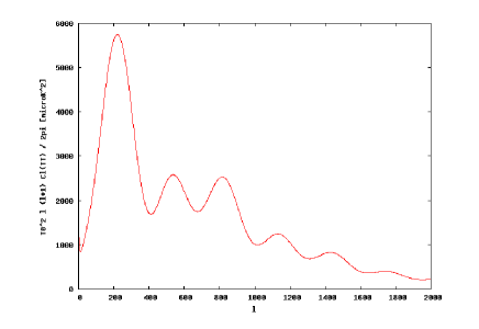
Figure 1: The NASA-CAMB theoretical power spectrum resulting from (14) calculated for $-1\leq\omega_{0}\leq-1/3$, Massive Neutrinos=1, massless neutrinos =3.04.

As we see, the third peak closely matches the observed one [20].

Concluding Remarks

The embedding of a space-time manifold into another defined by the Einstein-Hilbert principle may lead to an interesting gravitational theory, not only because its mathematical consistency provided by the Schlaefli conjecture as resolved by Nash’s theorem, but mainly because it can meet the demands of modern cosmology, with the minimum of additional assumptions.

Acknowledgements

The author wishes to thank the UFRN and the organizers of the Second Indo-Brazilian Workshop. In particular he wants to express his thanks to Edmundo Monte, Jailson Alcaniz and Abra o Capistrano for their valuable contributions to some results on the subject of this talk.

References

- [1] M. Planck. The Theory of Heat Radiation, Springer (1914). Dover edition (1959), page 175.
- [2] R. S. Decca et al: Eur. Phys. J. C51, 963, (2007). arXiv:0706.3283.
- [3] P. A. M. Dirac. Phys. Rev. 114, 924, (1959)
- [4] R. Arnowitt, S. Deser and C. Misner. The Dynamics of General Relativity. In Gravitation: An introduction to Current Research, L. Witten, Ed. John Willey & Sons, p. 227, (1962)
- [5] K. V. Kuchar. Time and Interpretations of Quantum Gravity Can. Conf. on general Relativity and relativistic Astrophys. World. Scientific (1991).
- [6] N. Arkani-Hamed, G. Dvali & S. Dimopoulos. Phys. Lett. B429, 263 (1998), Phys. Rev. Lett. 84, 586, (2000)
- [7] S. K. Donaldson. Contemporary Mathematics (AMS) 35, 201 (1984)
- [8] C. H. Taubes. Contemporary Mathematics (AMS), 35, 493 (1984)
-
[9]
B. Riemann On the Hypotheses that Lie at the Bases of Geometry (1854).
English Translation by W. K. Clifford, Nature, 8,114 (1873). - [10] L. Schlaefli, Ann. di Mat. 5, 170 (1873).
-
[11]
M. D. Maia, A. J. S. Capistrano & E. M. Monte. The Nature of the Cosmological Constant Problem.
To appear in Intl. Jour. Mod. Phys. A, (2008). - [12] J. Nash. Ann. Maths. 63, 20 (1956).
- [13] R. Greene. Mem. Amer. Math. Soc. 97, 1 (1970).
- [14] M.D. Maia , E.M. Monte, J.M.F. Maia, J.S. Alcaniz. C.Q.G. 22 1623 (2005), astro-ph/0403072.
- [15] S. Weinberg. Rev. Mod. Phys. 61, 1, (1989).
-
[16]
Ya. B. Zel’dovich & I. D. Novikov. The Structure and Evolution of the Universe,
(Chicago U. P. 1983). - [17] M. Turner & M. White. Phys.Rev. D56, 4439, (1997), arXiv:astro-ph/9701138
- [18] S. N. Gupta. Phys. Rev. 96, (6) (1954).
- [19] M. D. Maia, A. J. S. Capistrano, J. Alcaniz, E. M. Monte. Geometry of Dark Energy II. Preprint in preparation, expected to next December.
- [20] M. D. Maia, A. J. S. Capistrano & D. Muller. Perturbations of Dark Matter Gravity . Preprint available.