Homoclinic Orbits around Spinning Black Holes II:The Phase Space Portrait

Abstract

In paper I in this series, we found exact expressions for the equatorial homoclinic orbits: the separatrix between bound and plunging, whirling and not whirling. As a companion to that physical space study, in this paper we paint a phase space portrait of the homoclinic orbits that includes exact expressions for the actions and fundamental frequencies. Additionally, we develop a reduced Hamiltonian description of Kerr motion that allows us to track groups of trajectories with a single global clock. This facilitates a variational analysis, whose stability exponents and eigenvectors could potentially be useful for future studies of families of black hole orbits and their associated gravitational waveforms.

I Introduction

The transition from inspiral to plunge is a crucial landmark in the radiative evolution of a compact object falling into a supermassive black hole. A natural physical divide, the transition is also a natural conceptual divide. The inspiral can be modeled as adiabatic evolution through a sequence of Kerr geodesics Flanagan:1997sx1 ; glampedakis2002:2 ; drasco2004 ; drasco2005 ; drasco2006 ; lang2006 while the plunge is currently best modeled by numerical relativity pretorius2006 ; herrmann2007 ; campanelli2007 ; campanelli2006 ; baker2005 ; marronetti2007 ; scheel2006 . Inspiral gives way to plunge through an important family of separatrices. In paper I in this series levin2008:3 , we detailed the nature of the separatrix between bound and plunging orbits as a homoclinic orbit – an orbit in the black hole spacetime that whirls an infinite number of times as it asymptotes to an unstable circle. We found exact solutions for the family of homoclinic trajectories and depicted them as the infinite limit of a sequence of zoom-whirls levin2008:3 . As a companion to that physical space picture, we analyze the complementary phase space picture here.

As discussed at some length in paper I, formally, the homoclinic orbit lies on the intersection of the stable and unstable manifolds of a hyperbolic invariant set. In the black hole spacetime, the hyperbolic invariant set is recognized by the more familiar tag “unstable circular orbit”. To make this connection precise from the phase space perspective, we examine the variational equations – the equations governing the evolution of small displacements from the circular orbits. It is straightforward to show that the energetically bound, unstable circular orbits are hyperoblic; that is, they have an unstable eigendirection and a stable eigendirection. We then show that the stable and unstable eigendirections are tangent to the homoclinic orbit in the local neighborhood of the unstable circular orbit. In other words, two of the eigensolutions of the variational equations around bound unstable circular orbits are local representations of the homoclinic orbit. These eigensolutions capture the qualitative and quantitative features of the separatrix discussed in paper I, including the azimuthal motion levin2008:3 .

We begin by devising a reduced Hamiltonian formulation of equatorial Kerr motion that natrually admits comparisons of groups of trajectories against a single global clock. The variation of Hamilton’s equations yields stability exponents for circular orbits that could have general utility, for instance, as an estimate of inspiral or merger timescales Cornish:2001jy ; cornish2003 , or in a coarse graining of the template space around periodic orbits levin2008 . For completeness, we also find explicit expressions for the actions and the frequencies

II Kerr homoclinic orbits in phase space

Carter famously reduced the full geodesic equations of motion to four first order equations in space and time coordinates carter1968 . Despite the appeal of this accomplishment, a phase space analysis requires variation of the full equations of motion for both the coordinates and their conjugate momenta. For this reason we will not work in the first-order integrated system of equations, although we will borrow his familiar expressions. Instead, we write down a Hamiltonian formulation of Kerr geodesic motion and explicitly derive the equations of motion.

II.1 Kerr Equations of Motion

Although written out in many places, including paper I levin2008:3 , to remain self-contained we include the Kerr metric in Boyer-Lindquist coordinates and geometrized units ($G=c=1$):

$$\begin{split}ds^{2}&=-\left(1-\frac{2Mr}{\Sigma}\right)dt^{2}-\frac{4Mar\sin^{2}\theta}{\Sigma}dtd\varphi\\ &\mathrel{\phantom{=}}{}+\sin^{2}\theta\left(r^{2}+a^{2}+\frac{2Ma^{2}r\sin^{2}\theta}{\Sigma}\right)d\varphi^{2}\\ &\mathrel{\phantom{=}}{}+\frac{\Sigma}{\Delta}dr^{2}+\Sigma d\theta^{2}\end{split}\quad,$$ (1)

where $M,a$ denote the central black hole mass and spin angular momentum per unit mass, respectively, and

$$\begin{split}\Sigma&\equiv r^{2}+a^{2}\cos^{2}\theta\\ \Delta&\equiv r^{2}-2Mr+a^{2}\end{split}\quad.$$ (2)

The constants of motion along Kerr geodesics are the rest mass of the test object, energy $E$, axial angular momentum $L_{z}$, and the Carter constant $Q$ carter1968 .

In dimensionless units, the first-order geodesic equations are carter1968

$$\Sigma\dot{r} =\pm\sqrt{R}$$ (3a)

$$\Sigma\dot{\theta} =\pm\sqrt{\Theta}$$ (3b)

$$\Sigma\dot{\varphi} =\frac{a}{\Delta}\left(2rE-aL_{z}\right)+\frac{L_{z}}{\sin^{2}\theta}\qquad\quad\qquad{}^{{}^{{}^{{}^{{}^{\displaystyle,}}}}}$$ (3c)

$$\Sigma\dot{t} =\frac{(r^{2}+a^{2})^{2}E-2arL_{z}}{\Delta}-a^{2}E\sin^{2}\theta$$ (3d)

where an overdot denotes differentiation with respect to the particle’s (dimensionless) proper time $\tau$ and

$$\Theta(\theta) =Q-\cos^{2}\theta\left\{a^{2}(1-E^{2})+\frac{L_{z}^{2}}{\sin^{2}\theta}\right\}$$ (4)

$$\begin{split}R(r)&=-(1-E^{2})r^{4}+2r^{3}-\left[a^{2}(1-E^{2})+L_{z}^{2}\right]r^{2}\\ &\mathrel{\phantom{=}}{}+2(aE-L_{z})^{2}\,r-Q\Delta\qquad\qquad.\end{split}$$ (5)

The four equations  (3), though no doubt valuable in many contexts, do not lend themselves to a variational analysis. The formalism we will imploy is Hamiltonian and a phase space study requires not just the coordinates but also their conjugate momenta. Although we start from scratch with a Hamiltonian formulation of the dynamical equations, we will make use of the Eqs. (3)-(5) along the way.

As in paper I, we will restrict attention to equatorial orbits and defer non-equatorial motion to a future work. Equatorial Kerr orbits have $\theta=\pi/2$, $\dot{\theta}=0$, and $Q=0$.

II.2 Hamiltonian formulation

The Hamiltonian for a relativistic non-spinning free particle of mass $\mu$ is schmidt2002

$$H=\frac{1}{2}g^{\alpha\beta}p_{\alpha}p_{\beta}\,,$$ (6)

where the inverse metric components $g^{\alpha\beta}$ are functions of the spacetime coordinates and each $p_{\alpha}$ is both a component of the 4-momentum one-form and the canonical momentum conjugate to coordinate $q^{\alpha}$.

We want to build the Hamiltonian explicitly from Eq.  (1), and we could do so just by inserting the inverse metric and turning the crank. However, we can yield an equivalent but algebraically nicer expression for the Hamiltonian with far less effort. To begin, consider the terms in the Hamiltonian explicitly containing $p_{r}$ or $p_{\theta}$:

$$\frac{1}{2}\left(g^{rr}p_{r}^{2}+g^{\theta\theta}p_{\theta}^{2}\right)\quad.$$ (7)

Since the $r,\theta$ portion of the metric $g_{\mu\nu}$ is diagonal, that block of the inverse metric is also diagonal, with $g^{rr}=1/g_{rr}$ and $g^{\theta\theta}=1/g_{\theta\theta}$. The $p_{r},p_{\theta}$ terms in $H$ are thus

$$\frac{1}{2}\left(\frac{\Delta}{\Sigma}\right)p_{r}^{2}+\frac{1}{2}\left(\frac{1}{\Sigma}\right)p_{\theta}^{2}$$ (8)

The remaining terms in the Hamiltonian will be quadratic in the remaining momenta $p_{t}$ and $p_{\varphi}$ with coefficients that are functions only of $r$ and $\theta$ (since the metric, and thus the inverse metric, are cyclic in the $t$ and $\varphi$ coordinates). The Hamiltonian can therefore be written as

$$H(\mathbf{q},\mathbf{p})=\frac{1}{2}\left(\frac{\Delta}{\Sigma}\right)p_{r}^{2}+\frac{1}{2}\left(\frac{1}{\Sigma}\right)p_{\theta}^{2}+\frac{1}{2}F(r,\theta,p_{t},p_{\varphi})\quad,$$ (9)

where $F(r,\theta,p_{t},p_{\varphi})=F(r,\theta,E,L)$ is some expression equivalent to $g^{tt}p_{t}^{2}+2g^{t\varphi}p_{t}p_{\varphi}+g^{\varphi\varphi}p_{\varphi}^{2}$.

Notice that the $\dot{r}$ and $\dot{\theta}$ equations of (3) can be recast as

$$\begin{split}\frac{\Delta}{2\Sigma}p_{r}^{2}-\frac{R}{2\Delta\Sigma}&=0\\ \frac{1}{2\Sigma}p_{\theta}^{2}-\frac{\Theta}{2\Sigma}&=0\end{split}\quad.$$ (10)

Adding these equations and subtracting $1/2$ from both sides tells us that

$$\frac{\Delta}{2\Sigma}p_{r}^{2}+\frac{1}{2\Sigma}p_{\theta}^{2}-\frac{R}{2\Delta\Sigma}-\frac{\Theta}{2\Sigma}-\frac{1}{2}=-\frac{1}{2}\quad\quad.$$ (11)

Since $H\equiv-1/2$, the left hand side must be identical to $H$. Matching to Eq. (9), we glean that

$$F(r,\theta,E,L)=-\frac{R+\Delta\Theta}{\Delta\Sigma}-1\quad\quad,$$ (12)

so that we finally get

$$H=\frac{\Delta}{2\Sigma}p_{r}^{2}+\frac{1}{2\Sigma}p_{\theta}^{2}-\frac{R+\Delta\Theta}{2\Delta\Sigma}-\frac{1}{2}\,,$$ (13)

where $R$ and $\Theta$ are the functions in (5). Note that in dimensionless coordinates, the Hamiltonian has the same constant value $-1/2$ along any trajectory. We also used this form of the Hamiltonian in Appendix A of Ref. levin2008 .

Because all dependences on $E\equiv-p_{t}$ and $L_{z}\equiv p_{\varphi}$ are locked inside $R$ and $\Theta$ and $H$ is cyclic in $t$ and $\varphi$, Hamilton’s equations

$$\dot{q}^{\mu} =\frac{\partial H}{\partial p_{\mu}}\,,\quad \dot{p}_{\mu} =-\frac{\partial H}{\partial q^{\mu}}$$ (14)

applied to the Hamiltonian (13) yield equations of motion

$$\dot{r} =\frac{\Delta}{\Sigma}p_{r}\ ,\quad\quad \dot{p}_{r} =-\left(\frac{\Delta}{2\Sigma}\right)^{\prime}p_{r}^{2}-\left(\frac{1}{2\Sigma}\right)^{\prime}p_{\theta}^{2}+\left(\frac{R+\Delta\Theta}{2\Delta\Sigma}\right)^{\prime}$$ (15a)

$$\dot{\theta} =\frac{1}{\Sigma}p_{\theta}\ ,\quad\quad \dot{p}_{\theta} =-\left(\frac{\Delta}{2\Sigma}\right)^{\theta}p_{r}^{2}-\left(\frac{1}{2\Sigma}\right)^{\theta}p_{\theta}^{2}+\left(\frac{R+\Delta\Theta}{2\Delta\Sigma}\right)^{\theta}$$ (15b)

$$\dot{\varphi} =-\frac{1}{2\Delta\Sigma}\frac{\partial}{\partial L}\left(R+\Delta\Theta\right)\ ,\quad\quad \dot{p}_{\varphi} =0$$ (15c)

$$\dot{t} =\phantom{+}\frac{1}{2\Delta\Sigma}\frac{\partial}{\partial E}\left(R+\Delta\Theta\right)\ ,\quad\quad \dot{p}_{t} =0$$ (15d)

where the superscripts ^′ and $\theta$ denote differentiation with respect to $r$ and $\theta$, respectively. Notice, all of the Eqs. (15) are dynamically equivalent to Eqs. (3). These equations define an 8D phase space, one axis for each of the 4 coordinates $t,r,\theta,\varphi$ and their corresponding conjugate momenta, with $\tau$ parametrizing trajectories in the space. The Hamiltonian (13) derived above governs the evolution of the system in this 8-dimensional phase space.

A manifestly covariant form of Hamilton’s equations, equivalent to (14), has been used in other references to deduce important information about individual trajectories carter1968 ; schmidt2002 ; Hinderer:2008dm . We, however, want to describe how multiple trajectories evolve relative to one another to locate stable and unstable flows in phase space, and that task requires tracking evolution with respect to some global clock. In the covariant Hamiltonian picture, the time parameter $\tau$ in (14) flows differently on different trajectories and is thus not a physically viable global clock.

Coordinate time $t$ would be a good global clock, but it becomes awkward to maintain the clock as a coordinate in the 8D phase space. Furthermore, all orbits move monotonically away from the origin along the $t$ direction. Consequently, no region of finite phase volume contains any orbit in its entirety, and there are no recurrent invariant sets. The 8D space, then, is not a natural backdrop for the discussion of homoclinic orbits.

Indeed, this lack of boundedness is the hallmark of relativistic systems, in which time itself is a coordinate. Luckily, we can work in a 6D space – the phase space of spatial coordinates and their conjugate momenta – parameterized by coordinate time $t$. To do this properly, we work with a new Hamiltonian function, the energy $E$, that generates the flow parameterized by coordinate time,

$$\frac{d{q^{i}}}{dt} =\frac{\partial E}{\partial p_{i}}\,,\quad \frac{d{p_{i}}}{dt} =-\frac{\partial E}{\partial q^{i}}\quad.$$ (16)

For details of the phase space reduction formalism see Refs. Lichtenberg . It must be stressed that we treat every $E$ in the Hamiltonian (13) as an implicit function $E(\vec{q},\vec{p})$ of the spatial $q^{i}$ and $p_{i}$ and solve

$$H(\vec{q},\vec{p},E(\vec{q},\vec{p}))=-\frac{1}{2}$$ (17)

for $E$.

In other words, the spatial part of relativistic free particle motion maps to an equivalent classical problem for which coordinate time $t$ is the time parameter and whose dynamical evolution is governed by the Hamiltonian $E(\vec{q},\vec{p})$. Such a space-time splitting, which we also used in levin2008 and a fuller discussion of which we are developing in a coming work, is dynamically exact and involves no approximation. The only cost is that the accumulation of proper time $\tau$ along any trajectory (for which we will have no need in this paper anyway) must now be tracked on the side as a separate function.

To get the 6D equations of motion for the Kerr system, we could calculate $E(\vec{q},\vec{p})$ explicitly from (17) and then apply (16). Alternately, we can realize that we have to get the same result if we divide all the spatial equations in (15) by $\dot{t}$ (15d) and immediately write down

$$\frac{dr}{dt} =\frac{1}{\dot{t}}\times\frac{\Delta}{\Sigma}p_{r}\ ,\quad\quad \frac{dp_{r}}{dt} =\frac{1}{\dot{t}}\times\left\{-\left(\frac{\Delta}{2\Sigma}\right)^{\prime}p_{r}^{2}-\left(\frac{1}{2\Sigma}\right)^{\prime}p_{\theta}^{2}+\left(\frac{R+\Delta\Theta}{2\Delta\Sigma}\right)^{\prime}\right\}$$ (18a)

$$\frac{d\theta}{dt} =\frac{1}{\dot{t}}\times\frac{1}{\Sigma}p_{\theta}\ ,\quad\quad \frac{dp_{\theta}}{dt} =\frac{1}{\dot{t}}\times\left\{-\left(\frac{\Delta}{2\Sigma}\right)^{\theta}p_{r}^{2}-\left(\frac{1}{2\Sigma}\right)^{\theta}p_{\theta}^{2}+\left(\frac{R+\Delta\Theta}{2\Delta\Sigma}\right)^{\theta}\right\}$$ (18b)

$$\frac{d\varphi}{dt} =\frac{1}{\dot{t}}\times\left\{-\frac{1}{2\Delta\Sigma}\frac{\partial}{\partial L}\left(R+\Delta\Theta\right)\right\}\ ,\quad\quad \frac{dp_{\varphi}}{dt} =0$$ (18c)

with the caveat that, when we calculate derivatives of Eqs. (18), every instance of $E$ be treated as a function $E(\vec{q},\vec{p})$ rather than as either a phase space coordinate or a parameter.

This 6D phase space makes variational analysis straightforward: because coordinate time $t$ is both a good global clock and the time parameter for (16), the equations dictating the evolution in $t$ of small separations between trajectories at equal $t$ can be derived just by linearizing Eqs. (18). We perform that linearization now.

II.3 The variational equations

We work exclusively in the 6D phase space and introduce the following notational simplification. Because the distinction between $q$’s and $p$’s as components of vectors and one-forms, respectively, has to do with their behavior in the 4D manifold of the Kerr spacetime and not with their function in the phase space, where they are merely coordinates labeling points, we will henceforth drop the superscript/subscript distinction. Instead, we will refer to both $q^{i}$ and $p_{i}$ as components $X_{i}$ (with a subscript) of a single six-dimensional coordinate vector

$$\mathbf{X}\equiv\left(\begin{array}[]{c}r\\ p_{r}\\ \theta\\ p_{\theta}\\ \varphi\\ p_{\varphi}\end{array}\right)\quad.$$ (19)

This allows us to write Hamilton’s equations in the compact form

$$\frac{d\mathbf{X}}{dt}={\mathbf{f}}(\mathbf{X})\quad,$$ (20)

where the components of $\mathbf{f}$ can be read off Eq. (18).

Now consider an arbitrary reference trajectory $\mathbf{X}(t)$ in phase space and the vector $\mathbf{\delta X}(t)$ of small displacements from points on $\mathbf{X}(t)$ to points at the same coordinate time on neighboring phase trajectories. The first order equations of motion for $\mathbf{\delta X}(t)$ are the linearized full equations of motion (20) around $\mathbf{X}(t)$. Specifically,

$$\begin{split}\frac{d\,\mathbf{\delta X}(t)}{dt}&=\frac{\partial\mathbf{f}}{\partial\mathbf{X}}{\Bigg{\arrowvert}}_{\mathbf{X}(t)}\mathbf{\delta X}(t)\\ &\equiv\mathbf{K}(\mathbf{X}(t))\,\mathbf{\delta X}(t)\end{split}\quad,$$ (21)

or, componentwise,

$$\frac{d\,\delta X_{i}(t)}{dt} =K_{ij}(\mathbf{X}(t))\,\delta X_{j}(t)$$ (22)

$$\begin{split}K_{ij}(\mathbf{X})&\equiv\frac{\partial f_{i}}{\partial X_{j}}{\Bigg{\arrowvert}}_{\mathbf{X}}\qquad\quad,\\ &=\frac{\partial f_{i}}{\partial X_{j}}{\Bigg{\arrowvert}}_{\begin{subarray}{c}\text{fixed}\\ E\end{subarray}}+\frac{\partial E}{\partial X_{j}}\frac{\partial f_{i}}{\partial E}\end{split}$$ (23)

where the last equality stems from the caveat reagarding equations (18).

Equation (21) is a system of first-order linear ordinary differential equations whose coefficients $K_{ij}(t)$ depend implicitly on time through the solutions $\mathbf{X}(t)$ to (20). The solution to such a system can always be expressed in terms of a fundamental matrix Boyce $\mathbf{L}(t;\mathbf{X}_{0})$ that depends on the point $\mathbf{X}_{0}$ on the reference trajectory at which we define the initial displacement vector $\mathbf{\delta X}_{0}$ and that satisfies

$$\mathbf{\delta X}(t) =\mathbf{L}(t;\mathbf{X}_{0})\,\mathbf{\delta X}_{0}\quad,$$ (24)

where $\mathbf{L}(t=0;\mathbf{X}_{0})$ is the identity matrix.

The goal of variational analysis is to find $\mathbf{L}$, which we can equivalently think of as the time evolution operator for small displacements. Given the equations of motion (20), we can always calculate the matrix $\mathbf{K}$, but in general there is no corresponding analytic expression for $\mathbf{L}$. However, $\mathbf{K}$ on equatorial circular orbits is the constant matrix

$$\mathbf{K}=\frac{1}{\gamma\Sigma}\left(\begin{array}[]{cccccc}0&\Delta&0&0&0&0\\ \frac{R^{{}^{\prime\prime}}}{2\Delta}&0&0&0&0&\pm\frac{2r^{3/2}}{\gamma\Delta}\\ 0&0&0&1&0&0\\ 0&0&\frac{\Theta^{\theta\theta}}{2}&0&0&0\\ \mp\frac{2r^{3/2}}{\gamma\Delta}&0&0&0&0&\frac{r^{2}}{\gamma^{2}\Delta}\\ 0&0&0&0&0&0\end{array}\right)\quad,$$ (25)

where $R^{\prime\prime}$ and $\Theta^{\theta\theta}$ are the second derivatives with respect to their arguments of $R(r)$ and $\Theta(\theta)$, respectively, and $\gamma$ is a shorthand for

$$\left.\gamma\equiv\dot{t}(r)\right|_{r=\text{ circular \ orbit}}\quad.$$ (26)

Since $\mathbf{K}$ is constant, $\mathbf{L}$ has the form

$$\mathbf{L}(t)=e^{\mathbf{K}t}$$ (27)

and shares its eigenvectors with $\mathbf{K}$. Finding the eigensolutions of (21) is therefore tantamount to finding eigenvalues and eigenvectors of $\mathbf{K}$.

II.4 Eigensolutions of the variational equations

Figure 1: The dimensionless real-valued stability exponent $\lambda_{r}$ (measured in units of $M^{-1}$) for unstable circular orbits with $E<1$ for various spins $a$. Left: Prograde orbits. Right: Retrograde orbits.

The eigenvalues $\lambda$ of $\mathbf{K}$ are solutions to

$$\left|\mathbf{K}-\lambda\mathbf{I}\right|=0$$ (28)

and come in 3 pairs of equal and opposite eigenvalues whose magnitude we denote as

$$\lambda_{r} =\frac{1}{\gamma\Sigma}\sqrt{\frac{R^{\prime\prime}}{2}}\quad, \quad\lambda_{\theta} =\frac{1}{\gamma\Sigma}\sqrt{\frac{\Theta^{\theta\theta}}{2}}\quad, \quad\lambda_{\varphi} =0\quad.$$ (29)

(See also pretorius2006 ) The eigensolutions associated with the $\lambda_{\theta}$ and $\lambda_{\varphi}=0$ eigenvalues are extremely revealing in their own right. Presently, however, our concern is the eigensolutions associated with $\lambda_{r}$, and we defer a complete discussion of the eigenvectors of $\mathbf{K}$ to a future work.

The $\lambda_{r}$ may be real or imaginary depending on the sign of

$$\frac{R^{\prime\prime}}{2} =12r\left[1-(1-E^{2})r\right]-2\left[a^{2}(1-E^{2})+L_{z}^{2}\right]$$

$$=-\frac{r^{1/2}(r^{2}-6r\pm 8ar^{1/2}-3a^{2})}{r^{3/2}-3r^{1/2}\pm 2a}\quad\qquad{}^{{}^{{}^{{}^{{}^{\displaystyle,}}}}}$$ (30)

where we have used the $(E,L_{z})$ found in Ref. Bardeen1972 and used in paper I levin2008:3 to write $R^{\prime\prime}$ in terms of $r$ alone. The plus/minus signs indicate prograde/retrograde. On the unstable circular orbits of interest to us ($r_{\text{ibco}}<r<r_{\text{isco}}$), $R^{\prime\prime}$ is positive and $\lambda_{r}$ is real and plotted as a function of $r$ for various values of $a$ in Fig. 1.

The (unnormalized) eigenvectors

$$\mathbf{u}^{\scriptscriptstyle{(u)}}_{r} =\begin{pmatrix}\Delta\,,&\phantom{+}\sqrt{\frac{R^{\prime\prime}}{2}}\,,&0\,,&0\,,&\mp\frac{2r^{3/2}}{\gamma\sqrt{R^{\prime\prime}/2}}\,,&0\end{pmatrix}^{T}$$ (31)

$$\mathbf{u}^{\scriptscriptstyle{(s)}}_{r} =\begin{pmatrix}\Delta\,,&-\sqrt{\frac{R^{\prime\prime}}{2}}\,,&0\,,&0\,,&\pm\frac{2r^{3/2}}{\gamma\sqrt{R^{\prime\prime}/2}}\,,&0\end{pmatrix}^{T}$$ (32)

associated with $\pm\lambda_{r}$ are also real. Combining (24) and (27), each eigenvalue/eigenvector pair yields a corresponding eigensolution

$$\begin{split}\mathbf{\delta X^{\scriptscriptstyle{(u)}}_{r}}(t)&=c^{\scriptscriptstyle{(u)}}e^{+\lambda_{r}t}\mathbf{u}^{\scriptscriptstyle{(u)}}_{r}\\ \mathbf{\delta X^{\scriptscriptstyle{(s)}}_{r}}(t)&=c^{\scriptscriptstyle{(s)}}e^{-\lambda_{r}t}\mathbf{u}^{\scriptscriptstyle{(s)}}_{r}\end{split}$$ (33)

to the variational equation (21), where the constants $c^{\scriptscriptstyle{(u,s)}}$ reflect where we choose to set $t=0$.

II.5 Relation to the homoclinic orbits

We now build the case that in the neighborhood of $\mathbf{X^{\text{circ}}}(t)$, the linearized solutions $\mathbf{X^{\scriptscriptstyle{(u,s)}}}(t)$ coincide with exact homoclinic solutions $\mathbf{X^{\text{hc}}}(t)$. For simplicity, we focus first on the unstable solution in (33), which corresponds to a linearized solution

$$\mathbf{X^{\scriptscriptstyle{(u)}}}(t)=\mathbf{X^{\text{circ}}}(t)+\mathbf{\delta X^{\scriptscriptstyle{(u)}}_{r}}(t)$$ (34)

to the full equations of motion (20).

Some of the similarities between the linearized and homoclinic orbit are self-evident. The absence of $\theta$ and $p_{\theta}$ components in $\mathbf{X^{\scriptscriptstyle{(u)}}}(t)$ indicates that the orbit remains equatorial, and the identical signs on the $r$ and $p_{r}$ components reflect the fact that small displacements from the circular orbit along the eigendirection run away exponentially to larger radial positions and velocities on an e-folding timescale $\lambda_{r}^{-1}$. The absence of a $p_{\varphi}$ component in $\mathbf{\delta X^{\scriptscriptstyle{(u)}}_{r}}(t)$ indicates that the linearized orbit has the same angular momentum $L_{z}$ as $\mathbf{X^{\text{circ}}}(t)$.

Less self-evident is the fact that, like the homoclinic orbit, the linearized orbit also has the same energy $E$ as the circular orbit. To see this, note that since the Hamiltonian $E=E(\mathbf{X})$ is a function of the phase space coordinates, the energy difference $\delta E=E^{\text{circ}}-E^{\text{lin}}$ can be expanded as a power series in the components of $\mathbf{\delta X^{\scriptscriptstyle{(u)}}_{r}}$. Because the derivatives of all phase variables except $\varphi$ vanish on the circular orbit and $\delta p_{\varphi}=0$, the first order contribution to that expansion vanishes,

$$\begin{split}{\delta E}^{(1)}&=\frac{\partial H_{6D}}{\partial x^{i}}{\Bigg{\arrowvert}}_{r_{u}}\delta x^{i}+\frac{\partial H_{6D}}{\partial p_{i}}{\Bigg{\arrowvert}}_{r_{u}}\delta p_{i}\\ &=-\frac{dp_{i}}{dt}{\Bigg{\arrowvert}}_{r_{u}}\delta x^{i}+\frac{\partial x^{i}}{\partial t}{\Bigg{\arrowvert}}_{r_{u}}\delta p_{i}\\ &=\frac{d\varphi}{dt}\delta p_{\varphi}=0\end{split}\quad.$$ (35)

The second order variation in the energy becomes

$$\begin{split}{\delta E}^{(2)}&=\frac{\partial^{2}H_{6D}}{\partial x^{i}\partial x^{j}}{\Bigg{\arrowvert}}_{r_{u}}\delta x^{i}\delta x^{j}+\frac{\partial^{2}H_{6D}}{\partial p_{i}\partial p_{j}}{\Bigg{\arrowvert}}_{r_{u}}\delta p_{i}\delta p_{j}+2\frac{\partial^{2}H_{6D}}{\partial x^{i}\partial p_{j}}{\Bigg{\arrowvert}}_{r_{u}}\delta x^{i}\delta p_{j}\\ &=-\frac{\partial}{\partial x^{i}}\frac{dp_{j}}{dt}{\Bigg{\arrowvert}}_{r_{u}}\delta x^{i}\delta x^{j}+\frac{\partial}{\partial p_{i}}\frac{dx^{j}}{dt}{\Bigg{\arrowvert}}_{r_{u}}\delta p_{i}\delta p_{j}+2\frac{\partial}{\partial x^{i}}\frac{dx^{j}}{dt}{\Bigg{\arrowvert}}_{r_{u}}\delta x^{i}\delta p_{j}\\ &=-\frac{\partial}{\partial r}\frac{dp_{r}}{dt}{\Bigg{\arrowvert}}_{r_{u}}\delta r^{2}+\frac{\partial}{\partial p_{r}}\frac{dr}{dt}{\Bigg{\arrowvert}}_{r_{u}}\delta p_{r}^{2}+2\frac{\partial}{\partial r}\frac{dr}{dt}{\Bigg{\arrowvert}}_{r_{u}}\delta r\delta p_{r}\\ &=-K_{p_{r}r}{\Bigg{\arrowvert}}_{r_{u}}\delta r^{2}+K_{rp_{r}}{\Bigg{\arrowvert}}_{r_{u}}\delta p_{r}^{2}+2K_{rr}{\Bigg{\arrowvert}}_{r_{u}}\delta r\delta p_{r}\end{split}\quad.$$

Using Eq. (25) and the fact that

$$\delta p_{r}=\frac{1}{\Delta}\sqrt{\frac{R^{\prime\prime}}{2}}\delta r$$ (36)

on the eigensolution, we find that

$$\begin{split}&{\delta E}^{(2)}\\ &=\frac{\delta r^{2}}{\gamma\Sigma}\left(-K_{p_{r}r}{\Bigg{\arrowvert}}_{r_{u}}+K_{rp_{r}}{\Bigg{\arrowvert}}_{r_{u}}\frac{R^{\prime\prime}}{2\Delta^{2}}+2K_{rr}{\Bigg{\arrowvert}}_{r_{u}}\sqrt{\frac{R^{\prime\prime}}{2\Delta^{2}}}\right)\\ &=\frac{\delta r^{2}}{\gamma\Sigma}\left(\frac{R^{\prime\prime}}{2\Delta}+\Delta\left(\frac{1}{\Delta^{2}}\right)\frac{R^{\prime\prime}}{2}+0\right)\\ &=0\end{split}\quad.$$

A similar result holds for $\mathbf{X^{\scriptscriptstyle{(s)}}}(t)$, despite the addition of an overall minus sign in (36), since through second order $\delta E$ depends on $\delta p_{r}^{2}$. Continuing this process to higher orders is beyond the algebraic patience of the authors, but at least through second order in the variations, the linearized solutions describe orbits with the same $E$ and $L$ as the unstable circular orbit.

The $\varphi$ component of $\mathbf{\delta X^{\scriptscriptstyle{(u)}}_{r}}(t)$ merits more discussion. The ratio $\delta\varphi/\delta r$ is fixed, so that $\delta\varphi$ does not merely represent an arbitrary overall translation in $\varphi$. Instead, this component indicates how the phasing difference between the linearized orbit and the circular orbit changes as the radial separation between the two orbits grows. Notice also that since $\mathbf{\delta X^{\scriptscriptstyle{(u)}}_{r}}(t)\to 0$ as $t\to-\infty$ regardless of how $c^{\scriptscriptstyle{(u)}}$ is chosen, the linearized solution describes an orbit that is in phase with the circular orbit in the infinite past. As discussed in paper I levin2008:3 , there is a unique choice of phase for a homoclinic orbit that will synchronize it with the circular orbit in the infinite past. Apparently, the linearized eigensolution goes so far as to select the phase of the homoclinic orbit it locally approximates. The import is that the linearization captures detailed information about neighboring orbits, including phase information.

Analogously, the linearized solution

$$\mathbf{X^{\scriptscriptstyle{(s)}}}(t)=\mathbf{X^{\text{circ}}}(t)+\mathbf{\delta X^{\scriptscriptstyle{(s)}}_{r}}(t)$$ (37)

synchronizes with the circular orbit at $t=+\infty$. We can now understand the signs of the $\delta\varphi$ components of both eigenvectors. In $\mathbf{\delta X^{\scriptscriptstyle{(u)}}_{r}}(t)$ it has the opposite sign as $\delta r$ because as the displaced orbit moves to larger $r$, its $d\varphi/dt$ drops, and it lags the circular orbit with which it was synchronized at $t=-\infty$. In $\mathbf{\delta X^{\scriptscriptstyle{(s)}}_{r}}(t)$, in contrast, $\delta\varphi$ and $\delta r$ have the same sign: since the circular orbit will accumulate azimuth faster than the displaced orbit as it spirals in, it must begin ahead of the circular orbit in phase if the two are to synchronize at $t=+\infty$.

Figure 2: Projections of the eigenvector $\mathbf{u}^{\scriptscriptstyle{(u)}}_{r}$, to which the linearized separation $\mathbf{\delta X}^{\scriptscriptstyle{(u)}}$ is proportional, overlayed with the actual coordinate differences $\mathbf{X}^{\text{hc}}-\mathbf{X}^{\text{circ}}$ in the phase space. In the $\Delta\varphi$ plot, we have identified $-\pi$ at the bottom of the plot and $\pi$ at the top. The plots, intended to be schematic, are around an unstable circular orbit at $r_{u}=2.2$ for $a=0.8$.

Now, as discussed in paper I levin2008:3 , the two linearized solutions $\mathbf{X^{\scriptscriptstyle{(u)}}}(t)$ and $\mathbf{X^{\scriptscriptstyle{(s)}}}(t)$ do not coincide with the same homoclinic orbit, but rather with two homoclinic orbits that differ by a phase. Since circular orbits that differ by a phase belong to the same invariant set, we continue to refer to these as homoclinic and not heteroclinic trajectories.

II.6 Phase portraits

To make the coincidence between the linearized solutions and the homoclinic orbits manifest, we examine a phase portrait of the homoclinic orbit and the linearized solutions. Again, we use the radial coordinate $r$ along the homoclinic orbit as our global time parameter. The required expression for $p_{r}$ in terms of $r$ for the homoclinic orbit follows from Eqs.  (15a). The result is

$$p_{r}(r)=\frac{\sqrt{R(r)}}{\Delta}$$ (38)

for outbound motion and the negative of the same expression for inbound motion. Together with the exact solutions from paper I levin2008:3 , (38) generates the exact phase curves of the homoclinic orbit. Fig. 2 overlays a homoclinic orbit and the corresponding linearized orbit $\mathbf{X^{\scriptscriptstyle(u)}}$. By construction, the orbits are coincident at $t=-\infty$.

For illustration, we have plotted the case $a=0.8$ with an associated unstable circular orbit at $r_{u}=2.500536$. Since both orbits are equatorial (so that $\theta$ motion can be suppressed) and have the same $L_{z}$, a 3D orbit in $r,p_{r},\varphi$ space captures all the dynamical information, and each panel of Fig. 2 shows the projections of the two orbits into a plane. The curves in Fig. 2 are the coordinate separations between the homoclinic and circular orbits, with the various projections of the separation eigenvectors overlayed. They confirm the claim made in paper I levin2008:3 that the global stable and unstable manifolds of the circular orbits are tangent at the circular orbits to the local stable and unstable manifolds defined by the eigensolutions to the variational equations.

II.7 Action-angle variables

In an action-angle formulation schmidt2002 ; Glampedakis:2005hs ; Lichtenberg of Kerr motion, the Hamiltonian is reformulated in terms of constant momenta $J_{i}$ called actions and canonically conjugate angle variables $\psi_{i}$ that increase linearly with time at rates $\omega_{i}$. Fourier expansions of orbit functionals in terms of the fundamental frequencies $\omega_{i}$ are the basis of frequency-domain radiative evolution codes, and Ref. Hinderer:2008dm develops a description of the inspiral dynamics entirely in terms of action-angle variables. For completeness, we include exact expressions for the frequencies and actions of homoclinic orbits.

II.7.1 Fundamental frequencies

Because the equatorial Kerr system is two dimensional and integrable, every bound orbit has an associated pair of fundamental frequencies

$$\omega_{r} \equiv\frac{2\pi}{T_{r}}$$ (39a)

$$\begin{split}\omega_{\varphi}&\equiv\frac{1}{T_{r}}\int_{0}^{T_{r}}\left|\frac{d\varphi}{dt}\right|dt\\ &=\frac{2\int_{r_{p}}^{r_{a}}dr\,\left|\frac{d\varphi}{dr}\right|}{\int_{r_{p}}^{r_{a}}dr\,\frac{dt}{dr}}\end{split}\quad.$$ (39b)

Because their radial period is infinite, $\omega_{r}=0$ for homoclinic orbits. Homoclinic orbits also whirl an infinite amount as they approach their periastron $r_{u}$, so both the numerator and denominator of (39b) diverge.

However, as we show in paper I levin2008:3 , the divergences in both $T_{r}$ and the accumulated azimuth $\varphi$ can be traced to specific terms of the form

$$\left.\begin{aligned} \varphi&\to 2\frac{\Omega_{u}}{\lambda_{r}}\tanh^{-1}{\sqrt{\frac{r_{u}}{r}\frac{r_{a}-r}{r_{a}-r_{u}}}}\\ t&\to 2\frac{1}{\lambda_{r}}\tanh^{-1}{\sqrt{\frac{r_{u}}{r}\frac{r_{a}-r}{r_{a}-r_{u}}}}\end{aligned}\right.\quad\text{as $t\to T_{r}=\infty,r\to r_{u}$ .}$$ (40)

Their ratio thus converges to $\Omega_{u}\equiv d\varphi/dt(r_{u})$, the constant coordinate velocity of the circular orbit at $r_{u}$.

The azimuthal frequency for the homoclinic orbit and its associated unstable circular orbit are thus the same,

$$\begin{split}\omega_{r}^{\text{hc}}&=0\,,\\ \omega_{\varphi}^{\text{hc}}&=\left|\Omega_{u}\right|=\frac{1}{r_{u}^{3/2}+a^{2}}\end{split}\,.$$ (41)

That allows us to make a nice statement: the stable and unstable circular orbits determine the lower and upper bounds, respectively of the $\omega_{\varphi}$’s of all eccentric bound orbits with a given $L_{\text{isco}}<L_{z}<L_{\text{ibco}}$.

II.7.2 Actions

Each action $J_{i}$ of a bound orbit is defined by

$$J_{i}\equiv\oint p_{i}\,dq_{i}$$ (42)

where the integral is taken over the projection of the orbit into the $q_{i},p_{i}$ plane. Since $p_{\varphi}=L_{z}$ is constant, $J_{\varphi}=2\pi L_{z}$ for any orbit. The radial action $J_{r}$ is the area enclosed by closed $(r,p_{r})$ curves like that of Fig. 2,

$$J_{r}\equiv\oint p_{r}(r)\,dr=2\int_{r_{p}}^{r_{a}}dr\quad.$$ (43)

For arbitrary orbits, (43) at best reduces to elliptic integrals, but for the homoclinic orbit, $J_{r}$ can be written as an exact function of $r_{u}$ alone. The result, derived in the Appendix, is

$$\begin{split}J_{r}^{\text{hc}}&=2\sqrt{1-E^{2}}\times\Biggl{\{}-\sqrt{r_{u}\left(r_{a}-r_{u}\right)}+2\frac{2E^{2}-1}{1-E^{2}}\tan^{-1}\sqrt{\frac{r_{a}-r_{u}}{r_{u}}}\Biggr{\}}\\ &\mathrel{\phantom{=}}+\frac{2}{\sqrt{1-a^{2}}}\Biggl{\{}\sqrt{R(r_{\scriptscriptstyle{-}})}\tanh^{-1}\sqrt{\frac{r_{\scriptscriptstyle{-}}}{r_{a}-r_{\scriptscriptstyle{-}}}\frac{r_{a}-r_{u}}{r_{u}}}-\sqrt{R(r_{\scriptscriptstyle{+}})}\tanh^{-1}\sqrt{\frac{r_{\scriptscriptstyle{+}}}{r_{a}-r_{\scriptscriptstyle{+}}}\frac{r_{a}-r_{u}}{r_{u}}}\Biggr{\}}\end{split}\quad.$$ (44)

III conclusion

Although the results of this paper are self-contained, the phase space portrait is a direct complement to the physical space portrait of paper I levin2008:3 . Both approaches identify the separatrix between bound and plunging orbits with a homoclinic trajectory that whirls an infinite number of times on asymptotic approach to a circle.

Although the intention was to detail a profile of the separatrix, the technical results of this paper could have further utility. In partcular, the whirling stages of trajectories in the vicinity of the homoclinic set might be modeled as variations around the circular orbit using the eigenvectors and eigenvalues found here. In the future, we aim to generalize this approach to capture orbits around the periodic set levin2008 and to move out of the equatorial plane levin2008:2 ; grossman2008 .

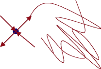
Figure 3: Schematic of a homoclinic tangle. The curve above represents the repeated intersection of a homoclinic orbit of the perturbed system with the $r,p_{r}$ phase plane. The large dot represents the intersection of a circular orbit in the perturbed system along with the eigenvectors denoting its local stable and unstable manifolds.

Another connection that should be made in a dynamical discussion of the separatirx is its role as the divide between chaotic and non-chaotic behavior. The geodesic motion of a non-spinning test particle around a Kerr black hole is known to be integrable carter1968 . There are as many constants of motion as there are canoncial momenta in this Hamiltonian system and the motion can therefore be confined to regular tori in an action-angle set of coordinates.

However, the presence of a homoclinic orbit indicates the Kerr system is vulnerable to chaos bombelli1992 ; suzuki1997 ; Suzuki:1999si ; Kiuchi:2004bv . Under perturbation, the stable and unstable manifolds that previously coincided along the homoclinic orbit (Fig. 2) can develop transverse intersections. In other words, the stable and unstable manifolds do not coincide but rather intersect, and once they intersect, they do so an infinite number of times creating a homoclinic tangle, as in Fig. 3. The homoclinic tangle is associated with a fractal set of periodic orbits and marks the locus of chaotic behavior. Chaotic behavior has in fact already been found in the Kerr system for spinning test particle motion suzuki1997 and in the case of spinning comparable mass black holes levin2000 ; levin2003 .

Chaos may be dissipated by gravitational radiation losses hartl2003b ; hartl2005 ; cornish2003:2 . However, due to the poverty of the approximation methods in the strong-field, there is no definitive resolution to the question of the survival versus extinction of chaos in astrophysical systems. If chaos does survive radiative dissipation in rapidly spinning black hole pairs, the highly non-linear character of black hole spacetimes could be evidenced by the destruction of the homoclinic orbit on transition to plunge.

Appendix A Derivation of Action of Homoclinic Orbits

The radial action of a bound non-plunging orbit is the area enclosed by its projection into the $r,p_{r}$ plane,

$$J_{r}\equiv\oint p_{r}(r)\,dr=2\int_{r_{p}}^{r_{a}}dr\frac{\sqrt{R(r)}}{\Delta}\quad,$$ (45)

where $r_{p}$ and $r_{a}$ are the periastron and apastron, respectively, and $R(r)$ is the function (5).

For a homoclinic orbit, $r_{p}$ equals $r_{u}$, the radius of the associated unstable circular orbit, and $r_{a}$ is expressible in terms of $r_{u}$ alone levin2008:3 . Additionally, $R(r)$ factors into

$$R(r)=(1-E^{2})r(r-r_{u})^{2}(r_{a}-r)\quad,$$ (46)

with $E$ the common energy of the homoclinic and unstable circular orbit. The orbit independent quantity $\Delta$ can always be factored into

$$\Delta=(r-r_{\scriptscriptstyle{+}})(r-r_{\scriptscriptstyle{-}})\quad,$$ (47)

where $r_{\scriptscriptstyle{\pm}}\equiv 1\pm\sqrt{1-a^{2}}$ are the outer and inner horizons, respectively, of the central black hole. Together, the above allows us to write the radial action (45) of a homoclinic orbit as

$$\begin{split}\frac{J_{r}^{\text{hc}}}{2\sqrt{1-E^{2}}}&=\int_{r_{u}}^{r_{a}}dr\frac{(r-r_{u})\sqrt{r(r_{a}-r)}}{(r-r_{\scriptscriptstyle{+}})(r-r_{\scriptscriptstyle{-}})}\\ &=\int_{r_{u}}^{r_{a}}dr\sqrt{\frac{r_{a}-r}{r}}\frac{r(r-r_{u})}{(r-r_{\scriptscriptstyle{+}})(r-r_{\scriptscriptstyle{-}})}\end{split}\,.$$ (48)

.

The integral in (48) can be done analytically. Under the change of variable

$$\begin{split}u=\sqrt{\frac{r}{r_{a}-r}}\,,&\mathrel{\phantom{=}}r=\frac{u^{2}}{u^{2}+1}r_{a}\\ dr\,\sqrt{\frac{r_{a}-r}{r}}&=du\,\frac{2r_{a}}{\left(1+u^{2}\right)^{2}}\end{split}\quad,$$ (49)

the factors in (48) become

$$\begin{split}r_{a}-r&=\frac{r_{a}}{1+u^{2}}\\ r-r_{u}&=\frac{u^{2}(r_{a}-r_{u})-r_{u}}{1+u^{2}}\\ r-r_{\scriptscriptstyle{+}}&=\frac{u^{2}(r_{a}-r_{\scriptscriptstyle{+}})-r_{\scriptscriptstyle{+}}}{1+u^{2}}\\ r-r_{\scriptscriptstyle{-}}&=\frac{u^{2}(r_{a}-r_{\scriptscriptstyle{-}})-r_{\scriptscriptstyle{-}}}{1+u^{2}}\end{split}$$ (50)

and (48) becomes

$$\begin{split}\!\frac{J_{r}^{\text{hc}}}{2\sqrt{1-E^{2}}}&=\frac{r_{a}-r_{u}}{\left(r_{a}-r_{\scriptscriptstyle{+}}\right)\left(r_{a}-r_{\scriptscriptstyle{-}}\right)}\times{}\\ &\mathrel{\phantom{=}}\int_{u_{u}}^{\infty}du\,\frac{2r_{a}^{2}\,u^{2}\left[u^{2}-u_{u}^{2}\right]}{\left(1+u^{2}\right)^{2}\left[u^{2}-u_{\scriptscriptstyle{+}}^{2}\right]\left[u^{2}-u_{\scriptscriptstyle{-}}^{2}\right]}\end{split}\,,$$ (51)

where

$$u_{u}^{2} \equiv\frac{r_{u}}{r_{a}-r_{u}}\,,\,\, u_{\scriptscriptstyle{+}}^{2} \equiv\frac{r_{\scriptscriptstyle{+}}}{r_{a}-r_{\scriptscriptstyle{+}}}\,,\,\, u_{\scriptscriptstyle{-}}^{2} \equiv\frac{r_{\scriptscriptstyle{-}}}{r_{a}-r_{\scriptscriptstyle{-}}}\quad.$$ (52)

The integral in (51) decomposes by partial fractions into

$$\frac{J_{r}^{\text{hc}}}{2\sqrt{1-E^{2}}}=\left(A_{1}\mathcal{I}_{1}+A_{2}\mathcal{I}_{2}+A_{3}\mathcal{I}_{3}+A_{4}\mathcal{I}_{4}\right)\bigg{\rvert}^{\infty}_{u_{u}}\quad,$$ (53)

where the coefficients $A_{i}$ are

$$\begin{split}A_{1}=r_{a}\,,&\quad A_{2}=2\left(r_{u}-2\right)\\ A_{3}=\frac{r_{\scriptscriptstyle{-}}\left(r_{u}-r_{\scriptscriptstyle{-}}\right)}{\sqrt{1-a^{2}}}\,,&\quad A_{4}=-\frac{r_{\scriptscriptstyle{+}}\left(r_{u}-r_{\scriptscriptstyle{+}}\right)}{\sqrt{1-a^{2}}}\end{split}\quad.$$ (54)

and the functions $\mathcal{I}_{i}$ are

$$\begin{split}\mathcal{I}_{1}&\equiv\int du\,\frac{2}{\left(1+u^{2}\right)^{2}}=\frac{u}{1+u^{2}}+\tan^{-1}u\end{split}$$ (55a)

$$\begin{split}\mathcal{I}_{2}&\equiv\int du\,\frac{1}{1+u^{2}}=\tan^{-1}u\end{split}$$ (55b)

$$\begin{split}\mathcal{I}_{3}&\equiv\phantom{-}\int du\,\frac{1}{u^{2}-u_{\scriptscriptstyle{-}}^{2}}=\frac{1}{2}\phantom{-}\sqrt{\frac{r_{a}-r_{\scriptscriptstyle{-}}}{r_{\scriptscriptstyle{-}}}}\ln\left[\frac{u-u_{\scriptscriptstyle{-}}}{u+u_{\scriptscriptstyle{-}}}\right]\end{split}\quad.$$ (55c)

$$\begin{split}\mathcal{I}_{4}&\equiv\int du\,\frac{1}{u^{2}-u_{\scriptscriptstyle{+}}^{2}}=\frac{1}{2}\sqrt{\frac{r_{a}-r_{\scriptscriptstyle{+}}}{r_{\scriptscriptstyle{+}}}}\ln\left[\frac{u-u_{\scriptscriptstyle{+}}}{u+u_{\scriptscriptstyle{+}}}\right]\end{split}$$ (55d)

The right hand side of (53) is easiest to evaluate in pieces. The first two terms give

$$\begin{split}\left(A_{1}\mathcal{I}_{1}\right.&+\left.A_{2}\mathcal{I}_{2}\right)\bigg{\rvert}^{\infty}_{u_{u}}=-r_{a}\frac{u_{u}}{1+u_{u}^{2}}\left(r_{a}+2r_{u}-4\right)\left(\frac{\pi}{2}-\tan^{-1}u_{u}\right)\\ &=-\sqrt{r_{u}\left(r_{a}-r_{u}\right)}+\left(r_{a}+2r_{u}-4\right)\left(\tan^{-1}\frac{1}{u_{u}}\right)\\ &=-\sqrt{r_{u}\left(r_{a}-r_{u}\right)}+2\,\frac{2E^{2}-1}{1-E^{2}}\tan^{-1}\sqrt{\frac{r_{a}-r_{u}}{r_{u}}}\end{split}\,.$$ (56)

To go from the first to the second line in (56), we have used $\tan^{-1}(u)+\tan^{-1}(1/u)=\pi/2$. To get the last line, we have used the fact that

$$r_{a}+2r_{u}=\frac{2}{1-E^{2}}$$ (57)

for homoclinic orbits, which follows from equating the cubic coefficients in equations (5) and (46).

The third term in (53) is

$$\begin{split}A_{3}\mathcal{I}_{3}\bigg{\rvert}^{\infty}_{u_{u}}&=-\frac{1}{2}\frac{\left(r_{u}-r_{\scriptscriptstyle{-}}\right)\sqrt{r_{\scriptscriptstyle{-}}\left(r_{a}-r_{\scriptscriptstyle{-}}\right)}}{\sqrt{1-a^{2}}}\ln\left[\frac{u_{u}-u_{\scriptscriptstyle{-}}}{u_{u}+u_{\scriptscriptstyle{-}}}\right]\\ &=\frac{1}{2}\frac{1}{\sqrt{1-a^{2}}}\sqrt{\frac{R(r_{\scriptscriptstyle{-}})}{1-E^{2}}}\ln\left[\frac{u_{u}+u_{\scriptscriptstyle{-}}}{u_{u}-u_{\scriptscriptstyle{-}}}\right]\\ &=\frac{1}{\sqrt{1-a^{2}}}\sqrt{\frac{R(r_{\scriptscriptstyle{-}})}{1-E^{2}}}\tanh^{-1}\frac{u_{\scriptscriptstyle{-}}}{u_{u}}\\ &=\frac{1}{\sqrt{1-a^{2}}}\sqrt{\frac{R(r_{\scriptscriptstyle{-}})}{1-E^{2}}}\tanh^{-1}\sqrt{\frac{r_{\scriptscriptstyle{-}}}{r_{a}-r_{\scriptscriptstyle{-}}}\frac{r_{a}-r_{u}}{r_{u}}}\end{split}\quad,$$ (58)

and likewise

$$\begin{split}A_{4}\mathcal{I}_{4}\bigg{\rvert}^{\infty}_{u_{u}}&=-\frac{1}{\sqrt{1-a^{2}}}\sqrt{\frac{R(r_{\scriptscriptstyle{+}})}{1-E^{2}}}\tanh^{-1}\sqrt{\frac{r_{\scriptscriptstyle{+}}}{r_{a}-r_{\scriptscriptstyle{+}}}\frac{r_{a}-r_{u}}{r_{u}}}\end{split}\quad.$$ (59)

Combining (53), (56), (58) and (59), we find that

$$\begin{split}J_{r}^{\text{hc}}&=2\sqrt{1-E^{2}}\times\Biggl{\{}-\sqrt{r_{u}\left(r_{a}-r_{u}\right)}+2\frac{2E^{2}-1}{1-E^{2}}\tan^{-1}\sqrt{\frac{r_{a}-r_{u}}{r_{u}}}\Biggr{\}}\\ &\mathrel{\phantom{=}}+\frac{2}{\sqrt{1-a^{2}}}\Biggl{\{}\sqrt{R(r_{\scriptscriptstyle{-}})}\tanh^{-1}\sqrt{\frac{r_{\scriptscriptstyle{-}}}{r_{a}-r_{\scriptscriptstyle{-}}}\frac{r_{a}-r_{u}}{r_{u}}}-\sqrt{R(r_{\scriptscriptstyle{+}})}\tanh^{-1}\sqrt{\frac{r_{\scriptscriptstyle{+}}}{r_{a}-r_{\scriptscriptstyle{+}}}\frac{r_{a}-r_{u}}{r_{u}}}\Biggr{\}}\end{split}\quad.$$ (60)

References

• (1) E. E. Flanagan and S. A. Hughes, Phys. Rev. D57, 4535 (1998).
• (2) K. Glampedakis, S. A. Hughes, and D. Kennefick, Phys. Rev. D 66, 064005 (2002).
• (3) S. Drasco and S. A. Hughes, Phys. Rev. D 69, 044015 (2004).
• (4) E. F. S Drasco and S. A. Hughes, Class. Quant. Grav. 22, 801 (2005).
• (5) S. Drasco and S. Hughes, Phys. Rev. D 73, 024027 (2006).
• (6) R. N. Lang and S. A. Hughes, Phys. Rev. D 74, 122001 (2006).
• (7) F. Pretorius, Class. Quant. Grav. 23 (2006).
• (8) F. Herrmann, I. Hinder, D. Shoemaker, P. Laguna, and R. A. Matzner, gr-qc/0701143 (2007).
• (9) M. Campanelli, C. O. Lousto, Y. Zlochower, B. Krishnan, and D. Merritt, Phys. Rev. D 75, 064030 (2007).
• (10) M. Campanelli, C. O. Lousto, P. Marronetti, and Y. Zlochower, Phys. Rev. Lett. 96, 111101 (2006).
• (11) J. G. Baker, J. Centrella, D.-I. Choi, M. Koppitz, and J. van Meter, Phys. Rev. Lett. 96, 111102 (2006).
• (12) P. Marronetti et al., Class. Quant. Grav. 24, S43 (2007).
• (13) M. A. Scheel et al., Phys. Rev. D 74, 104006 (2006).
• (14) J. Levin and G. Perez-Giz, Homoclinic Orbits around Spinning Black Holes I: Exact Solution for the Kerr Separatrix, 2008.
• (15) N. J. Cornish, Phys. Rev. D64, 084011 (2001).
• (16) N. J. Cornish and J. Levin, Class. Quant. Grav. 20, 1649 (2003).
• (17) J. Levin and G. Perez-Giz, Phys. Rev. D 77, 103005 (2008).
• (18) B. Carter, Phys. Rev. 174, 1559 (1968).
• (19) W. Schmidt, Class. Quant. Grav. 19, 2743 (2002).
• (20) T. Hinderer and E. E. Flanagan, (2008).
• (21) A. Lichtenberg and M. Liberman, Regular and Choatic Dynamics, Springer, 1992.
• (22) Boyce and DiPrima, Elementary Differential Equations and Boundary Value Problems, Wiley, 2005.
• (23) J. M. Bardeen, W. H. Press, and S. A. Teukolsky, Ap. J. 178, 347 (1972).
• (24) K. Glampedakis, Class. Quant. Grav. 22, S605 (2005).
• (25) J. Levin and R. Grossman, gr-qc/08093838 (2008).
• (26) R. Grossman and J. Levin, Dynamics of Black Hole Pairs II: Spherical Orbits and the Homoclinic Limit of Zoom-Whirl Orbits, 2008.
• (27) Bombelli and Calzetta, Class and Quant. Grav. 9, 2573 (1992).
• (28) S. Suzuki and K. ichi Maeda, Phys. Rev. D 55, 4848 (1997).
• (29) S. Suzuki and K.-i. Maeda, Phys. Rev. D61, 024005 (2000).
• (30) K. Kiuchi and K.-i. Maeda, Phys. Rev. D70, 064036 (2004).
• (31) J. Levin, Phys. Rev. Lett. 84, 3515 (2000).
• (32) J. Levin, Phys. Rev. D 67, 044013 (2003).
• (33) M. D. Hartl, Phys. Rev. D 67, 024005 (2003).
• (34) M. D. Hartl and A. Buonanno, Phys. Rev. D 71, 024027 (2005).
• (35) N. J. Cornish and J. J. Levin, Phys. Rev. D 68, 024004 (2003).