A study of the size dependence of self diffusivity across the solid-liquid transition

Manju Sharma¹ and S. Yashonath^1,2,†

¹ Solid Sate and Structural Chemistry Unit
² Center for Condensed Matter Theory
Indian Institute of Science, Bangalore, India - 560 012

Abstract

The present study investigates the effect of temperature-induced change of phase from face centred cubic solid to liquid on the size dependence of self diffusivity of solutes through detailed molecular dynamics simulations on binary mixtures consisting of a larger solvent and a smaller solute interacting via Lennard-Jones potential. The effect of change in density during the solid-liquid transition as well as in the solid and the liquid phase itself have been studied through two sets of simulations one at fixed density (NVE simulations) and another at variable density (isothermal-isobaric ensemble). A size dependent diffusivity maximum is seen in both solid and liquid phases at most densities except at low liquid densities. Two distinct regimes may be identified : linear and anomalous regimes. It is seen that the effect of solid to liquid transition is to shift the diffusivity maximum to smaller sizes of the solutes and decrease the height of the maximum. This is attributed to the predominant influence of disorder (static and dynamic) and relatively weaker influence of density. The latter shifts the diffusivity maximum towards larger solute size while the former does exactly the opposite. Interestingly, we find that lower densities lead to weaker diffusivity maximum. We report for the first time for systems with large solute-solvent interaction strength, $\epsilon_{uv}$, multiple diffusivity maximum is seen as a function of the solute size. The origin of this is not clear. A remarkable difference in the ballistic-diffusive transition is seen between solutes from the linear regime and anomalous regime. It is found that this transition is sharp for solutes from anomalous regime. Negative exponent $\alpha$ in dependence of mean square displacement on time $u^{2}(t)\ \sim\ t^{\alpha}$ is seen for linear regime solute in solid phase during ballistic-diffusive transition which is completely absent for a solute from anomalous regime. This provides interesting insight into motion of anomalous regime solutes. Apart from these, we report several properties which are different for the linear and anomalous regime solutes.

1 Introduction

We have studied in previous chapters, size dependent diffusivity in close-packed body centred cubic solid phase and also liquid phase leading to breakdown in Stokes-Einstien relationship between self diffusivity and solute diameter. Several aspects of size dependence of diffusivity has been studied in these systems. However, it is not clear how size dependent self diffusivity is altered across the solid-liquid phase transition. Several question remain unanswered that pertain to size dependent self diffusivity. Does solute diameter corresponding to diffusivity maximum shift to larger size with melting since liquids are at a lower density as compared to solids ? Can we isolate effects due to disorder and effects due to change in density ?

In this work, we report a study of size dependent diffusivity maximum across the solid-liquid transition at (a) fixed density and (b) variable density. The solid-liquid transition itself has been induced by increase in temperature rather than changes in pressure. We locate the solid-liquid transition temperature precisely for both fixed density and variable density simulations.

2 Methods

2.1 Model and intermolecular potential

Two series of runs have been made at a range of temperatures, one at fixed density referred to as FD and another in which density was allowed to vary (variable density or VD) with temperature. The system being studied is a two component system, consisting of a larger-sized solvent particles and a relatively smaller-sized solute particles. Interactions between them is via simple (6-12) Lennard-Jones potential. The solute-solvent Lennard-Jones interaction parameters have been derived from : $\sigma_{uv}$=$\sigma_{uu}$+0.7Å.[5, 9] The range of $\sigma$ and the value of $\epsilon$ chosen for solute-solute and solute-solvent and solvent-solvent interactions are listed in Table 1. The total interaction energy of the system is a sum of solvent-solvent, $U_{vv}$, solute-solvent, $U_{uv}$ and solute-solute, $U_{uu}$ interaction energy.

$$U_{tot}=U_{vv}+U_{uv}+U_{uu}$$ (1)

Initial configuration is face-centred cubic lattice of solvent with the solute occupying the octahedral voids with this lattice. The simulations are then performed at 70K. For runs at higher temperatures, the final configuration from the previous lower temperature has been taken as the starting configuration.

Table 1: Lennard-Jones interaction parameters for the solute and solvent atoms.

type of interaction	$\sigma$, Å	$\epsilon$, kJ/mol
vv	4.5	1.2
uv	1.1-2.7	4.5
uu	0.4-2.0	0.4

For variable density runs, we employed NPT ensemble at the desired temperature to obtain an estimate of the correct density. We then made runs in the microcanonical ensemble at this density. This ensures that the dynamics are computed in the microcanonical ensemble without use of NPT ensemble.

3 Computational Details

We have chosen to study the system at 70, 120, 160 and 250K which includes the solid-liquid transition. These are the temperatures for both fixed density as well as the variable density so that the different properties can be compared. The system consists of 1372 solvent and 147 solute species. The solvent and solute masses are 40 and 20amu respectively. All the simulation runs have been performed using DLPOLY.[7] The reduced density, $\rho^{*}$ for fixed density(FD) runs are 0.933 irrespective of temperature. For variable density NPT runs as well as the fixed density runs, the initial configuration for runs at all temperatures is the face-centred cubic arrangement. The initial simulation cell length of this corresponded to a reduced density of $\rho^{*}$ = 0.933 which changed to values appropriate to the new temperature. All variable density runs were made at a pressure of 0.4kbar. This pressure ensures that the system is in the liquid phase at 160K similar to the fixed density run where the solid melts at 159K. All NPT runs have been made with Berendsen method using $\tau_{T}$ and $\tau_{P}$ equal to 0.1 and 2.0ps respectively.

In all NPT runs, a timestep of 2fs for 250K and 5fs for other temperatures was used with an equilibration of 500ps and a production run of 40ps during which the average density was computed for use in NVE runs. NVE simulations were made with Verlet leapfrog algorithm with an energy conservation of total energy of better than 1 in 10^-5. An equilibration period of 1ns is followed by a production run of 2ns for computing properties. The position coordinates, velocities and forces on solutes have been accumulated every 250fs during the production run. The resulting cell dimension of the simulation cube are : for FD runs : 51.1725Å($\rho^{*}$ = 0.933), for VD runs : 48.7327Å(1.0803, VD(70K)), 49.7153Å(1.0175, VD(120K)), 52.819Å(0.8484, VD(160K)) and 56.37Å(0.6979, VD(250K)).

A few runs have been made on a smaller system of 500 solvents and 50 solutes at $\rho^{*}$ = 0.933 and 70K at different values of $\epsilon_{uv}$ (Figure 7). Here, equilibration is for 1ns while production is for 500ps.

4 Results and Discussion

The reduced densities, $\rho^{*}$ of the systems in variable density(VD) case, obtained from the simulations in isothermal-isobaric ensemble at different temperatures are reported in Table 2. The system at temperatures 70K and 120K are at 1.0803 and 1.0175 density which are higher than the density of the FD run. At 160K and 250K the densities in VD runs are 0.8484 and 0.6979, lower than the density of the fixed density(FD, $\rho^{*}$=0.933) simulation.

Table 2: The reduced densities of systems belonging to variable(VD) density case. The densities are obtained from simulations in isothermal-isobaric ensemble at 0.4kbar and temperatures, 70, 120, 160 and 250K.

T, K	$\rho^{*}$
70	1.0803
120	1.0175
160	0.8484
250	0.6979

Figure 1 shows the radial distribution(RDF) of solvent atoms at four temperatures for both VD and FD simulations. The RDF shows several well defined peaks at 70K. The positions and intensities of the peaks correspond to the face-centred cubic arrangement. Thus, the solvent is in solid phase at 70K (for both VD and FD simulations). The peaks are more sharp for the variable(VD, $\rho$*=1.0803) density system which is at higher density than the fixed (FD, $\rho$*=0.933) density system. With increase in temperature to 120K, RDF peaks are broader as compared to 70K and the system is still in the solid phase. Thus, both at 70 and 120K, the system is in the solid phase and the VD simulations yield well ordered solid as compared to FD simulations being at higher density.

At 160K the system is in liquid phase as shown in the solvent-solvent radial distribution. The RDF peaks are broader in the variable(VD, $\rho$*=0.8484) density system as the reduced density is less than the fixed(FD, $\rho$*=0.933) density system, with the VD system being more disordered. Both FD and VD systems are highly disordered liquids by 250K. The variable (VD, $\rho$*=0.6979) density system at 250K is the most disordered system among all the systems.

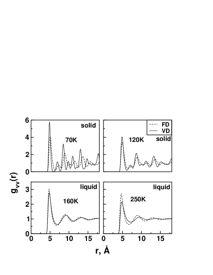
Figure 1: Solvent-solvent radial distribution plot in the solid and liquid phase for the fixed(FD) and variable(VD) density systems.

The solvent system was simulated at different temperatures to obtain the transition temperature from solid to liquid phase. Figure 2 shows the solvent-solvent radial distribution at different temperatures. The system melt at 159K as can be seen from the peaks of the radial distribution plot in the case of FD simulations. The pressure was adjusted in the case of VD simulations so as to obtain a transition temperature close to the transition temperature for the FD simulations. We found this to be the case for a pressure of 0.4kbar. Hence all simulations have been performed at 0.4kbar in case of VD simulations. The transition temperature for VD simulations is 160K.

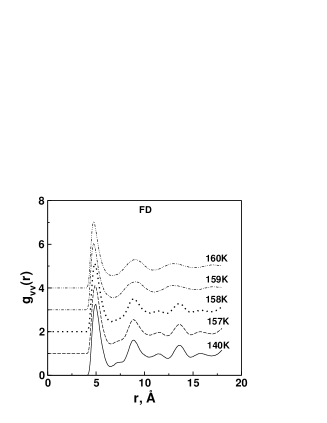
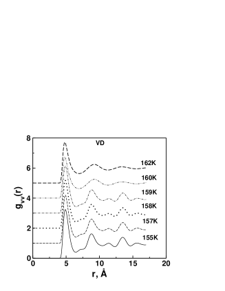
Figure 2: The transition temperatures as the system shifts from solid to liquid phase obtained from the solvent-solvent radial distribution at different temperatures for the fixed density(159K) and varied(160K) density simulations.

Further to understand the effect of change of phase and density on solvent network we have obtained the void and neck distribution of the solvent system in all the cases using Voronoi tesselation. [8] The neck is the interconnecting, usually narrower, region between any two voids. The neck size plays an important role in the size dependence of diffusion coefficient.[2, 10] Figure 3 reports both the void and the neck distribution of the solvent atoms. These have been normalized by dividing by the number of solvent particles and the number of MD steps. The neck distribution is bimodal at 70K with well defined distributions for the variable($\rho$*=1.0803) density system. For the fixed density system at $\rho$*=0.933 the distributions are less well defined as compared to VD. With increase in temperature to 120K, there is a single distribution for FD but for VD system a small shoulder still persists. The fixed(FD, $\rho$*=0.933) system density is at lower density than the variable(VD, $\rho$*=1.0175) density and thus higher disorder in FD system leads to complete merging of the second maximum with the first. At 160 and 250K, when system exists in liquid phase, the maximum in the neck distribution shifts to higher sizes. Also the width of neck distribution increases with increase in the temperature as a result of increased disorder. As we shall see, these changes have profound impact on the size-depedent diffusivity maximum. The void distribution exhibits similar changes.

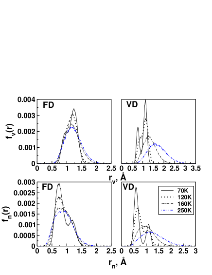
Figure 3: The normalized neck distribution of solvent atoms calculated using Voronoi tesselation as a function of phase and density.

The average neck radii, $\overline{r}_{n}$ in all the systems are calculated from the neck distribution data using the Eq. 2.

$$\overline{r}_{n}=\frac{\Sigma f_{n}(r)r}{\Sigma f_{n}(r)}$$ (2)

For the solid phases where a bimodal distribution is seen, we have obtained two average neck radii from the two distributions. The values of $\overline{r}_{n}$ for all the systems are reported in Table 3. The neck distribution and thus the average neck radii are significantly different for all the systems. In view of the previous result that the neck distribution is responsible for the size-dependent diffusivity maximum, a pertinent question is how these changes affect the diffusivity maximum as the system changes from one phase to other?

Table 3: The average neck radii obtained from Voronoi tessellation and the solute diameters for which diffusivity maximum is seen at different temperatures and densities for fixed and variable density simulations in solid and liquid phases.

T, K	phase	fixed density		variable density
		$\overline{r}_{n}$	, Å$\sigma_{uu}^{max}$, Å	$\overline{r}_{n}$, Å	$\sigma_{uu}^{max}$ Å
70	solid	0.76, 0.87	1.1, 1.5	0.60, 0.73	1.1, 1.4
120	solid	0.80	1.1	0.68, 0.79	1.1, 1.4
160	liquid	0.90	1.1	1.01	1.0
250	liquid	0.91	1.0	1.27

We have computed the mean square displacement (MSD), $u^{2}(t)$ for a range of solute diameter. These are plotted in Figure 4. Note that the msd curves are straight indicating that the statistics is good and therefore, the self diffusivity, $D$ are reliable. The self diffusivities have been obtained from the Einstein’s relationship between the mean square displacement and diffusivity. A plot of self diffusivity against solute diameter (the Lennard-Jones parameter $\sigma_{uv}$) is shown in Figure 5. Initially, for small sizes of the solute, $D$ decreases with increase in solute diameter. Subsequently, an increase in the slope is seen for intermediate sizes of the solute. This is followed by a decrease in $D$ with increase in the size of the solute at large sizes. Thus, a maximum is seen in $D$ for some intermediate size(s) of the solute. We note that previously the small solute regime where $D$ decreases with increase in solute diameter is called the linear regime (LR). The size from when $D$ increases with solute diameter and all sizes greater than this size is referred to as anomalous regime (AR).[11, 2] The maximum is seen when the diameter of the solute is comparable to the neck diameter in the distribution f($r_{n}$). Since neck diameter is not unique but a distribution of neck diameters exist, the diameter of the solute at which maximum in $D$ is seen, is influenced by the distribution f($r_{n}$).

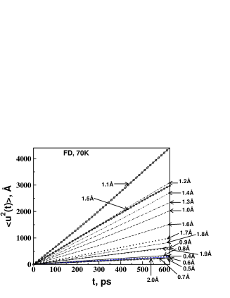
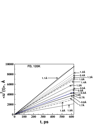
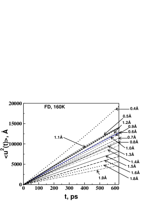
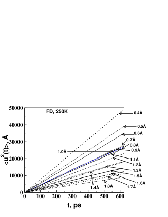
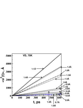
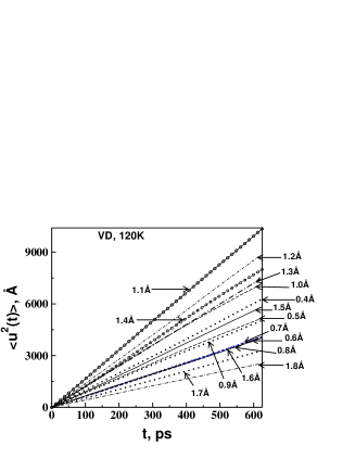
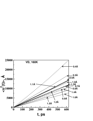
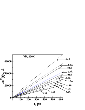
Figure 4: Time evolution of the mean square displacement of different sized solutes at four different temperatures for VD and FD simulations in solid and liquid phases.

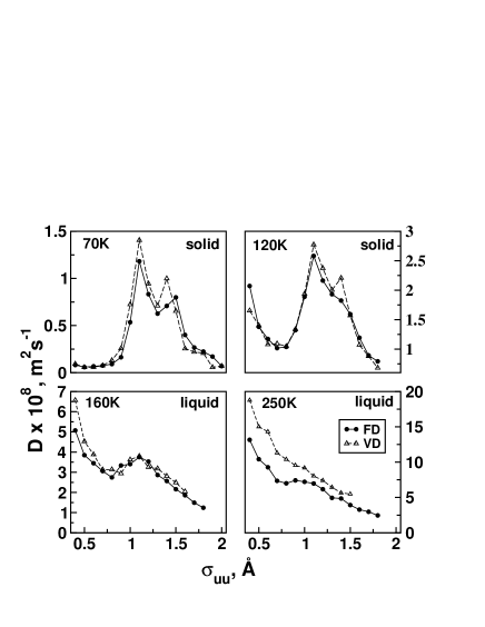
Figure 5: Impurity diffusivity as a function of size for the systems at fixed and variable densities.

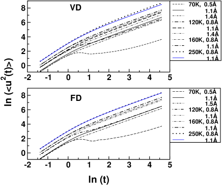
Figure 6: Logarithm of average mean square displacement as a function of logarithm of time for solutes belonging to linear(LR) and anomalous(AR) regimes at different temperatures for the fixed(FD) and varied(VD) density simulations. Note the ballistic to diffusive transition.

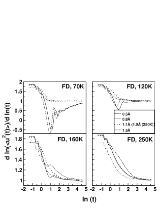
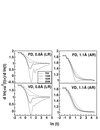
Figure 7: Derivative $d(ln\ u^{2}(t))/d(lnt)$ as a function of $ln\ t$ ($ln\ t$ = $log_{e}\ t$) for solutes belonging to linear(LR) and anomalous(AR) regimes at different temperatures for the fixed(FD) and varied(VD) density simulations. A comparison of different sizes of solutes at a given temperatures for FD and VD sets are shown in (a-b) while (c) shows same size at different temperatures for a few sizes.

In Figure 6 we show a plot of $\ln{\langle u^{2}(t)\rangle}$ against $\ln{t}$ for few solute sizes from LR and AR at different temperatures both from FD and VD simulations. The following interesting features may be seen from this. There is a transition from ballistic to diffusive regime. More importantly, the solute which are from AR (e.g. for sizes 1.1Å and 1.5Å) exhibit a rather sharp transition from ballistic to diffusive extending just from $ln\ 0$ to $ln\ 1$. The transition region is quite narrow. In contrast, solutes from LR exhibit a rather broad ballistic-diffusive transition extending over several picoseconds between $ln\ 0$ to $ln\ 4$ or higher. This is evident, for example, at 70K (VD) for a size of 0.5Å. For solutes from LR, there is effectively no change in $u^{2}(t)$ (see Figure 4) over a significant range of times in the ballistic-diffusive transition regime. Thus, for size 0.5Å  $0<\ln{t}<1$, the y-axis ($\ln{u^{2}(t)}$) changes from 1.41 to 1.62 ! This means that from 1ps to 2.71ps the mean square displacement alters from 4.1Ų to 5.1Ų. The 1.4Å sized solute, during the same interval of time has a net change in the mean square displacement of 10.1Ų (from 4.3Ų to 14.4Ų). Thus, the solute from LR, is effectively and completely localized without any mobility whatsoever during the ballistic to diffusive transition.

More insight into the nature of ballistic-diffusive transition can be obtained from the plot of derivative $d(ln\ u^{2}(t))/d(ln\ t)$ shown in Figure 7. The broad ballistic to diffusive transition for solutes from LR and the rather sharp transition for AR is evident here more clearly than in the plot of MSD. The changes in the exponent $\alpha$ in ($\langle u^{2}(t)\rangle\propto t^{\alpha}$) exhibits some unusual behaviour as is seen from the figure. First we discuss the behaviour in the face-centred cubic solid phase. $\alpha$ for solutes from AR vary between 1 and 2 at all temperatures. In contrast to this, $\alpha$ varies widely for solutes from LR, especially at low temperatures. Note that the $\alpha$ varies only in the subdiffusive regime ( 0 $<$ $\alpha$ $<$ 1) but it also becomes negative ($\alpha<$ 0) for some time at the low temperature of 70K, during the ballistic-diffusive transition period. This means that $u^{2}(t)\ \sim\ 1/\sqrt{(}t)$ for a short duration during the transition. That is, mean square displacement decreases with increase in $t$ on the average ! In the liquid phase at 160K, although the exponent $\alpha$ for the LR solute varies only between 1 and 2, a bi-exponential decay with $ln\ t$ is seen. For solute from AR, we see a single exponential decay. At higher temperature (250K), both LR and AR appear to exhibit a smooth single-exponential decay of the mean square displacement.

We propose here a tentative explanation why this is may be the case : the forces on the solute from LR exerted by the medium in which it is located is large (as we shall see below). The ballistic regime is when the solute for a short period is not experiencing the forces of the surrounding atoms (here essentially the forces due to the solvent molecules). The diffusive regime is when forces begin to alter the motion of the solute. However, the large force exerted by the solvent on a solute from LR essentially immobilizes it for a few picoseconds (during the transition period) while this is not the case for a solute from AR which continues to traverse and at the same time change to diffusive regime. This means that the LR solute is essentially trapped for an extended period just after the ballistic regime.

The diffusivity dependence on size shows certain changes with density and temperature and melting.

Solid Phase: At 70K, there are two diffusivity maxima at 1.1 and 1.5Å for fixed(FD, $\rho$*=0.933) density system whereas for the variable(VD, $\rho$*=1.0803) density system the diffusivity maxima are seen at 1.1 and 1.4Å. At a higher temperature of 120K, the diffusivity increases from 0.9Å onwards and the second diffusivity maximum disappears for the fixed density system(1.5Å). The second diffusivity maximum(1.4Å) exists for variable(VD, $\rho$*=1.0175) density system but has lower height as compared to the system at 70K(VD, $\rho$*=1.0803).

Liquid Phase: In dense fluid phase at 160K, only one diffusivity maximum is observed at 1.1Å for fixed(FD, $\rho$*=0.933) density system and variable(VD, $\rho$*=0.8484) density system as compared to two peaks in solid phase at 70K. The height of diffusity maximum in liquid phase is lower than in the solid phase. At 250K, for fixed(FD, $\rho$*=0.933) density, diffusivity maximum shifts to a lower size of 1.0Å and has a lower intensity compared to the system at 160K. In case of variable(VD, $\rho$*=0.6979) density system at 250K there is a gradual decreae in diffusivity with increase in solute size and no enhancement in diffusivity for any of the sizes is seen.

The anomalous diffusion occurs when the diameter of diffusant is comparable to the bottleneck region it passes through during diffusion.

A dimensionless parameter called levitation parameter, $\gamma$ is defined

$$\gamma=\frac{\sigma_{opt}}{\sigma_{w}}$$ (3)

where $\sigma_{opt}$ is the diffusant size at which diffusant-medium interactions are optimum and $\sigma_{w}$ is the size of the bottleneck through which the solute passes through during its passage from one void to another. In case of systems with a distribution of neck radii, the denominator is replaced by the average neck radii, $\overline{r}_{n}$. This is an approximation and does alter the value of $\gamma$ at which the maximum is seen. Note that existence of a distribution instead of a well defined single value for the bottleneck radii implies that the system is disordered. In the present study, the face-centred solid is relatively more ordered than the fluid phase but it is still disordered due to thermal motion of atoms around their equilibrium position. Typically, diffusivity maximum is seen at $\gamma\ \sim\$1 for ordered solids (without disorder due to thermal motion modeled as rigid framework) such as zeolites but at around 0.68 for dense fluids which posses dynamical disorder.[11, 2]

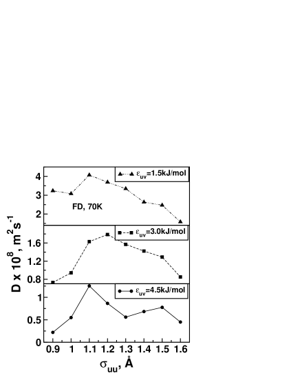
Figure 8: Impurity diffusivity as a function of size for solvent at 70K and $\rho*$=0.933 (fixed density, FD simulations) and different Lennard-Jones solute-solvent interaction parameter, $\epsilon_{uv}$.

Previous studies have shown the importance of diffusant-medium interaction. Absence of diffusant-medium dispersion interaction leads to complete absence of diffusivity maximum. Further, the ratio of $U_{uv}$/$k_{B}T$ plays an important role. When this ratio is large, then size dependent diffusivity maximum is seen but when temperature is high then diffusivity maximum is weak or absent. But, so far, only a single diffusivity maximum has been seen. However, this is the first study to report existence of double maximum. We therefore investigated this more carefully. In Figure 8 we show the results for simulations at 70K for three different values of $\epsilon_{uv}$ = 1.5, 3.0 and 4.5 kJ/mol. These have been carried out on the smaller sized system discussed earlier. We see that although a single diffusivity maximum is seen at low values of diffusant-medium interaction strength, double maximum is seen at large values. The reasons for this is not clear and requires more detailed study. It is the maximum at larger size of 1.5Å which disappears at smaller $\epsilon_{uv}$.

Changes in $D-\sigma$ behaviour as a function of melting may be understood as follows. We see two maxima at low temperatures and high densities. For example, the run at 120K (FD) which is at lower density than the VD run exhibits a single maximum. These arise from the underlying structure of the solvent as seen in terms of the void and neck distribution. We see that whenever the distribution of neck sizes $f(r_{n})$ is bimodal there are two diffusivity maxima and when $f(r_{n})$ shows a single maximum one diffusivity maximum is seen. However, there are other phases including liquid phase which show two diffusivity maxima even when $f(r_{n})$ is not bimodal [6]. This is seen whenever $\epsilon_{uv}$ is larger. Clearly, both $f(r_{n})$ and solute-solvent interactions play an important role in giving rise to diffusivity maxima.

At 70K for VD set($\rho^{*}$ = 1.0803), the bimodal distribution has maxima at 0.6 and 0.73Å leading to two maxima in $D$ at 1.1 and 1.4Å. For FD set which is at lower density ($\rho^{*}$ = 0.933), the maxima are at slightly larger size, 0.76 and 0.87Å and the maxima in $D$ are at 1.1 and 1.5Å. The reason why the maximum near 1.1Å did not shift by 0.1Å to larger size could be due to increased disorder at lower density. Effect of such disorder is to shift the maximum to smaller sizes. Thus, the two opposing effects (change in density and disorder) lead to no shift. Larger neck size which gives rise to maximum at 1.4Å is relatively less influenced by the disorder since the neck is quite large. At 120K, for VD ($\rho$*=1.0175) the $f(r_{n})$is still bimodal with $\overline{r}_{n}$= 0.68 and 0.79Åand the diffusivity maximum remains at the same position but height is decreased as compared to 70K. For FD at 120K, we see $f(r_{n})$is no more bimodal and $D-\sigma$ also exhibits a single maximum.

In the liquid phase at 160K for variable(VD, $\rho$*=0.8484) density system, diffusivity maximum is lower in intensity and occurs at 1.1Å. In this system, average neck radius is 1.01Å which is larger than the solid phase systems due to the lower density. The fixed(FD, $\rho$=0.933) density system at 160K has average neck radius of 0.90 and shows anomalous behaviour for 1.1Å. The fact that the maximum in both VD and FD occur at the same value of solute diameter in spite of the difference in the $\overline{r}_{n}$shows the predominant influence of disorder on the diffusivity maximum. At 160K, considerable disorder exists in the fluid phase and the influence of density is reduced.

At 250K, variable(VD, $\rho$*=0.6979) density system has maximum disorder and in this system solute-solvent interaction energy is not very large as compared to the kinetic energy($U_{uv}$/$k_{B}T$ $<<$ 1). Thus, the Levitation effect or the anomalous diffusion disappears and a gradual decrease in diffusivity with increase in solute size is observed. But the fixed(FD, $\rho$*=0.933) density system at 250K still has density higher than variable(VD) density system and this leads to $U_{uv}/k_{B}T$ is not as small as in the VD run. Thus, a small diffusivity maximum is seen for size 1.0Å. There is a shift of the diffusivity maximum to lower size as the system undergoes considerable decrease in density. These have been summarized in Table 3 which lists the average values of $\overline{r}_{n}$and the values of $\sigma_{uu}^{max}$ at which the diffusivity maximum is observed. Also listed are the values of $\gamma$.

We have obtained the related properties to obtain additional insight. Figure 9 displays the velocity autocorrelation(VACF) function for solutes in all the systems. Solutes corresponding to minimum diffusivity, (0.5Å for FD and VD at 70K) and 0.8Å for other systems show an oscillatory VACF with significant back scattering while solutes at diffusivity maximum decay smoothly. We attribute oscillatory behaviour for solutes from LR to an energy barrier during its passage out of the first solvent shell. Such a barrier leads to back-and-forth motion leading to back scattering. The anomalous regime solute does not experience any barrier at the first shell and consequently, VACF decays smoothly. In the solid phase, a slight back scattering is seen for the solute from AR. This could be either due to the discrete sizes of solutes (at 0.1Å interval) for which properties have been computed here. The actual diffusivity maximum might be actually somewhere in between these. Alternately, the cooperative motion in a liquid between the solute and solvent is less likely in a solid since the solvent particles in the solid phase have limited mobility.

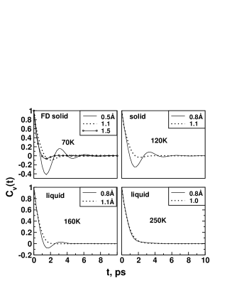
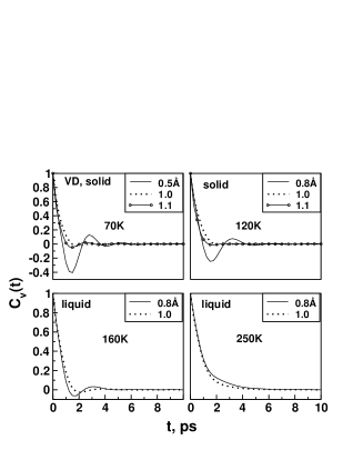
Figure 9: Velocity autocorrelation function of impurities with minimum and maximum difffusivity. The plots are reported for systems in solid and liquid phases for fixed and variable densities.

Figure 10 plots the average mean square force exerted by the surrounding atoms (predominantly solvent particles) as a function of the solute size. Solutes with maximum diffusivity experience lowest average mean square force due to the neighboring solvent atoms in all the systems. When the size of the solute is similar to the bottleneck through which it passes during diffusion, the force from a given direction is equal and opposite to that exerted by the solvent atoms diagonally opposite. The force from diagonally opposite directions mutually cancel each other and solute has a higher diffusivity. Note that the average mean square force is lowest (for all sizes of the solute) in the solid phase at 70K and with increase in temperature, there is increase in net force. This is due to increasing disorder or Brownian motion which undermines the intermolecular forces. Random forces form a significant fraction of total forces at high temperature. As the difference in the force exerted between the solute from LR and AR decreases, the diffusivity maximum also gradually disappears.

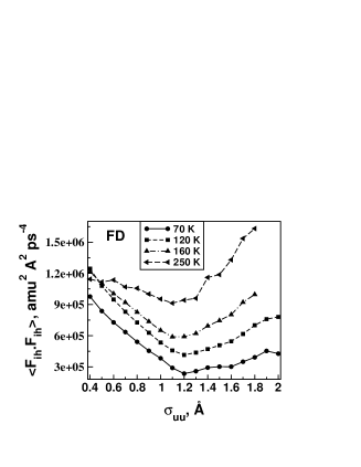
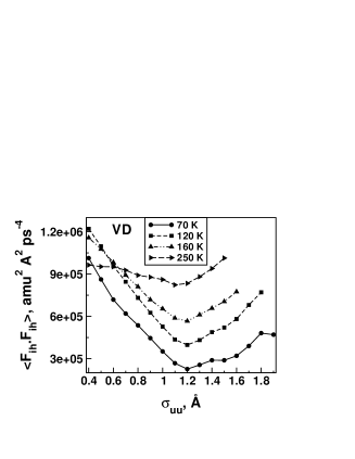
Figure 10: Average mean square force occuring on an solute due to neighbouring solvent atoms as a function of solute size for systems in different phases for fixed and variable densities.

Time evolution of the negative of logarithm of self part of the intermediate scattering functions $F_{s}(k,t)$ for solute sizes at diffusivity maximum and close to diffusivity minimum at the border between the LR and AR are shown in Figure 11. The reciprocal of the slope gives the relaxation time.[3] Note that solutes away from the diffusivity maximum exhibit two distinct slopes; at initial times the slope is large and at long times a lower slope corresponding to two relaxation times. In contrast, solute close to diffusivity maximum exhibits either a single slope or two straight lines whose slopes are almost identical to each other. The biexponential decay of $F_{s}(k,t)$ for solutes from LR suggest that the motion of the solute has two distinct regime. We suggest that the faster relaxation time of this solute corresponds to motion within the first neighbour shell of the solvent irrespective of whether the phase is solid or fluid. For solute from AR, we suggest that the solvent motion encounters no barrier past the first solvent shell and therefore there is a single relaxation time. The resulting relaxation times are listed in Table 4. With increase in temperature, the relaxation times decrease due to faster dynamics.

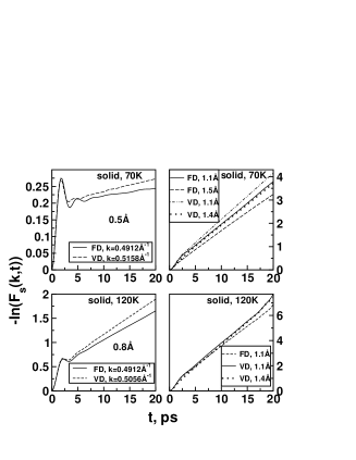
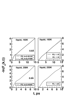
Figure 11: Logarithm of self part of the intermediate scattering function is shown for wavenumber $k$ = 2n$\pi$/L for solute sizes corresponding to minimum and maximum diffusivity in both the solid and liquid phase obtained from variable and fixed density runs. L($\rho^{*}$)=51.1725Å(0.933, FD), 48.7327Å(1.0803, VD(70K)), 49.7153Å(1.0175, VD(120K)), 52.819Å(0.8484, VD(160K)) and 56.37Å(0.6979, VD(250K)). The lines are the least square fit to the MD data.

Table 4: Relaxation times of impurities belonging to linear and anomalous regimes in different systems.

	Fixed density			Variable density
T, K	$\sigma_{uu}$,Å	k, Å-1	$\tau_{1}$, $\tau_{2}$ (ps)	$\sigma_{uu}$,Å	k, Å-1	$\tau_{1}$, $\tau_{2}$ (ps)
70	0.5	0.4912	5.68, 409.84	0.5	0.5158	5.69, 263.16
70	1.1	0.4912	5.42	1.1	0.5158	4.92
70	1.5	0.4912	6.19	1.4	0.5158	5.45
120	0.8	0.4912	2.59, 16.53	0.8	0.5056	2.50, 13.61
120	1.1	0.4912	3.06	1.1	0.5056	2.77
120				1.4	0.5056	2.74
160	0.8	0.4912	1.72, 4.25	0.8	0.4759	1.83, 4.18
160	1.1	0.4912	2.10	1.0	0.4759	1.99
250	0.8	0.4912	1.02, 1.77
250	1.0	0.4912	1.33

Full width at half maximum (fwhm) of the dynamic structure factor has been obtained by fourier transformation of the self part of the intermediate scattering function. The dependence of fwhm on $k$ gives insight into the nature of $k$-dependence of self diffusivity. In the limit of $k$ approaching 0, the hydrodynamic limit, the fwhm approaches 2D$k^{2}$ and the ratio

$$\Delta(k)=\frac{\Delta\omega(k)}{2Dk^{2}}$$ (4)

approaches unity. Figure 12 shows the wavevector dependence of self diffusivity for solutes close to to minimum and maximum diffusivity, both for solid and liquid phases. $\Delta$(k) of solute close to diffusivity maximum exhibit a monotonic decrease with $k$ both in the solid and the liquid phase. In contrast, the solute near the diffusivity minimum exhibit a minimum followed by a maximum for $k$ between 1 and 3. The minimum corresponds to slow down in diffusivity of the solute at wavenumber corresponding to first shell. Similar behaviour has been seen by Nijboer and Rahman in high density liquid argon at low temperatures [4]. Boon and Yip have noted that the minimum generally occurs for wavenumbers corresponding to first maximum in static structure factor S(k) [1]. Such a slowing down in $k$ dependent self diffusivity does not occur for solute from AR since it does not encounter any energetic barrier to go past the first solvent shell. Consequently, it has facile passage past the first shell. If the solute size is close to the maximum in diffusivity but not at the true maximum (the location of the true maximum is limited by the 0.1Å interval we have used here for the solute size) then small oscillations are seen in Figure 12.

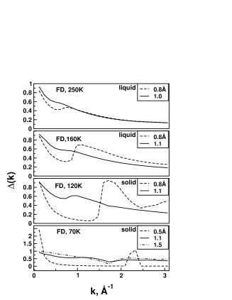
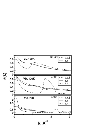
Figure 12: Wavevector dependence of impurities with minimum and maximum diffusivity in solid and liquid phase at fixed and variable density.

We have obtained the activation energies of the solute near diffusivity minimum(0.5Å and 0.8Å) and maximum(1.1Å and 1.5Å) in the solid and liquid phases for the fixed density systems. Figure 13 displays the Arrhenius plots for the solutes. Diffusivities of solutes have been computed from additional simulations at temperatures 70, 85 and 100K in the solid phase and 160, 200 and 250K in the liquid phase. The activation energy for diffusion is less for solutes with maximum diffusivity as compared to solutes located at minimum diffusivity as shown in Table 5. The difference in activation energy for minimum and maximum diffusivity is very large in the solid phase. In the liquid phase, system is dynamic and overall diffusivity of impurities of all sizes is higher than the solid phase. However, the increased influence of random forces leads to limited influence of interparticle interactions on dynamics. Thus, the difference in activation energies between the solute from LR and AR decrease. This is seen for the liquid phase for sizes 0.8 and 1.1Å. In case of solid phase, due to the predominance of solute-solvent interaction and lower kinetic energy, the difference in activation energies for solutes from LR and AR are dramatic : 4.99 kJ/mol for 0.5Å solute from LR as compared to 0.86 kJ/mol for the larger 1.5Å sized solute. This shows that the Levitation effect is more pronounced in the solid phase.

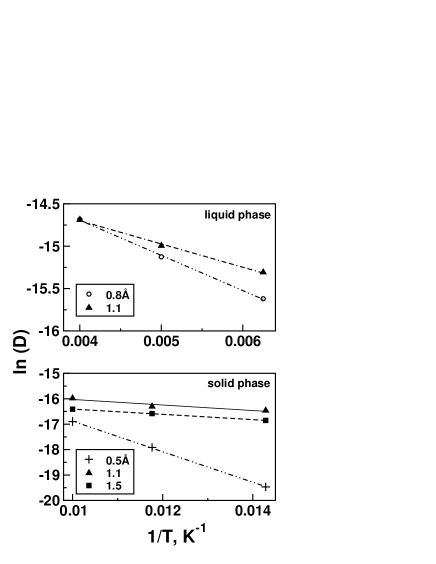
Figure 13: Arrhenius plot for impurities with diffusivity minimum and maximum in solid and liquid phase for fixed density systems.

Table 5: Activation Energy of impurities with diffusivity minimum and maximum in solid and liquid phases for fixed density systems.

$\sigma_{uu}$, Å	Phase	Regime	$E_{act}$, kJ/mol
0.5	Solid	Linear	4.9998
1.1	Solid	Anomalous	0.9070
1.5	Solid	Anomalous	0.8625
0.8	Liquid	Linear	3.4525
1.1	Liquid	Anomalous	2.2852

5 Conclusions

The main conclusions of this study are : (i) At sufficiently low density size dependent diffusivity maximum disappears altogether. (ii) Presence of dynamic disorder at high temperature does not lead to backscattering in VACF for the solute close to diffusivity maximum. (iii) Significant backscattering is seen in VACF for LR but not for AR in the solid phase. (iv) In the solid phase, the exponent $\alpha$ in $u^{2}(t)\ \sim\ t^{\alpha}$ exhibits negative exponent during ballistic to diffusive transition for the solute from LR but not from AR. (v) The solute diameter $\sigma_{uu}^{max}$ (equal to $\sigma_{uu}$ for the solute at diffusivity maximum) shifts to lower sizes at high temperature in spite of decrease in density. This is because of increase in disorder. (vi) Multiple maxima are seen in the solid phase for high $\epsilon_{uv}$. (vii) Significant shift to lower $\overline{r}_{n}$is seen across the solid-liquid transition corresponding to lower $\rho$. (viii) Correspondigly, shift is seen in $\sigma_{max}$ to smaller values.

Acknowledgement : Authors wish to thank Department of Science and Technology, New Delhi for financial support in carrying out this work. Authors also acknowledge C.S.I.R., New Delhi for a research fellowship to M.S.

References

- [1] J. P. Boon and Sidney Yip. Molecular Hydrodynamics. Dover Publications, New York, 1980.
- [2] Pradip Kr. Ghorai and S. Yashonath. The stokes-einstein relationship and the levitation effect: Size dependent diffusion maximum in dense fluids and close-packed disordered solids. J. Phys. Chem. B, 109:5824, 2005.
- [3] G. Jacucci and A. Rahman. J. Chem. Phys., 69:4117, 1978.
- [4] B. R. A. Nijboer and A. Rahman. Physica, 32:415, 1966.
- [5] M. Parrinello, A. Rahman, and P. Vashishtha. Phys. Rev. Lett., 50:1073, 1983.
- [6] Manju Sharma and S. Yashonath. to be submitted.
- [7] W. Smith and T.R. Forester. The DL-POLY-2.13. CCLRC, Daresbury Laboratory, Daresbury, 2001.
- [8] M. Tanemura, T. Ogawa, and N. Ogita. J. Comput. Phys., 51:191, 1983.
- [9] P. Vashishtha and A. Rahman. Phys. Rev. Lett., 40:1337, 1978.
- [10] S. Yashonath and Pradip Kr. Ghorai. J. Phys. Chem. B, 112:665, 2008.
- [11] S. Yashonath and P. Santikary. J. Phys. Chem., 98:6368, 1994.