Size and interaction dependent solute diffusion in a dilute body centered cubic solid solution

Manju Sharma¹ and S. Yashonath^1,2,†

¹ Solid Sate and Structural Chemistry Unit
² Center for Condensed Matter Theory
Indian Institute of Science, Bangalore, India - 560 012

We report results of molecular dynamics simulations to understand the role of solute and solute-solvent interaction on solute diffusivity in a solid solution within a body centered cubic solid when the solute size is significantly smaller than the size of the solvent atom. Results show that diffusivity is maximum for two specific sizes of the solute atom. This is the first time that twin maxima have been found. The solute with diffusivity maxima are larger in case of rigid host as compared to flexible host. This suggests that the effect of lattice vibrations is to decrease the size at which the maximum is seen. For one of the $\epsilon_{uv}$ where two diffusivity maxima have been observed, we have analyzed various properties to understand the anomalous diffusion behavior. It is characterized by a lower activation energy, lower backscattering in the velocity autocorrelation function, lower mean square force, single exponential decay of the intermediate scattering function and monotonic dependence on $k$ of the $\Delta\omega/2Dk^{2}$ where $\Delta\omega$ is the fwhm of the self part of the dynamic structure factor. Among the two solute atoms at the anomalous maxima, the solute with higher diffusivity has lower activation energy.

1 Introduction

Diffusion of solute atoms in solids play a significant role in corrosion, steel hardening, solid batteries, among others. There have been innumerable studies of diffusion in close-packed solids. These attempt to understand and investigate diffusion in a variety of elements as a function of size, temperature, etc. Lee, Ijima and Hirano [5] investigated diffusion of gallium and indium in $\beta$-titanium. They studied the temperature dependence and found deviation from the Arrhenius behavior and attributed this to phonon-assisted diffusion jumps via monovacancies. Further, they found that the activation energy is proportional to square of the radius of the diffusing atom. They attributed this to the predominant influence of size on self diffusion.

Ferro [2] proposed a theory for diffusion in interstitial solid solutions of body-centered cubic (b.c.c.) metals. He attempted to evaluate the activation energy for interstitial diffusion from the distortion energy necessary for the passage of the interstitial atom. He further showed that the activation energies are in good agreement with experimental data and are related to the elastic constants. He also studied the dependence of activation energy on diameter of the interstitial atom.

Most studies in the literature investigate diffusion of solute when the solute size relative to solvent are not very small. That is, the solute-solvent size ratio is between 0.8-1.5. Hood [4] analyzed published tracer diffusion data in Pb and $\alpha$-Zr at 0.6$T_{m}$ where $T_{m}$ is the melting temperature. They found a striking correlation between diffusivity $D$ and radius of the metallic element, the diffusant. Published data were fitted to yield a relationship between activation enthalpy and radius of the tracer element. They found the activation enthalpy were lowest for Cu and Ni in Pb (around 8 kcal/mol) and these also had the highest diffusivities. Further, the radius of these were sufficiently small to avoid overlap of these atoms with the ion core of Pb. This is one study where the solute is small relative to the solvent size.

Here we report a detailed molecular dynamics study of dependence of self diffusivity of solute in a body-centred cubic (b.c.c.) matrix, the solvent. The solute-solvent size ratio $\sigma_{u}/\sigma_{v}$ is varied over 0.06-0.44 while keeping the solvent size the same throughout. This corresponds to solute sizes that are comparable or smaller than the void and neck sizes present in the b.c.c. solid. A single maximum or two maxima in self diffusivity are seen as a function of the solute size depending on the strength the interaction between solute and solvent. Related properties such as the velocity autocorrelation function, intermediate scattering function and other functions yield interesting insights into the nature of motion of the solute.

2 Methods

2.1 Intermolecular potential

Solvent atoms are arranged in a body centered cubic (b.c.c.) arrangement and the solute atoms are placed at the center of tetrahedral voids chosen randomly. The stable structure of the solid is crucially determined by the interatomic potential [9]. Therefore, the interatomic potential given by Shyu [13] for caesium has been employed here. This potential was used by Yashonath and Rao for Monte Carlo studies in solids [17]. As alkali metal atoms have a stable body-centred cubic structure, the use of this potential ensures a stable b.c.c. host solid. The potential shown in Figure 1 is fitted to a polynomial of the form given in Eq. 1.

Figure 1: Caesium atom interatomic potential. Full line represent the potential data from reference[13, 17] and broken line is the potential obtained from the polynomial fit.

$$V(r)=\frac{a_{0}}{r^{9}}-\frac{a_{1}}{r^{4}}-\frac{a_{2}}{r^{2}}+\frac{a_{3}}{r^{11}}-\frac{a_{4}}{r^{6}}-\frac{a_{5}}{r^{8}}$$ (1)

Note that the solvent-solvent interaction energy changes from positive to negative around 4.5Å which gives us an approximate diameter for solvent atom. The solute atoms are smaller in size than the solvent atoms. The solute-solute as well as solute-solvent interactions are modeled in terms of the Lennard-Jones interactions. The interaction parameters are reported in Table1. The solute-solvent Lennard Jones diameter is chosen using the rule $\sigma_{uv}=\sigma_{uu}+0.7$Å[3, 16, 10].

$$\phi_{\alpha\beta}=4\epsilon_{\alpha\beta}\left[\left(\frac{\sigma_{\alpha\beta}}{r_{\alpha\beta}}\right)^{12}-\left(\frac{\sigma_{\alpha\beta}}{r_{\alpha\beta}}\right)^{6}\right]$$ (2)

The total interaction energy of the system is a sum of solvent-solvent, $U_{vv}$, solvent-solute, $U_{uv}$ and solute-solute, $U_{vv}$ interaction energy.

$$U_{tot}=U_{vv}+U_{uv}+U_{uu}$$ (3)

3 Computational Details

Simulations have been performed in the microcanonical ensemble at a reduced density, $\rho^{*}$ of 1.09 and 5488 solvent atoms with 588 solute atoms. The mass of solvent and solute species is 132.9 and 40.0amu respectively. The solvent-solvent interaction is the same in all the simulations while the solute size is varied over the range 0.3-2.0Å which corresponds to solute-solvent size ratio of 0.06-0.44. All simulation runs are performed with Verlet leapfrog scheme using DLPOLY [15] at 60K. A timestep of 2fs yielded relative standard deviation in total energy of the order of 10^-5. Cut-off radius is 17Å. The system is equilibrated for 1ns and positions, velocities and forces of the solute atoms are stored at an interval of 250fs for 2ns.

Table 1: Caesium and Lennard-Jones interaction parameters employed in the present study.

Type of	Interatomic Potential Parameters
Interaction	$\sigma$, Å			$\epsilon,kJ/mol$
uu	0.3 - 2.0			0.4
uv	1.0 - 2.7			3.0
vv	$a_{0}$	$a_{1}$	$a_{2}$	$a_{3}$	$a_{4}$	$a_{5}$
	kJ/mol Å-9	kJ/mol Å-4	kJ/mol Å-2	kJ/mol Å-11	kJ/mol Å-6	kJ/mol Å-8
	-1.5883 $\times 10^{9}$	-1.0880 $\times 10^{5}$	427.427	4.3953 $\times 10^{9}$	9.2064 $\times 10^{6}$	4.5013 $\times 10^{9}$

4 Results and Discussion

The solvent-solvent radial distribution function at 60K is shown in Figure 2. The integrated value as a function of $r$, $n_{vv}(r)=\int_{0}^{r}\rho g_{vv}(r^{\prime})4\pi r^{\prime 2}dr^{\prime}$ is also reported in the figure. The shoulder to the first peak is typical of b.c.c. solids. From the radial distribution function as well as the number of neighbours within a radius $r$ seen above, it is evident that the structure of the solid is body-centred cubic. The number of neighbours in the first few peaks have 8, 6, 12, 32 and 6, etc neighbouring solvent species. These suggest that the structure is a b.c.c. solid. The peak positions in the solvent-solvent rdf are at 4.80:5.53:7.85:9.24:11.03:12.22. The ratio of the square ($r^{2}$) of the peak positions is 23.04:30.58:61.62:85.38:121.66:149.33. Dividing this by the value for the first peak we get 1:1.327:2.67:3.71:5.28:6.48 which is in the proportion 1:4/3:8/3:11/3:4:16/3:19/3, etc. expected for a b.c.c. solid.[9] We see that in the present study the peaks corresponding to 11/3 and 4 are merger giving only a single peak at 3.71. But the overall peak positions and their intensities are consistent with the b.c.c. structure.

Figure 2: Solvent-solvent radial distribution function for host system and number of nearest solvent atoms for a given solvent atom. The results are for system at 60K.

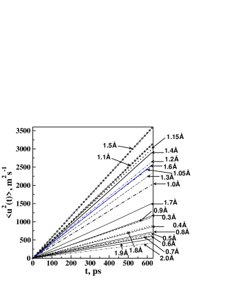
Figure 3: Mean square displacement as a function of time of the solutes of various sizes diffusing in a bcc solid.

Figure 3 shows the mean square displacement (MSD) for various solute sizes. We see that the curves are straight suggesting good statistics. The diffusivities are obtained from the slope of MSD data using Einstein’s relationship and these are plotted as a function of solute size in Figure 4. The diffusivity of solute initially decreases with increase in size of solute. Then there is a gradual increase in diffusivity with increase in solute size as can be seen from size 0.7Å onwards with a diffusivity maximum at 1.1Å. On further increase in solute diameter, there is a decrease in diffusivity which is followed by an increase in diffusivity once again for size 1.4Å and a second diffusivity maximum is observed for solute size 1.5Å. The diffusivity of 1.5Å solute is slightly higher than that of 1.1Å. The diffusivity of solutes larger than 1.5Å sharply decrease with size.

Figure 4: Self diffusivity, $D$ as a function of size of solute, $\sigma_{uu}$. There are diffusivity maxima at 1.1Å and 1.5Å.

Diffusion of a relatively small solute within the solvent made up of large-sized atoms occurs through jumps from one void to another neighbouring void. Two neighbouring voids are connected through a narrower region which is referred to as neck. Passage through the neck indeed forms the bottleneck for diffusion. The motion of the solvent atoms is around their equilibrium positions this leads to a distribution of neck diameters, f($r_{n}$) instead of a unique value for the neck diameter. It may be necessary for the solvent atoms to move away from their equilibrium position to permit the solute to pass through the bottleneck. This leads to activation energy barriers for large solutes. Large here means solutes whose diameter is larger than the neck diameter of the void interconnecting two neighbouring voids.

We have computed the strain energy in b.c.c. solid for different sized solutes. A small system consisting of 432 solvent atoms in a b.c.c. solid with 5 solute atoms has been simulated at 5K to compute the strain energy. Position coordinates were stored at an interval of 250fs for 500ps. Two sets of simulations were carried out, one in which the solvent atoms were not included in the molecular dynamics simulations (and therefore they were rigid) and another in which the solvent atoms were included in the integration along with the solute atoms. The average solute-solvent interaction energy is calculated in the case of rigid as well as flexible solvent runs. The difference in solute-solvent interaction energy in flexible and rigid host is the strain energy. Table 2 reports the solute-solvent interaction of various solute atoms and the strain energy. We note that the strain energy is generally small unless the solute diameter is large which is to be expected. Even for the largest sized solute of 1.8Å which is well beyond the size for which the diffusivity maximum was found in our simulations, the stain energy is about 10% of the total solute-solvent energy. Thus, in the regimes which are relevant to the present study and the regime where the diffusivity maximum is seen the contribution from the strain energy is not more than 16%. Most studies in the literature including those that were discussed in the introduction mainly concern large solutes where strain energy is important but for the present work, it plays only a secondary role, if at all. From this it is clear that although strain energy might be responsible for decrease in the diffusivity after the diffusivity maximum, diffusivity maximum does not have its origin in the strain energy.

Table 2: Strain energy of solute atoms in linear and anomalous regimes.

$\sigma_{uu}$,	Regime	$U_{uv}$(flexible host)	$U_{uv}$(rigid host)	Strain energy
Å		kJ/mol	kJ/mol	kJ/mol
0.5	Linear	-2.7430	-2.7660	0.023
0.6	Linear	-2.8334	-2.8132	-0.0202
0.9	Linear	-2.4911	-2.4704	-0.0207
1.1	Anomalous	-4.4226	-3.5568	-0.8658
1.3	Linear	-5.7127	-5.3544	-0.3583
1.5	Anomalous	-7.3439	-6.6290	-0.7149
1.8	Linear	-11.2414	-9.9361	-1.3053

Before we analyse the results that might lead to an understanding of the diffusivity maximum, we discuss the influence of the solute-solvent interaction energy on the diffusivity maximum.

4.1 Two distinct diffusivity maxima

There are previous reports of the existence of diffusivity maximum as a function of diffusants confined to other condensed matter phases such as porous solids, liquids, amorphous solids, etc [18, 8, 3, 12]. However, this is the first time that such a maximum has been reported for body-centred cubic close-packed solid. These studies have invariably reported a single diffusivity maximum as a function of the size of the diffusant. But here we find two maxima which has not been reported previously. It is therefore of considerable interest to investigate when and how such twin maxima are seen.

It is well known that solute-solvent interaction plays an important role in giving rise to anomalous diffusivity maximum. For example, it has been demonstrated unambiguously that the the size dependent diffusivity maximum of solute disappears in the absence of attractive interaction between the solute and solvent medium.[18, 11] Further, it has been shown that the diffusivity maximum disappears when the magnitude of the diffusant-medium (in the present case solute-solvent) interaction is small relative the kinetic energy, $k_{B}T$. We have therefore carried out simulations with different values of $\epsilon_{uv}$, the solute-solvent interaction strength. Simulations were carried out on a smaller system consisting of 686 solvent and 68 solute atoms at 70K. The position coordinates were stored once every 2ps.

Figure 5: Size dependent diffusivity of solute atoms as a function of solute-solvent interaction, $\epsilon_{uv}$ in rigid and flexible bcc solid, flexible fcc solid and dense fluid.

The diffusivity of solutes as a function of solute size is plotted in Figure 5. In case of flexible bcc host, $\epsilon_{uv}$ has been varied over the range 1.5-4.0 kJ/mol. Although there are two maxima (at 1.1 and 1.4Å) for $\epsilon_{uv}$ = 1.5 kJ/mol, the prominent maximum is for 1.1Å. With increase in interaction strength, the second maxima at 1.5Å gradually becomes the predominant maxima. We have carried out, simulations with flexible b.c.c. solid as well as rigid (when the solvent atoms were not included in MD integration). The effect of increase in $\epsilon_{uv}$ on D-$\sigma$ is same. However, the effect of rigid b.c.c. lattice is to shift the $\sigma$ at which maxima is seen to the right by 0.1Å: that is, the maxima are now seen at 1.2 and 1.6Å. In order to see if this effect of $\epsilon_{uv}$ always leads to appearance of a second maxima which further gains in strength, we carried out simulations on face-centred cubic (f.c.c.) solid solvent as well. The simulations have been carried out on at a reduced density of 0.933 with 500 solvent and 50 solute atoms and ($\epsilon_{vv}$=1.2kJ/mol, $\epsilon_{uv}$=3.0kJ/mol, $\epsilon_{uu}$=0.4kJ/mol, $\sigma_{vv}$=4.5Å). The melting point of this f.c.c. solid is 160K. Coordinates were accumulated every 250fs to obtain various properties. These results are also shown in Figure 5. We see that a single maximum is seen for low $\epsilon_{uv}$ while for $\epsilon_{uv}$ = 4.5 kJ/mol, there are two diffusivity maxima. The positions of these are precisely the same as the b.c.c. solid : 1.1 and 1.5Å. We also carried out simulations of liquid at 160K when the f.c.c. solid melts with same parameters as the f.c.c. solid. These results are also shown in Figure 5. Note that the for $\epsilon_{uv}$ = 4.5 kJ/mol there is single maximum. This is expected since at high temperatures, there is significant dynamical disorder. By 7.5 kJ/mol, we see that another maxima is developing around 1.4Å. The principal results of these set of simulations are : (i) at sufficiently high $\epsilon_{uv}$ two diffusivity maxima instead of the previously observed single maximum has been seen. (ii) this result is valid irrespective of the solvent structure (b.c.c. or f.c.c.) (iii) in the fluid phase, it is seen that two maxima are seen only at values of $\epsilon_{uv}$ that are higher than required for the solid phase. Further investigations are necessary to understand the role of $\epsilon_{uv}$ as well as distribution of neck diameters, f($r_{n}$) on diffusivity maxima.

4.2 Related aspects of diffusivity maximum

In order to understand the motion that leads to anomalous diffusivity maximum for certain solute sizes, we have obtained several other properties. The properties of anomalous regime solute sizes are compared with the properties of solutes which are not part of the maximum. These solutes are those belonging to the region where self diffusivity decreases with increase in solute diameter. This regime is referred to as the linear regime.

Figure 6: Velocity autocorrelation plot of solute atoms in linear (0.4, 1.0, 1.4)Å and anomalous (1.1, 1.5)Å regime.

Figure 6 displays the velocity autocorrelation function (VACF) for solute atoms in linear and anomalous regime. Solute from the linear regime shows an oscillatory VACF whereas solute from anomalous regime exhibits a smoothly decaying VACF without any backscattering. We attribute the presence of backscattering to the fact that the solute from linear regime encounters an energy barrier. Until it has enough energy to overcome the barrier, it performs oscillatory motion. Later, we will see how such a barrier arises. The VACF of 1.5Å decays faster in the initial time period and also exhibits a smoother decay as compared to 1.1Å solute.

The average mean square force acting on the solute atoms due to the solvent atoms is shown in Figure 7. The anomalous regime solute atoms experience lower average mean square force as compared to linear regime solute atoms. When the size of solute is very small as compared to the bottleneck diameter, it feels a large net force due to the neighboring solvent atoms in the neck region. The linear regime solute is thus bound and has a lower diffusivity. The anomalous regime solute has a diameter comparable to the neck diameter. For this reason, during its passage through the neck of the solute from anomalous regime, the centre of mass of the solute coincides with the centre of the bottleneck. By symmetry, the force exerted by the solvent atoms in a given direction is equal and opposite to the force exerted along diagonally opposite direction. This results in a mutual cancellation of forces leading to lower net force. The average mean square force on 1.1Å solute is smaller than solute of size 1.5Å though diffusivity of 1.5Å is higher than 1.1Å. This result is important since it suggests for the first time that there are factors other than mean square force that influence the diffusivity. We will see what these may be.

Figure 7: Average mean square force acting on the solute atoms due to the solvent atoms.

The diffusivity of a solute depends crucially on its activation energy. Therefore, we have computed $D$ at several temperatures. Arrhenius plot of linear and anomalous regime solute atoms from the diffusivities at four different temperatures (60, 80, 100 and 140K) for different solute sizes is shown in Figure 8.

Figure 8: Arrhenius plot for solute atoms in linear and anomalous regime obtained from diffusivities at 60, 80, 100 and 140K.

The activation energy of the solute atoms obtained from the slope of Arrhenius plot are listed in Table 3. The activation energy of linear regime solute atoms is larger than anomalous regime solute atoms. Further, activation energy of 1.5Å solute is lower than 1.1Å which is consistent with the observed higher diffusivity of 1.5Å solute as compared to 1.1Å. Thus, it appears that the activation energy is responsible for the observed differences in self diffusivity as a function of the size. In particular, the difference in the self diffusivity of the solutes located at the two maxima can be explained in terms of the difference in the activation energy for these two solute sizes.

Table 3: Activation Energy of solute atoms in linear and anomalous regimes.

$\sigma_{uu}$, Å	Regime	$E_{act}$, kJ/mol
0.6	linear	2.5333
1.1	anomalous	1.0659
1.5	anomalous	0.9096

4.3 Physical picture of motion of the solute

More detailed behaviour of the motion of the solute can be gleaned from the wavenumber dependence of various properties. The self part of the intermediate scattering function, $F_{s}$(k,t) has been computed from the molecular dynamics data.

Figure 9: -ln($F_{s}$(k,t)) as a function of time for linear (0.6, 0.9)Å and anomalous (1.1, 1.5)Å regime solute atoms for motion within b.c.c. solid.

The natural logarithm of $F_{s}$(k,t) as a function of time for solute atoms in both the linear and anomalous regimes is reported in Figure 9. The inverse of the slope of -ln($F_{s}$(k,t)) as a function of time gives the relaxation time. In case of linear regime solute atoms, there are two slopes corresponding to two relaxation times whereas anomalous regime solute atoms show only one slope and one relaxation time. This suggests that the solute atom from the linear regime performs two distinct type of motion while anomalous regime impurity atom performs only one type of motion.

The physical picture regarding the motion performed by solutes in these regimes is similar to that proposed by Singwi and Sjölander [14] for solute motion in water. Water molecules diffuse much more slowly in water than the solute and this is similar to the present situation where the solvent molecules are slow while the solute motion is fast. The model due to Singwi and Sjölander envisages that the solute performs an oscillatory motion for a short period of time, $\tau_{1}$ before it performs a diffusive motion on the time scale $\tau_{2}$. This leads to biexponential decay and applies to linear regime solute. We suggest that the linear regime solute performs oscillatory motion initially when it is confined in the solvent shell for a given time. Once it overcomes the energy barrier to move past the solvent shell it performs motion with relaxation time $\tau_{2}$. The anomalous regime solute does not feel the energy barrier at the solvent shell and thus finds the region within the solvent shell and region outside the solvent shell similar. It, thus, sees a homogeneous solvent rather than two distinct, heterogeneous regions - one inside the solvent shell and another outside - seen by the solute from linear regime. The relaxation times of different solute atoms are reported in Table 4.

Table 4: Relaxation times of solute atoms in linear and anomalous regimes for wavevector 0.2428Å.

$\sigma_{uu}$, Å	Regime	$\tau_{1}$, ps	$\tau_{2}$, ps
0.6	Linear	31.25	218.44
0.9	Linear	23.53	83.33
1.1	Anomalous	26.00
1.5	Anomalous	19.23

The relaxation time for anomalous regime solute atom is less than the linear regime solute atom. Further, the relaxation of 1.5Å solute is faster than 1.1Å. This is consistent with both the lower activation energy and the relative magnitudes of self diffusivities.

The Fourier transformation of self part of the intermediate scattering function gives the dynamic structure factor, $S_{s}$(k,$\omega$). In the hydrodynamic limit, full width at half maximum (fwhm) $\Delta\omega$(k) of dynamic structure factor is 2D$k^{2}$. The ratio $\Delta\omega(k)/2Dk^{2}$ provides an idea of the $k$ dependence of self diffusivity. This ratio, $\Delta(k)$ is shown in Eq. 4

$$\Delta(k)=\frac{\Delta\omega(k)}{2Dk^{2}}$$ (4)

Figure 10: $\Delta$(k) as a function of wavevector, k for linear and anomalous regime solute atoms.

We have obtained the $\Delta$(k) for different wavenumbers for the solute atoms in linear and anomalous regimes using the width of dynamic structure factor and is shown in Figure 10. The width, $\Delta$(k) shows oscillatory behavior for linear regime solute atoms and nearly monotonic decay of $\Delta$(k) for anomalous regime solute atoms. The minimum seen for $k$ around 1.2Å^-1 for 0.9Å solute arises from the slowing down of the self diffusivity on these length scales. $k$ = 1.2Å^-1 approximately corresponds to the position where the first neighbour shell is located. These are in good agreement with the results for liquid argon at low and high densities by Nijboer and Rahman [7] as well as Levesque and Verlet [6] as well as the discussions in Boon and Yip [1]. The anomalous regime solute does not experience any barrier to exit from the first solvent shell and therefore shows a nearly smooth decay of $\Delta$(k) with wavenumber.

5 Conclusions

The present study suggests that there is a maximum in self diffusivity for solutes diffusing within the interstitial space provided by a body-centred cubic solid. The maxima are seen when the solute/solvent size ratio is in the range 0.25-0.33. We report, for the first time, the existence of more than one maximum in self diffusivity as a function of the size of the solute. We show that two maxima are seen when the solute-solvent interaction strength is large. It is seen that two maxima are also seen in face-centred cubic arrangement as well as in liquids. For the latter, two maxima are seen when the solute-solvent interaction strength is higher relative to diffusion in solids. Further, we show that the relative heights of the two maxima are determined by the activation energies. We emphasize that the present study does not study the regime of large solutes where strain energy becomes important. In previous studies, it was thought that distribution of bottleneck diameter alone had a role in determining the diffusivity maximum. The present study suggests that in addition to f($r_{n}$), solute-solvent interaction strength also influences the observed size dependence of self diffusivity on diameter of the solute.

Acknowledgment : Authors wish to thank Department of Science and Technology, New Delhi for financial support in carrying out this work. Authors also acknowledge C.S.I.R., New Delhi for a research fellowship to M.S.

References

- [1] J. P. Boon and Sidney Yip. Molecular Hydrodynamics. Dover Publications, New York, 1980.
- [2] A. Ferro. J. Appl. Phys., 28:895, 1957.
- [3] Pradip Kr. Ghorai and S. Yashonath. The stokes-einstein relationship and the levitation effect: Size dependent diffusion maximum in dense fluids and close-packed disordered solids. J. Phys. Chem. B, 109:5824, 2005.
- [4] G. M. Hood. J. Phys. F: Metal Phys., 6:19, 1976.
- [5] Sung-Yul Lee, Y. Iuima, and K. Hirano. Phys. Sat. Sol.(a), 136:311, 1993.
- [6] D. Levesque and L. Verlet. Phys. Rev. A, 2:2514, 1970.
- [7] B. R. A. Nijboer and A. Rahman. Physica, 32:415, 1966.
- [8] P. K. Padmanabhan and S. Yashonath. J. Phys. Chem., 106:3443, 2002.
- [9] M. Parrinello and A. Rahman. Phys. Rev. Lett., 45:1196, 1980.
- [10] M. Parrinello, A. Rahman, and P. Vashishta. Phys. Rev. Lett., 50:1073, 1983.
- [11] M. Sharma and S. Yashonath. J. Phys. Chem. B, 110:17217, 2006.
- [12] M. Sharma and S. Yashonath. J. Chem. Phys., 129:144103, 2008.
- [13] Wei-Mei Shyu, K. S. Singwi, and M. P. Tosi. Phys. Rev. B, 3:271, 1971.
- [14] K. S. Singwi and A. Sjölander. Phys. Rev., 119:863, 1960.
- [15] W. Smith and T.R. Forester. The DL-POLY-2.13. CCLRC, Daresbury Laboratory, Daresbury, UK, 2001.
- [16] P. Vashishta and A. Rahman. Phys. Rev. Lett., 40:1337, 1978.
- [17] S. Yashonath and C. N. R. Rao. Mol. Phys., 54:245, 1985.
- [18] S. Yashonath and P. Santikary. J. Phys. Chem., 98:6368, 1994.