Finite Temperature Phase Diagram in Rotating Bosonic Optical Lattice

Abstract

Finite temperature phase boundary between superfluid phase and normal state is analytically derived by studying the stability of normal state in rotating bosonic optical lattice. We also analytically prove that the oscillation behavior of critical hopping matrix directly follows the upper boundary of Hofstadter butterfly as the function of effective magnetic field.

PACS number(s): 03.75.Lm, 05.30.Jp, 73.43.Nq

1 Introduction

Bose-Hubbard model of interacting bosons on a lattice has been used to describe superfluid-Mott insulator (MI) phase transition in a variety of systems at zero temperature, e.g., Josephson arrays and granular superconductors [1]. The recent suggestion to experimentally observe this transition in a system of cold bosonic atoms in an optical lattice [2] and its successful experimental demonstration [3] have aroused much theoretical [4, 5, 6] and experimental [7, 8] interest in this model, especially rotating optical lattice has also become brand-new topics in bosonic system. Most of work about rotating optical lattice focused on the superfluid phase and studied the pinning effect of the vortex lattice due to optical periodic potential [9, 10, 11, 12]. The similar question has been investigated in the type-$\Pi$ superconductor [13, 14, 15, 16].

However the question of superfluid-MI phase transition at zero temperature still exists in rotating optical lattice and the phase diagram at zero temperature has been achieved by strong coupling expansion [17] and Gutzwiller approach [18, 19]. Strong coupling expansion obtained the phase boundary between the superfluid phase and MI by perturbatively computing the energy difference between MI and single-charge excitation states on top of the MI. This method is very accurate and applicable to the random dimension but is not suitable for system in deep superfluid phase where the perturbation is not valid any longer. Gutzwiller approach is at the self-consistent mean-field level and based on an ansatz that many-body ground state factorizes into product of single lattice site wave function. So under this approximation the system become diagonal with respect to the lattice site and we can use an effective single-site Hamiltonian. The disadvantage of Gutzwiller approach is that it fails to describe the correct short-range correlation between different lattice sites and so is an uncontrolled approximation. However, Gutzwiller approach can predict a qualitatively similar phase diagram with strong coupling expansion [18].

In this paper, we mainly extend the phase diagram of a rotating two-dimensional bosonic optical lattice to finite temperature utilizing the Gutzwiller mean-field theory. At finite temperature, MI is replaced by normal state which possesses finite compressibility. Here we do not include the crossover from MI to normal state at finite temperature since there is not an conventional definition for this crossover as far as what we know is concerned. So at finite temperature the phase transition happens between superfluid phase and normal state instead of MI. In section 2, by making an analogy between rotating optical lattice and electrons constrained by periodic potential and external magnetic field, we qualitatively derive the Bose-Hubbard Hamiltonian in rotating optical lattice. In section 3, we follow the method used in [20] to analytically locate the phase boundary of superfluid phase and normal state by discussing the stability of fixed point corresponding to the normal state and in section 4 a brief conclusion is given.

2 Bose-Hubbard Hamiltonian in Rotating Optical Lattice

We consider a two-dimensional bosonic system in $XY$ plane restricted by a square optical lattice and an harmonic trapping potential which have a common rotating velocity $\Omega$ along $Z$ axis. In the laboratory frame, the potential is generally time-dependent. It is therefore convenient to transform to the frame rotating with the potential, since in that frame the potential is constant in time, and thus the standard methods for finding the equilibrium may be employed. In the frame of rotating potential, the second quantized Hamiltonian for a particle of mass $m$ in an harmonic trap of natural frequency $\omega$ can be written into $H=H_{0}+H_{I}$ with

$$H_{0} = \int d\,\vec{R}\,\Psi^{{\dagger}}(\vec{R})\left(-\frac{\hbar^{2}\nabla^{2}}{2m}+V_{L}(\vec{R})+\frac{1}{2}m\omega^{2}R^{2}-\Omega L_{Z}-\mu\right)\Psi(\vec{R})$$ (1)

$$H_{I} = \frac{g}{2}\int d\,\vec{R}\,\Psi^{{\dagger}}(\vec{R})\Psi^{{\dagger}}(\vec{R})\Psi(\vec{R})\Psi(\vec{R})$$ (2)

where $L_{Z}=-i\hbar(X\partial_{Y}-Y\partial_{X})$ is angular momentum along $Z$ axis and $g(>0)$ is the strength of contact interaction potential between two particles. $V_{L}(\vec{R})$ is periodic optical potential and $\Psi(\vec{R})$ is field operator for boson particles. The term involving the chemical potential $\mu$ is added because it is very convenient to be in the grand canonical ensemble. $H_{0}$ can be rearranged into

$$H_{0}=\int d\,\vec{R}\,\Psi^{{\dagger}}(\vec{R})\left[\frac{(-i\hbar\nabla-e/c\vec{A}(\vec{R}))^{2}}{2m}+V_{L}(\vec{R})+\frac{1}{2}m(\omega^{2}-\Omega^{2})R^{2}-\mu\right]\Psi(\vec{R})$$ (3)

where $\vec{A}(\vec{R})=mc/e\vec{\Omega}\times\vec{R}$ is an effective vector potential with $c$ and $e$ representing light speed and charge quanta. This form suggests that the effects of rotation are partitioned into two different parts. The term $1/2m(\omega^{2}-\Omega^{2})R^{2}$ implies that the centrifugal potential weakens the role of trapping potential (in order to stabilize the system, $\Omega\leq\omega$). The other part of rotation is included in the first term whose role is producing an effective magnetic field $\vec{B}=\nabla\times\vec{A}(\vec{R})=2mc/e\vec{\Omega}$ and provides a structure of Landau level for atoms. Hence at this point we can draw a conclusion that the motion of atoms in a rotating optical lattice under the assumption $\omega=\Omega$ is completely the same as that of electrons constrained by periodic potential and external magnetic field. Therefore the method utilized to deal with electrons can be applicable to the our problem. For simplicity, below we assume $\omega=\Omega$ so that the centrifugal force accurately compensates the harmonic trapping potential.

For systems without rotation and trap potential ($\Omega=\omega=0$) we usually assume that the atoms are cooled within the lowest Bloch band and the field operator can be expanded into $\Psi(\vec{R})=\sum_{i}b_{i}w(\vec{R}-\vec{R}_{i})$ in terms of the lowest Wannier function $w(\vec{R}-\vec{R}_{i})$ with $b_{i}$ being bosonic annihilation operator at the lattice site $\vec{R}_{i}$. Hence the system is sufficiently described by a single-band Bose-Hubbard Hamiltonian [2]

$$H = -t\sum_{<ij>}b_{i}^{{\dagger}}b_{j}+\frac{U}{2}\sum_{i}b_{i}^{{\dagger}}b_{i}^{{\dagger}}b_{i}b_{i}-\mu\sum_{i}b_{i}^{{\dagger}}b_{i}$$ (4)

where $t=-\int d\vec{R}\,w^{\ast}(\vec{R}-\vec{R}_{i})\left[-\frac{\hbar^{2}\nabla^{2}}{2m}+V_{L}(\vec{R})\right]w(\vec{R}-\vec{R}_{j})$ is hopping matrix restricted to nearest neighbors and $U=g\int d\vec{R}\,|w(\vec{R}-\vec{R}_{i})|^{4}$ is on-site interaction strength. When external effective magnetic field appears, many-band effects must be considered which leads to that single-band Bose-Hubbard Hamiltonian is not valid any more. Fortunately from the study of lattice electron in external magnetic field [21] we know that there exists an effective single-band Hamiltonian which can be obtained from (4) by only making a substitution for hopping matrix

$$H=-t\sum_{<ij>}\exp{\left[\frac{ie}{\hbar c}\int_{\vec{R}_{j}}^{\vec{R}_{i}}\vec{A}(\vec{R})\cdot d\vec{R}\right]}b_{i}^{{\dagger}}b_{j}+\frac{U}{2}\sum_{i}b_{i}^{{\dagger}}b_{i}^{{\dagger}}b_{i}b_{i}-\mu\sum_{i}b_{i}^{{\dagger}}b_{i}$$ (5)

The added phase factor is called Peierls phase factor. It is well known that superfluid-MI phase transition comes from the competition between hopping matrix and on-site interaction strength [3]. But when the magnetic field is introduced the on-site interaction strength is unchanged while the hopping matrix is modified, so we naturally expect a modified phase boundary between superfluid and MI.

The vector potential $\vec{A}(\vec{R})$ in the symmetric gauge concerns the $X$ and $Y$ components of coordinate at the same time and makes below calculation be more complex. We hope only $X$ or $Y$ component is concerned, which is realized by making a canonical transformation to field operator

$$b_{i}\longrightarrow b_{i}\exp{\left[\frac{ie}{\hbar c}\int_{\vec{R}_{i}}^{\vec{R}_{l}}mc/e\vec{\Omega}\times\vec{\underline{R}}\cdot d\vec{R}\right]}$$ (6)

with $\vec{\underline{R}}=(X,-Y)$ and $\vec{R}_{l}$ being a arbitrary reference point. Under this transformation

$$H=-t\sum_{<ij>}\exp{\left[i2\pi\phi\int_{\vec{r}_{j}}^{\vec{r}_{i}}xdy\right]}b_{i}^{{\dagger}}b_{j}+\frac{U}{2}\sum_{i}b_{i}^{{\dagger}}b_{i}^{{\dagger}}b_{i}b_{i}-\mu\sum_{i}b_{i}^{{\dagger}}b_{i}$$ (7)

where all the coordinates are scaled by the lattice constant $a$ hence are dimensionless. $\phi=Ba^{2}/(hc/e)$ represents the number of magnetic flux quanta penetrating the unit cell. In fact it is easy to find that the above Hamiltonian corresponds to that in Landau gauge $\vec{A}(\vec{R})=BX\hat{Y}$ with $\hat{Y}$ denoting the unit vector along the $Y$ axis. In the next section, we will regard the Hamiltonian (7) as our starting point and study its phase diagram at finite temperature at mean-field level.

3 Phase Diagram in Gutzwiller Mean-Field Approach

The Gutzwiller approach is a self-consistent mean-field method and equivalent to the decoupling approximation [22, 23] to the hopping term

$$b_{i}^{{\dagger}}b_{j} = <b_{i}^{{\dagger}}>b_{j}+b_{i}^{{\dagger}}<b_{j}>-<b_{i}^{{\dagger}}><b_{j}>$$ (8)

$$= \alpha_{i}b_{j}+b_{i}^{{\dagger}}\alpha_{j}-\alpha_{i}\alpha_{j}$$

where $\alpha_{i}=\alpha_{i}^{\ast}$ is superfluid order parameter which distinguishes the superfluid phase from normal state. If magnetic field vanishes, the whole system is uniform and order parameter is also site-independent. But we can not suppose this when the magnetic field appears. After this decoupling, the system is describable in terms of a single-site Hamiltonian

$$H_{nm} = -t\left[b_{nm}^{{\dagger}}\left(\alpha_{(n+1)m}+\alpha_{(n-1)m}+e^{-i2\pi n\phi}\alpha_{n(m+1)}+e^{i2\pi n\phi}\alpha_{n(m-1)}\right)+H.C.\right]+$$ (9)

$$\frac{U}{2}b_{nm}^{{\dagger}}b_{nm}^{{\dagger}}b_{nm}b_{nm}-\mu b_{nm}^{{\dagger}}b_{nm}$$

where we label site of the lattice $i$ by two ordered integers $i=(n,m)$, the first integer along the $X$ axis and the second one along the $Y$ axis. In the Landau gauge, hopping along the $Y$ axis achieves the Peierls phase factor and that along $X$ axis is invariant. The above Hamiltonian has two striking characteristics [18]. On the one hand, it is independent of $Y$ component, so the translational symmetry along $Y$ axis is conservative and we can suppose order parameter $\alpha_{nm}=\alpha_{n}$ in correspondence with the case without magnetic field. On the other hand although it depends on $X$ component, for rational $\phi=p/q$ ($p,q$ have no common factor), q-site translational symmetry along $X$ axis is recovered $\alpha_{n}=\alpha_{n+q}$. So the Hamiltonian is further reduced into

$$H_{n} = -t\left[b_{n}^{{\dagger}}\left(\alpha_{n+1}+\alpha_{n-1}+2\alpha_{n}\cos{2\pi n\phi}\right)+H.C.\right]+\frac{U}{2}b_{n}^{{\dagger}}b_{n}^{{\dagger}}b_{n}b_{n}-\mu b_{n}^{{\dagger}}b_{n}$$ (10)

with $n$ being integer from $1$ to $q$. In addition, the Hamiltonian is periodic as the function of magnetic field $H_{n}(\phi)=H_{n}(\phi+K)$ with $K$ being a random integer so that we only need consider $\phi\in[0,1)$. Note also that in (9) and (10) we have neglected a constant term which does not influence our result.

The self-consistency of Gutzwiller method must be carried out by the condition

$$\alpha_{n}=\frac{1}{Z_{n}}Tr\left(b_{n}e^{-\beta H_{n}}\right)=\frac{1}{Z_{n}}Tr\left(b_{n}^{{\dagger}}e^{-\beta H_{n}}\right)$$ (11)

with $\beta=1/(K_{B}T)$ and partition function $Z_{n}=Tr\exp{(-\beta H_{n})}$. Introducing the same notation in [20] $\gamma_{n}=t\alpha_{n}$, self-consistent condition can be rewritten into

$$\gamma_{n}=\frac{t}{6\beta}\left(\frac{\partial}{\partial\gamma_{n+1}}+\frac{\partial}{\partial\gamma_{n-1}}+\frac{1}{2\cos{2\pi n\phi}}\frac{\partial}{\partial\gamma_{n}}\right)\ln{Z_{n}}$$ (12)

Under Gutzwiller approximation the eigenstates of $H_{n}$ can be expanded in terms of Fock state, then we diagonalize this Hamiltonian matrix under Fock basis truncated until a given number of particle $N$ to obtain the eigenvalues $E_{l}$ ($l=0,1,\cdot\cdot\cdot,N$) which are function of $\gamma_{n-1},\gamma_{n}$ and $\gamma_{n+1}$. So we proceed using the eigenvalues

$$\gamma_{n}=-\frac{t}{6}\sum_{l=0}^{N}e^{-\beta E_{l}}\left(\frac{\partial E_{l}}{\partial\gamma_{n-1}}+\frac{\partial E_{l}}{\partial\gamma_{n+1}}+\frac{1}{2\cos{2\pi n\phi}}\frac{\partial E_{l}}{\partial\gamma_{n}}\right)/\sum_{l=0}^{N}e^{-\beta E_{l}}$$ (13)

The derivative of eigenvalue is computable from the characteristic polynomial $P(\lambda,\gamma_{n-1},\gamma_{n},\gamma_{n+1})$ of Hamiltonian matrix [24]

$$\frac{\partial E_{l}}{\partial\gamma_{i}} = -\frac{\partial P(E_{l},\gamma_{n-1},\gamma_{n},\gamma_{n+1})}{\partial\gamma_{i}}/\frac{\partial P(E_{l},\gamma_{n-1},\gamma_{n},\gamma_{n+1})}{\partial E_{l}}$$

$$\frac{\partial P(E_{l},\gamma_{n-1},\gamma_{n},\gamma_{n+1})}{\partial E_{l}} = \sum_{k=0}^{N}P^{(k)}(E_{l},\gamma_{n-1},\gamma_{n},\gamma_{n+1})$$

$$\frac{\partial P(E_{l},\gamma_{n-1},\gamma_{n},\gamma_{n+1})}{\partial\gamma_{n-1}} = 2(\gamma_{n-1}+\gamma_{n+1}+2\gamma_{n}\cos{2\pi n\phi})\cdot$$

$$\left[\sum_{k=1}^{N}kP^{(k,\,k-1)}(E_{l},\gamma_{n-1},\gamma_{n},\gamma_{n+1})+Q(\gamma_{n-1},\gamma_{n},\gamma_{n+1})\right]$$

$$\frac{\partial P(E_{l},\gamma_{n-1},\gamma_{n},\gamma_{n+1})}{\partial\gamma_{n+1}} = \frac{\partial P(E_{l},\gamma_{n-1},\gamma_{n},\gamma_{n+1})}{\partial\gamma_{n-1}}$$

$$\frac{\partial P(E_{l},\gamma_{n-1},\gamma_{n},\gamma_{n+1})}{\partial\gamma_{n}} = 2\cos{2\pi n\phi}\frac{\partial P(E_{l},\gamma_{n-1},\gamma_{n},\gamma_{n+1})}{\partial\gamma_{n-1}}$$ (14)

where the notation $P^{\{k\}}(E_{l},\gamma_{n-1},\gamma_{n},\gamma_{n+1})$ denotes the characteristic polynomial of the matrix obtained by discarding from Hamiltonian matrix the rows and columns labeled by the set of indices $\{k\}$ and the polynomial $Q(\gamma_{n-1},\gamma_{n},\gamma_{n+1})$ satisfies $Q(0,0,0)=0$. Substituting all above relations into (13)

$$\gamma_{n} = t(\gamma_{n-1}+\gamma_{n+1}+2\gamma_{n}\cos{2\pi n\phi})\frac{\sum_{l=0}^{N}e^{-\beta E_{l}}W(E_{l},\gamma_{n-1},\gamma_{n},\gamma_{n+1})}{\sum_{l=0}^{N}e^{-\beta E_{l}}}$$

$$W(E_{l},\gamma_{n-1},\gamma_{n},\gamma_{n+1}) = \frac{\sum_{k=1}^{N}kP^{(k,\,k-1)}(E_{l},\gamma_{n-1},\gamma_{n},\gamma_{n+1})+Q(\gamma_{n-1},\gamma_{n},\gamma_{n+1})}{\sum_{k=0}^{N}P^{(k)}(E_{l},\gamma_{n-1},\gamma_{n},\gamma_{n+1})}$$ (15)

Until now, we have obtained the equation set of self-consistently deciding all order parameters. If order parameters have nonzero solution the system is in superfluid phase. If order parameters have zero solution, the system is in normal state. So we can determine the phase boundary between superfluid phase and normal state by studying the stability of the fixed point corresponding to the normal state ($\gamma_{n}=0$ for all $n$) [20]. According to a standard theory, the stability of such a fixed point can be discussed based on the spectrum of the matrix linearizing the map defined by equation set (15) in the vicinity of normal state. Linearizing (15) around the fixed point of normal state, we obtain

$$\gamma_{n} = t\Theta(U,\mu,\beta)(\gamma_{n-1}+2\gamma_{n}\cos{2\pi n\phi}+\gamma_{n+1})$$ (16)

$$\Theta(U,\mu,\beta) = \frac{\sum_{l=0}^{N}e^{-\beta\left(U/2l(l-1)-\mu l\right)}W(U/2l(l-1)-\mu l,0,0,0)}{\sum_{l=0}^{N}e^{-\beta\left(U/2l(l-1)-\mu l\right)}}$$ (17)

Writing above equations in the form of matrix if we denote $\Upsilon=(\gamma_{1},\gamma_{2},\cdot\cdot\cdot\gamma_{q})^{t}$

$$\Upsilon = t\Theta(U,\mu,\beta)M(\phi)\Upsilon$$

$$M(\phi) = \left(\begin{array}[]{cccccc}2\cos{2\pi\phi}&1&0&\cdot\cdot\cdot&0&1\\ \vskip 3.0pt plus 1.0pt minus 1.0pt1&2\cos{4\pi\phi}&1&\cdot\cdot\cdot&0&0\\ \vskip 3.0pt plus 1.0pt minus 1.0pt\cdot\cdot\cdot&\cdot\cdot\cdot&\cdot\cdot\cdot&\cdot\cdot\cdot&\cdot\cdot\cdot&\cdot\cdot\cdot\\ \vskip 3.0pt plus 1.0pt minus 1.0pt1&0&0&\cdot\cdot\cdot&1&2\cos{2\pi q\phi}\end{array}\right)$$ (22)

Therefore, the fixed point of the normal state is stable only if the maximal eigenvalue $\epsilon_{max}(\phi)$ of $M(\phi)$ satisfies $t\Theta(U,\mu,\beta)\epsilon_{max}(\phi)<1$, which signifies that the phase transition between superfluid phase and normal state is

$$t\Theta(U,\mu,\beta)\epsilon_{max}(\phi)=1$$ (23)

This is our main result. At $T=0K$ only the eigenstate having the lowest energy contributes to the partition function. Easily proven when $\mu\in[l-1,l]$, the phase boundary at $T=0K$ is specified by

$$t=\frac{1}{\epsilon_{max}(\phi)}\frac{[\mu-U(l-1)][Ul-\mu]}{U+\mu}$$ (24)

which is the same as the result in [19, 25].

Below we connect $\epsilon_{max}(\phi)$ with the famous Hofstadter butterfly. We find that eigenvalues of the matrix $M(\phi)$ actually correspond to a part of energy spectrum of Hofstadter butterfly [26]. According to the proof in [19] that the maximal eigenvalue of $M(\phi)$ is equal to the maximal eigenvalue of Hofstadter butterfly, hence from (23) we find for fixed $U,\mu,\beta$ the critical hopping strength is inversely proportional to the maximal eigenvalue of Hofstadter butterfly. According to the fact that the maximal eigenvalue of Hofstadter butterfly shows an oscillatory behavior as the function of magnetic field [26], the critical hopping strength also exhibits the oscillation following the maximal eigenvalue, i.e. upper boundary of Hofstadter butterfly.

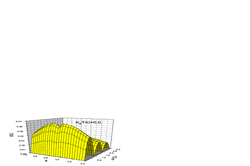
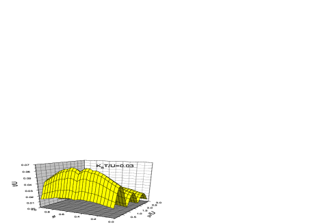
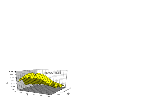
Figure 1: The three-dimensional phase diagram for different temperature $K_{B}T/U=0.0,0.03,0.08$. Below the critical surface is normal state.

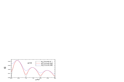
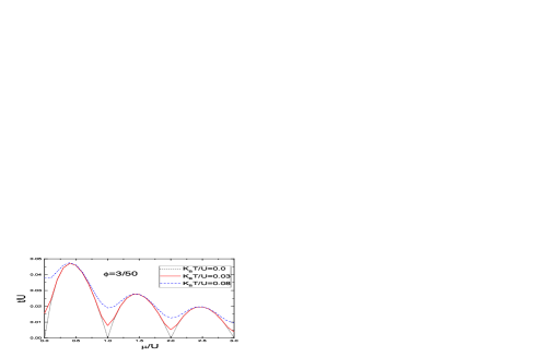
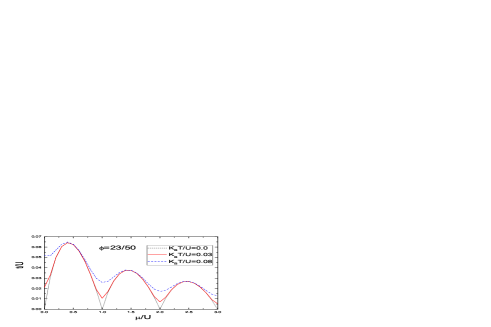
Figure 2: The two-dimensional phase diagram for different temperature and magnetic field. Below the critical line is normal state.

In Fig.1, we plot three-dimensional phase diagram for different temperature. When $T=0K$ the phase boundary separates the superfluid phase and MI, which is not true for finite temperature. In order to concentrate on the effects of temperature and magnetic field, we also plot the two dimension phase diagram for different temperature and magnetic field in Fig.2. Note that the phase boundary of $\phi=0$ is obtained by letting $\epsilon_{max}(0)=4$ [25, 26]. Seeing from the Fig.2, we could draw below conclusions. For fixed magnetic field the higher the temperature, the smaller the area of the superfluid phase, which is consistent with the fact that the high temperature destroys the superfluidity. At the same time for fixed temperature, magnetic field has a much more complex effect on the superfluidity in view of oscillatory behavior of critical hopping matrix. Generally speaking in contrast to the situation without the magnetic field, magnetic field always nonmonotonically increases the area of normal state, which can be illustrated from the bandwidth of Hofstadter butterfly. On the one hand the narrower the bandwidth, the smaller the effective hopping matrix. But the bandwidth of Hofstadter butterfly is often less than that without magnetic field [26]. Hence the effective hopping matrix is always less than $t$. On the other hand the on-site interaction strength is invariant. Considering the above two factors, we naturally understand the effect of magnetic field.

4 Conclusion

In conclusion we have qualitatively derived the Hamiltonian of rotating optical lattice, analytically extended the phase diagram of rotating Bose-Hubbard model to finite temperature and analyzed the relation between the oscillation behavior of critical hopping matrix and Hofstadter butterfly. In addition, we have also illustrated how the rotation influences the phase diagram.

Figure 3: The three-dimensional phase diagram for different temperature $K_{B}T/U=0.0,0.03,0.08$. Below the critical surface is normal state.

Figure 4: The two-dimensional phase diagram for different temperature and magnetic field. Below the critical line is normal state.

References

• [1] M. P. A. Fisher, P. B. Weichman, G. Grinstein and D. S. Fisher, Phys. Rev. B40, 546(1989).
• [2] D. Jaksch, C. Bruder, J. I. Cirac, C. W. Gardiner and P. Zoller, Phys. Rev. Lett. 81, 3108(1998).
• [3] M. Greiner, O. Mandel, T. Esslinger, T. W. HΓ€nsch and I. Bloch, Nature (London), 415, 39(2002).
• [4] M. S. Luthra, T. Mishra, R. V. Pai, and B. P. Das, Phys. Rev. B78, 165104 (2008).
• [5] A. ArgΓΌelles and L. Santos, Phys. Rev. A75, 053613(2007).
• [6] T. P. Polak and T. K. KopeΔ‡, Phys. Rev. B76, 094503(2007).
• [7] D. McKay, M. White, M. Pasienski and B. DeMarco, Nature (London), 453, 76(2008).
• [8] S. Trotzky, P. Cheinet, S. FΓΆlling, M. Feld, U. Schnorrberger, A. M. Rey, A. Polkovnikov, E. A. Demler, M. D. Lukin and I. Bloch, Science 319, 295(2008).
• [9] K. Kasamatsu and M. Tsublta, Phys. Rev. Lett. 97, 240404(2006).
• [10] R. Bhat, M. J. Holland and L. D. Carr, Phys. Rev. Lett. 96, 060405(2006).
• [11] H. Pu, L. O. Baksmaty, S. Yi and N. P. Bigelow, Phys. Rev. Lett. 94, 190401(2005).
• [12] J. W. Reijnders and R. A. Duine, Phys. Rev. Lett. 93, 060401(2004).
• [13] J. I. Martin, M. Velez, J. Nogues and I. K. Schuller, Phys. Rev. Lett. 79, 1929(1997).
• [14] D. J. Morgan and J. B. Ketterson, Phys. Rev. Lett. 80, 3614(1998).
• [15] V. Zhuravlev and T. Maniv, Phys. Rev. B68, 174507(2003).
• [16] W. V. Pogosov, A. L. Rakhmanov and V. V. Moshchalkov, Phys. Rev. B67, 014532(2003).
• [17] M. Niemeyer, J. K. Freericks and H. Monien, Phys. Rev. B60, 2357(1999).
• [18] M. Γ–. Oktel, M. Nitǎ and B. Tanatar, Phys. Rev. B75, 045133(2007).
• [19] R. O. Umucalilar and M. Γ–. Oktel, Phys. Rev. A76, 055601(2007).
• [20] P. Buonsante and A. Vezzani, Phys. Rev. A70, 033608(2004).
• [21] F. H. L. Essler, H. Frahm, F. GΓΆhmann, A. KlΓΌmper and V. E. Korepin, The One-Dimensioal Hubbard Model (Cambridge, 2005)
• [22] K. Sheshadri, H. R. Krishnamurthy, R. Pandit and T. V. Ramakrishnan, Europhys. Lett. 22, 257(1993).
• [23] D. V. Oosten, P. V. D. Straten and H. T. C. Stoof, Phys. Rev. A63, 053601(2001).
• [24] C. Meyer, Matrix Analysis and Applied Linear Algebra (SIAM, Philadelphia, 2001).
• [25] D. S. Goldbaum and E. J. Mueller, Phys. Rev. A77, 033629(2008).
• [26] D. R. Hofstadter, Phys. Rev. B14, 2239(1976).