Real Computation with Least Discrete Advice:
A Complexity Theory of Nonuniform Computability

Abstract

It is folklore particularly in numerical and computer sciences that, instead of solving some general problem $f:A\to B$, additional structural information about the input $x\in A$ (that is any kind of promise that $x$ belongs to a certain subset $A^{\prime}\subseteq A$) should be taken advantage of. Some examples from real number computation show that such discrete advice can even make the difference between computability and uncomputability. We turn this into a both topological and combinatorial complexity theory of information, investigating for several practical problems how much advice is necessary and sufficient to render them computable.
Specifically, finding a nontrivial solution to a homogeneous linear equation $A\cdot\vec{x}=0$ for a given singular real $n\times n$-matrix $A$ is possible when knowing $\operatorname{rank}(A)\in\{0,1,\ldots,n-1\}$; and we show this to be best possible. Similarly, diagonalizing (i.e. finding a basis of eigenvectors of) a given real symmetric $n\times n$-matrix $A$ is possible when knowing the number of distinct eigenvalues: an integer between $1$ and $n$ (the latter corresponding to the nondegenerate case). And again we show that $n$–fold (i.e. roughly $\log n$ bits of) additional information is indeed necessary in order to render this problem (continuous and) computable; whereas for finding some single eigenvector of $A$, providing the truncated binary logarithm of the least-dimensional eigenspace of $A$—i.e. $(\lfloor\log_{2}n\rfloor+1)$-fold advice—is sufficient and optimal.

1 Introduction

Recursive Analysis, that is Turing’s [Turi36] theory of rational approximations with prescribable error bounds, is generally considered a very realistic model of real number computation [BrCo06]. Much research has been spent in ‘effectivizing’ classical mathematical theorems, that is replacing mere existence claims

1. “for all $x$, there exists some $y$ such that …”   with

2. “for all computable $x$, there exists some computable $y$ such that …”

Cf. e.g. the Intermediate Value Theorem in classical analysis [Weih00, Theorem 6.3.8.1] or the Krein-Milman Theorem from convex geometry [GeNe94]. Note that Claim ii) is non-uniform: it asserts $y$ to be computable whenever $x$ is; yet, there may be no way of converting a Turing machine $M$ computing $x$ into a machine $N$ computing $y$ [Weih00, Section 9.6]. In fact, computing a function $f:x\mapsto y$ is significantly limited by the sometimes so-called Main Theorem, requiring that any such $f$ be necessarily continuous: because finite approximations to the argument $x$ do not allow to determine the value $f(x)$ up to absolute error smaller than the ‘gap’ $\limsup_{t\to x}f(t)-\liminf_{t\to x}f(t)$ in case $x$ is a point of discontinuity of $f$. In particular any non-constant discrete-valued function on the reals is uncomputable—for information-theoretic (as opposed to recursion-theoretic) reasons. Thus, Recursive Analysis is sometimes criticized as a purely mathematical theory, rendering uncomputable even functions as simple as Gauß’ staircase [Koep01].

1.1 Motivating Examples

On the other hand many applications do provide, in addition to approximations to the continuous argument $x$, also certain promise or discrete ‘advice’; e.g. whether $x$ is integral or not. And such additional information does render many otherwise uncomputable problems computable:

Example 1.1

The Gauß staircase is discontinuous, hence uncomputable. Restricted to integers, however, it is simply the identity, thus computable. And restricted to non-integers, it is computable as well; cf. [Weih00, Exercise 4.3.2]. Thus, one bit of additional advice (“integer or not”) suffices to make $\lfloor\,\cdot\,\rfloor:\mathbb{R}\to\mathbb{Z}$ computable.

Also many problems in analysis involving compact (hence bounded) sets are discontinuous unless provided with some integer bound; compare e.g. [Weih00, Section 5.2]. For a more involved illustration from computational linear algebra, we report from [ZiBr04, Section 3.5] the following

Example 1.2

Given a real symmetric $d\times d$ matrix $A$ (in form of approximations $A_{n}\in\mathbb{Q}^{d\times d}$ with $|A-A_{n}|\leq 2^{-n}$), it is generally impossible, for lack of continuity and even in the multivalued sense, to compute (approximations to) any eigenvector of $A$.
However when providing, in addition to $A$ itself, the number of distinct eigenvalues (i.e. not counting multiplicities) of $A$, finding the entire spectral resolution (i.e. an orthogonal basis of eigenvectors) becomes computable.

Another case study on the benefit of additional discrete advice to uniform computability is taken from [RoZi08, Lemma 2.8]:

Example 1.3

A closed subset $A\subseteq\mathbb{R}^{d}$ is called $\psi^{d}_{\!\raisebox{0.60275pt}{${\scriptscriptstyle>}$}}$–computable if one can, given $\vec{x}\in\mathbb{R}^{d}$, approximate the distance

$$d_{A}(\vec{x})\;=\;\min\big{\{}\|\vec{x}-\vec{a}\|_{2}:\vec{a}\in A\big{\}}$$ (1)

from below; more formally: upon input of a sequence $\vec{q}_{n}\in\mathbb{Q}^{d}$ with $\|\vec{x}-\vec{q}_{n}\|\leq 2^{-n}$, output a sequence $p_{m}\in\mathbb{Q}$ with $\sup_{m}p_{m}=d_{A}(\vec{x})$; compare [Weih00, Section 5.1]. Similarly, $\psi^{d}_{\!\raisebox{0.60275pt}{${\scriptscriptstyle<}$}}$–computability of $A$ means approximation of $d_{A}$ from above.

1. A finite set $A=\{\vec{v}_{1},\ldots,\vec{v}_{N}\}\subseteq\mathbb{R}^{d}$ is $\psi^{d}_{\!\raisebox{0.60275pt}{${\scriptscriptstyle<}$}}$–computable  iff  it is $\psi^{d}_{\!\raisebox{0.60275pt}{${\scriptscriptstyle>}$}}$–computable  iff  each element $\vec{v}_{i}$ is computable.

2. Neither of the three non-uniform equivalences in a) holds uniformly.

3. However if the cardinality of $A$ is given as additional information, $\psi^{d}_{\!\raisebox{0.60275pt}{${\scriptscriptstyle<}$}}$–computability becomes uniformly equivalent to computability of $A$’s members

4. whereas $\psi^{d}_{\!\raisebox{0.60275pt}{${\scriptscriptstyle>}$}}$–computability still remains uniformly strictly weaker than the other two.

Figure 1: The convex hull of some points in 2D. Infinitesimal perturbation can heavily affect the (number and) subset of extreme points.

Our next example treats a standard problem from computational geometry [BKOS97, Section 1.1]:

Example 1.4

For a set $S\subseteq\mathbb{R}^{d}$, its convex hull is the least convex set containing $S$:

$$\operatorname{chull}(S)\;:=\;\bigcap\big{\{}C:S\subseteq C\subseteq\mathbb{R}^{d},C\text{ convex}\big{\}}\enspace.$$

A polytope is the convex hull of finitely many points, $\operatorname{chull}(\{\vec{p}_{1},\ldots,\vec{p}_{N}\})$. For a convex set $C$, point $\vec{p}\in C$ is called extreme (written “$\vec{p}\in\operatorname{ext}(C)$”) if it does not lie on the interior of any line segment contained in $C$:

$$\vec{p}=\lambda\cdot\vec{x}+(1-\lambda)\cdot\vec{y}\;\wedge\;\vec{x},\vec{y}\in C\;\wedge\;0<\lambda<1\quad\Rightarrow\quad\vec{x}=\vec{y}\enspace.$$

The problem

$$\operatorname{extchull}_{N}:\binom{\mathbb{R}^{d}}{N}\;\ni\;\{\vec{x}_{1},\ldots,\vec{x}_{N}\}\;\mapsto\;\big{\{}\vec{y}\text{ extreme point of }\operatorname{chull}(\vec{x}_{1},\ldots,\vec{x}_{N})\big{\}}$$ (2)

of identifying the extreme points of the polytope $C$ spanned by given $\vec{x}_{1},\ldots,\vec{x}_{N}$, is discontinuous (and hence uncomputable) already in dimension $d=2$ and for $N=3$ with respect to output encoding $\psi_{\!\raisebox{0.60275pt}{${\scriptscriptstyle>}$}}$, cf. Figure 1:
Let $\vec{x}_{1}:=(0,0)$, $\vec{x}_{2}:=(1,0)$, and $\vec{x}_{3}:=(\tfrac{1}{2},\epsilon)$: For $\epsilon=0$, these points get mapped to $\{(0,0),(1,0)\}$; whereas for $\epsilon\neq 0$, the set of extreme points is $\{(0,0),(1,0),(\tfrac{1}{2},\epsilon)\}$.

Trivially, $\operatorname{extchull}_{N}$ does become computable when giving, in addition to approximations to the points $\vec{x}_{1},\ldots,\vec{x}_{N}$, one bit $b_{i}\in\{0,1\}$ for each $i=1,\ldots,N$ (that is, totally and in binary an integer between $0$ and $2^{N}-1$) indicating whether $\vec{x}_{i}\in\operatorname{ext}\operatorname{chull}(\vec{x}_{1},\ldots,\vec{x}_{N})$. However in Proposition 3 below we shall show that, in order to compute $\operatorname{extchull}_{N}$, it suffices to know merely the number $M\in\{2,\ldots,N\}$ of extreme points of $\operatorname{chull}(\vec{x}_{1},\ldots,\vec{x}_{N})$—and that $(N-1)$–fold discrete advice is in fact necessary.

1.2 Complexity Measure of Non-Uniform Computability

We are primarily interested in problems over real Euclidean spaces $\mathbb{R}^{d}$, $d\in\mathbb{N}$. Yet for reasons of general applicability to arbitrary spaces $U$ of continuum cardinality, we borrow from Weihrauch’s TTE framework [Weih00, Section 3] the concept of a so-called representation, that is an encoding of all elements $u\in U$ as infinite binary strings; and a realizer of a function $f:U\to V$ maps encodings of $u\in U$ to encodings of $f(u)\in V$. A notation is basically a representation of a merely countable set. Providing discrete advice to $f$ amounts to presenting to the Turing machine, in addition to an infinite binary string encoding $u\in U$, some integer (or ‘colour’) $i$; and doing so for each $u$, means to color $U$. Now it is natural to wonder about the least advice (i.e. the minimum number of colors) needed:

Definition 1

1. A function $f:\subseteq A\to B$ between topological spaces $A$ and $B$ is $k$-continuous if there exists a covering (equivalently: a partition) $\Delta$ of $\operatorname{dom}(f)=\bigcup_{D\in\Delta}D$ with $\operatorname{Card}(\Delta)=k$ such that $f|_{D}$ is continuous for each $D\in\Delta$.
   Call $\mathfrak{C}_{\rm t}(f):=\min\{k:f\text{ is $k$-continuous}\}$ the cardinal of discontinuity of $f$.

2. A function $f:\subseteq A\to B$ between represented spaces $(A,\alpha)$ and $(B,\beta)$ is $(\alpha,\beta)$–computable with $k$-wise advice (or simply $k$-computable if $\alpha,\beta$ are clear from the context) if there exists an at most countable partition $\Delta$ of $\operatorname{Card}(\Delta)=k$ and a notation $\delta$ of $\Delta$ such that the mapping $f_{\Delta}:(a,D)\mapsto f(a)$ is $(\alpha,\delta,\beta)$–computable on $\operatorname{dom}(f_{\Delta}):=\{(a,D):a\in D\in\Delta\}$.
   Call $\mathfrak{C}_{\rm c}(f)=\mathfrak{C}_{\rm c}(f,\alpha,\beta):=\min\{k:\text{$f$ is $(\alpha,\beta)$--computable with $k$-wise advise}\}$ the complexity of non-uniform $(\alpha,\beta)$–computability of $f$.

3. A function $f:\subseteq A\to B$ is nonuniformly $(\alpha,\beta)$–computable if, for every $\alpha$–computable $a\in\operatorname{dom}(f)$, $f(a)$ is $\beta$-computable.

So continuous functions are exactly the $1$-continuous ones; and computability is equivalent to computability with $1$-wise advice. Also we have, as an extension of the Main Theorem of Recursive Analysis, the following immediate

Observation 1.5

If $\alpha,\beta$ are admissible representations in the sense of [Weih00, Definition 3.2.7], then every $k$-wise $(\alpha,\beta)$–computable function is $k$-continuous (but not vice versa); that is $\mathfrak{C}_{\rm t}(f)\leq\mathfrak{C}_{\rm c}(f)$ holds.
More precisely, every $k$-wise $(\alpha,\beta)$–computable possibly multivalued function $f:\subseteq A\rightrightarrows B$ has a $k$-continuous $(\alpha,\beta)$–realizer in the sense of [Weih00, Definition 3.1.3.4].

The above examples illustrate some interesting discontinuous functions to be computable with $k$-wise advice for some $k\in\mathbb{N}$. Specifically Example 1.2, diagonalization of real symmetric $n\times n$–matrices is $n$-computable; and Theorem 4.3 below will show this value $n$ to be optimal.

Remark 1.6

We advertise Computability with Finite Advice as a generalization of classical Recursive Analysis:

1. It captures the concept of a hybrid approach to discrete&continuous computation.

2. It complements Type-2 oracle computation:
   In the discrete realm, every function $f:\mathbb{N}\to\mathbb{N}$ becomes computable when employing an appropriate oracle; whereas in the Type-2 case, exactly the continuous functions $f:\mathbb{R}\to\mathbb{R}$ are computable relative to some oracle [Zieg05, Corollary 6]. On the other hand, 2-wise advice can make a continuous function computable which without advice has unbounded degree of uncomputability; see Proposition 1d).

3. Discrete advice avoids a common major point of criticism against Recursive Analysis, namely that it denounces even simplest discontinuous functions as uncomputable;

4. and such kind of advice is very practical: In applications additional discrete information about the input is often actually available and should be used. For instance a given real matrix may be known to be non-degenerate (as is often exploited in numerics) or, slightly more generally, to have $k$ eigenvalues coincide for some known $k\in\mathbb{N}$.

1.3 Related Work, in particular Kolmogorov Complexity

Definition 1 comes from [Weih92, Definition 3.3]; see also [Paul09, Definition 5.8] where our quantity $\mathfrak{C}_{\rm t}(f)$ it is called “basesize. Providing discrete advice can also be considered as yet another instance of enrichment in mathematics [KrMa82, p.238/239].

Various other approaches have been pursued in the literature in order to make discontinuous functions accessible to nontrivial computability investigations.

Exact Geometric Computation

considers the arguments $\vec{x}$ as exact rational numbers [LPY05].

Special encodings of discontinuous functions

motivated by spaces in Functional Analysis, are treated e.g. in [ZhWe03]; however these do not admit evaluation.

Weakened notions of computability

may refer to stronger models of computation [ChHo99]; provide more information on (e.g. the binary encoding of, rather than rational approximations with error bounds to) the argument $x$ [Mori02, MTY05]; or expect less information on (e.g. no error bounds for approximations to) the value $f(x)$ [WeZh00].

A taxonomy of discontinuous functions,

namely their degrees of Borel measurability, is investigated in [Brat05, Zie07a, Zie07b]:
Specifically, a function $f:\subseteq A\to B$ is continuous (=$\Sigma_{1}$–measurable)  iff, for every closed $T\subseteq B$, its preimage $f^{-1}[T]$ is closed in $\operatorname{dom}(f)\subseteq A$; and $f$ is computable iff this mapping $T\mapsto f^{-1}[T]$ on closed sets is $(\psi^{d}_{\!\raisebox{0.60275pt}{${\scriptscriptstyle>}$}},\psi^{d}_{\!\raisebox{0.60275pt}{${\scriptscriptstyle>}$}})$–computable. A degree relaxation, $f$ is called $\Sigma_{2}$–measurable  iff, for every closed $T\subseteq B$, $f^{-1}[T]$ is an $\text{F}_{\delta}$-set.

Wadge degrees of discontinuity

are an (immense) refinement of the above, namely with respect to so-called Wadge reducibility; cf. e.g. [Weih00, Section 8.2].

Levels of discontinuity

are studied in [HeWe94, Her96a, Her96b]:
Take the set $\operatorname{LEV}^{\prime}(f,1)\subseteq\operatorname{dom}(f)=:\operatorname{LEV}^{\prime}(f,0)$ of points of discontinuity of $f=f|_{\operatorname{LEV}^{\prime}(f,0)}$; then the set $\operatorname{LEV}^{\prime}(f,2)\subseteq\operatorname{LEV}^{\prime}(f,1)$ of points of discontinuity of $f|_{\operatorname{LEV}^{\prime}(f,1)}$ and so on: the least index $k$ for which $\operatorname{LEV}^{\prime}(f,k)=\emptyset$ holds is $f$’s level of discontinuity $\operatorname{Lev}^{\prime}(f)$.
A variant, $\operatorname{Lev}(f)$, considers $\operatorname{LEV}(f,1)$ the closure of $\operatorname{LEV}^{\prime}(f,1)$ in $\operatorname{dom}(f)$, then $\operatorname{LEV}(f,2)$ the closure of points of discontinuity of $f|_{\operatorname{LEV}(f,1)}$ and so on until $\operatorname{LEV}(f,k)=\emptyset$.

Our approach superficially resembles the third and last ones above. A minor difference, they correspond to ordinal measures whereas the size of the partition considered in Definition 1 is a cardinal. As a major difference we now establish these measures as logically largely independent.

Proposition 1

1. There exists a $2$-computable function $f:[0,1]\to\{0,1\}$ which is not measurable nor on any level of discontinuity.

2. There exists a $\Delta_{2}$–measurable function $f:[0,1]\to[0,1]$ with is not $k$-continuous for any finite $k$.

3. If $f$ is on the $k$-th level of discontinuity, it is $k$-continuous; in formula: $\mathfrak{C}_{\rm t}(f)\leq\operatorname{Lev}^{\prime}(f)\leq\operatorname{Lev}(f)$.

4. There exists a continuous, $2$-computable function $f:\subseteq[0,1]\to[0,1]$ which is not computable, even relative to any prescribed oracle.

5. Every $k$-computable function is nonuniformly computable; whereas there are nonuniformly computable functions not $k$-computable for any $k\in\mathbb{N}$.

6. There even exists a nonuniformly computable $f:\mathbb{R}\to\mathbb{R}$ with $\mathfrak{C}_{\rm t}(f)=\mathfrak{c}$, the cardinality of the continuum.

Any real function is trivially $\mathfrak{c}$-continuous by partitioning its domain into singletons. Item f) is due to Andrej Bauer, personal communication. Item c) appears also in [Paul09, Theorem 5.10]. The last paragraph of [Paul09, Section 5.1] includes our Item e) and partly extends Item a) by exhibiting, to any ordinal $\lambda$ and cardinal $\beta\leq\lambda$, a function $f:\subseteq\mathbb{N}^{\lambda}\to\beta$ with $\mathfrak{C}_{\rm t}(f)=\beta$ and $\operatorname{Lev}(f)=\lambda$. Complementing Item e), conditions where nonuniform computability does imply (even) $1$-computability have been devised in [Brat99].

Proof (Proposition 1)

1. Consider a non Borel-measurable subset $S\subseteq[0,1]$; e.g. exceeding the Borel hierarchy [Hinm78, Mosc80] by being complete for $\Delta_{1}^{1}$. (Using the Axiom of Choice, $S$ can even be chosen as non Lebesgue-measurable.) Then its characteristic function $\mathbf{1}_{S}$ is not measurable and totally discontinuous, hence $[0,1]=\operatorname{LEV}^{\prime}(\mathbf{1}_{S},1)=\operatorname{LEV}^{\prime}(\mathbf{1}_{S},2)=\ldots$; whereas $(S,[0,1]\setminus S)$ gives a 2-decomposition of $\operatorname{dom}(\mathbf{1}_{S})$ with $\mathbf{1}_{S}|_{S}\equiv 1$ and $\mathbf{1}_{S}|_{[0,1]\setminus S}\equiv 0$.

2. See Example 2.4b) below.

3. By definition, $f$ is continuous on $\operatorname{LEV}^{\prime}(f,0)\setminus\operatorname{LEV}^{\prime}(f,1)$, on $\operatorname{LEV}^{\prime}(f,1)\setminus\operatorname{LEV}^{\prime}(f,2)$, and so on—until $\operatorname{LEV}^{\prime}(f,k-1)$ on which $f$ is continuous because $\operatorname{LEV}^{\prime}(f,k)=\emptyset$. Therefore $\Delta=\big{(}\operatorname{LEV}^{\prime}(f,0)\setminus\operatorname{LEV}^{\prime}(f,1),\operatorname{LEV}^{\prime}(f,1)\setminus\operatorname{LEV}^{\prime}(f,2),\ldots,\operatorname{LEV}^{\prime}(f,k-1)\big{)}$ constitutes a partition with the desired properties.

4. Fix any uncomputable $t\in[0,1]$ and consider

   $$f:\subseteq[0,1]\to[0,1],\qquad f(x):=0\text{ for }x<t,\quad f(x):=1\text{ for }x>t,\quad f(t):=\bot$$

   which is obviously continuous (because the ‘jump’ $x=t$ is not part of $\operatorname{dom}(f)$) and 2-computable (namely on $[0,t)$ and $(t,1]$). Since $t$ is uncomputable, $t\not\in\mathbb{Q}$. So if $f$ were computable, we could evaluate it at any $x\in\mathbb{Q}$ to conclude whether $x<t$ or $x>t$; and apply bisection to compute $t$ itself: contradiction. In fact we may choose $t$ uncomputable relative to any prescribed oracle [ZhWe01, Barm03].

5. Let $f\big{|}_{D}$ be computable on each $D\in\Delta$. Then $f(x)$ is computable for each computable $x\in D$; hence also for each computable $x\in\operatorname{dom}(f)=\bigcup\Delta$.
   Example 2.4b) below has range $\{0\}\cup\{1/k:k\in\mathbb{N}\}$ consisting of computable (even rational) numbers only.

6. Consider a Sierpiński-Zygmund Function [Khar00, Theorem 5.2] $f:\mathbb{R}\to\mathbb{R}$, i.e. such that $f|_{D}$ is discontinuous for any $D\subseteq\operatorname{dom}(f)$ of $\operatorname{Card}(D)=\mathfrak{c}$. Observe that this property is not affected by arbitrary modifications of $f$ on any subset $X\subseteq\operatorname{dom}(f)$ of $\operatorname{Card}(X)<\mathfrak{c}$: If the restriction $f|_{\operatorname{dom}(f)\setminus X}$ is continuous on $D\setminus X$ for some $D\subseteq\operatorname{dom}(f)$ of $\operatorname{Card}(D)=\mathfrak{c}$, then so is $f$ on $D\setminus X$—contradicting $\operatorname{Card}(D\setminus X)=\mathfrak{c}$.
   We may therefore modify the original function to be, say, identically 0 on the countable subset $X:=\mathbb{R}_{\rm c}$ of recursive reals, thus rendering nonuniformly computable. Now suppose $\Delta$ is any partition of $\mathbb{R}$ of $\operatorname{Card}(\Delta)<\mathfrak{c}$. Then, by [CoLa93, Exercise 7.13],

   $$\mathfrak{c}\quad=\quad\operatorname{Card}(\mathbb{R})\quad=\quad\sum\nolimits_{D\in\Delta}\operatorname{Card}(D)\quad=\quad\max\big{(}\operatorname{Card}(\Delta),\sup\nolimits_{D\in\Delta}\operatorname{Card}(D)\big{)}$$

   requires $\operatorname{Card}(D)=\mathfrak{c}$ for some $D\in\Delta$; but $f|_{D}$ is discontinuous, hence $\mathfrak{C}_{\rm t}(f)\geq\mathfrak{c}$. ∎

Further related research includes

Computational Complexity

of real functions; see e.g. [Ko91] and [Weih00, Section 7]. Note, however, that Definition 1 refers to a purely information-theoretic notion of complexity of a function and is therefore more in the spirit of

Information-based Complexity

in the sense of [TWW88]. There, on the other hand, inputs are considered as real number entities given exactly; whereas we consider approximations to real inputs enhanced with discrete advice.

Finite Continuity

is being studied for Darboux Functions in [MaPa02, Marc07]. It amounts to $d$-continuity for some $d\in\mathbb{N}$ according to Definition 1a).

Kolmogorov Complexity

has been investigated for finite strings and, asymptotically, for infinite ones; cf. e.g. [LiVi97, Section 2.5] and [Stai99]. Also a kind of advice is part of that theory in form of conditional complexity [LiVi97, Definition 2.1.2].

We quote from [LiVi97, Exercise 2.3.4abc] the following

Fact 1.7

An infinite string $\bar{\sigma}=(\sigma_{n})_{n\in\omega}\in\Sigma^{\omega}$ is computable (e.g. printed onto a one-way output tape by some so-called Type-2 or monotone machine; cf. [Weih00, Schm02])

1. iff  its initial segments $\bar{\sigma}_{1:n}:=(\sigma_{1},\ldots\sigma_{n})$ have Kolmogorov complexity $\leq\mathcal{O}(1)$ conditionally to $n$, i.e., iff $\text{C}\big{(}\bar{\sigma}_{1:n}|n\big{)}$ is bounded by some $c=c(\bar{\sigma})\in\mathbb{N}$ independent of $n$.

2. Equivalently: the uniform complexity $\text{C}_{\rm u}(\bar{\sigma}_{1:n}):=\text{C}(\bar{\sigma}_{1:n};n)$ in the sense of [LiVi97, Exercise 2.3.3] is bounded by some $c$ for infinitely many $n$.

Recall that $\text{C}(\bar{\sigma}_{1:n};n)$ is defined as the least size of a program computing any (not necessarily proper) extension of the function $\{1,\ldots,n\}\ni i\mapsto\sigma_{i}$ [LiVi97, Exercise 2.1.12]; i.e. in contrast to $\text{C}(\bar{\sigma}_{1:n}|n)$, only lower bounds $i$ to $n$ are provided.

Proof (Claim b)

If $\bar{\sigma}$ is computable by some machine $M$, then obviously a minor (and constant size) modification $M^{\prime}$ of it will, given $n\in\mathbb{N}$, print $\bar{\sigma}_{1:n}$. Hence $\text{C}_{\rm u}\big{(}\bar{\sigma}_{1:n}\big{)}\leq|\langle M^{\prime}\rangle|$.
Concerning the converse implication, observe that there are only $\mathcal{O}(1)^{c}$ machines of size $\leq c$. And for each of the infinitely many $n$, at least one of them prints all initial segments of length up to $n$. Hence by pigeonhole principle, a single one of them does so for infinitely many $n$. Which implies it does so even for all $n$. ∎

Definition 2

1. For $\bar{\sigma}\in\Sigma^{\omega}$, write $\text{C}(\bar{\sigma}):=\sup_{n}\text{C}\big{(}\bar{\sigma}_{1:n}|n\big{)}$ and $\text{C}(\bar{\sigma}|\bar{\tau}):=\sup_{n}\text{C}\big{(}\bar{\sigma}_{1:n}|n,\bar{\tau}\big{)}$, where the Kolmogorov complexity conditional to an infinite string is defined literally as for a finite one [LiVi97, Definition 2.1.1].

2. Similarly, let $\text{C}_{\rm u}(\bar{\sigma}|\bar{\tau}):=\sup_{n}\text{C}_{\rm u}\big{(}\bar{\sigma}_{1:n}|\bar{\tau}\big{)}$.

3. For a represented space $(A,\alpha)$ and $a\in A$, write $\text{C}(a):=\inf\{\text{C}(\bar{\sigma}):\alpha(\bar{\sigma})=a\}$ and $\text{C}_{\rm u}(a):=\inf\{\text{C}_{\rm u}(\bar{\sigma}):\alpha(\bar{\sigma})=a\}$.

Note that we purposely do not consider some normalized form like $\text{C}(\bar{\sigma}_{1:n}|n)\boldsymbol{/n}$ in order to establish the following

Proposition 2

A function $F:\subseteq\Sigma^{\omega}\to\Sigma^{\omega}$ is computable with finite advice  iff  the Kolmogorov complexity $\text{C}_{\rm u}\big{(}F(\bar{\sigma})|\bar{\sigma}\big{)}$ is bounded by some $c$ independent of $\bar{\sigma}\in\operatorname{dom}(F)$.

It seems that (at least the proof in [Lovl69] of) Fact 1.7a) is ‘too non-uniform’ for Proposition 2 to hold with $\text{C}_{\rm u}$ replaced by C, even for compact $\operatorname{dom}(F)$.

Proof

Suppose $\bar{\sigma}\mapsto F(\bar{\sigma})$ is computable for $\bar{\sigma}\in D_{i}$ by Turing machine $M_{i}$. Then obviously $\text{C}_{\rm u}\big{(}F(\bar{\sigma})|\bar{\sigma}\big{)}\leq|\langle M_{i}\rangle|+|\operatorname{bin}(i)|$ is bounded independent of $i\leq d$.
Conversely consider, as in the proof of Fact 1.7b), the $d\leq\mathcal{O}(1)^{c}$ machines $M_{i}$ of size $\leq c$; and remember that, for each $\bar{\sigma}\in\operatorname{dom}(F)$ and given $\bar{\sigma}$, some $M_{i}$ outputs the entire (as opposed to just some initial segments of the) infinite string $F(\bar{\sigma})$. Let $D_{i}\subseteq\operatorname{dom}(F)$ denote the set of those $\bar{\sigma}$ for which $M_{i}$ does so. Then $M_{i}$ computes $F\big{|}_{D_{i}}$ and $\operatorname{dom}(F)=\bigcup_{i=1}^{d}D_{i}$: $F$ is computable with $d$–fold advice. ∎

2 Properties of the Complexity of Non-uniform Computability

Lemma 1

1. Let $f:A\to B$ be $d$-continuous (computable) and $A^{\prime}\subseteq A$. Then the restriction $f|_{A^{\prime}}$ is again $d$-continuous (computable).

2. Let $f:A\to B$ be $d$-continuous (computable) and $g:B\to C$ be $k$-continuous (computable). Then $g\circ f:A\to C$ is $d\cdot k$-continuous (computable).

3. If $f:A\to B$ is $(\alpha,\beta)$–computable with $d$-wise advice and $\alpha^{\prime}\preceq\alpha$ and $\beta\preceq\beta^{\prime}$, then $f$ is also $(\alpha^{\prime},\beta^{\prime})$–computable with $d$-wise advice.

Proof

1. Obviously, any partition $\Delta$ of $A$ induces one $\Delta^{\prime}:=\{D\cap A^{\prime}:D\in\Delta\}$ of $A^{\prime}$ of at most the same cardinality.

2. If $f$ is continuous (computable) on $A_{i}\subseteq A$ and $g$ is continuous (computable) on $B_{j}\subseteq B$, then $g\circ f$ is continuous (computable) on $A_{i}\cap f^{-1}[B_{j}]$: $f$ is on any subset of $A_{i}$; and so is $g$ on any subset of $B_{j}$, particularly on the image of $A_{i}\cap f^{-1}[B_{j}]\subseteq B_{j}$ under $f$.

3. obvious. ∎

A minimum size partition $\Delta$ of $\operatorname{dom}(f)$ to make $f$ computable on each $D\in\Delta$ need not be unique: Alternative to Example 1.1, we

Remark 2.1

Given a $\rho$–name of $x\in\mathbb{R}$ and indicating whether $\lfloor x\rfloor\in\mathbb{Z}$ is even or odd suffices to compute $\lfloor x\rfloor$:
Suppose $\lfloor x\rfloor=2k\in 2\mathbb{Z}$ (the odd case proceeds analogously). Then $x\in[2k,2k+1)$. Conversely, $x\in[2k-1,2k+2)$, together with the promise $\lfloor x\rfloor\in 2\mathbb{Z}$, implies $\lfloor x\rfloor=2k$. Hence, given $(q_{n})\in\mathbb{Q}$ with $|x-q_{n}|\leq 2^{-n}$, $k:=2\cdot\big{\lfloor}q_{1}/2+\tfrac{1}{4}\big{\rfloor}$ (calculated in exact rational arithmetic) will yield the answer. ∎

2.1 Witness of $k$-Discontinuity

Recall that the partition $\Delta$ in Definition 1 need not satisfy any (e.g. topological regularity) conditions. The following notion turns out as useful in lower bounding the cardinality of such a partition:

Definition 3

1. A $d$-dimensional flag $\mathcal{F}$ in a topological Hausdorff space $X$ is a collection

   $$x,\quad(x_{n})_{{}_{n}}\;,\quad(x_{n,m})_{{}_{n,m}}\;,\quad(x_{n,m,\ell})_{{}_{n,m,\ell}}\;,\quad\ldots,\quad(x_{n_{1},\ldots,n_{d}})_{{}_{n_{1},\ldots,n_{d}}}$$

   of a point and of (multi-)sequences in $X$ such that, for each (possibly empty) multi-index $\bar{n}\in\mathbb{N}^{k}$ ($0\leq k<d$), it holds $x_{\bar{n}}=\lim\limits_{m\to\infty}x_{\bar{n},m}$.

2. $\mathcal{F}$ is uniform if furthermore, again for each $\bar{n}\in\mathbb{N}^{k}$ ($0\leq k<d$) and for each $1\leq\ell\leq d-k$, it holds $x_{\bar{n}}=\lim\limits_{m\to\infty}x_{\bar{n},\underbrace{\scriptscriptstyle m,\ldots,m}_{\ell\text{ times}}}$.

3. For $f:\subseteq X\to Y$ and $x\in\operatorname{dom}(f)$ a witness of discontinuity of $f$ at $x$ is a sequence $x_{n}\in\operatorname{dom}(f)$ such that $\lim_{n\to\infty}f(x_{n})$ exists but differs from $f(x)$.

4. For $f:\subseteq X\to Y$, a witness of $d$-discontinuity of $f$ is a uniform $d$-dimensional flag $\mathcal{F}$ in $\operatorname{dom}(f)$ such that, for each $k=0,1,\ldots,d-1$ and for each $\bar{n}\in\mathbb{N}^{k}$ and for each $1\leq\ell\leq d-k$, $\big{(}x_{\bar{n},\underbrace{\scriptscriptstyle m,\ldots,m}_{\ell\text{ times}}}\big{)}_{m}$ is a witness of discontinuity of $f$ at $x_{\bar{n}}$.

Observe that, since $d$ is finite, we may always (although not effectively) proceed from a flag to a uniform one by iteratively taking appropriate subsequences. In fact, sub(multi)sequences of $d$-flags and of witnesses of discontinuity are again $d$-flags and witnesses of discontinuity.

Example 2.2

Consider the mapping $\operatorname{Card}_{d}:\mathbb{R}^{n}\ni(x_{1},\ldots,x_{d})\mapsto\operatorname{Card}\{x_{1},\ldots,x_{d}\}$ and let $\vec{X}:=(0^{d})$, $\vec{X}_{n}:=(1/n,0^{d-1})$, $\vec{X}_{n,m}:=(1/n,1/n+1/m,0^{d-2})$, $\vec{X}_{n_{1},\ldots,n_{k}}:=(1/n_{1},1/n_{1}+1/n_{2},\ldots,1/n_{1}+\cdots+1/n_{k},0^{d-k})$. Then obviously $\lim_{m}\vec{X}_{n_{1},\ldots,n_{k},m,\ldots,m}=\vec{X}_{n_{1},\ldots,n_{k}}$, hence we have a uniform $d$-dimensional flag. Moreover $\operatorname{Card}_{d}(\vec{X}_{n_{1},\ldots,n_{k}})=k+1$ for $k=0,1,\ldots,d-1$. shows it to be a witness of $(d-1)$-discontinuity.

Observe that $\operatorname{Card}_{d}$ is trivially $d$-continuous, namely even constant on each $D_{k}:=\big{\{}(x_{1},\ldots,x_{d}):\operatorname{Card}\{x_{1},\ldots,x_{d}\}=k\big{\}}$, $k=1,\ldots,d$. In fact $d$ is best possible as we have, justifying the notion introduced in Definition 3c), the following

Lemma 2

Let $X,Y$ be Hausdorff, $f:X\to Y$ a function, and suppose there exists a witness of $d$-discontinuity of $f$. Then $\mathfrak{C}_{\rm t}(f)>d$.

It also follows that Example 1.3c) is best possible: Knowing $k:=\operatorname{Card}\{x_{1},\ldots,x_{d}\}\in\{1,\ldots,d\}$ (i.e. $d$-wise advice according to Example 2.2) is necessary for the computability of the members without repetition of the (however) given set $\{x_{1},\ldots,x_{d}\}$, that is of a $\rho^{k}$–name of $(x_{i_{1}},\ldots,x_{i_{k}})$ with $k=\operatorname{Card}\{x_{i_{1}},\ldots,x_{i_{k}}\}$. Whereas computability of its members with repetition does not require any advice according to [Weih00, Lemma 5.1.10], anyway.

Proof (Lemma 2)

Suppose $\operatorname{dom}(f)=\biguplus_{i=1}^{d}D_{i}$ is a partition such that $f|_{D_{i}}$ is continuous; w.l.o.g. $x\in D_{1}$.
Now consider the sequence $(x_{n})$ in the flag: $x_{n}\in\bigcup_{i=1}^{d}D_{i}$ implies by pigeonhole that some $D_{i}$ contains infinitely many (w.l.o.g. all) $x_{n}$; and $f(\lim_{n}x_{n})=f(x)\neq\lim_{n\to\infty}f(x_{n})$ requires $i\neq 1$ in order for $f|_{D_{i}}$ to be continuous. W.l.o.g. $i=2$.
We proceed to the double sequence $(x_{n,m})$ in the flag: For each $n\in\mathbb{N}$, some $D_{i(n)}\ni x_{n,m}$ for infinitely many $m$; and $f(\lim_{m}x_{n,m})=f(x_{n})\neq\lim_{m}f(x_{n,m})$ requires $i(n)\neq 2$ for $f|_{D_{i(n)}}$ to be continuous. Moreover some $i=i(n)$ for infinitely many $n$; hence $f(\lim_{m}x_{m,m})=f(x)\neq\lim_{m}f(x_{m,m})$ also requires $i\neq 1$. W.l.o.g. $i=3$.
And so on until $i\neq 1,2,3,\ldots,d$: contradiction. ∎

2.2 Three Examples

Observe that for an $N\times M$-matrix $A$ and $d:=\min(N,M)$, $\operatorname{rank}(A)$ is an integer between $0$ and $d$; and knowing this number makes $\operatorname{rank}$ trivially computable. Conversely, such $(d+1)$–fold information is necessary, as follows from Lemma 2 in connection with

Example 2.3

Consider the space $\mathbb{R}^{N\times M}$ of rectangular matrices and let $d:=\min(N,M)$. For $i\in\{0,1,\ldots,d\}$ write

$$E_{i}\quad:=\quad\sum_{j=1}^{i}\big{(}(0,\cdots,0,\underbrace{1}_{j\text{-th}},0,\cdots,\underbrace{0}_{n\text{-th}})^{\dagger}\otimes(0,\cdots,0,\underbrace{1}_{j\text{-th}},0,\cdots,\underbrace{0}_{m\text{-th}})\big{)}\quad=$$

$$=\quad\left(\begin{array}[]{c@{\quad}c@{\quad}c@{\quad}c@{\quad}c@{\qquad}ccc}1&0&0&\cdots&0&0&\cdots&0\\ 0&1&0&\cdots&0&0&\cdots&0\\ 0&0&1&&0&0&\cdots&0\\[-4.30554pt] \vdots&\vdots&&\ddots&0&0&\cdots&0\\ 0&0&0&\cdots&1&0&\cdots&0\\[4.30554pt] 0&0&0&\cdots&0&0&\cdots&0\\[-4.30554pt] \vdots&\vdots&\vdots&\vdots&\vdots&\vdots&\vdots&\vdots\\ 0&0&0&\cdots&0&0&\cdots&0\end{array}\right)\quad\in\quad\mathbb{R}^{N\times M}$$

$$X:=0,\qquad X_{n_{1},\ldots,n_{i}}\quad:=\quad E_{1}/n_{1}\;+\;E_{2}/n_{2}\;+\;\cdots\;+\;E_{i}/n_{i}$$

has $\lim_{m\to\infty}X_{n_{1},\ldots,n_{i},m,\ldots,m}=X_{n_{1},\ldots,n_{i}}$, hence constitutes a uniform $d$-dimensional flag. Moreover, $\operatorname{rank}(E_{i})=i=\operatorname{rank}(X_{n_{1},\ldots,n_{i}})\neq i+\ell=\operatorname{rank}(X_{n_{1},\ldots,n_{i},\underbrace{\scriptstyle m,\ldots,m}_{\scriptscriptstyle\ell\text{ times}}})$ shows it to be a witness of $d$-discontinuity of $\operatorname{rank}:\mathbb{R}^{N\times M}\to\{0,1,\ldots,d\}$. ∎

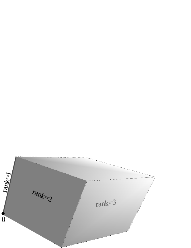
Figure 2: Schematic illustration of the topology of the subspaces of rank-$k$ matrices, $k=0,1,2,3$.

Example 2.4

Fix some bijection $\mathbb{N}\times\mathbb{N}\to\mathbb{N}$, $(x,y)\mapsto\langle x,y\rangle$; e.g. $\langle x,y\rangle:=2^{x}\cdot(1+2y)$.

1. For $\bar{n}\in\mathbb{N}^{*}$, let $\langle\bar{n}\rangle:=\sum_{i}2^{-\langle i,n_{i}\rangle}$; and map the empty tuple to 0.
   This mapping $\langle\,\cdot\,\rangle:\mathbb{N}^{*}\to[0,1]$ is injective and maps to dyadic rationals. For each $k\in\mathbb{N}$, the range $\langle\mathbb{N}^{k}\rangle$ belongs to $\Delta_{2}$; $\langle\mathbb{N}^{\leq k}\rangle$ is even closed a subset of $[0,1]$.

2. Consider $f:[0,1]\to[0,1]$ well-defined by $f(x):=1/k$ for $x=\langle\bar{n}\rangle$ with $\bar{n}\in\mathbb{N}^{k}$; $f(x):=0$ for $x\not\in\langle\mathbb{N}^{*}\rangle$. Then $f$ is $\Delta_{2}$-measurable but not $d$-continuous for any $d\in\mathbb{N}$.

Proof (Example 2.4)

1. Since the sum $\sum_{i\leq k}$ is finite for $\bar{n}\in\mathbb{N}^{k}$, $\langle\bar{n}\rangle$ amounts to a dyadic rational, namely one with at most $k$ occurrences of the digit 1; the latter constitute a closed set.

2. Well-definition of $f$ follows from a). Moreover, $f^{-1}(1/k)=\langle\mathbb{N}^{k}\rangle$ is in $\Delta_{2}$. Since $\operatorname{range}(f)=\{1/k:k\in\mathbb{N}\}\cup\{0\}$, the preimage $f^{-1}[V]$ of any open set $V\not\ni 0$ is a union of finitely many $f^{-1}(1/k)$ and therefore in $\Delta_{2}$, too; Whereas the preimage of open $V\ni 0$ misses finitely many $f^{-1}(1/k)$ and thus also belongs to $\Delta_{2}$.
   Let $x:=0$, $x_{n}:=2^{-\langle 1,n\rangle}$, $x_{n,m}:=2^{-\langle 1,n\rangle}+2^{-\langle 2,m\rangle}$, …, $x_{n_{1},\ldots,n_{d}}:=\sum_{i=1}^{d}2^{-\langle i,n_{i}\rangle}$. This constitutes a uniform $d$-dimensional flag. And $f(x_{n_{1},\ldots,n_{k}})=1/k\neq 1/(k+\ell)=f(x_{n_{1},\ldots,n_{k},\underbrace{\scriptstyle m,\ldots,m}_{\scriptscriptstyle\ell\text{ times}}})$ shows it to be a witness of $d$-discontinuity of $f$. ∎

Recall Example 1.4 of computing (or rather identifying) from a given $N$-tuple $(\vec{x}_{1},\ldots,\vec{x}_{N})$ of distinct points in $\mathbb{R}^{d}$ those extremal to (i.e. minimal and spanning) the convex hull $\operatorname{chull}(\vec{x}_{1},\ldots,\vec{x}_{N})$. In the 1D case, this problem $(x_{1},\ldots,x_{N})\mapsto\operatorname{extchull}_{N}(x_{1},\ldots,x_{N})$ is computable: simply return the two (distinct!) numbers $\min\{x_{1},\ldots,x_{N}\}$ and $\max\{x_{1},\ldots,x_{N}\}$. We have already seen that in 2D it generally lacks $\psi^{2}_{\!\raisebox{0.60275pt}{${\scriptscriptstyle>}$}}$–computability because of discontinuity.

Proposition 3

Let $\vec{x}_{1},\ldots,\vec{x}_{N}\in\mathbb{R}^{d}$ be pairwise distinct and $C:=\operatorname{chull}(\vec{x}_{1},\ldots,\vec{x}_{N})$.

1. Let $\vec{y}\in\operatorname{ext}(C)$. Then there exists a closed halfspace

   $$H^{+}_{\vec{u},t}\;=\;\big{\{}\vec{z}\in\mathbb{R}^{d}:\sum\nolimits_{i}z_{i}u_{i}\geq t\big{\}}\;\subseteq\;\mathbb{R}^{d}$$

   with rational normal (although not necessarily unit) vector $\vec{u}\in\mathbb{Q}^{d}\setminus\{0\}$ and $t>0$ such that $H^{+}\cap\{\vec{x}_{1},\ldots,\vec{x}_{N}\}=\{\vec{y}\}=\{\vec{x}_{j}\}$ for some $1\leq j\leq N$.

2. Conversely $H^{+}_{\vec{u},t}\cap\{\vec{x}_{1},\ldots,\vec{x}_{N}\}=\{\vec{x}_{j}\}$ with $\vec{u}\neq 0$ implies $\vec{x}_{j}\in\operatorname{ext}(C)$.

3. Given $\vec{x}_{1},\ldots,\vec{x}_{N}\in\mathbb{R}^{d}$ as above and for $1\leq j\leq N$, “$\vec{x}_{j}\in\operatorname{ext}(C)$” is semi-decidable.

4. The mapping $\operatorname{extchull}_{N}$ from Equation 2 is $(\rho^{d\times N},\psi^{d}_{\!\raisebox{0.60275pt}{${\scriptscriptstyle<}$}})$–computable.

5. For $N\geq 2$ and given the number $M:=\operatorname{Card}\operatorname{ext}(C)\in\{2,\ldots,N\}$ of extreme points, the set of their indices, i.e.

   $$\{i_{1},\ldots,i_{M}\}\subseteq\{1,\ldots,N\}\quad\text{s.t.}\quad\operatorname{ext}(C)=\{\vec{x}_{i_{1}},\ldots,\vec{x}_{i_{M}}\}$$

   becomes $(\rho^{d\times N},\nu)$–computable.
   In particular, $\operatorname{extchull}_{N}$ is $(\rho^{d\times N},\psi^{d}_{\!\raisebox{0.60275pt}{${\scriptscriptstyle>}$}})$–computable with $(N-1)$-wise advice.

6. It is however $(N-2)$-wise $(\rho^{d\times N},\psi^{d}_{\!\raisebox{0.60275pt}{${\scriptscriptstyle>}$}})$–discontinuous in dimensions $d\geq 2$.

Proof

1. Follows from c) by trying all $j=1,\ldots,N$. Indeed, a $\psi^{d}_{\!\raisebox{0.60275pt}{${\scriptscriptstyle<}$}}$–name (but not a $\psi^{d}_{\!\raisebox{0.60275pt}{${\scriptscriptstyle>}$}}$–name) permits to ‘increase’ at any time the set to be output.

2. similarly to d), now trying all $M$-tuples $(i_{1}<i_{2}<\cdots<i_{M})$ in $\{1,\ldots,N\}$. Note that indeed $\operatorname{Card}\operatorname{ext}(C)\geq 2$ because the $\vec{x}_{i}$ are pairwise distinct.

3. Follows from a+b) by dovetailed search for some $\vec{u}\in\mathbb{Q}^{d}\setminus\{0\}$ with $\langle\vec{u},\vec{x}_{j}\rangle=:t>\langle\vec{u},\vec{x}_{i}\rangle$ for all $i\neq j$, where $\langle\vec{u},\vec{x}\rangle:=u_{1}x_{1}+\cdots+u_{d}x_{d}$.

4. and b): It is well-known [Grue67] that extreme points $\vec{y}$ of a polytope $C$ (although not necessarily of a general convex body) are precisely its exposed points, i.e. satisfy $\{\vec{y}\}=C\cap H_{\vec{u},t}^{+}$ for some $t>0$ and $\vec{u}\in\mathbb{R}\setminus\{0\}$. Equivalently: $\langle\vec{u},\vec{x}_{j}\rangle>\langle\vec{u},\vec{x}_{i}\rangle$ for all $i\neq j$—obviously a condition open in $\vec{u}$, which therefore may be chosen from the dense subset $\mathbb{Q}^{d}\subseteq\mathbb{R}^{d}$.

5. We might construct a witness of $(N-2)$-discontinuity, but take the more elegant approach of a reduction by virtue of Lemma 1b). To this end observe that semi-decidability of inequality makes $\operatorname{Card}_{n}\mathbb{R}^{n}\ni(x_{1},\ldots,x_{n})\to\operatorname{Card}\{x_{1},\ldots,x_{n}\}$ $(\rho^{n},\rho_{\raisebox{0.60275pt}{${\scriptscriptstyle<}$}})$–computable, i.e. upper semi-continuous; hence by Example 2.2, $\operatorname{Card}_{n}$ must be $(n-1)$-wise lower semi-discontinuous.
   Now let $x_{1},\ldots,x_{n}\in\mathbb{R}$ be given. According to [Weih00, Exercise 4.3.15] suppose w.l.o.g. $x_{1}\geq x_{2}\geq\cdots\geq x_{n-1}\geq x_{n}=0$. Then proceed to the following collection $X$ of $(n+1)$ points in 2D: $(0,0)$, $(1,x_{1})$, $(2,x_{1}+x_{2})$, …, $(n-1,x_{1}+\cdots+x_{n-1})$, $(n,x_{n})$; cf. Figure 3. Let $f_{n}:\mathbb{R}^{n}\to\mathbb{R}^{2\times(n+1)}$ denote this computable mapping $(x_{1},\ldots,x_{n})\mapsto X$. Observe that the sequence of slopes from points $\#i$ to $\#i+1$ is non-increasing because $x_{i}\geq x_{i+1}$; and two successive slopes $(\#i-1\to\#i)$ and $(\#i\to\#i+1)$ coincide  iff  $x_{i}=x_{i+1}$; which in turn is equivalent to point $\#i$ not being extreme to $\operatorname{chull}(X)$. In fact from a $\psi^{2}_{\!\raisebox{0.60275pt}{${\scriptscriptstyle>}$}}$–name of $\operatorname{extchull}(X)$ one can semi-decide $(i,x_{1}+\cdots+x_{i})\not\in\operatorname{extchull}(X)$; cf. e.g. [Zieg04, Lemma 25c]. This yields a $(\psi^{2}_{\!\raisebox{0.60275pt}{${\scriptscriptstyle>}$}},\rho_{\raisebox{0.60275pt}{${\scriptscriptstyle>}$}})$–computable mapping $h_{n}:\operatorname{extchull}_{n+1}(X)\mapsto\operatorname{Card}\operatorname{extchull}_{n+1}(X)=\operatorname{Card}\{x_{1},\ldots,x_{n}\}$ defined on the image of $\operatorname{extchull}_{n+1}\circ f_{n}$. Now since $h_{n}\circ\operatorname{extchull}_{n+1}\circ f_{n}=\operatorname{Card}:\mathbb{R}^{n}\to\{1,\ldots,n\}$ is $(n-1)$-wise lower semi-discontinuous by the above considerations, Lemma 1b) requires that $\operatorname{extchull}_{n+1}$ be $(n-1)$-wise $(\rho^{n+1},\psi^{2}_{\!\raisebox{0.60275pt}{${\scriptscriptstyle>}$}})$–discontinuous. ∎

Figure 3: Knowing in 2D which points are/not extreme to their convex hull can be used to conclude which real numbers are in-/equal:

2.3 Further Remarks

For some time the author had felt that when $\operatorname{dom}(f)$ is sufficiently ‘nice’ and for $x\in\operatorname{dom}(f)$, the cardinal of discontinuity of $f$ could be lower bounded in terms of the number of distinct limits of $f$ at $x$, that is the cardinality of

$$\operatorname{Lim}(f,x)\quad:=\quad\big{\{}\lim\nolimits_{n\to\infty}f(x_{n}):\operatorname{dom}(f)\ni x_{n}\to x\big{\}}\enspace.$$

However the following example (cf. also the right part of Figure 4) shows that this is not the case:

$$f:[-1,1]\to[0,1],\qquad 2^{-n}\cdot 3^{-m}\mapsto 3^{-m}\quad(n,m\in\mathbb{N}),\qquad f(x):\equiv 0\text{ otherwise}\enspace.$$

Here $\operatorname{Lim}(f,0)$ is infinite but $f$ is continuous on $D_{1}:=\{2^{-n}\cdot 3^{-m}:n,m\in\mathbb{N}\}$ (because the latter set contains no accumulation point) and $f\equiv 0$ on $D_{2}:=[-1,1]\setminus D_{1}$; hence $\mathfrak{C}_{\rm t}(f)=2$.

  

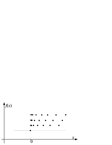
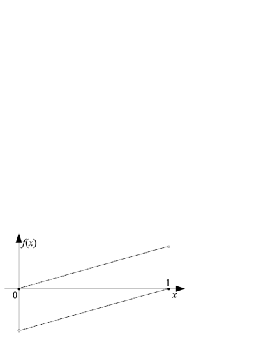
Figure 4: Left: the cardinal of discontinuity cannot be lower bounded by the number of limit points. Right: A 2-continuous function which, after identifying arguments $x=0$ and $x=1$, exhibits mere 3-continuity.

In order to apply Lemma 2 for proving $k$-discontinuity of a function $f:A\to B$, it may help to compactify the co-domain:

Example 2.5

Consider $f:[0,1]\to\mathbb{R}$, $0\mapsto 0$, $0<x\mapsto 1/x$.
Then $f$ admits no witness of 1-discontinuity;
whereas $\tilde{f}:[0,1]\to\mathbb{R}\cup\{+\infty\}$ does admit such a witness.

The crucial point is of course that $x:=0$ and $x_{n}:=1/n$ constitutes a witness of 1-discontinuity only for $\tilde{f}$, because $0=f(x)\neq\lim_{n}f(x_{n})=+\infty$ exists only in $\mathbb{R}\cup\{+\infty\}$. Finally we remark that the notation $\delta$ in Definition 1b) is usually straight-forward and natural; although an artificially bad choice is possible even for $2$-wise computable functions:

Example 2.6

The characteristic function $\chi_{H}:\mathbb{N}\to\{0,1\}$ of the Halting problem $H\subseteq\mathbb{N}$ is obviously 2-wise $(\nu,\nu)$–computable by virtue of $\Delta=\{H,\mathbb{N}\setminus H\}$, namely for $\delta:\subseteq\Sigma^{*}\to\Delta$ with $1\mapsto H$ and $0\mapsto\mathbb{N}\setminus H$.
Whereas with respect to the following notation $\tilde{\delta}$, $\chi_{H}$ is equally obviously not $(\nu,\tilde{\delta},\nu)$–computable:

$$\delta:\Sigma^{*}\to\Delta,\qquad\bar{x}\mapsto H\text{ for }\bar{x}\in H,\quad\bar{x}\mapsto\mathbb{N}\setminus H\text{ for }\bar{x}\not\in H\enspace.$$

2.4 Weak $k$-wise Advice

Recalling Observation 1.5, (weak) $k$-wise $(\alpha,\beta)$-computability of $f:\subseteq A\to B$ implies (weak) $k$-wise $(\alpha,\beta)$-continuity from which in turn follows weak $k$-wise $(\alpha,\beta)$-continuity in the following sense:

Definition 4

Consider a function $f:A\to B$ between represented spaces $(A,\alpha)$ and $(B,\beta)$.

1. Call $f$ $k$-wise $(\alpha,\beta)$-continuous if there exists a partition $\Delta$ of $\operatorname{dom}(f)$ of $\operatorname{Card}(\Delta)=k$ such that $f|_{D}$ is $(\alpha,\beta)$-continuous on each $D\in\Delta$.

2. Call $f$ weakly $k$-wise $(\alpha,\beta)$-continuous if there exists a $k$-continuous $(\alpha,\beta)$-realizer $F:\subseteq\Sigma^{\omega}\to\Sigma^{\omega}$ of $f$ in the sense of [Weih00, Definition 3.1.3].

3. Call $f$ weakly $k$-wise $(\alpha,\beta)$-computable if it admits a $k$-computable $(\alpha,\beta)$-realizer.

However conversely, and as opposed to the classical case $k=1$, weak $2$-wise $(\alpha,\beta)$–continuity in generally does not imply $2$-wise $(\alpha,\beta)$-continuity. Basically the reason is that a partition of $\operatorname{dom}(f)$ yields a partition of $\operatorname{dom}(F)$; whereas a partition $\Delta$ of $\operatorname{dom}(F)$ need not be compatible with the representation in that different $\alpha$ names for the same argument $a$ may belong to different elements of $\Delta$:

Example 2.7

Consider the following function depicted to the right of Figure 4

$$f:[0,1]\to[-1,+1],\qquad[0,1)\cap\mathbb{Q}\ni x\mapsto x=:g(x),\quad\mathbb{R}\setminus\mathbb{Q}\ni x\mapsto x-1=:h(x),\quad f(1):=0.$$

It is continuous on both $\mathbb{Q}\cap[0,1)$ and on $\{1\}\cup\mathbb{R}\setminus\mathbb{Q}$; hence 2-continuous, and admits a 2-continuous $(\rho,\rho)$–realizer.

Now proceed from $[0,1]$ to $\mathcal{S}^{1}$, i.e. identify $x=0$ with $x=1$; formally, consider the representation $\tilde{\rho}:=\imath\circ\rho:\subseteq\Sigma^{\omega}\to\mathcal{S}^{1}$ where $\imath:\mathbb{R}\to[0,1)$, $x\mapsto x\mod 1$. Since $f(0)=0=f(1)$, this induces a well-defined function $\tilde{f}:\mathcal{S}^{1}\to[-1,+1]$; which admits a 2-continuous $(\tilde{\rho},\rho)$–realizer: namely the 2-continuous $(\rho,\rho)$–realizer of $f$. But $\tilde{f}$ itself is not 2-continuous:
Suppose $\mathcal{S}^{1}=D_{1}\uplus D_{2}$ where $\tilde{f}|_{D_{1}}$ and $\tilde{f}|_{D_{2}}$ are both continuous. W.l.o.g. $0\in D_{1}$. Observe that $\tilde{f}(0)=0=g(0)\neq h(0)=-1$. Hence, as $\mathbb{Q}$ is dense and because continuous $h$ is different from continuous $g$, continuity of $\tilde{f}|_{D_{1}}$ requires it to coincide with $g$: first just locally at $x=0$, but then also globally—which implies $\lim\limits_{x\nearrow 1}\tilde{f}|_{D_{1}}(x)=g(1)=1$, contradicting $\tilde{f}|_{D_{1}}(1)=0$. ∎

As already mentioned, Example 2.7 illustrates that the implication from $k$-wise $(\alpha,\beta)$-continuity to weak $k$-wise $(\alpha,\beta)$-continuity cannot be reversed in general—even for admissible representations. Indeed, $\tilde{\rho}$ can be shown equivalent to the standard representation $\delta_{\mathcal{S}^{1}}$ of $\mathcal{S}^{1}$ as an effective topological space [Weih00, Definition 3.2.2].

Applying Lemma 1 to realizers yields the following counterpart for weak advice:

Remark 2.8

Fix represented spaces $(A,\alpha)$, $(B,\beta)$, and $(C,\gamma)$.

1. Let $f:A\to B$ be weakly $d$-wise $(\alpha,\beta)$-continuous/computable and $A^{\prime}\subseteq A$. Then the restriction $f|_{A^{\prime}}$ is again weakly $d$-wise $(\alpha,\beta)$-continuous/computable.

2. Let $f:A\to B$ be weakly $d$-wise $(\alpha,\beta)$-continuous/computable and $g:B\to C$ be weakly $k$-wise $(\beta,\gamma)$-continuous/computable. Then $g\circ f:A\to C$ is weakly $d\cdot k$-wise $(\alpha,\gamma)$-continuous/computable.

3. If $f:A\to B$ is weakly $d$-wise $(\alpha,\beta)$-continuous (computable) and $\alpha^{\prime}\preceq_{\rm t}\alpha$ ($\alpha^{\prime}\preceq\alpha$) and $\beta\preceq_{\rm t}\beta^{\prime}$ ($\beta\preceq\beta^{\prime})$, then $f$ is also weakly $d$-wise $(\alpha^{\prime},\beta^{\prime})$–continuous (computable).

Notice that property b) does not carry over to multi-representations in the sense of [Weih08]; cf. the discussion preceeding Lemma 3 below.

We also observe that Lemma 2 does not admit a converse, even for total functions between compact spaces:

Observation 2.9

The function $\tilde{f}:\mathcal{S}^{1}\to[-1,+1]$ from Example 2.7 is not 2-continuous yet has no witness of 2-discontinuity.

Proof

Suppose $\big{\{}x,(x_{n}),(x_{n,m})\big{\}}$ is a witness of 2-discontinuity of $\tilde{f}$. First consider the

• case $x\in(0,1)\cap\mathbb{Q}$. Since $x_{n}\to x$ and $x=\tilde{f}(x)\neq\lim_{n}\tilde{f}(x_{n})$, w.l.o.g. $0<x_{n}<1$ and $x_{n}\not\in\mathbb{Q}$: otherwise proceed to an appropriate subsequence. Now $\lim_{m}x_{n,m}=x_{n}$ and $\lim_{m}\tilde{f}(x_{n,m})\neq\tilde{f}(x_{n})=x_{n}-1$ requires, by definition of $\tilde{f}$, $\tilde{f}(x_{n,m})=x_{n,m}$ for almost all $m$ and $n$: contradicting that a witness of discontinuity is required to satisfy $\lim_{m}\tilde{f}(x_{m,m})\neq\tilde{f}(x)$ and $\lim_{m}x_{m,m}=x$.

• Case $x\in(0,1)\setminus\mathbb{Q}$: similarly.

• Case $x=0\equiv 1$: As $x_{n}\to x$ and since $0\neq\tilde{f}(x)\neq\lim_{n}\tilde{f}(x_{n})$ exists, we may consider two subcases:

• Subcase $x_{n}\in(1/2,1)\cap\mathbb{Q}$ for almost all $n$:
  Now $x_{n}=\lim_{m}x_{n,m}$ and $x_{n}=\tilde{f}(x_{n})\neq\lim_{m}\tilde{f}(x_{n,m})$ requires, by definition of $\tilde{f}$, $\tilde{f}(x_{n,m})=x_{n,m}-1$ for almost all $m$ and $n$: contradicting $\lim_{m}x_{m,m}=x$ and $\lim_{m}\tilde{f}(x_{m,m})\neq\tilde{f}(x)=0$.

• Subcase $x_{n}\in(0,1/2)\setminus\mathbb{Q}$ for almost all $n$: similarly. ∎

3 Multivalued Functions, i.e. Relations

Many applications involve functions which are ‘non-deterministic’ in the sense that, for a given input argument $x$, several values $y$ are acceptable as output; recall e.g. Items i) and ii) in Section 1. Also in linear algebra, given a singular matrix $A$, we want to find some (say normed) vector $\vec{v}$ such that $A\cdot\vec{v}=0$. This is reflected by relaxing the mapping $f:x\to y$ to be not a function but a relation (also called multivalued function); writing $f:X\rightrightarrows Y$ instead of $f:X\to 2^{Y}\setminus\{\emptyset\}$ to indicate that for an input $x\in X$, any output $y\in f(x)$ is acceptable. Many practical problems have been shown computable as multivalued functions but admit no computable single-valued so-called selection; cf. e.g. [Weih00, Exercise 5.1.13], [ZiBr04, Lemma 12 or Proposition 17], and the left of Figure 5 below. On the other hand, even relations often lack computability merely for reasons of continuity—and appropriate additional discrete advice renders them computable, recall Example 1.2 above.

Now Definition 1 of the complexity of non-uniform computability straight-forwardly extends from single-valued to multivalued functions; and Observation 1.5 relates them to (single-valued) realizers; which can then be treated using Lemma 2. However a direct generalization of Lemma 2 to multivalued mappings turns out to be more convenient. This approach requires a notion of (dis-)continuity for relations rather than for functions.

3.1 Continuity for Multivalued Mappings

Like single-valued computable functions (recall the Main Theorem), also computable relations satisfy certain topological conditions. However for such multivalued mappings, literature knows a variety of easily confusable notions [ScNe07]. Hemicontinuity for instance is not necessary for real computability; cf. Example 3.1a) below. It may be tempting to regard computing a multivalued mapping $f$ as the task of calculating, given $x$, the set-value $f(x)$ [Spre08]. In our example applications, however, one wants to capture that a machine is permitted, given $x$, to ‘nondeterministically’ choose and output some value $y\in f(x)$. Note that this coincides with [Weih00, Definition 3.1.3]. In particular we do not insist that, upon input $x$, all $y\in f(x)$ occur as output for some nondeterministic choice—as required in [Brat03, Section 7]. Instead, let us generalize Definition 3 as follows:

Definition 5

Fix some possibly multivalued mapping $f:\subseteq X\rightrightarrows Y$ and write $\operatorname{dom}(f):=\{x\in X:f(x)\neq\emptyset\}$.
Call $f$ continuous at $x\in X$ if there is some $y\in f(x)$ such that for every open neighbourhood $V$ of $y$ there exists a neighbourhood $U$ of $x$ such that $f(z)\cap V\neq\emptyset$ for all $z\in U$.

For ordinary (i.e. single-valued) functions $f$, $\operatorname{dom}(f)$ amounts to the usual notion; and such $f$ is obviously continuous (at $x$) iff it is continuous (at $x$) in the original sense.

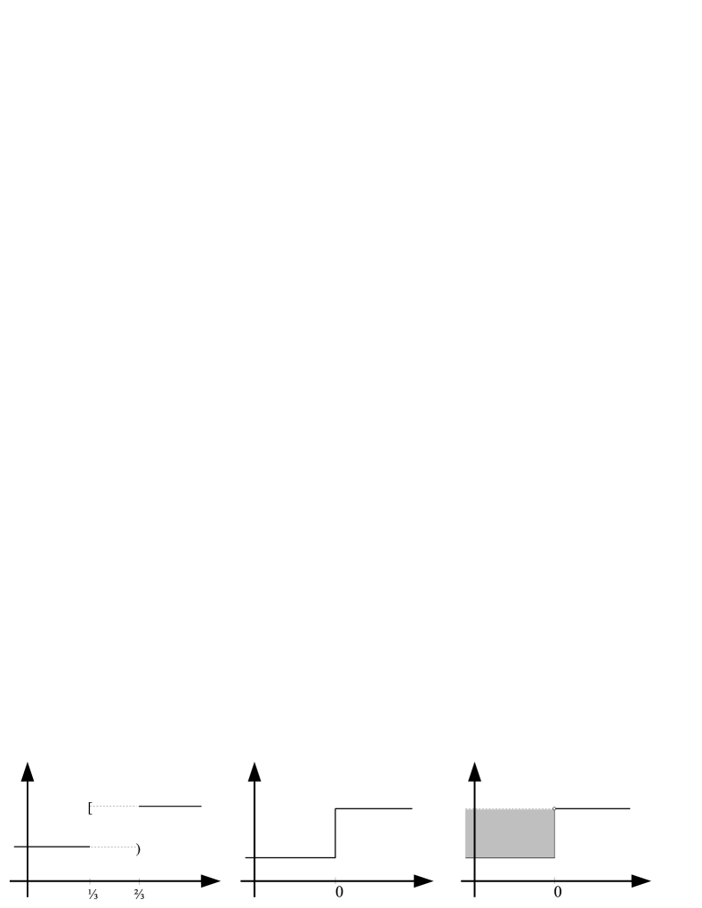
Figure 5: Left: A $(\rho,\rho)$–computable relation which is not hemicontinuous nor admits a continuous selection. Middle: Quantification over all $y\in f(x)$ is generally necessary to capture discontinuity of a multivalued function.

Example 3.1

1. Consider the left of Figure 5, i.e. the multivalued function

   $$f:[0,1]\rightrightarrows[0,1],\qquad 1/3>x\mapsto\{0\},\quad[1/3,2/3)\ni x\mapsto\{0,1\},\quad 2/3\leq x\mapsto\{1\}\enspace.$$

   Then $f$ is neither lower nor upper hemicontinuous—yet $(\rho,\rho)$–continuous, even computable: Given $(q_{n})\subseteq\mathbb{Q}$ with $|x-q_{n}|\leq 2^{-n}$, test $q_{3}$: if $q_{3}\leq 1/2$ output $0$, otherwise output $1$. Indeed, $|x-q_{3}|\leq 1/8$ implies $x\leq 5/8<2/3$ for $q_{3}\leq 1/2$, hence $0\in f(x)$; whereas $q_{3}>1/2$ implies $x\geq 3/8>1/3$, hence $1\in f(x)$.

2. Referring to the middle part of Figure 5, the multivalued function

   $$g:[-1,1]\rightrightarrows[0,1],\qquad[-1,0)\ni x\mapsto\{0\},\quad 0\mapsto[0,1],\quad(0,1]\ni x\mapsto\{1\}$$

   is not continuous at 0 w.r.t. any $y\in f(0)=[0,1]$ although $f(0)$ itself does intersect $f(z)$ for all $z$.

3. Consider the right part of Figure 5, i.e. the multivalued function

   $$h:[-1,+1]\rightrightarrows[0,1],\qquad 0\geq x\mapsto[0,1),\quad 0<x\mapsto\{1\}\enspace.$$

   Then $x_{n}:=2^{-n}$ constitutes a witness of discontinuity of $h$ at $x=0$ in the sense of Definition 6a) below: For every $y\in h(x)=[0,1)$, $V:=(0,y/2+1/2)\ni y$ is an open neighbourhood of $y$ disjoint from $h(x_{n})=\{1\}$ for all $n$.

Lemma 1a) literally applies also to multivalued mappings $f:A\rightrightarrows B$. Similarly generalizing Lemma 1b) is quite cumbersome: For $B=\bigcup_{i}B_{i}$, the preimages $f^{-1}[B_{i}]$,

• if defined as $\{a\in A:f(a)\subseteq B_{i}\}$, need not cover $A$

• if defined as $\{a\in A:f(a)\cap B_{i}\neq\emptyset\}$, need not be mapped to within $B_{i}$ by $f$.

On the other hand, already the following partial generalization of Lemma 1b) turns out as useful:

Lemma 3

1. Let $f:A\to B$ be single-valued and $g:B\rightrightarrows C$ multivalued. If $f$ is $d$-continuous (computable) and $g$ is $k$-continuous (computable), then $g\circ f:A\rightrightarrows C$ is $(d\cdot k)$-continuous (computable).

2. Let $f:A\rightrightarrows B$ and $g:B\rightrightarrows C$ be multivalued. If $f$ is $d$-continuous (computable) and $g$ is continuous (computable), then $g\circ f:A\rightrightarrows C$ is again $d$-continuous (computable).

Proof

1. Since $f$ is single-valued, the set $A_{i}\cap f^{-1}[B_{j}]$ is unambiguous and mapped by $f$ to a subset of $B_{j}$; that is the proof of Lemma 1b) carries over.

2. If $f$ is continuous (computable) on each $A_{i}$, then so is $g\circ f$. ∎

Lemma 4a) below is an immediate extension of the Main Theorem of Recursive Analysis, showing that any computable multivalued mapping is necessarily continuous. It seems unknown whether also the converse, namely the Kreitz-Weihrauch Representation Theorem, extends to the multivalued (for a start, real) case:

Question 3.2

Is the notion of multivalued continuity in Definition 5 strong enough to assert that any function $f:\subseteq\mathbb{R}\rightrightarrows\mathbb{R}$ satisfying it admits a Cantor-continuous $(\rho,\rho)$–realizer?

3.2 Witnesses of Discontinuity

Definition 6

1. For $x\in\operatorname{dom}(f)$, a witness of discontinuity of $f$ at $x$ is a sequence $(x_{n})\in\operatorname{dom}(f)$ converging to $x$ such that, for every $y\in f(x)$ there is some open neighbourhood $V$ of $y$ disjoint from $f(x_{n})$ for infinitely many $n\in\mathbb{N}$.

2. A uniform $d$-dimensional flag $\mathcal{F}$ in $X$ is a witness of $d$-discontinuity of $f$ if, for each $0\leq k<d$ and for each $\bar{n}\in\mathbb{N}^{k}$ and for each $1\leq\ell\leq d-k$ and for each $y\in f(x_{\bar{n}})$, $\big{(}x_{\bar{n},\underbrace{\scriptscriptstyle m,\ldots,m}_{\ell\text{ times}}}\big{)}_{m}$ is a witness of discontinuity of $f$ at $x_{\bar{n}}$.

If multivalued $f$ admits a witness of discontinuity at $x$, then $f$ is not continuous. Conversely, if $X$ is first-countable, discontinuity of $f$ at $x$ yields the existence of a witness of discontinuity at $x$. Also, witnesses of $1$-discontinuity coincide with witnesses of discontinuity; and they generalize the definition from the single-valued case. Lemma 4 below extends Lemma 2 in showing that a witness of $d$-discontinuity of $f$ inhibits $d$-computability.

Lemma 4

Let $(A,\alpha)$ and $(B,\beta)$ be effective metric spaces with corresponding Cauchy representations and $f:\subseteq A\rightrightarrows B$ a possibly multivalued mapping.

1. If $f$ admits a witness of discontinuity, then it is not $(\alpha,\beta)$–continuous.

2. If $f$ admits a witness of $d$-discontinuity, then it is not $d$-wise $(\alpha,\beta)$–continuous.

Proof

1. Suppose $F:\subseteq\Sigma^{\omega}\to\Sigma^{\omega}$ is a continuous $(\alpha,\beta)$–realizer of $f$. It maps some $\alpha$-name $\bar{\sigma}$ of $x$ to a $\beta$-name $\bar{\tau}$ of some $y\in f(x)$. Now consider the neighbourhood $V\ni y$ according to Definition 5b). By definition of the Cauchy representation $\beta$, some finite initial part $(\tau_{1},\ldots,\tau_{M})=:\bar{\tau}|_{\leq M}$ of $\bar{\tau}$ restricts $y$ to belong to $V$; and by continuity of $F$, this $\bar{\tau}|_{\leq M}$ depends on some finite initial part $\bar{\sigma}|_{\leq N}$ of $\bar{\sigma}$. On the other hand $\bar{\sigma}|_{\leq N}$ is also initial part of an $\alpha$-name of some element $x_{n}$ of the witness of discontinuity; in fact of infinitely many of them. But for $n$ sufficiently large, $f(x_{n})$ was supposed to not meet $V$; that is $\bar{\tau}|_{\leq M}$ is not initial part of a $\beta$-name of any $y^{\prime}\in f(x_{n})$: contradiction.

2. combines the arguments for a) with the proof of 2. ∎

In comparison with the single-valued case, a witness of discontinuity of a multivalued mapping involves one additional quantifier ranging universally over all $y\in f(x)$; and Example 3.1b) shows that this is generally also necessary. Nevertheless, the following tool gives a (weaker yet) simpler condition to be applied in Section 4.

Lemma 5

Fix metric spaces $(A,\alpha)$ and $(B,\beta)$, $\epsilon>0$, and $f:\subseteq A\rightrightarrows B$.

1. For $S,T\subseteq A$, $B(S,\epsilon):=\{a\in A|\exists s\in S:d_{A}(a,s)<\epsilon\}$ is disjoint from $T$  iff  $B(T,\epsilon)$ is disjoint from $S$, and implies $B(S,\epsilon/2)\cap B(T,\epsilon/2)=\emptyset$.

2. Let $u_{n}$ and $v_{n}$ denote sequences in $\operatorname{dom}(f)$ with $\lim_{n}u_{n}=x=\lim_{n}v_{n}$ such that $B\big{(}f(u_{n}),\epsilon\big{)}$ is disjoint from $f(v_{n})$ for all but finitely many $n$. Then at least one of the sequences is a witness of discontinuity of $f$ at $x$.

3. For $r\in\mathbb{N}$ and $1\leq i\leq r$, let $(x_{n}^{(i)})_{{}_{n}}$ denote sequences in $\operatorname{dom}(f)$ with $\lim_{n}x_{n}^{(i)}=x$ such that $\bigcap_{i=1}^{r}B\big{(}f(x_{n}^{(i)}),\epsilon\big{)}=\emptyset$ holds for infinitely many $n$. Then, for some $i$, $(x_{n}^{(i)})_{{}_{n}}$ is a witness of discontinuity of $f$ at $x$.

4. Fix $r,d\in\mathbb{N}$ and consider a family of (multi-)sequences

   $$x,\quad x_{n_{1}}^{(i_{1})},\quad x_{n_{1},n_{2}}^{(i_{1},i_{2})},\quad\ldots,\quad x_{n_{1},\ldots,n_{d}}^{(i_{1},\ldots,i_{d})},\qquad n_{1},\ldots,n_{d}\in\mathbb{N},\quad 1\leq i_{1},\ldots,i_{d}\leq r$$

   such that, for each $\bar{\imath}\in\{1,\ldots,r\}^{d}$, $\big{(}x,x_{n_{1}}^{(i_{1})},x_{n_{1},n_{2}}^{(i_{1},i_{2})},\ldots,x_{n_{1},\ldots,n_{d}}^{(i_{1},\ldots,i_{d})}\big{)}$ constitutes a uniform $d$-dimensional flag. Furthermore suppose that, for each $\bar{n}\in\mathbb{N}^{k}$ and $\bar{\imath}\in\{1,\ldots,r\}^{k}$ ($0\leq k<d$) and for each $1\leq\ell\leq d-k$,

   $$\bigcap\nolimits_{j=1}^{r}B\Big{(}f\big{(}x^{(\bar{\imath},\overbrace{\scriptscriptstyle j,\ldots,j}^{\ell\text{ times}})}_{\bar{n},\underbrace{\scriptscriptstyle m,\ldots,m}_{\ell\text{ times}}}\big{)},\epsilon\Big{)}\quad=\quad\emptyset$$ (3)

   for infinitely many $m\in\mathbb{N}$. Then this family contains a witness of $d$-discontinuity of $f$.

Proof

1. If $t\in T\cap B(S,\epsilon)$, there is some $s\in S$ with $d_{A}(s,t)<\epsilon$; hence $s\in S\cap B(T,\epsilon)$. So $T\cap B(S,\epsilon)\neq\emptyset$ implies $S\cap B(T,\epsilon)\neq\emptyset$. The converse implication holds symmetrically.
   For $x\in B(S,\epsilon/2)\cap B(T,\epsilon/2)$ there exist $s\in S$ and $t\in T$ with $d(s,x),d(t,x)<\epsilon/2$; hence $d(s,t)<\epsilon$ by triangle inequality and $s\in S\cap B(T,\epsilon)$.

2. Suppose conversely that there exists some $y\in f(x)$ such that $V:=B(y,\epsilon/2)$ intersects both $f(u_{n})$ and $f(v_{n})$ for all $n\geq n_{0}$. Then $y\in B(\big{(}f(u_{n}),\epsilon/2\big{)}\cap\big{(}f(v_{n}),\epsilon\big{)}$; hence by a), $B\big{(}f(u_{n}),\epsilon\big{)}$ intersects $f(v_{n})$: contradiction.

3. similarly.

4. The case $r=1$ is that of c). We now treat $r=2$, the cases of higher values proceed similarly.
   By c) there is some $i$ such that $\big{(}x_{n}^{(i)}\big{)}$ constitutes a witness of discontinuity of $f$ at $x$. Now consider the sequences $\big{(}x_{n,m}^{(i,j)}\big{)}_{{}_{m}}$ for $n\in\mathbb{N}$ and $1\leq j\leq r$. Again by c), to each $n$ there is some $j(n)\in\{1,\ldots,r\}$ such that $\big{(}x_{n,m}^{(i,j)}\big{)}_{{}_{m}}$ is a witness of discontinuity of $f$ at $x_{n}^{(i)}$. According to pigeonhole, $j(n)=j$ for some $j$ and for infinitely many $n$; hence we may proceed to an appropriate subsequence of $x_{n}$ and presume that $\big{(}x_{n,m}^{(i,j)}\big{)}_{{}_{m}}$ is a witness of discontinuity of $f$ at $x_{n}^{(i)}$ for one common $j$; and $\big{(}x_{m,m}^{(i,j)}\big{)}_{{}_{m}}$ a witness of discontinuity of $f$ at $x$: arriving at $\big{(}x,x^{(i)}_{n},x^{(i,j)}_{n,m}\big{)}$ a witness of 2-discontinuity of $f$. ∎

3.3 Example: Rational Approximations vs. Binary Expansion

It is long known [Turi37] that a sequence of rational approximations to some $x\in\mathbb{R}$ with error bounds cannot continuously be converted into a binary expansion of $x$. On the other hand for non-dyadic reals, i.e. for

$$x\;\not\in\;\mathbb{D}\;:=\;\big{\{}(2r+1)/2^{k}:r,k\in\mathbb{Z}\big{\}}\enspace,$$

such a conversion is computably possible [Weih00, Theorem 4.1.13.1]; while each rational $x=r/s$ has an (ultimately periodic, hence) computable binary expansion [Weih00, Theorem 4.1.13.2]. We observe that finding such an expansion for dyadic $x$ is infinitely discontinuous. Recall that $\tfrac{1}{2}=(0.1000\ldots)_{2}=(0.01111\ldots)_{2}$ (and in fact each $x\in\mathbb{D}$) admits two distinct binary expansions.

Proposition 4

The multivalued mapping

$$\operatorname{Adic}_{2}:\mathbb{D}\cap[0,1)\rightrightarrows\{0,1\}^{\omega},\quad\sum_{m=1}^{\infty}b_{m}2^{-m}\mapsto(b_{1},b_{2},\ldots)$$

is not $d$-wise $(\rho,\nu^{\omega})$-continuous for any $d\in\mathbb{N}$.

We remark that in fact for each $q=2,3,4,\ldots$, the mapping $\operatorname{Adic}_{q}$ extracting $q$-adic expansions is infinitely discontinuous on $\mathbb{Q}$.

Proof (Proposition 4)

Start with the rational sequence $q^{()}:=(\tfrac{1}{2},\tfrac{1}{2},\ldots)$, a $\rho$–name of $x:=\tfrac{1}{2}$. Then consider the sequence of sequences

$$q^{(+)}_{n}\;\;:=\;\;\big{(}\underbrace{\tfrac{1}{2},\ldots,\tfrac{1}{2}}_{n\text{ times}},\underbrace{\tfrac{1}{2}+2^{-n},\tfrac{1}{2}+2^{-n},\ldots}_{\infty\text{ times}}\big{)}\enspace:$$

$\rho$–names of $x^{(+)}_{n}:=\tfrac{1}{2}+2^{-n}$, since $|x^{(+)}_{n}-q^{(0)}_{n,\ell}|=2^{-n}\leq 2^{-\ell}$ for $\ell\leq n$. Moreover, $q^{(+)}_{n}$ converges in the Baire metric to the sequence $q^{()}$. Similarly, $q^{(-)}_{n}:=(\tfrac{1}{2},\ldots,\tfrac{1}{2},\tfrac{1}{2}-2^{-n},\tfrac{1}{2}-2^{-n},\ldots)$ is a $\rho$–name of $x^{(-)}:=\tfrac{1}{2}-2^{-n}$ also converging to $q^{()}$. And although the binary expansions of $x^{(+)}_{n}\neq x^{(-)}_{n}$ are both not unique,

$$x^{(+)}_{n} \;=\;(0.1\underbrace{0\cdots 0}_{\makebox[0.0pt]{$\scriptscriptstyle(n-2)\text{ times}$}}100\ldots)_{2}\;=\;(0.1\underbrace{0\cdots 0}_{\makebox[0.0pt]{$\scriptscriptstyle(n-2)\text{ times}$}}011\ldots)_{2}$$

$$x^{(-)}_{n} \;=\;(0.0\underbrace{1\cdots 1}_{\makebox[0.0pt]{$\scriptscriptstyle(n-2)\text{ times}$}}100\ldots)_{2}\;=\;(0.0\underbrace{1\cdots 1}_{\makebox[0.0pt]{$\scriptscriptstyle(n-2)\text{ times}$}}011\ldots)_{2}$$

shows that for $n\geq 2$ they must differ already in the first place. Put differently, for $\epsilon:=1/2$ and with respect to Cantor metric, $B\big{(}\operatorname{Adic}_{2}(x^{(+)}_{n}),\epsilon\big{)}\cap B\big{(}\operatorname{Adic}_{2}(x^{(-)}_{n}),\epsilon\big{)}=\emptyset$: a witness of discontinuity according to Lemma 4b).
Next take

$$q^{(\pm,\pm)}_{n,m}\;\;:=\;\;\big{(}\underbrace{\tfrac{1}{2},\ldots,\tfrac{1}{2}}_{n\text{ times}},\underbrace{\tfrac{1}{2}\pm 2^{-n},\ldots,\tfrac{1}{2}\pm 2^{-n}}_{m\text{ times}},\underbrace{\tfrac{1}{2}\pm 2^{-n}\pm 2^{-n-m},1/2\pm 2^{-n}\pm 2^{-n-m},\ldots}_{\infty\text{ times}}\big{)}$$

as $\rho$–names of $x^{(\pm,\pm)}_{n,m}:=\tfrac{1}{2}\pm 2^{-n}\pm 2^{-n-m}\not\in\{x,x^{(\pm)}_{n}:n\in\mathbb{N}\}$ converging to $q^{(\pm)}_{n}$ for $m\to\infty$; and $q^{(\pm,\pm)}_{m,m}$ to $q^{()}$. Here, any binary expansions of $x^{(s,-)}$ and of $x^{(s,+)}$ must differ in position $n$, i.e $B\big{(}\operatorname{Adic}_{2}(x^{(s,+)}_{n,m}),\epsilon\big{)}\cap B\big{(}\operatorname{Adic}_{2}(x^{(s,-)}_{n,m}),\epsilon\big{)}=\emptyset$ for $\epsilon\leq 2^{-n}$; while still $B\big{(}\operatorname{Adic}_{2}(x^{(+,s)}_{n,m}),\epsilon\big{)}\cap B\big{(}\operatorname{Adic}_{2}(x^{(-,s)}_{n,m}),\epsilon\big{)}=\emptyset$ for $\epsilon\leq 1/2$: yielding a witness of 2-discontinuity according to Lemma 4d) with $r:=2$.
And, continuing, $\displaystyle q^{(\pm,\ldots,\pm)}_{n_{1},\ldots,n_{d}}:=$

$$\Big{(} \underbrace{\tfrac{1}{2},\ldots,\tfrac{1}{2}}_{n_{1}\text{ times}},\underbrace{\tfrac{1}{2}\pm 2^{-n_{1}},\ldots,\tfrac{1}{2}\pm 2^{-n_{1}}}_{n_{2}\text{ times}},\underbrace{\tfrac{1}{2}\pm 2^{-n_{1}}\pm 2^{-n_{1}-n_{2}},\ldots,\tfrac{1}{2}\pm 2^{-n_{1}}\pm 2^{-n_{1}-n_{2}}}_{n_{3}\text{ times}},\ldots,$$

$$\ldots,\quad\ldots,\quad\ldots,$$

$$\underbrace{\tfrac{1}{2}\pm 2^{-n_{1}}\pm 2^{-n_{1}-n_{2}}\pm\cdots\pm 2^{-n_{1}-\cdots-n_{d-1}},\ldots,\tfrac{1}{2}\pm 2^{-n_{1}}\pm 2^{-n_{1}-n_{2}}\pm\cdots\pm 2^{-n_{1}-\cdots-n_{d-1}}}_{n_{d}\text{ times}},$$

$$\underbrace{\tfrac{1}{2}\pm 2^{-n_{1}}\pm 2^{-n_{1}-n_{2}}\pm\cdots\pm 2^{-n_{1}-\cdots-n_{d-1}}\pm 2^{-n_{1}-\cdots-n_{d-1}-n_{d}},\ldots}_{\infty\text{ times}}\Big{)}$$

constitutes a compact $d$-flag of $\rho$–names for $x^{(\pm,\ldots,\pm)}_{n_{1},\ldots,n_{d}}:=1/2\pm 2^{-n_{1}}\pm 2^{-n_{1}-n_{2}}\pm\cdots\pm 2^{-n_{1}-\cdots-n_{d-1}}$ and witness of $d$-discontinuity of $\operatorname{Adic}_{2}$. ∎

Now consider the problem $\operatorname{Adic}_{2}^{(n)}:[0,1)\rightrightarrows\{0,1\}^{n}$ of computing only the first $n$ bits of the binary expansion of $x$, given by rational approximations with error bounds. Since $\operatorname{Adic}_{2}(x)$ is in a sense the limit of $\operatorname{Adic}_{2}^{(n)}(x)$ converging with $2^{-n}$ as $n\to\infty$, it might seem natural to conjecture in view of Proposition 4 that $\mathfrak{C}_{\rm c}(\operatorname{Adic}_{2}^{(n)},\rho,\nu)\to\infty$ for $n\to\infty$. Indeed $2^{n}$-wise advice trivially suffices for computing $\operatorname{Adic}_{2}^{(n)}(x)\in\{0,1\}^{n}$. But one can do much better:

Observation 3.3

$\operatorname{Adic}_{2}^{(n)}:[0,1)\rightrightarrows\{0,1\}^{n}$ is $(\rho,\nu)$–computable with 2-wise advice; namely when giving, in addition to a $\rho$–name of $x$, also the $n$-th bit of its binary expansion.

This can be considered an example of a phase transition. (Note however that, implicitly, $n$ is given here.)

Proof (Observation 3.3)

Suppose that $[0,1)\ni x=\sum_{i=1}^{\infty}b_{i}2^{-i}$ with $b_{i}\in\{0,1\}$ and $b_{n}=0$. (The other case $b_{n}=1$ proceeds analogously.) Then it holds

$$x\;\in\;\big{[}0,2^{-n}\big{]}\cup\big{[}2\cdot 2^{-n},3\cdot 2^{-n}\big{]}\cup\cdots\cup\big{[}(2^{n}-2)\cdot 2^{-n},(2^{n}-1)\cdot 2^{-n}\big{]}\enspace,$$

corresponding to the $2^{n-1}$ possible choices of $(b_{1},\ldots,b_{n-1},b_{n})$ with $b_{n}=0$. Conversely

$$x\in\big{(}(2k-\tfrac{1}{2})\cdot 2^{-n},(2k+\tfrac{3}{2})\cdot 2^{-n}\big{)}\quad\text{for}\quad k\in\{0,1,\ldots,2^{n-1}\}$$ (4)

implies (since $b_{n}=0$) $x\in\big{[}(2k)\cdot 2^{-n},(2k+1)\cdot 2^{-n}\big{]}$ and $(b_{1},\ldots,b_{n-1})=\operatorname{bin}(k)$. As strict real inequalities are semi-decidable (formally: $\rho$–r.e. open in the sense of [Weih00, Definition 3.1.3.2]), dovetailing can search for $k$ to satisfy Equation (4). ∎

4 Applications

Based on Lemma 2b), we now determine the complexity of non-uniform computability for several concrete functions including the examples from Section 1.

4.1 Linear Equation Solving

We first consider the problem of solving a system of linear equations; more precisely of finding a nonzero vector in the kernel of a given singular matrix. It is for mere notational convenience that we formulate for the case of real matrices: complex ones work just as well.

Theorem 4.1

Fix $n,m\in\mathbb{N}$, $d:=\min(n,m-1)$, and consider the space $\mathbb{R}^{n\times m}$ of $n\times m$ matrices, considered as linear mappings from $\mathbb{R}^{m}$ to $\mathbb{R}^{n}$. Then the multivalued mapping

$$\operatorname{LinEq}_{n,m}:A\quad\mapsto\quad\operatorname{kernel}(A)\setminus\{0\},\qquad\operatorname{dom}(\operatorname{LinEq})\;:=\;\{A\in\mathbb{R}^{n\times m}:\operatorname{rank}(A)\leq d\}$$

is well-defined and has complexity $\mathfrak{C}_{\rm t}(\operatorname{LinEq}_{n,m})=\mathfrak{C}_{\rm c}(\operatorname{LinEq}_{n,m},\rho^{n\times m},\rho^{m})=d+1$.

Proof

Observe that $\{0\}\subsetneq\operatorname{kernel}(A)\subseteq\mathbb{R}^{m}$ holds iff $\operatorname{rank}(A)\leq m-1$. Also $\operatorname{rank}(A)\leq n$ is a tautology. Hence $\operatorname{LinEq}$ is totally defined. [ZiBr04, Theorem 11] has shown that knowing $\operatorname{rank}(A)\in\{0,1,\ldots,d\}$ suffices for computably finding a non-zero vector in (and even an orthonormal basis of) $\operatorname{kernel}(A)$; hence $\mathfrak{C}_{\rm t}(\operatorname{LinEq})\leq\mathfrak{C}_{\rm c}(\operatorname{LinEq},\rho^{n\times m},\rho^{m})\leq d+1$.

Conversely, we apply Lemma 5d) with $r:=m$ to assert $d$-discontinuity of $\operatorname{LinEq}$.
Start with $A:=0^{n\times m}$, i.e. $\operatorname{LinEq}(A)=\mathbb{R}^{m}\setminus\{0\}$. Now Lemma 6a) below for $\delta:=1/N$ yields $m$ sequences $A^{(1)}_{N},\ldots,A^{(m)}_{N}$ ($N\in\mathbb{N}$) with $\operatorname{rank}(A^{(i)}_{N})\equiv 1$, all converging to $A$ and with $\bigcap_{i}\operatorname{kernel}(A^{(i)}_{N})=\{0\}$; hence $\bigcap_{i}\operatorname{LinEq}(A^{(i)}_{N})=\emptyset$. However, Lemma 5c) requires $\bigcap_{i}B\big{(}\operatorname{LinEq}(A^{(i)}_{N}),\epsilon\big{)}=\emptyset$ for some $\epsilon>0$. On the other hand, observe that vector normalization

$$\operatorname{norm}:\mathbb{R}^{m}\setminus\{0\}\;\ni\;\vec{x}\;\mapsto\;\vec{x}/\|\vec{x}\|\;\in\;\mathcal{S}^{m-1}$$

is single-valued computable and continuous. Hence by Lemma 3b) it suffices to prove ($d$-wise) discontinuity of $\operatorname{LinEq}^{\prime}:=\operatorname{norm}\circ\operatorname{LinEq}$. Notice that $\operatorname{LinEq}^{\prime}(A)=\operatorname{LinEq}(A)\cap\mathcal{S}^{m-1}$ is compact. Thus, now, $\bigcap_{i}\operatorname{LinEq}(A^{(i)}_{N})=\emptyset$ does imply

$$\bigcap\nolimits_{i}B\big{(}\operatorname{LinEq}^{\prime}(A^{(i)}_{N}),\epsilon\big{)}\quad\subseteq\quad B\Big{(}\bigcap\nolimits_{i}\operatorname{LinEq}^{\prime}(A^{(i)}_{N}),\delta\Big{)}\quad=\quad\emptyset$$

for some appropriate $\epsilon>0$ according to (an inductive application of) Lemma 6b) below. Indeed, $\epsilon$ can be chosen independent of $N$ since the subspaces $V_{i}$ from Lemma 6a) do not depend on $\delta$. Hence we obtain by Lemma 5c)—in a complicated way—a witness of (1-) discontinuity of $\operatorname{LinEq}^{\prime}$.
In case $d\leq 3$, again applying Lemma 6a) similarly yields rank-2 matrices $A^{(i,j)}_{N,M}$ ($j=1,\ldots,m-1$; $A^{(i,m)}_{N,M}:=A^{(i)}_{N}$) with $\lim_{M}A^{(i,j)}_{N,M}=A^{i}_{N}$ uniformly in $j,N$ and with $\bigcap_{j}\operatorname{kernel}(A^{(i,j)}_{N,M})=\{0\}$, hence again $\bigcap B\big{(}\operatorname{LinEq}^{\prime}(A^{(i)}),\epsilon\big{)}=\emptyset$ for some $\epsilon>0$ according to Lemma 6b): and thus a witness of 2-discontinuity by Lemma 5d).
We may continue this process until arriving at rank-$d$ matrices $A^{(i_{1},\ldots,i_{d})}_{N_{1},\ldots,N_{d}}$ and a witness of $d$-discontinuity. (And we cannot proceed any further because either $d=\min(n,m)$ prohibits application of Lemma 6a or, in case $d=m-1$, the matrices it yields exceed the domain of $\operatorname{LinEq}$.) ∎

The following tool, in addition to completing the proof of Theorem 4.1, also gives further justification for Figure 2:

Lemma 6

1. Let $n,m\in\mathbb{N}$, $d:=\min(n,m)$, $A\in\mathbb{R}^{n\times m}$, $r:=\operatorname{rank}(A)<d$. There are subspaces $V_{1},\ldots,V_{m-r}$ of $\mathbb{R}^{m}$ with $\bigcap_{i}V_{i}=\{0\}$ such that, to any $\delta>0$, there exist $A^{(1)},\ldots,A^{(m-r)}\in\mathbb{R}^{n\times m}$ with $\operatorname{rank}(A^{(i)})=r+1$, $\|A^{(i)}-A\|\leq\delta$ and $\operatorname{kernel}(A^{(i)})=V_{j}$.

2. Let $X,Y$ be closed subsets of $\mathbb{R}^{n}$, $X$ compact, and $\delta>0$. Then there exists $\epsilon>0$ such that $B(X,\epsilon)\cap B(Y,\epsilon)\subseteq B(X\cap Y,\delta)$.

Proof

1. Since $\operatorname{rank}(A)<n$, there exists some (w.l.o.g. normed) $\vec{w}\in\mathbb{R}^{n}\setminus\operatorname{range}(A)$. Moreover by the Rank-Nullity Theorem, $\dim\operatorname{kernel}(A)=m-r$. So consider an orthonormal basis $\vec{z}_{1},\ldots,\vec{z}_{m-r}\in\mathbb{R}^{m}$ of $\operatorname{kernel}(A)$ and linear mappings

   $$A^{(i)}:\mathbb{R}^{m}\;\ni\;\vec{x}\;\mapsto\;A\cdot\vec{x}\;+\;\delta\cdot\langle\vec{x},\vec{z}_{i}\rangle\vec{w}\enspace:$$

   These obviously satisfy $\|A^{(i)}-A\|\leq\delta$. Moreover it holds $\operatorname{range}(A^{(i)})=\operatorname{range}(A)\oplus\operatorname{lspan}(\vec{w})$ and $\operatorname{kernel}(A^{(i)})=\operatorname{kernel}(A)\cap\vec{z}_{i}^{\bot}=:V_{i}$: because all $\vec{z}_{j}$ ($j\neq i$) are still mapped to $0$. Hence $\operatorname{rank}(A^{(i)})=\operatorname{rank}(A)+1$ and $\bigcap_{i}V_{i}=\operatorname{kernel}(A)\bigcap_{i}\vec{z}_{i}^{\bot}=\{0\}$.

2. First consider the disjoint case $X\cap Y=\emptyset$. Then the distance function $d_{Y}$ from Equation (1) is positive on $X$. Moreover $d_{Y}$ is continuous and therefore, on compact $X$, bounded from below by some $2\epsilon>0$. Hence $B(X,\epsilon)\cap B(Y,\epsilon)=\emptyset$.
   In the general case, $Z:=X\cap Y$ is not necessarily empty but closed. Now consider $X^{\prime}:=X\setminus B(Z,\delta/2)$ and $Y^{\prime}:=Y\setminus B(Z,\delta/2)$: $X^{\prime}$ is compact and disjoint from closed $Y^{\prime}$; hence $B(X^{\prime},\epsilon)\cap B(Y^{\prime},\epsilon)=\emptyset$ for some $0<\epsilon\leq\delta/2$ according to the first case. Since $X\subseteq X^{\prime}\cup B(Z,\delta/2)$,

   $$B(X,\epsilon)\cap B(Y,\epsilon)\;\subseteq\;\underbrace{B\big{(}X^{\prime}\cup B(Z,\delta/2),\epsilon\big{)}}_{\subseteq B(X^{\prime},\epsilon)\cup B\big{(}B(Z,\delta/2),\epsilon\big{)}}\;\cap\;\Big{(}B(Y^{\prime},\epsilon)\cup\underbrace{B\big{(}B(Z,\delta/2),\epsilon\big{)}}_{=B(Z,\delta/2+\epsilon)\subseteq B(Z,\delta)}\Big{)}\\ \subseteq\;\big{(}\underbrace{B(X^{\prime},\epsilon)\cap B(Y^{\prime},\epsilon)}_{=\emptyset}\big{)}\;\cup\;\big{(}B(X^{\prime},\epsilon)\cap B(Z,\delta)\big{)}\cup\big{(}B(Z,\delta)\cap B(Y,\epsilon)\big{)}\quad\subseteq\quad B(Z,\delta)$$

   ∎

4.2 Symmetric Matrix Diagonalization

Similarly to Lemma 6a), we

Remark 4.2

Let $\epsilon>0$ and let $A:\mathbb{C}^{n}\to\mathbb{C}^{n}$ denote an hermitian linear map with $k$–fold degenerate eigenvalue $\lambda\in\mathbb{R}$, i.e. $\operatorname{kernel}(A-\lambda\operatorname{id})=\operatorname{lspan}(\vec{w})\oplus U$ for some eigenvector $\vec{w}$ (w.l.o.g. of norm 1) orthogonal to a $(k-1)$–dimensional subspace $U\subseteq\mathbb{R}^{n}$.
Then the linear map $A^{\prime}:\mathbb{C}^{n}\to\mathbb{C}^{n}$ with $A^{\prime}\big{|}_{\vec{w}^{\bot}}:\equiv A\big{|}_{\vec{w}^{\bot}}$ and $A^{\prime}:\vec{w}\mapsto(\lambda+\epsilon)\vec{w}$ is

• well-defined and hermitian (and real if $A$ was),

• has $\|A-A^{\prime}\|\leq\epsilon$ and

• eigenspace to eigenvalue $\lambda$ cut down to $U$.

Moreover, if $\epsilon$ is smaller than the difference between any two distinct eigenvalues of $A$, then

• $\lambda+\epsilon$ is a new eigenvalue

• with 1D eigenspace $\operatorname{lspan}(\vec{w})$

• while all other eigenspaces of $A^{\prime}$ coincide with those of $A$. ∎

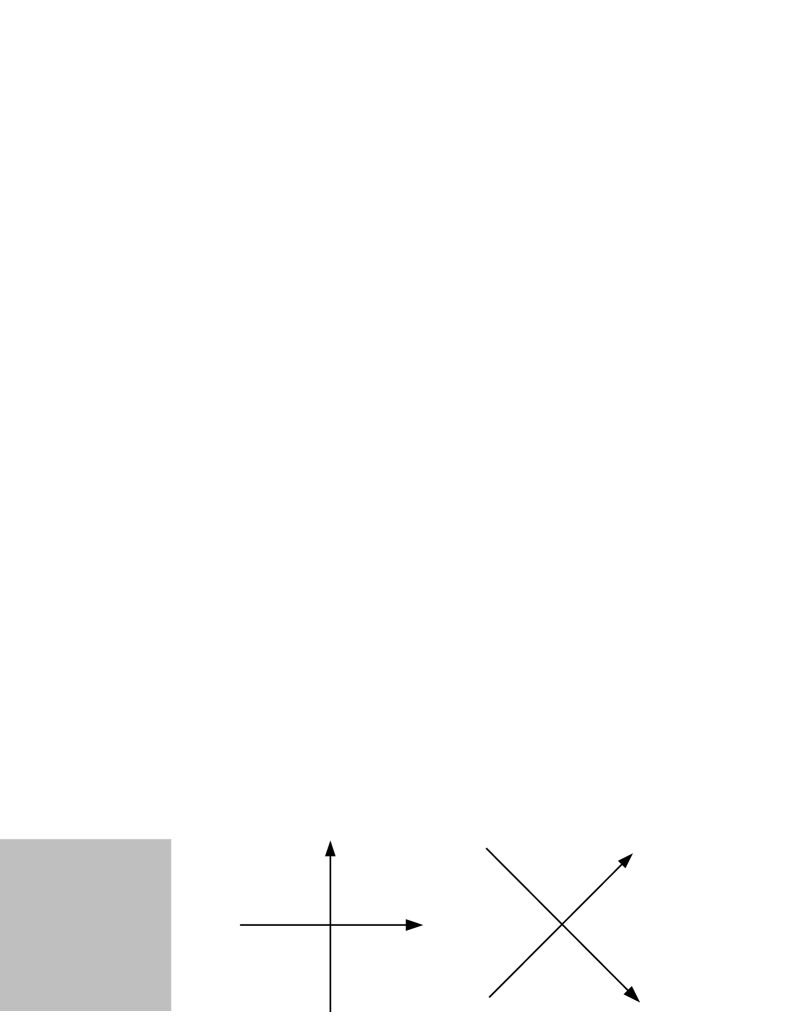
Figure 6: Breaking 2–fold degeneracy of an eigenspace to $A=\binom{0\;\;0}{0\;\;0}$ (left) in two ways $B_{N}=\binom{1\;\;0}{0\;\;1}/N$ and $C_{N}=\binom{0\;\;1}{1\;\;0}/N$ admitting no common eigenvectors (middle and right).

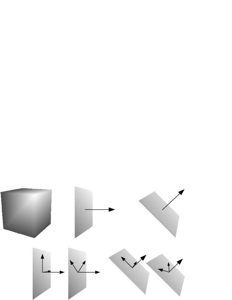
Figure 7: Construction similar to Figure 6, now iterated in 3D.

Theorem 4.3

Fix $d\in\mathbb{N}$ and consider the space $\mathbb{R}^{\binom{d}{2}}$ of real symmetric $d\times d$ matrices. Then the multivalued mapping

$$\operatorname{Diag}_{d}:\mathbb{R}^{\binom{d}{2}}\quad\ni\quad A\quad\mapsto\quad\big{\{}(\vec{w}_{1},\ldots,\vec{w}_{d})\text{ basis of $\mathbb{R}^{d}$ of eigenvectors to $A$}\big{\}}$$

has complexity $\mathfrak{C}_{\rm t}(\operatorname{Diag}_{d})=\mathfrak{C}_{\rm c}\big{(}\operatorname{Diag}_{d},\rho^{\binom{d}{2}},\rho^{d\times d}\big{)}=d$.

The lack of continuity of the mapping $\operatorname{Diag}$ is closely related to inputs with degenerate eigenvalues [ZiBr04, Example 18]. In fact our below proof yields a witness of $d$-discontinuity by constructing an iterated sequence of symmetry breakings in the sense of Mathematical Physics; cf. Figure 7. On the other hand even in the non-degenerate case, $\operatorname{Diag}$ is inherently multivalued since any permutation of a basis constitutes again a basis.

Proof (Theorem 4.3)

Let $\sigma(A)\subseteq\mathbb{R}$ denote the set (!) of eigenvalues of $A$, that is not counting multiplicities. [ZiBr04, Theorem 19] has shown that knowing $\operatorname{Card}\sigma(A)\in\{1,\ldots,d\}$ suffices to compute some orthonormal basis of eigenvectors; hence $\mathfrak{C}_{\rm t}(\operatorname{Diag})\leq\mathfrak{C}_{\rm c}\big{(}\operatorname{Diag},\rho^{\binom{d}{2}},\rho^{d\times d}\big{)}\leq d$.

For the converse inequality, we shall apply Lemma 5d); but, as in the proof of Theorem 4.1, first invoke Lemma 3b) by appending to $\operatorname{Diag}$ a computable mapping: namely orthonormalization. Indeed, standard Gram-Schmidt constitutes an effective procedure for turning a basis into an orthonormal one; and this process respects eigenspaces because those belonging to different eigenvalues are mutually orthogonal anyway. In the sequel we will therefore investigate the multivalued mapping $\operatorname{Diag}^{\prime}:\mathbb{R}^{\binom{d}{2}}\rightrightarrows\mathcal{O}(\mathbb{R},d)$ to the compact space of orthogonal matrices.
Start with symmetric $A:=0^{d\times d}$, eigenvalue $0$ being $d$–fold degenerate with eigenspace entire $\mathbb{R}^{d}$, $d\geq 2$. Now consider two unit vectors $\vec{v}$ and $\vec{w}$ neither collinear nor orthogonal. According to Remark 4.2 above there exist corresponding sequences $(B_{N})_{{}_{N}}$ and $(C_{N})_{{}_{N}}$ of symmetric matrices, both converging to $A$ and with $(d-1)$–fold degenerate eigenspaces and further 1D ones: $B_{N}\cdot\vec{v}=1/N\cdot\vec{v}$ and $C_{N}\cdot\vec{w}=1/N\cdot\vec{w}$; all eigenspaces are independent of $N$. Hence, by Observation 4.4 below, $B_{N}$ and $C_{N}$ do not admit a common eigenvector basis; i.e. $\operatorname{Diag}^{\prime}(B_{N})\cap\operatorname{Diag}^{\prime}(C_{N})=\emptyset$ for all $N$. And Lemma 6b) implies $B\big{(}\operatorname{Diag}^{\prime}(B_{N}),\epsilon\big{)}\cap B\big{(}\operatorname{Diag}^{\prime}(C_{N}),\epsilon\big{)}=\emptyset$ for some $\epsilon>0$ independent of $N$. See also Figure 6…
We have satisfied the prerequisites to Lemma 5b) and hence conclude that there is a witness of discontinuity for $\operatorname{Diag}^{\prime}$. For a witness of 2-discontinuity observe that the above construction can be iterated in case $d\geq 3$ as depicted in Figure 7: To each $B_{N}=:A^{(0)}_{N}$ there exist sequences $A^{(0,0)}_{N,M}$ and $A^{(0,1)}_{N,M}$ of symmetric matrices converging to $A^{(0)}_{N}$ uniformly in $N$ with common $(d-2)$–fold degenerate eigenspaces and further ones $A^{(0,j)}_{N,M}\cdot\vec{x}^{(0,j)}=1/M\cdot\vec{x}^{(0,j)}$ for $j=0,1$ where unit vectors $\vec{x}^{(0,0)}$ and $\vec{x}^{(0,1)}$ are neither collinear nor orthogonal; similarly sequences $A^{(1,j)}_{N,M}$ and eigenvectors $\vec{x}^{(1,j)}$ correspond to $A^{(1)}_{N}:=C_{N}$. Again, it follows $B\big{(}\operatorname{Diag}^{\prime}(A^{(i,0)}_{N,M}),\epsilon\big{)}\cap B\big{(}\operatorname{Diag}^{\prime}(A^{(i,1)}_{N,M}),\epsilon\big{)}=\emptyset$ for some $\epsilon>0$ independent of $N,M$; hence Lemma 5d) applies.
And so on, until arriving at a witness of $(d-1)$-discontinuity and at matrices $A^{(i_{1},\ldots,i_{d-1})}_{N_{1},\ldots,N_{d-1}}$ with $1$–fold (i.e. non-)degenerate eigenspaces (where we cannot apply Remark 4.2 any more). ∎

Observation 4.4

Let $B,C\in\mathbb{C}^{d\times d}$ be hermitian matrices. Let $B\cdot\vec{v}=\lambda\vec{v}$ and $C\cdot\vec{w}=\mu\vec{w}$ denote respective eigenvectors to non-degenerate eigenvalues $\lambda$ and $\mu$.
If $B$ and $C$ admit a common eigenvector basis, then $\vec{v}$ and $\vec{w}$ are either collinear or orthogonal.

4.3 Finding Some Eigenvector

Instead of computing an entire basis of eigenvectors, we now turn to the problem of determining just one arbitrary eigenvector to a given real symmetric matrix. This turns out to be considerably less ‘complex’:

Theorem 4.5

For a real symmetric $n\times n$-matrix $A$, consider the quantity

$$m(A)\quad:=\quad\min\big{\{}\dim\operatorname{kernel}(A-\lambda\operatorname{id}):\lambda\in\sigma(A)\big{\}}\quad\in\quad\{1,\ldots,n\}\enspace.$$

Given $d:=\lfloor\log_{2}m\rfloor\in\{0,1,\ldots,\lfloor\log_{2}n\rfloor\}$ and a $\rho^{\binom{n}{2}}$–name of $A$, one can $\rho^{n}$–compute (i.e. effectively find) some eigenvector of $A$.

The proof employs the following tool about certain combinatorics and computability of finite multi-sets.

Lemma 7

Let $(x_{1},\ldots,x_{n})$ denote an $n$-tuple of real numbers and consider the induced partition $\mathcal{I}:=\big{\{}\{1\leq i\leq n:x_{i}=x_{j}\}:1\leq j\leq n\big{\}}$ of the index set $\{1,\ldots,n\}=:[n]$ according to the equivalence relation $i\equiv j:\Leftrightarrow x_{i}=x_{j}$. Furthermore let $m:=\min\big{\{}\operatorname{Card}(I):I\in\mathcal{I}\big{\}}$.

1. Consider $I\subseteq[n]$ with $1\leq\operatorname{Card}(I)<2m$ such that

   $$x_{i}\neq x_{j}\quad\text{for all}\quad i\in I\quad\text{and all}\quad j\in[n]\setminus I\enspace.$$ (5)

   Then $I\in\mathcal{I}$.

2. Suppose $k\in\mathbb{N}$ is such that $k\leq m<2k$. Then there exists $I\in\mathcal{I}$ with $k\leq\operatorname{Card}(I)<2k$ satisfying (5). Conversely every $I\subseteq[n]$ with $k\leq\operatorname{Card}(I)<2k$ satisfying (5) has $I\in\mathcal{I}$.

3. Given a $\rho^{n}$–name of $(x_{1},\ldots,x_{n})$ and given $k\in\mathbb{N}$ with $k\leq m<2k$, one can computably find some $I\in\mathcal{I}$.

4. Given a $\rho^{n}$–name of $(x_{1},\ldots,x_{n})$ and given $\operatorname{Card}(\mathcal{I})$, one can compute $\mathcal{I}$.

Claim c) can be considered a weakening of Claim d) which had been established in [ZiBr04, Proposition 20].

Proof

1. Take $i\in I$, $i\in J$ for some $J\in\mathcal{I}$. Then obviously $I\supseteq J$, because $j\in J\setminus I$ would imply $x_{i}=x_{j}$: contradicting Equation (5).
   It remains to show $I\subseteq J$. Suppose that $x_{i}\neq x_{i^{\prime}}$ for some $i^{\prime}\in I$. Then $i^{\prime}\in J^{\prime}$ for some $J^{\prime}\in\mathcal{I}$ disjoint to $J$. Thus condition “$x_{i}\neq x_{j}$” fails for all $j\in J$; and “$x_{i^{\prime}}\neq x_{j}$” fails for all $j\in J^{\prime}$: i.e. for a total of $\operatorname{Card}(J)+\operatorname{Card}(J^{\prime})\geq 2m$ choices of $j\in[n]$, whereas by Equation (5) it is supposed to hold for all $j\in[n]\setminus I$: a total of $>n-2m$ choices—contradiction.

2. For the first claim, simply choose $I\in\mathcal{I}$ with $\operatorname{Card}(I)=m$. Concerning the second claim, observe that $k\leq m$ and $\operatorname{Card}(I)<2k$ imply $\operatorname{Card}(I)<2m$; hence Item a) applies.

3. Recall that inequality of real numbers is ‘semi-decidable’; formally: $\{(x,y):x\neq y\}\subseteq\mathbb{R}^{2}$ is $\rho^{2}$–r.e. open in $\mathbb{R}^{2}$ in the sense of [Weih00, Definition 3.1.3.2]. Hence we may simultaneously try every $I\subseteq[n]$ with $k\leq\operatorname{Card}(I)<2k$ and semi-decide Condition (5): according to Item b) this will succeed precisely for some $I\in\mathcal{I}$. ∎

Proof (Theorem 4.5)

Compute according to [ZiBr04, Proposition 17] some ($\rho^{n}$–name of an) $n$-tuple of eigenvalues $(\lambda_{1},\ldots,\lambda_{n})$ of $A$, repeated according to their multiplicities. Now due to [ZiBr04, Theorem 11], (some eigenvector in) the eigenspace $\operatorname{kernel}(A-\lambda_{i}\operatorname{id})$ can be computably found when knowing $\operatorname{rank}(A-\lambda_{i}\operatorname{id})$ (recall Theorem 4.1), that is the multiplicity of $\lambda_{i}$ in the multi-set $(\lambda_{1},\ldots,\lambda_{n})$. To this end we apply Lemma 7c), observing $k:=2^{d}\leq m<2k$ since $d=\lfloor\log_{2}m\rfloor$. ∎

Theorem 4.6

The multivalued mapping

$$\operatorname{EVec}_{n}:\mathbb{R}^{\binom{n}{2}}\quad\ni\quad A\quad\mapsto\quad\{\vec{w}\text{ eigenvector of }A\}$$

has complexity $\mathfrak{C}_{\rm t}(\operatorname{EVec}_{n})=\mathfrak{C}_{\rm c}\big{(}\operatorname{EVec}_{n},\rho^{\binom{n}{2}},\rho^{n}\big{)}=\lfloor\log_{2}n\rfloor+1$.

Remark 4.7

1. In $\mathbb{K}^{2m}$, the two subspaces $U:=\{(x_{1},\ldots,x_{m},0,\ldots,0):x_{i}\in\mathbb{K}\}$ and $V:=\{(x_{1},\ldots,x_{m},x_{1},\ldots,x_{m}):x_{i}\in\mathbb{K}\}$, as well as their orthogonal complements $U^{\bot}=\{(0,\ldots,0,x_{1},\ldots,x_{m}):x_{i}\in\mathbb{K}\}$ and $V^{\bot}=\{(x_{1},\ldots,x_{m},-x_{1},\ldots,-x_{m}):x_{i}\in\mathbb{K}\}$, have dimension $m$ and satisfy $\{0\}=U\cap V=U\cap V^{\bot}=U^{\bot}\cap V=U^{\bot}\cap V^{\bot}$.

2. Write $W^{(0)}_{0}:=U$, $W^{(0)}_{1}:=U^{\bot}$, $W^{(1)}_{0}:=V$, and $W^{(1)}_{1}:=V^{\bot}$. Applying the above construction to each of them again, we iteratively obtain in $\mathbb{K}^{2^{d}}$ subspaces $W^{(j_{1},\ldots,j_{k})}_{i_{1},\ldots,i_{k}}$ of dimension $2^{d-k}$ ($0\leq k\leq d$, $i_{\ell},j_{\ell}=0,1$) with the following properties:

   1. $\displaystyle W^{(\bar{\jmath})}_{\bar{\imath}}\bot W^{(\bar{\jmath})}_{\bar{\imath}^{\prime}}$ for all $\bar{\imath},\bar{\imath}^{\prime},\bar{\jmath}\in\{0,1\}^{k}$, $\bar{\imath}\neq\bar{\imath}^{\prime}$.

   2. $\displaystyle W^{(j_{1},\ldots,j_{k+1})}_{i_{1},\ldots,i_{k+1}}\subseteq W^{(j_{1},\ldots,j_{k})}_{i_{1},\ldots,i_{k}}$

   3. For any choice of $\displaystyle U_{\bar{\imath}}\in\big{\{}W^{(\bar{\jmath})}_{\bar{\imath}}:\bar{\jmath}\big{\}}$, it holds $\bigcap_{\bar{\imath}}U_{\bar{\imath}}=\{0\}$.

3. Let $A:\mathbb{C}^{n}\to\mathbb{C}^{n}$ denote an hermitian linear map with $2m$–fold degenerate eigenvalue $\lambda\in\mathbb{R}$. Let $W^{(j)}_{i}$ denote $m$-dimensional subspaces of $\operatorname{kernel}(A-\lambda\operatorname{id})$ according to Item a), i.e. such that $W^{(j)}_{0}\bot W^{(j)}_{1}$ and $W^{(0)}_{0}\cap W^{(1)}_{1}=\{0\}=W^{(0)}_{1}\cap W^{(1)}_{0}$. Then to every sufficiently small $\epsilon>0$ and $j=0,1$ there is a hermitian linear map $A^{(j)}:\mathbb{C}^{n}\to\mathbb{C}^{n}$ with

   • $\displaystyle A^{(j)}\big{|}_{\operatorname{kernel}(A-\lambda\operatorname{id})^{\bot}}\;\equiv\;A\big{|}_{\operatorname{kernel}(A-\lambda\operatorname{id})^{\bot}}$

   • $\|A-A^{(j)}\|\leq\epsilon$;

   • $A^{(j)}$ is real if $A$ was.

   • $\displaystyle A^{(j)}\big{|}_{\operatorname{kernel}(A-\lambda\operatorname{id})}$ has eigenspaces $W^{(j)}_{0}$ and $W^{(j)}_{1}$

   • to different eigenvalues distinct from those of $A$

   In particular, eigenvectors of $A^{(j)}$ lie in $\operatorname{kernel}(A-\lambda\operatorname{id})^{\bot}\cup W^{(j)}_{0}\cup W^{(j)}_{1}$.

Proof (Theorem 4.6)

Theorem 4.5 shows that $\operatorname{EVec}_{n}$ is $(d+1)$-computable for $d:=\lfloor\log_{2}n\rfloor$. It remains to show the existence of a witness of $d$-discontinuity, and w.l.o.g. $n=2^{d}$. To this end, start with $A:=0$ and $A^{(j)}_{N}$ ($j=0,1$) according to Remark 4.7c) with $\epsilon:=1/N$, $\lambda:=0$, $m:=2^{d-1}$. It follows $\operatorname{EVec}(A^{(j)})\subseteq W^{(j)}_{0}\cup W^{(j)}_{1}$, thus $\operatorname{EVec}(A^{(0)})\cap\operatorname{EVec}(A^{(1)})=\emptyset$; hence $B\big{(}\tilde{\operatorname{EVec}}(A^{(0)}),\delta\big{)}\cap B\big{(}\tilde{\operatorname{EVec}}(A^{(1)}),\delta\big{)}=\emptyset$ for some $\delta>0$ according to Lemma 6b) where $\tilde{\operatorname{EVec}}:=\operatorname{norm}\circ\operatorname{EVec}:\mathbb{R}^{\binom{n}{2}}\to\mathcal{S}^{n-1}$ has compact range and, by virtue of Lemma 3b), the same complexity of non-uniform computability as $\operatorname{EVec}$. This yields, according to Lemma 5b), (in a complicated way) a witness of discontinuity of $\operatorname{EVec}$.
Now iterating Remark 4.7c) with the subspaces according to Remark 4.7b), we obtain matrix sequences $A^{(j_{1},\ldots,j_{k})}_{n_{1},\ldots,n_{k}}$ for $1\leq k\leq d$ and $j_{1},\ldots,j_{k}\in\{0,1\}$ and $n_{1},\ldots,n_{k}\in\mathbb{N}$ with $\displaystyle\operatorname{EVec}(A^{(\bar{\jmath})}_{\bar{n}})\subseteq\bigcup\nolimits_{\bar{\imath}\in\{0,1\}^{k}}W^{(\bar{\jmath})}_{\bar{\imath}}$ for each $\bar{\jmath}\in\{0,1\}^{k}$; hence

$$\bigcap\nolimits_{\bar{\jmath}\in\{0,1\}^{k}}\operatorname{EVec}(A^{(\bar{\jmath})}_{\bar{n}})\quad\subseteq\quad\bigcap\nolimits_{\bar{\jmath}}\bigcup\nolimits_{\bar{\imath}}W^{(\bar{\jmath})}_{\bar{\imath}}\quad=\quad\{0\}$$

by Remark 4.7b(i-iii). Therefore $\bigcap\nolimits_{\bar{\jmath}\in\{0,1\}^{k}}B\big{(}\tilde{\operatorname{EVec}}(A^{(\bar{\jmath})},\epsilon\big{)}=\emptyset$ for some $\epsilon>0$ according to Lemma 6b). So Lemma 5d) finally yields a witness of $d$-discontinuity. ∎

4.4 Root Finding

We now address the effective Intermediate Value Theorem [Weih00, Theorem 6.3.8.1]. Closely related is the problem of selecting from a given closed non-empty interval some point, recall Example 1.3d). Both are treated quantitatively within our complexity-theoretic framework.

Specifically concerning Example 1.3d), observe that any non-degenerate interval $[a,b]$ contains a rational (and thus computable) point $x$; and providing an integer numerator and denominator of $x$ makes the problem of computably selecting some $x$ from given $[a,b]$ trivial. On the other hand, rational numbers may require arbitrarily large descriptions; even more, there are intervals containing rationals only of such large Kolmogorov Complexity; cf. Claim d) of the following

Remark 4.8

1. There exists an unbounded function $\varphi:\mathbb{N}\to\mathbb{N}$ such that the Kolmogorov Complexity $C(m)$ of any integer $m\geq n$ is at least $\varphi(n)$.

2. Fix $q\in\{2,3,\ldots\}$. For $x\in[0,1)\cap\mathbb{Q}$, $x=r/s=\sum_{i=1}^{\infty}a_{i}q^{-i}$, $r,s\in\mathbb{Z}$ coprime and $a_{i}\in\{0,1,\ldots,q-1\}$, $C(r,s)$ and $C\big{(}(a_{i})_{{}_{i}}\big{)}$ agree up to some constant independent of $x$ (but possibly depending on $q$).

That is, just like the usual Kolmogorov Complexity (of a binary string or integer) depending up to an additive constant on the universal machine under consideration [LiVi97, Theorem 2.1.1], the complexity $C(x)$ of a rational number $x\in\mathbb{Q}$ is well-defined up to $\pm\mathcal{O}(1)$.

1. For $a,b\in\mathbb{Q}$, $C(a+b),C(a-b),C(a\cdot b),C(a/b)\leq C(a)+C(b)+\mathcal{O}(1)$.
   To every $a\in\mathbb{Q}$ there exists $\bar{\sigma}\in\Sigma^{\omega}$ with $C(a)\leq C(\bar{\sigma})+\mathcal{O}(1)$, the latter in the sense of Proposition 2.

2. Let $x\in\mathbb{R}$ be algebraic of degree 2 (e.g. $x=\sqrt{p}+q$ for some prime number $p\in\mathbb{P}$ and $q\in\mathbb{Q}$). Then there exists $\varepsilon>0$ such that for all $r,s\in\mathbb{Z}$ with $s>0$, $|x-r/s|>\varepsilon/s^{2}$.

3. Given $N\in\mathbb{N}$, there exist $a,b\in\mathbb{Q}\cap[0,1]$ such that all $x\in\mathbb{Q}\cap[a,b]$ have $C(x)\geq N$.

Proof

1. is from [LiVi97, Theorem 2.3.1i].

2. On the one hand, a constant-size program can easily convert $(r,s)$ to the sequence $(a_{i})$; hence $C\big{(}(a_{i})_{{}_{i}}\big{)}\leq C(r,s)+c$. Concerning a converse inequality, $x=\sum_{i=1}^{\infty}a_{i}q^{-i}\in\mathbb{Q}$ implies that $(a_{i})_{{}_{i}}$ be periodic after some initial segment; i.e. $a_{i}=a_{i+n}=a_{i+2n}=\ldots$ for all $i\geq m$; hence

   $$x = \underbrace{\sum\nolimits_{i<m}a_{i}q^{-i}}_{=:u}+\Big{(}\underbrace{\sum\nolimits_{i=0}^{n-1}a_{m+i}q^{n-i}}_{=:v}\Big{)}\cdot\big{(}q^{-m-n}+q^{-m-2n}+q^{-m-3n}+\cdots\big{)}\quad=$$

   $$= u+v\cdot q^{-m}/(q^{n}-1)$$

   with $u\in\mathbb{Q}$ and $v,q^{-m}/(q^{n}-1)\in\mathbb{Z}$ which can easily be converted into coprime $r,s$ with $x=r/s$. Also both $m$ (the length of the initial segment) and $n$ (the period) need not be stored separately but can be sought for computationally within the sequence $(a_{i})$.

3. It is easy, and uses only constant size overhead, to combines Turing machines computing $a$ and $b$ into ones computing $a+b$, $a-b$, $a\times b$, and $a/b$, respectively. Moreover a machine computing numerator and denominator of $a$ can be adapted to calculate a $\rho$–name $\bar{\sigma}$ of $a$.

4. is Liouville’s Theorem on Diophantine approximation.

5. Take $x\in(1/3,2/3)$ algebraic of degree 2, $\varepsilon>0$ according to c). Choose $0<\delta<1/3$ such that $\varphi(\sqrt{\varepsilon/\delta})>N$. Then $\mathbb{Q}\ni r/s\in[x-\delta,x+\delta]$ requires $\varepsilon/s^{2}<\delta$, hence $s>\sqrt{\varepsilon/\delta}$ and $C(x)=C(r,s)\geq C(s)\geq N$. ∎

Note that Remark 4.8e) applies only to rational numbers; that is $[a,b]$ might still contain, say, algebraic reals $x$ of low Kolmogorov complexity. We now extend the claim to computable elements: Referring to Proposition 2, Theorem 4.9b) below shows that, even with the help of negative information about (i.e. a $\psi_{\!\raisebox{0.60275pt}{${\scriptscriptstyle>}$}}$–name of) a given interval $[a,b]$, unbounded discrete advice is in general necessary to find (a $\rho$–name of) some $x\in[a,b]$.

Theorem 4.9

1. Finding a zero of a given continuous function $f:[0,1]\to[-1,+1]$ with $f(0)=-1$ and $f(1)=+1$, that is the multivalued mapping $\operatorname{Intermed}:\subseteq C[0,1]\rightrightarrows[0,1]$,

   $$f\mapsto f^{-1}[0]\text{ on }\operatorname{dom}(\operatorname{Intermed}):=\big{\{}f:[0,1]\to[-1,+1]\text{ continuous},f(1)=1=-f(0)\big{\}}\enspace,$$

   has $\mathfrak{C}_{\rm c}(\operatorname{Intermed},[\rho\!\to\!\rho],\rho)=\mathfrak{C}_{\rm t}(\operatorname{Intermed})=\omega$.

2. Selecting some point from a given co-r.e. closed bounded non-degenerate interval, specifically the multivalued mapping

   $$\operatorname{Select}:[a,b]\mapsto[a,b],\qquad\operatorname{dom}(\operatorname{Select}):=\{[a,b]:0\leq a<b\leq 1\}\enspace,$$

   is not $d$-wise $(\psi_{\!\raisebox{0.60275pt}{${\scriptscriptstyle>}$}},\rho)$–continuous for any $d\in\mathbb{N}$.

Discontinuity of $\operatorname{Intermed}$ is well-known due to, and to occur for, arguments $f$ which ‘hover’ [Weih00, Theorem 6.3.2]. We iterate this property to obtain a witness of $d$-discontinuity for arbitrary $d\in\mathbb{N}$:

Figure 8: Witness of discontinuity for the effective Intermediate Value Theorem.

Remark 4.10

1. Consider the piecewise linear, continuous function $f:[0,1]\to[-1,+1]$,

   $$f(x):=3x-1\text{ for }x\in[0,1/3],\quad f:\equiv 0\text{ on }[1/3,2/3],\quad f(x):=3x-2\text{ for }x\in[2/3,1]\enspace.$$

   Then $A:=[1/3,5/12]$ and $B:=[7/12,2/3]$ lie in $f^{-1}[0]=[1/3,2/3]=:I$. Moreover to $n>0$ there are piecewise linear continuous functions $g,h\in\operatorname{dom}(\operatorname{Intermed})$ with $g^{-1}[0]=A$ and $h^{-1}[0]=B$ and $\|f-g\|_{\infty},\|f-h\|_{\infty}<1/n$; cf. Figure 8.
   In particular, $B\big{(}\operatorname{Intermed}(g),1/27\big{)}\cap B\big{(}\operatorname{Intermed}(h),1/27\big{)}=\emptyset$.

2. Let $f^{()}:=f$, $I^{()}:=I$, $f^{(0)}_{n}:=g$, $I^{(0)}:=A$, $f^{(1)}_{n}:=h$, $I^{(1)}:=B$.
   Iterating the above construction we obtain, to every $d\in\mathbb{N}$ and $(i_{1},\ldots,i_{d})\in\{0,1\}^{d}$, closed intervals $I^{(i_{1},\ldots,i_{d})}$

   1. of length $3^{-d-1}$

   2. with $I^{(i_{1},\ldots,i_{d-1},i_{d})}\subseteq I^{(i_{1},\ldots,i_{d-1})}$

   3. such that $B\big{(}I^{(i_{1},\ldots,i_{d-1},0)},3^{-d-2}\big{)}\cap B\big{(}I^{(i_{1},\ldots,i_{d-1},1)},3^{-d-2}\big{)}=\emptyset$.

   and sequences of functions $f^{(i_{1},\ldots,i_{d})}_{n_{1},\ldots,n_{d}}\in\operatorname{dom}(\operatorname{Intermed})$ with

   1. $f^{(i_{1},\ldots,i_{k})}_{n_{1},\ldots,n_{k}}=\operatorname*{ulim}_{m}f^{(i_{1},\ldots,i_{k},\ldots,i_{d})}_{n_{1},\ldots,n_{k},m,\ldots,m}$

   2. and $\big{(}f^{(i_{1},\ldots,i_{d})}_{n_{1},\ldots,n_{d}}\big{)}^{-1}[0]=I^{(i_{1},\ldots,i_{d})}$

   where $\phi=\operatorname*{ulim}_{m}\phi_{m}$ means $\lim_{m\to\infty}\|\phi-\phi_{n}\|_{\infty}\to 0$.

3. Let $A\subseteq B\subseteq\mathbb{R}^{d}$ and $f:\mathbb{R}^{d}\to\mathbb{R}$ continuous with $f(\vec{x})\leq d_{B}(\vec{x})$ for all $\vec{x}\in\mathbb{R}^{d}$. Then there exists a sequence of continuous functions $g_{\ell}:\mathbb{R}^{d}\to\mathbb{R}$ with $g_{1}=f$ and $d_{A}(\vec{x})=\sup_{\ell}g_{\ell}(\vec{x})$:
   namely $g_{\ell}:=f\cdot 1/\ell+(1-1/\ell)\cdot d_{A}$.

Proof (Theorem 4.9)

1. As has been frequently exploited before [Weih00, Section 6.3], $f\in\operatorname{dom}(\operatorname{Intermed})$ has an entire interval of zeros or has some isolated root. In the latter case, such a root can be found according to [Weih00, Theorem 6.3.7]. In the former case, that interval contains a rational one—which can be provided explicitly by its numerator and denominator as (unbounded) discrete advice. We thus have shown $\mathfrak{C}_{\rm c}(\operatorname{Intermed})\leq\omega$.
   Conversely, Remark 4.10b) implies in connection with Lemma 5d) that $\operatorname{Intermed}$ is not $d$-continuous for any $d\in\mathbb{N}$.

2. Consider the intervals $I^{(i_{1},\ldots,i_{d})}$ from Remark 4.10b). However Lemma 5d) does not apply directly since the space of closed (non-degenerate) sub-intervals of $[0,1]$ is, equipped with representation $\psi_{\!\raisebox{0.60275pt}{${\scriptscriptstyle>}$}}$ rather than with $\psi$ [Weih00, Theorem 5.2.9], not metric. Instead, we resort to Lemma 4 as follows: Suppose $F$ is a $(\psi_{\!\raisebox{0.60275pt}{${\scriptscriptstyle>}$}},\rho)$–realizer of $\operatorname{Select}$ and recall that a $\psi_{\!\raisebox{0.60275pt}{${\scriptscriptstyle>}$}}$–name of closed $\emptyset\not=B\subseteq[0,1]$ is a sequence of continuous functions $g_{\ell}:[0,1]\to\mathbb{R}$ with $d_{B}(x)=\sup_{\ell}g_{\ell}(x)$. By Remark 4.10c), any (initial segment of) such a name can be slightly perturbed to one of $A\subseteq B$.
   So start with such a sequence $g^{()}=(g_{\ell})_{{}_{\ell}}$ for $I^{()}$; then take a sequence of sequences $g^{(0)}_{n,\ell}$ with $g^{(0)}_{n,\ell}:=g_{\ell}$ for $\ell\leq n$ and $\sup_{\ell}g^{(0)}_{n,\ell}(x)=d_{I^{(0)}}(x)$ according to Remark 4.10c); that is, $(g^{(0)}_{n,\ell})_{{}_{\ell}}$ is a $\psi_{\!\raisebox{0.60275pt}{${\scriptscriptstyle>}$}}$–name of $I^{(0)}\subseteq I^{()}$ ‘resembling’ a $\psi_{\!\raisebox{0.60275pt}{${\scriptscriptstyle>}$}}$–name $I^{()}$ for $\ell\leq n$. In particular, $g^{()}_{\ell}=\operatorname*{ulim}_{n}g^{(0)}_{n,\ell}$ uniformly in $x$ and $\ell$. Similarly take $g^{(1)}_{n,\ell}$ corresponding to $I^{(1)}$ initially resembling $I^{()}$. Because of Remark 4.10b iii), Lemma 5b) yields a witness of discontinuity for $F$.
   Now iterate this construction with the intervals $I^{(n_{1},\ldots,n_{d})}$ from Remark 4.10b) to obtain a witness of $d$-discontinuity according to Lemma 5c). ∎

5 Conclusion, Extensions, and Perspectives

We claim that a major source of criticism against Recursive Analysis misses the point: although computable functions $f$ are necessarily continuous when given approximations to the argument $x$ only, most practical $f$’s do become computable when providing in addition some discrete information about $x$. Such ‘advice’ usually consists of some very natural and mathematically explicit integer value from a bounded range (e.g. the rank of the matrix under consideration) and is readily available in practical applications.

We have then turned this observation into a complexity theory, investigating the minimum size (=cardinal) of the range this discrete information comes from. And we have determined this quantity for several simple and natural problems from linear algebra: calculating the rank of a given matrix, solving a system of linear equalities, diagonalizing a symmetric matrix, and finding some eigenvector to a given symmetric matrix. The latter three are inherently multivalued. And they exhibit a considerable difference in complexity: for input matrices of format $n\times n$, usually discrete advice of order $\Theta(n)$ is necessary and sufficient; whereas some single eigenvector can be found using only $\Theta(\log n)$–fold advice: specifically, the quantity $\big{\lfloor}\log_{2}\min\big{\{}\dim\operatorname{kernel}(A-\lambda\operatorname{id}):\lambda\in\sigma(A)\big{\}}\big{\rfloor}$. The algorithm exploits this data based on some combinatorial considerations—which nicely complement the heavily analytical and topological arguments usually dominant in proofs in Recursive Analysis.

Our lower bound proofs assert $d$-discontinuity of the function under consideration. They can be extended (yet become even more tedious when trying to do so formally) to weak $d$-discontinuity. Also the major tool for such proofs, namely that of witnesses of $d$-discontinuity, would deserve generalizing from effective metric to computable topological spaces.

5.1 Non-Integral Advice

Theorem 4.1 shows that $d$-fold advice does not suffice for effectively finding a nontrivial solution $\vec{x}$ to a homogeneous equation $A\cdot\vec{x}=0$; whereas $(d+1)$-fold advice, namely providing $\operatorname{rank}(A)\in\{0,\ldots,d\}$, does suffice.

• Since the rank can be effectively approximated from below (i.e. is $\rho_{\raisebox{0.60275pt}{${\scriptscriptstyle<}$}}$-computable) [ZiBr04, Theorem 7], it in fact suffices to provide complementing upper approximations (i.e. a $\rho_{\raisebox{0.60275pt}{${\scriptscriptstyle>}$}}$–name) to $\operatorname{rank}(A)$. One may say that this constitutes strictly less than $(d+1)$-fold information.

• Similarly concerning diagonalization of a real symmetric $n\times n$-matrix $A$, since the number $\operatorname{Card}\sigma(A)$ of distinct eigenvalues can be effectively approximated from below, it suffices to provide only complementing upper approximations—cmp. [ZiBr04, Theorem 19]—which may be regarded as strictly less than $n$-fold advice.

• Similarly, with respect to the problem of finding some eigenvector of $A$, again strictly less than $(\lfloor\log_{2}n\rfloor+1)$-fold advice suffices: namely lower approximations to $\lfloor\log_{2}m(A)\rfloor$ (with $m(A)$ from Theorem 4.5) based on the following

Observation 5.1

The mapping $\mathbb{R}^{\binom{n}{2}}\ni A\mapsto\lfloor\log_{2}m(A)\rfloor$ is $(\rho^{n\cdot(n-1)/2},\rho_{\raisebox{0.60275pt}{${\scriptscriptstyle>}$}})$–computable.

Proof

Given $\lambda$, $\dim\operatorname{kernel}(A-\lambda\operatorname{id})=n-\operatorname{rank}(A-\lambda\operatorname{id})$ is $\rho_{\raisebox{0.60275pt}{${\scriptscriptstyle>}$}}$–computable by [ZiBr04, Theorem 7i]; hence so is its minimum $m(A)$ over all $\lambda\in\sigma(A)$, cmp. [ZiBr04, Proposition 17] and [Weih00, Exercise 4.2.11]. Now although $\log_{2}:(0,\infty)\ni x\mapsto\ln(x)/\ln(2)\in\mathbb{R}$ is $(\rho_{\raisebox{0.60275pt}{${\scriptscriptstyle>}$}},\rho_{\raisebox{0.60275pt}{${\scriptscriptstyle>}$}})$–computable by monotonicity, $x\mapsto\lfloor x\rfloor$ is of course not. On the other hand, $m(A)$ attains only integer values; and the nondecreasing, purely integral function $\mathbb{N}\ni m\mapsto\lfloor\log_{2}m\rfloor\in\mathbb{N}_{0}$ is $(\rho_{\raisebox{0.60275pt}{${\scriptscriptstyle>}$}},\rho_{\raisebox{0.60275pt}{${\scriptscriptstyle>}$}})$–computable. ∎

The above examples suggest refining $k$-fold advice to non-integral values of $k$:

Definition 7

Let $f:X\to Y$ be a function and $Z$ a topological $\text{T}_{0}$ space.

1. Call $f$ continuous with $Z$-advice if there exists a function $g:X\to Z$ such that the function $f|^{g}$, defined as follows, is continuous:

   $$\operatorname{dom}(f|^{g})\;:=\;\{(x,z):x\in X,g(x)=z\}\;\subseteq\;X\times Z,\qquad(x,z)\mapsto f(x)\enspace.$$ (6)

2. Let $Z$ be finite and fix some injective notation $\nu_{Z}:\subseteq\Sigma^{*}\to\tau$ of the (finitely many) open subsets of $Z$. Then the representation $\delta_{Z}=\delta_{Z,\nu_{Z}}:\subseteq\Sigma^{\omega}\to Z$ is defined as follows:
   $\bar{\sigma}\in\Sigma^{\omega}$ is a $\delta_{Z,\nu}$-name of $z$  iff  it is a $\nu$-enumeration (with arbitrary repetition) of all open sets containing $Z$.

3. For effective metric spaces $(X,\alpha)$ and $(Y,\beta)$, call $f$ $(\alpha,\beta)$-computable with $Z$-advice if there exists some $g:X\to Z$ such that the function $f|^{g}:\subseteq X\times Z\to Y$ from a) is $(\alpha\times\delta_{Z},\beta)$-computable.

Restricting $Z$ to discrete spaces, one recovers Definition 1a):

Lemma 8

For $d\in\mathbb{N}$ let $Z_{d}$ denote the set $\{0,1,\ldots,d-1\}$ equipped with the discrete topology.

1. A function $f:X\to Y$ is $d$-continuous  iff  it is continuous with $Z_{d}$-advice.

2. The representation $\delta_{Z_{d}}$ of $Z_{d}$ is computably equivalent to $\nu_{Z_{d}}$: $\delta_{Z_{d}}\equiv\nu_{Z_{d}}$. Whereas in general, $\nu_{Z}$ is only computably reducible to (but not from) $\delta_{Z}$: $\nu_{Z}\precneq\delta_{Z}$.

3. A function $f:X\to Y$ is $(\alpha,\beta)$-computable with $d$-wise advice  iff  it is $(\alpha,\beta)$-computable with $Z_{d}$ advice.

4. $(Z,\delta_{Z})$ is admissible. In particular if $(X,\alpha)$ and $(Y,\beta)$ are admissible and it function $f:X\to Y$ is $(\alpha,\beta)$-computable with $Z$-advice, then $f$ is continuous with $Z$-advice.

Proof

1. Let $\Delta=\{D_{0},D_{1},\ldots,D_{d-1}\}$ denote an $d$-element partition of $X$ such that $f|_{D_{z}}$ is continuous for each $z=0,1,\ldots,d-1$. Define $g:X\ni x\mapsto$the unique $z\in Z_{d}$ with $x\in D_{z}$. Then, for open $V\subseteq Y$,

   $$(f|^{g})^{-1}[V]\quad=\quad\biguplus_{z\in Z}\big{(}f^{-1}[V]\cap\underbrace{g^{-1}[\{z\}]}_{=D_{z}}\big{)}\times\{z\}\quad=\quad\biguplus_{z\in Z}\underbrace{(f|_{D_{z}})^{-1}[V]}_{\text{open in }D_{z}}\times\{z\}$$ (7)

   is relatively open in $\biguplus_{z\in Z}D_{z}\times\{z\}=\operatorname{dom}(f|^{g})$, i.e. $f|^{g}$ continuous.
   Conversely let $f|^{g}$ be continuous for $g:X\to Z_{d}$. Define $\Delta:=\{D_{0},D_{1},\ldots,D_{d-1}\}$ where $D_{z}:=g^{-1}[\{z\}]$ for $z\in Z_{d}$. Then Equation (7) requires that $\bigcup_{z}\big{(}f^{-1}[V]\cap D_{z}\big{)}\times\{z\}$ be open in $\bigcup_{z}D_{z}\times\{z\}$. Now $D_{z}\times\{z\}$ is open by definition of the product topology and because $z\in Z_{d}$ is discrete, this implies that also the intersection $(f|^{g})^{-1}[V]\cap(D_{z}\times\{z\})=(f^{-1}[V]\cap D_{z})\times\{z\}$ be open in $D_{z}\times\{z\}$, i.e. that $f|_{D_{z}}^{-1}[V]$ is open in $D_{z}$; hence $f|_{D_{z}}$ is continuous for each $z\in Z_{k}$.

2. Since $Z$ is finite and $\nu_{Z}:\subseteq\Sigma^{*}\to Z$ is injective, everything is bounded a priori. For instance, given a $\nu_{Z}$-name of $z\in Z$, one can easily produce a pre-stored list of all (finitely many) open sets containing this $z$: thus showing $\nu_{Z}\preceq\delta_{Z}$.
   For the converse, exploit that $Z_{d}$ bears the discrete topology and therefore is effectively $\text{T}_{1}$[Weih09]: Given an enumeration of all (finite) open sets $U_{i}$ containing $z\in Z_{d}$, their intersection $\bigcap_{i}U_{i}$ becomes a singleton after finite time, thereby identifying $z$.
   In the Sierpiński space $\mathbb{S}$ from Example 5.2a) below, (some $\delta_{\mathbb{S}}$-names of) $1=\bot$ cannot continuously be distinguished from (a $\delta_{\mathbb{S}}$-name of) $0=\top$.

3. Suppose that $f|_{D_{z}}$ be $(\alpha,\beta)$-computable for each $z\in Z_{d}$. Since $Z_{d}$ is finite, it follows that $f|^{g}:(x,z)\mapsto f|_{D_{z}}(x)$ is $(\alpha\times\nu_{Z_{d}},\beta)$-computable and hence $(\alpha\times\delta_{Z_{d}},\beta)$-computable by b).
   Conversely let $f|^{g}$ be $(\alpha\times\delta_{Z_{d}},\beta)$-computable. Then, similarly to a) and since each $z\in Z_{d}$ is $\delta_{Z_{d}}$-computable, it follows that also the all restrictions $f|_{D_{z}}$ be $(\alpha,\beta)$-computable for $z\in Z_{d}$ where $D_{z}=g^{-1}[\{z\}]$.

4. Observe that $\delta_{Z}$ coincides with the standard representation of the (finite, hence effective) $\text{T}_{0}$-space $Z$; compare [Weih00, Section 3.2]. Concerning the second claim, [Weih00, Corollary 3.2.12] reveals that $f|^{g}$ is continuous. ∎

In this sense, Example 1.1 turns out to suffice with even strictly less than 2-fold advice:

Example 5.2

1. Consider as $Z$ the Sierpiński space $\mathbb{S}$, i.e. the set $\{0,1\}$ equipped with the topology $\big{\{}\emptyset,\{0\},\{0,1\}\big{\}}$ as open sets. Then the characteristic function of the complement of the Halting problem $\mathbf{1}_{\mathbb{N}\setminus H}:\mathbb{N}\to\mathbb{S}$ is $(\nu,\delta_{\mathbb{S}}$)-computable, but $\mathbf{1}_{H}$ itself is not.

2. The Gauß Staircase function $f:=\lfloor\,\cdot\,\rfloor:\mathbb{R}\to\mathbb{Z}$ is $(\rho,\rho)$-computable with $\mathbb{S}$-advice.

3. Generalizing $\mathbb{S}=:\mathbb{S}_{1}$, denote by $\mathbb{S}_{d}$ the set $\{0,1,\ldots,d\}$ equipped with the following topology: $\big{\{}\emptyset,\{0\},\{0,1\},\{0,1,2\},\ldots,\{0,1,2,\ldots,d\}\big{\}}$. Then $\operatorname{rank}:\mathbb{R}^{d\times d}\to\{0,1,\ldots,d\}$ is $(\rho^{d\times d},\rho)$-computable with $\mathbb{S}_{d}$-advice.

4. For each function $f$ and integer $d$, continuity/computability with $\mathbb{S}_{d-1}$-advice implies continuity/computability with $\mathbb{S}_{d}$-advice, implies continuity/computability with $Z_{d+1}$-advice, implies continuity/computability with $Z_{d+2}$-advice.
   On the other hand, the Dirichlet Function $\mathbf{1}_{\mathbb{Q}}:[0,1]\subseteq\mathbb{R}\to\{0,1\}$ is computable with $Z_{2}$-advice but not continuous with $\mathbb{S}_{d}$-advice for any $d\in\mathbb{N}$.

In view of [ZiBr04, Theorem 11], Example 5.2c) shows that $\mathbb{S}_{d}$-advice renders also $\operatorname{LinEq}_{n,m}$ computable for $d:=\min(n,m-1)$.

Proof (Example 5.2)

1. Simulate the given Turing machine $M$, and for each step append “$\{0,1\}$” to the $\delta_{\mathbb{S}}$-name of $1=\mathbf{1}_{\mathbb{N}\setminus H}(\langle M\rangle)$ to output in case that $M$ does not terminate; whereas if and when $M$ does turn out to terminate, start appending “$\{0\}$” to the output, thus indeed producing a $\delta_{\mathbb{S}}$-name of $0$.
   Since any $\delta_{\mathbb{S}}$-name of $0$ must include the set $\{0\}$ in its enumeration, one can distinguish it in finite time from a $\delta_{\mathbb{S}}$-name of $1$. $\delta_{\mathbb{S}}$-computing $\mathbf{1}_{H}(\langle M\rangle)=0$ would thus amount to detecting the non-termination of $M$, contradicting that $H$ is not co-r.e.

2. Intuitively, “$x\not\in\mathbb{Z}$” is semi-decidable; hence suffices to provide only half-sided advice for the case “$x\in\mathbb{Z}$”. Formally, define $g:\mathbb{R}\to\mathbb{S}$ as the characteristic function of $\mathbb{R}\setminus\mathbb{Z}$, i.e., $g:\mathbb{Z}\ni x\mapsto 0$ and $g:\mathbb{R}\setminus\mathbb{Z}\ni x\mapsto 1$. Observe $\operatorname{dom}(f|^{g})=\big{(}\mathbb{Z}\times\{0\}\big{)}\uplus\big{(}\mathbb{R}\setminus\mathbb{Z}\times\{1\}\big{)}$. Hence, for $y\in\mathbb{N}$, it is $\big{(}f|^{g}\big{)}^{-1}[\{y\}]=\big{(}(y,y+1)\times\{1\}\big{)}\uplus\big{(}\{y\}\times\{0\}\big{)}$ with $(y,y+1)\times\{1\}=\big{(}(y,y+1)\times\mathbb{S}\big{)}\cap\operatorname{dom}(f|^{g})$ and $\{y\}\times\{0\}=\big{(}IR\times\{0\}\big{)}\cap\operatorname{dom}(f|^{g})$ both open in $\operatorname{dom}(f|^{g})$.
   $\mathbb{S}\preceq Z_{2}$ can be seen from the mapping $i:Z_{2}\to\mathbb{S}$ with $0\mapsto 0$ and $1\mapsto 1$ being trivially continuous since $Z_{2}$ has the discrete topology. Conversely, both surjective mappings from $\mathbb{S}$ to $Z_{2}$ are discontinuous; hence $Z_{2}\not\preceq\mathbb{S}$.

3. The identity mapping $\operatorname{id}:Z_{k+1}\{0,1,\ldots,k\}\to\{0,1,\ldots,k\}=\mathbb{S}_{k}$, is surjective and trivially continuous, hence $\mathbb{S}_{k}\preceq Z_{k+1}$ holds. Similarly, $\mathbb{S}_{k-1}\preceq\mathbb{S}_{k}$ is established by the surjection $h_{k}:\mathbb{S}_{k}\to\mathbb{S}_{k-1}$ defined as $0<i\mapsto i-1$ and $0\mapsto 0$, whose continuity follows from $h_{k}^{-1}[\{0,1,\ldots,i\}]=\{0,1,\ldots,i,i+1\}$ for $0\leq i<k$.
   Let $g:=\operatorname{rank}:\mathbb{R}^{k\times k}\to\mathbb{S}_{k}$. Then it holds $\operatorname{rank}|^{\operatorname{rank}}(A,i)=\operatorname{rank}(A)=i$ on $\operatorname{dom}(\operatorname{rank}|^{\operatorname{rank}})=\{(A,i):A\in\mathbb{R}^{k\times k},i\in\mathbb{N},\operatorname{rank}(A)=i\}$. In particular $\big{(}\operatorname{rank}|^{\operatorname{rank}}\big{)}^{-1}[\{j\}]=\big{(}\big{\{}A:\operatorname{rank}(A)\geq j\}\times\{0,1,\ldots,j\}\big{)}\cap\operatorname{dom}(\operatorname{rank}|^{\operatorname{rank}})$ is relatively open in $\operatorname{dom}(\operatorname{rank}|^{\operatorname{rank}})$, because $\{A:\operatorname{rank}(A)\geq j\}\subseteq\mathbb{R}^{k\times k}$ is open by [ZiBr04, Theorem 7] and $\{0,1,\ldots,j\}\subseteq\mathbb{S}_{k}$ is open by definition.

4. A function $g:X\to\mathbb{S}_{d-1}$ is also one $g:X\to\mathbb{S}_{d}$; and each open subset of $\mathbb{S}_{d-1}$ is also open in $\mathbb{S}_{d}$; plus $\delta_{\mathbb{S}_{d-1}}\preceq\delta_{\mathbb{S}_{d}}$ holds: Therefore continuity/computability of $f|^{g}:\subseteq X\times\mathbb{S}_{d-1}\to Y$ implies continuity/computability of $f|^{g}:\subseteq X\times\mathbb{S}_{d}\to Y$. Similarly for $Z_{d+1}$ with $Z_{d+2}$. Moreover, a function $g:X\to\mathbb{S}_{d}$ can be considered as a function $g:X\to Z_{d+1}$; and each open subset of $\mathbb{S}_{d}$ is also open in $Z_{d+1}$; plus $\delta_{\mathbb{S}_{d}}\preceq\delta_{Z_{d+1}}$ holds: Therefore continuity/computability of $f|^{g}:\subseteq X\times\mathbb{S}_{d}\to Y$ implies continuity/computability of $f|^{g}:\subseteq X\times Z_{d+1}\to Y$.
   Now suppose $\mathbf{1}_{\mathbb{Q}}|^{g}:\subseteq\mathbb{R}\times\mathbb{S}_{d}\to\{0,1\}$ is continuous for $g:\mathbb{R}\to\mathbb{S}_{d}$. By Item c) and Lemma 8c), $\mathbf{1}_{\mathbb{Q}}|_{D_{z}}$ is continuous (i.e. constant) on each $D_{z}:=g^{-1}[\{z\}]$; that is, for each $z=0,1,\ldots,d$, it either holds $D_{z}\subseteq\mathbb{Q}$ or $D_{z}\subseteq\mathbb{R}\setminus\mathbb{Q}$. First observe that there exist $k,\ell$ and two sequences $x_{n}\in D_{k}$ of rationals and $y_{n}\in D_{\ell}$ of irrationals with $|x_{n}-y_{n}|\to 0$. Indeed, $y_{n}:=y$ arbitrary irrational belongs to $D_{\ell}$ for $\ell:=g(y)$; and, since $\mathbb{Q}$ is dense, there exists $(x_{n})\subseteq\mathbb{Q}$ with $x_{n}\to y$; where, by pigeon-hole, $x_{n}\in D_{k}$ for some $k$ and infinitely many (by proceeding to a subsequence w.l.o.g. all) $n$. We treat the case $k<\ell$ ($k>\ell$ works similarly). By construction, it holds $\mathbf{1}_{\mathbb{Q}}(y_{n})=0$ and $g(y_{n})=\ell$; hence $(y_{n},\ell)\in(\mathbf{1}_{\mathbb{Q}}|^{g})^{-1}[(-\tfrac{1}{2},+\tfrac{1}{2})]=:V$ for all $n$. Since $V$ is open in $\operatorname{dom}(\mathbf{1}_{\mathbb{Q}}|^{g})\subseteq\mathbb{R}\times\mathbb{S}_{d}$, it follows $(x_{n},k)\in V$ for all sufficiently large $n$; recall that the topology on $\mathbb{S}_{d}$ has $k\in U$ for open $U\subseteq\mathbb{S}_{d}$ and $k<\ell\in U$. But $\mathbf{1}_{\mathbb{Q}}(x_{n})=1$ contradicts $(x_{n},k)\in V$. ∎

Since $\mathbb{S}$-advice is strictly less than $2$-fold advice (Lemma 8 plus Example 5.2d), and $\mathbb{S}$ is strictly richer than 1-fold (i.e. no) advice (Example 5.2b), it is consistent to quantify $\mathbb{S}$-advice as $(1+\tfrac{1}{2})$-fold. In fact, $Z_{2}$ and $\mathbb{S}$ are (up to homeomorphism) the only 2-element $\text{T}_{0}$ spaces; but according to the second part of Example 5.2d), $\mathbb{S}_{d}$-advice is not more (nor less, for $d\geq 2$) than $Z_{2}$-advice and hence cannot justly be called $(d+\tfrac{1}{2})$-fold.

In fact the Definition 1 of integral and cardinal $k$-continuity has an important structural advantage: the complexities of two functions are always comparable—either $\mathfrak{C}_{\rm t}(f)<\mathfrak{C}_{\rm t}(g)$, or $\mathfrak{C}_{\rm t}(f)>\mathfrak{C}_{\rm t}(g)$, or $\mathfrak{C}_{\rm t}(f)=\mathfrak{C}_{\rm t}(g)$; Whereas when refining beyond integral advice, non-comparability emerges. In fact Definition 7 has been suggested to be related to Weihrauch Degrees with their complicated structure [Weih92, Paul09, BrGu09].

On the other hand, Arno Pauly has recently suggested (private communication during CCA2009) that at least some of the above lower bound proofs based on the technical and (particularly notationally) cumbersome tools of witness of discontinuity can be simplified considerably by Weihrauch-reduction [Paul09, Theorem 5.9] from (some appropriate product of) the function $\text{MLPO}_{n}$ [Weih92, Section 5].

Question 5.3

By assigning weights to the advice values $z\in Z$ and to the measurable subsets of $\operatorname{dom}(X)$, can one obtain a notion of average advice in the spirit of Shannon’s entropy?

5.2 Topologically Restricted Advice

Definition 1 asks for the number of colour classes needed to make $f$ continuous/computable on each such class—unconditional to the topological complexity of the classes themselves: in principle, they may be arbitrarily high on the Borel Hierarchy or even non-measurable (subject to the axiom of choice).

From our point of view, determining the discrete advice to (i.e. the colour $c$ of) some input $x$ to $f$ is a non-computational process preceeding the evaluation of $f$. For instance in the Finite Element Method approach to solving a partial differential equation on some surface $S$, its discretization via triangulation gives rise to a matrix $A$ known a-priori to have 3-band form: its band-width need not be ‘computed’, nor does one have to explicitly represent the subset of all 3-band matrices within the collection of all matrices. In fact, since the optimal colour classes themselves (rather than the number of colours) is usually far from unique, this freedom may be exploited to choose them not too wild.

On the other hand, Definition 1 can easily be adapted to take into account topological restrictions:

Definition 8

Let $f:A\to B$ denote a function between topological spaces $A,B$ (represented spaces $(A,\alpha)$ and $(B,\beta)$); and let $\mathcal{A}\subseteq 2^{A}$ denote a class of subsets of $A=\operatorname{dom}(f)$.

1. $\displaystyle\mathfrak{C}_{\rm t}(f;\mathcal{A}):=\min\big{\{}\operatorname{Card}(\Delta):\Delta\subseteq\mathcal{A}\text{ partition of }A,f|_{D}\text{ is continuous }\forall D\in\Delta\big{\}}$

2. $\displaystyle\mathfrak{C}_{\rm c}(f,\alpha,\beta;\mathcal{A}):=\min\big{\{}\operatorname{Card}(\Delta):\Delta\subseteq\mathcal{A}\text{ partition of }A,f|_{D}\text{ is }(\alpha,\beta)\text{-computable }\forall D\in\Delta\big{\}}$

Hence for $\mathcal{A}:=2^{\operatorname{dom}(f)}$ the powerset of $\operatorname{dom}(f)$ one recovers the previous, unrestricted Definition 1: $\mathfrak{C}_{\rm t}(f;2^{\operatorname{dom}(f)})=\mathfrak{C}_{\rm t}(f)$ and $\mathfrak{C}_{\rm c}(f,\alpha,\beta,2^{\operatorname{dom}(f)})=\mathfrak{C}_{\rm c}(f,\alpha,\beta)$; whereas restricting the topology of the colour classes may increase, but not decrease, the number of colours needed: $\mathfrak{C}_{\rm t}(f;\mathcal{A})\leq\mathfrak{C}_{\rm t}(f,\mathcal{B})$ for $\mathcal{B}\subseteq\mathcal{A}$; similarly for $\mathfrak{C}_{\rm c}$. Also notice that, unless $\mathcal{A}$ is closed under finite unions and intersections, it may now well matter whether $\Delta$ is a partition or a covering of $\operatorname{dom}(f)$.

Concerning the applications considered in Section 4, Corollary 1 below shows that the optimal advice (namely the matrix rank and the number of distinct eigenvalues) gives rise to topologically very tame colour classes. In order to formalize this claim, recall that for a metrizable space $X$, each level of the Borel Hierarchy $\mathbf{\Sigma}_{t}(X),\mathbf{\Pi}_{t}(X)\subseteq\mathbf{\Sigma}_{t}(X)\cup\mathbf{\Pi}_{t}(X)\subseteq\mathbf{\Sigma}_{t+1}(X)\cap\mathbf{\Pi}_{t+1}(X)$ of open/closed ($t=1$) set, $\text{F}_{\sigma}/\text{G}_{\delta}$ ($t=2$) sets and so on, is strictly refined by the Hausdorff difference hierarchy; whose second level $2\text{--}\mathbf{\Sigma}_{t}(X)=2\text{--}\mathbf{\Pi}_{t}(X)$ consists of all sets of the form $U\setminus V$ with $U,V\in\mathbf{\Sigma}_{t}(X)$ (equivalently: of the form $A\setminus B$ with $A,B\in\mathbf{\Pi}_{1}(X)$) [Kech95, Section 22.E]. We can now strengthen Proposition 1a+c):

Lemma 9

1. Let $X$ be a metrizable space and $f:X\to Y$. Then, in addition to the inequalities $\mathfrak{C}_{\rm t}(f;2\text{--}\mathbf{\Sigma}_{2})\leq\mathfrak{C}_{\rm t}(f;2\text{--}\mathbf{\Sigma}_{1})$ and $\operatorname{Lev}^{\prime}(f)\leq\operatorname{Lev}(f)$, it also holds $\mathfrak{C}_{\rm t}(f;2\text{--}\mathbf{\Sigma}_{2})\leq\operatorname{Lev}^{\prime}(f)$ and $\mathfrak{C}_{\rm t}(f;2\text{--}\mathbf{\Sigma}_{1})\leq\operatorname{Lev}(f)$.

2. The Dirichlet Function, i.e. the characteristic function $\mathbf{1}_{\mathbb{Q}}:[0,1]\subseteq\mathbb{R}\to\{0,1\}$, has $\mathfrak{C}_{\rm c}(\mathbf{1}_{\mathbb{Q}},\rho,\rho;2\text{--}\mathbf{\Sigma}_{2})=\mathfrak{C}_{\rm t}(\mathbf{1}_{\mathbb{Q}};2\text{--}\mathbf{\Sigma}_{2})=2$ but $\operatorname{Lev}^{\prime}(\mathbf{1}_{\mathbb{Q}})=\operatorname{Lev}(\mathbf{1}_{\mathbb{Q}})=\infty$.

3. Let $f:X\to Y$ be such that $f|_{U}$ is continuous on open $U\subseteq X$. Then it holds $\operatorname{LEV}(f,1)\subseteq X\setminus U$; and the prerequisite that $U$ be open is essential.

4. More generally, if $U_{i}\subseteq X\setminus(U_{1}\cup\cdots\cup U_{i-1})$ is relatively open and $f|_{U_{i}}$ continuous thereon for all $i\leq k$, then $\operatorname{LEV}(f,k)\subseteq X\setminus(U_{1}\cup\cdots\cup U_{k})$.

Proof

1. Recall that $f$ is continuous on $\operatorname{LEV}(f,i)\setminus\operatorname{LEV}(f,i+1)$ where $\operatorname{LEV}(f,0)=\operatorname{dom}(f)$ and $\operatorname{LEV}(f,i+1)=\overline{\{x\in\operatorname{LEV}(f,i):f|_{\operatorname{LEV}(f,i)}\text{ discontinuous at }x\}}$ is closed, i.e. belongs to $\mathbf{\Pi}_{1}\big{(}\operatorname{LEV}(f,i)\big{)}\subseteq\mathbf{\Pi}_{1}\big{(}\operatorname{dom}(f)\big{)}$; hence $\operatorname{LEV}(f,i)\setminus\operatorname{LEV}(f,i+1)\in 2\text{--}\mathbf{\Pi}_{1}$ constitutes a $\operatorname{Lev}(f)$–element partition of $\operatorname{dom}(f)$ as required.
   For the case of $\operatorname{Lev}^{\prime}(f)$, recall that the set $\operatorname{LEV}^{\prime}(f,i+1)$ of discontinuities of $f|_{\operatorname{LEV}^{\prime}(f,i)}$ is always $\text{F}_{\sigma}$, i.e. in $\mathbf{\Sigma}_{2}\big{(}\operatorname{LEV}^{\prime}(f,i)\big{)}$; and by induction in $\mathbf{\Sigma}_{2}\big{(}\operatorname{dom}(f)\big{)}$ since $\text{F}_{\sigma}$ sets are closed under finite intersection. Now proceed as above.

2. Observe that, since $\mathbb{Q}\in\text{F}_{\sigma}$, both $\mathbb{Q}\cap[0,1]$ and $[0,1]\setminus\mathbb{Q}$ belong to $2\text{--}\mathbf{\Sigma}_{2}$, thus showing $\mathfrak{C}_{\rm c}(\mathbf{1}_{\mathbb{Q}};2\text{--}\mathbf{\Sigma}_{2})=2$.
   However the subset $\operatorname{LEV}^{\prime}(f,1)$ of discontinuities of $\mathbf{1}_{\mathbb{Q}}$ coincides with $[0,1]=\operatorname{LEV}^{\prime}(f,0)$; therefore it holds $[0,1]=\operatorname{LEV}^{\prime}(f,k)=\operatorname{LEV}(f,k)\neq\emptyset$ for all (even transfinite) $k$.

3. From [Her96b, Lemma 2.5.3], it follows that $U$ is disjoint from $\operatorname{LEV}^{\prime}(f,1)$, i.e. $\operatorname{LEV}^{\prime}(f,1)\subseteq X\setminus U$ a closed set; therefore $\operatorname{LEV}(f,1)=\overline{\operatorname{LEV}^{\prime}(f,1)}$, the least closed set containing $\operatorname{LEV}^{\prime}(f,1)$, is a subset of $X\setminus U$.
   Recall from b) the example of $\mathbf{1}_{\mathbb{Q}}:[0,1]\to\{0,1\}$ continuous on $\mathbb{Q}$, yet $\mathbb{Q}$ is certainly not disjoint from $\operatorname{LEV}(\mathbf{1}_{\mathbb{Q}},1)=\operatorname{LEV}^{\prime}(\mathbf{1}_{\mathbb{Q}},1)=[0,1]$.

4. proceeds by induction on $k$, the case $k=1$ been handled in c). First observe that $\operatorname{LEV}(f,k+1)=\operatorname{LEV}(f|_{\operatorname{LEV}(f,k)},1)$ since the topological closure implicit on the left hand side coincides with the closure relative to (closed) $\operatorname{LEV}(f,k)$ on the right hand side. Moreover, the induction hypothesis $\operatorname{LEV}(f,k)\subseteq X\setminus(U_{1}\cup\cdots\cup U_{k})$ implies $\operatorname{LEV}(f|_{\operatorname{LEV}(f,k)},1)\subseteq\operatorname{LEV}(f_{X\setminus(U_{1}\cup\cdots\cup U_{k})},1)$ by [Her96b, Lemma 2.5.4], which is in turn contained in $\big{(}X\setminus(U_{1}\cup\cdots\cup U_{k})\big{)}\setminus U_{k+1}$ according to c). ∎

Lemma 9a+b) indicates that the greedy meta-algorithm underlying the definitions of $\operatorname{Lev}(f)$ and $\operatorname{Lev}^{\prime}(f)$ yields topologically mild colour classes on the one hand, but on the other hand not necessarily the least number. For the problems in linear algebra considered above, however, greedy is optimal:

Corollary 1

1. Fix $n,m\in\mathbb{N}$ and recall from Theorem 4.1 the problem $\operatorname{LinEq}_{n,m}$ of finding to a given $A\in\mathbb{R}^{n\times m}$ of $\operatorname{rank}(A)\leq d:=\min(n,m-1)$ some non-zero $\vec{x}\in\mathbb{R}^{m}$ such that $A\cdot\vec{x}\neq 0$. It holds

   $$\operatorname{Lev}^{\prime}(\operatorname{LinEq}_{n,m})=\operatorname{Lev}(\operatorname{LinEq}_{n,m})=\mathfrak{C}_{\rm t}(\operatorname{LinEq}_{n,m})=\mathfrak{C}_{\rm c}(\operatorname{LinEq}_{n,m},\rho^{n\times m},\rho^{m};2\text{--}\mathbf{\Sigma}_{1})=d+1.$$

2. Fix $d\in\mathbb{N}$ and recall from Theorem 4.3 the problem $\operatorname{Diag}_{d}$ of finding to a given real symmetric $d\times d$-matrix $A$ a basis of eigenvectors. It holds

   $$\operatorname{Lev}^{\prime}(\operatorname{Diag}_{d})=\operatorname{Lev}(\operatorname{Diag}_{d})=\mathfrak{C}_{\rm t}(\operatorname{Diag}_{d})=\mathfrak{C}_{\rm c}(\operatorname{Diag}_{d},\rho^{d\cdot(d-1)/2},\rho^{d\times d};2\text{--}\mathbf{\Sigma}_{1})=d\enspace.$$

3. Fix $n\in\mathbb{N}$ and recall from Theorem 4.6 the problem $\operatorname{EVec}_{n}$ of finding, to a given real symmetric $d\times d$-matrix $A$, some eigenvector. It holds

   $$\operatorname{Lev}^{\prime}(\operatorname{EVec}_{n})=\operatorname{Lev}(\operatorname{EVec}_{n})=\mathfrak{C}_{\rm t}(\operatorname{EVec}_{n})=\mathfrak{C}_{\rm c}(\operatorname{EVec}_{n},\rho^{n\cdot(n-1)/2},\rho^{n};2\text{--}\mathbf{\Sigma}_{1})=\lfloor\log_{2}n\rfloor+1\enspace.$$

More precisely, the class $2\text{--}\mathbf{\Sigma}_{1}$ of pairwise differences of open sets above may be replaced by the class $2\text{--}\Sigma_{1}$ of pairwise differences of r.e. open sets, i.e. by the second Hausdorff level on the ground level $\Sigma_{1}$ of the effective Borel Hierarchy.

Proof

1. Theorem 4.1 refers to arbitrary colour classes and shows that, there, $d$-fold advice is insufficient to continuity: $\mathfrak{C}_{\rm t}(\operatorname{LinEq}_{n,m})>d$. In view of Lemma 9a) it thus suffices to show $\operatorname{Lev}(\operatorname{LinEq}_{n,m})\leq d+1$. Indeed, the set $\operatorname{rank}^{-1}(\geq k)$ of matrices of rank at least $k$ is effectively open a subset of $X:=\mathbb{R}^{n\times m}$ because $A\mapsto\operatorname{rank}(A)$ is lower-computable [ZiBr04, Theorem 7i]. In particular, $U_{d-k+1}:=V_{k}:=\operatorname{rank}^{-1}(k)=\operatorname{rank}^{-1}(\geq k)\cap\operatorname{rank}^{-1}(\leq k)$ is effectively open in $\operatorname{rank}^{-1}(\leq k)=\operatorname{dom}(\operatorname{LinEq}_{n,m})\setminus(V_{d}\cup\cdots\cup V_{k+1})$; and $\operatorname{LinEq}_{n,m}$ is computable and continuous thereon by [ZiBr04, Theorem 11]. Now apply Lemma 9d) to conclude $\operatorname{LEV}(\operatorname{LinEq}_{n,m},d+1)\subseteq\operatorname{dom}(\operatorname{LinEq}_{n,m})\setminus(V_{d}\cup\cdots\cup V_{0})=\emptyset$.

2. Similarly to a) and in view of Theorem 4.3 it suffices to show $\operatorname{Lev}(\operatorname{Diag}_{d})\leq d$. Now, again, the set $V_{k}:=\{A:\operatorname{Card}\sigma(A)=k\}=\{A:\operatorname{Card}\sigma(A)\geq k\}\cap\{A:\operatorname{Card}\sigma(A)\leq k\}$ of symmetric real $d\times d$-matrices $A$ with exactly $k$ distinct eigenvalues is effectively open in $\{A:\operatorname{Card}\sigma(A)\leq k\}=\operatorname{dom}(\operatorname{Diag}_{d})\setminus(V_{d}\cup\cdots\cup V_{k+1})$: because $A\mapsto\operatorname{Card}\sigma(A)$ is lower-computable and lower-continuous [ZiBr04, Proposition 17]. And $\operatorname{Diag}_{d}$ is computable and continuous on $V_{k}$ by [ZiBr04, Theorem 19], so Lemma 9d) yields the claim.

3. Again, in order to show $\operatorname{Lev}(\operatorname{EVec}_{n})\leq\lfloor\log_{2}n\rfloor+1$, consider the sets $U_{k}:=\big{\{}A\in\mathbb{R}^{n\cdot(n-1)/2}:\lfloor\log_{2}m(A)\rfloor=k\big{\}}$, $k=0,\ldots,\lfloor\log_{2}n\rfloor$, on which $\operatorname{EVec}_{n}$ is computable by Theorem 4.5. This time $\{A:\lfloor\log_{2}m(A)\rfloor\leq k\}$ (rather than “$\geq k$”) are, according Observation 5.1, effectively open subsets of $\operatorname{dom}(\operatorname{EVec}_{n})$. Hence $U_{k}$ is relatively open in $\{A:\lfloor\log_{2}m(A)\rfloor\geq k\}=\mathbb{R}^{n\cdot(n-1)/2}\setminus(U_{0}\cup\cdots\cup U_{k-1})$: now apply Lemma 9d). ∎

In the discrete realm, the Church-Turing Hypothesis is generally accepted and bridges the gap between computational practice and formal recursion theory:

every function which would naturally be regarded as computable is computable under his definition, i.e. by one of his (i.e. Turing’s) machines  [Klee52, p.376]

In the real number setting, the Type-2 Machine has not attained such universal acceptance—mostly due to its inability to compute any discontinuous function. Hence we propose the following as a real counterpart to the discrete Church-Turing Hypothesis:

The class of real functions $f$ which would naturally be regarded as computable coincides with those functions computable by a Type-2 Machine with finite discrete advice of colour classes in $2\text{--}\Sigma_{1}(\operatorname{dom}f)$.

Question 5.4

1. Is the rank the (up to permutation) unique least advice rendering $\operatorname{LinEq}$ computable/continuous?

2. Is the number of distinct eigenvalues the (up to permutation) unique least advice rendering $\operatorname{Diag}$ computable/continuous?

3. More generally, what are sufficient conditions for the sets $\operatorname{LEV}(f,i)$ ($i=1,\ldots,\operatorname{Lev}(f)$) to be the unique least-size partition of $\operatorname{dom}(f)$ into subsets where $f$ is continuous?

Recall that in the proof of Corollary 1, we have repeatedly employed Lemma 9d) giving a sufficient condition for the sets $\operatorname{LEV}(f,i)$ to constitute a least-size partition of $\operatorname{dom}(f)$ into subsets where $f$ is continuous.

References

- [Barm03] G. Barmpalias: “A Transfinite Hierarchy of Reals”, pp.163–172 in Mathematical Logic Quarterly vol.49(2) (2003).
- [BKOS97] M. de Berg, M. van Kreveld, M. Overmars, O. Schwarzkopf: “Computational Geometry, Algorithms and Applications”, Springer (1997).
- [BrCo06] M. Braverman, S. Cook: “Computing over the Reals: Foundations for Scientific Computing”, pp.318–329 in Notices of the AMS vol.53:3 (2006).
-
[BrGu09]
V. Brattka, G. Gherardi:
“Weihrauch Degrees, Omniscience Principles and Weak Computability”,
pp.81–92 in Proc. 6th Int. Conference on Computability and
Complexity in Analysis (CCA09), vol.353:7/2009 in
Informatik Berichte FernUniversität in Hagen;
also available at http://arxiv.org/abs/0905.4679. - [BrHe02] V. Brattka, P. Hertling: “Topological Properties of Real Number Representations”, pp.241–257 in Theoretical Computer Science
- [Brat99] V. Brattka: “Computable Invariance”, pp.3–20 in Theoretical Computer Science vol.210:1 (1999).
- [Brat03] V. Brattka: “Computability over Topological Structures”, pp.93–136 in Computability and Models (S.B.Cooper and S.S. Goncharov, Edts), Springer (2003).
- [Brat05] V. Brattka: “Effective Borel measurability and reducibility of functions”, pp.19–44 in Mathematical Logic Quarterly vol.51 (2005).
- [Cenz01] D. Cenzer: Lunch discussion during Dagstuhl seminar no.01461 (2001).
- [ChHo99] T. Chadzelek, G. Hotz: “Analytic Machines”, pp.151–165 in Theoretical Computer Science vol.219, Elsevier (1999).
-
[CoLa93]
R. Cori, D. Lascar: “Logique mathématique:
Cours et exercices” vol.II, Masson (1993).
An English translation by D.H. Pelletier is available from Oxford University Press but, typeset with most ligatures (like fi) omitted, more difficult to read than the French original. - [EKL05] A. Edalat, A.A. Khanban, A. Lieutier: “Computability in Computational Geometry”, pp.117–127 in Proc. 1st Conf. on Computability in Europe (CiE’2005), Springer LNCS vol.3526.
- [GeNe94] X. Ge, A. Nerode: “On Extreme Points of Convex Compact Turing Located Sets”, pp.114–128 in Logical Foundations of Computer Science, Springer LNCS vol.813 (1994).
- [Grue67] B. Gruenbaum: “Convex Polytopes”, Wiley&Sons (1967).
- [HeWe94] P. Hertling, K. Weihrauch: “Levels of Degeneracy and Exact Lower Complexity Bounds for Geometric Algorithms”, pp.237–242 in Proc. 6th Canadian Conference on Computational Geometry (CCCG 1994).
- [Her96a] P. Hertling: “Unstetigkeitsgrade von Funktionen in der effektiven Analysis”, Dissertation Fern-Universität Hagen, Informatik-Berichte 208 (1996).
- [Her96b] P. Hertling: “Topological Complexity with Continuous Operations”, pp.315–338 in Journal of Complexity vol.12 (1996).
- [Hinm78] P.G. Hinman: “Recursion-Theoretic Hierarchies”, Springer Perspectives in Mathematical Logic (1978).
- [Kech95] A.S. Kechris: “Classical Descriptive Set Theory”, Springer Graduate Texts in Mathematics vol.156 (1995).
- [Khar00] A.B. Kharazishvili: “Strange Functions in Real Analysis”, vol.229 in Pure and Applied Mathematics, Marcel Dekker (2000).
- [Klee52] S.C. Kleene: “Introduction to Metamathematics”, Van Nostrand (1952).
- [Ko91] K. Ko: “Complexity Theory of Real Functions”, Birkhäuser (1991).
- [Koep01] W. Koepf: “Besprechungen zu Büchern der Computeralgebra: Klaus Weihrauch Computable Analysis”, p.29 in Computeralgebra Rundbrief vol.29 (2001), http://www.fachgruppe-computeralgebra.de/CAR/CAR29/node19.html
- [KrMa82] G. Kreisel, A. Macintyre: “Constructive Logic versus Algebraization I”, pp.217-260 in Proc. L.E.J. Brouwer Centenary Symposium (Troelstra, van Dalen; Eds.), North-Holland (1982).
- [Lamb07] B. Lambov: “RealLib: an Efficient Implementation of Exact Real Arithmetic”, pp.81–98 in Mathematical Structures in Computer Science vol.17 (2007).
- [LiVi97] M. Li, P. Vitanyi: “In Introduction to Kolmogorov Complexity and its Applications” (Second Edition), Springer (1997).
- [Lovl69] D.W. Loveland: “A Variant of the Kolmogorov Concept of Complexity”, pp.510–526 in Information and Control vol.15 (1969).
- [LPY05] C. Li, S. Pion, C.K. Yap: “Recent Progress in Exact Geometric Computation”, pp.85–111 in Journal of Logic and Algebraic Programming vol.64 (2005).
- [MaPa02] M. Marciniak, R.J. Pawlak: “On the Restrictions of Functions. Finitely Continuous Functions and Path Continuity”, pp.65–77 in Tatra Mountains Mathematical Publications vol.24 (2002).
- [Marc07] M. Marciniak: “On Finitely Continuous Darboux Functions and Strong Finitely Continuous Functions”, pp.15–22 in Real Analysis Exchange vol.33:1 (2007).
- [Mori02] T. Mori: “On the Computability of Walsh Functions”, pp.419–436 in Theoretical Computer Science vol.284 (2002).
- [Mosc80] Y.N. Moschovakis: “Descriptive Set Theory”, North-Holland Studies in Logic (1980).
-
[MTY05]
T. Mori, Y. Tsujii, M. Yasugi:
“Fine-Computable Functions and Effective Fine Convergence”,
pp.177–197 in Proc. 2nd Int. Conf. Computability and Complexity in Analysis
(CCA’05);
revised version accepted by Mathematics Applied in Science and Technology. - [Muel01] N. Müller: “The iRRAM: Exact Arithmetic in C++”, pp.222–252 in Proc. 4th International Workshop on Computability and Complexity in Analysis (CCA’2000), Springer LNCS vol.2064.
- [Paul09] A. Pauly: “On the (semi)lattices induced by continuous reducibilities”, http://arxiv.org/abs/0903/0903.2177 (2009).
- [RoZi08] S. Le Roux, M. Ziegler: “Singular Coverings and Non-Uniform Notions of Closed Set Computability”, pp.545–560 in Mathematical Logic Quarterly vol.54 (2008).
- [Schm02] J. Schmidhuber: “Hierarchies of Generalized Kolmogorov Complexity and Nonenumerable Measures Computable in the Limit”, pp.587–612 in Int. J. of Foundations of Computer Science vol.13:4, World Scientific Publishing (2002)
- [ScNe07] P. Schodl, A. Neumaier: “Continuity Notions for Multi-Valued Mappings”, pre-print http://www.mat.univie.ac.at/~neum/ms/continuity.pdf, University of Vienna (2007).
- [Spre08] D. Spreen: “On the Continuity of Effective Multifunctions”, pp.267–282 in Prof. Fifth Int. Conf. on Computability and Complexity in Analysis (CCA 2008), Informatik Berichte FernUniversität in Hagen vol.348 (August 2008).
- [Stai99] L. Staiger: “The Kolmogorov Complexity of Real Numbers”, pp.536–546 in Proc. Fundamentals of Computation Theory (FCT’99), Springer LNCS vol.1684.
- [TWW88] J.F. Traub, G.W. Wasilkowski, H. Woźniakowski: “Information-Based Complexity”, Academic Press (1988).
- [Turi36] A.M. Turing: “On Computable Numbers, with an Application to the Entscheidungsproblem”, pp.230–265 in Proc. London Math. Soc. vol.42(2) (1936).
- [Turi37] Turing, A.M.: “On Computable Numbers, with an Application to the Entscheidungsproblem. A correction”, pp.544–546 in Proc. London Math. Soc. vol.43(2) (1937).
- [Weih92] K. Weihrauch: “The TTE interpretation of three hierarchies of omniscience principles”, vol.130 in Informatik Berichte der FernUniversität Hagen (Sept.1992).
- [Weih00] K. Weihrauch: “Computable Analysis”, Springer (2000).
- [Weih08] K. Weihrauch: “The Computable Multi-Functions on Multi-represented Sets are Closed under Programming”, pp.801–844 in Journal of Universal Computer Science vol.14:6 (2008).
- [Weih09] K. Weihrauch: “Computable Separation in Topology, from to ”, pp.279–289 in Proc. 6th Int. Conference on Computability and Complexity in Analysis (CCA09), vol.353:7/2009 in Informatik Berichte FernUniversität in Hagen.
- [WeZh00] K. Weihrauch, X. Zheng: “Computability on continuous, lower semi-continuous and upper semi-continuous real functions”, pp.109–133 in Theoretical Computer Science vol.234 (2000).
- [ZhWe01] X. Zheng, K. Weihrauch: “The Arithmetical Hierarchy of Real Numbers”, pp.51–65 in Mathematical Logic Quarterly vol.47 (2001).
- [ZiBr04] M. Ziegler, V. Brattka: “Computability in Linear Algebra”, pp.187–211 in Theoretical Computer Science vol.326 (2004).
- [Zieg04] M. Ziegler: “Computable Operators on Regular Sets”, pp.392–404 in Mathematical Logic Quarterly vol.50:4/5 (2004).
- [Zieg05] M. Ziegler: “Computability and Continuity on the Real Arithmetic Hierarchy and the Power of Type-2 Nondeterminism”, pp.562–571 in Proc. 1st Conference on Computability in Europe (CiE’2005), Springer LNCS vol.3526.
- [Zie07a] M. Ziegler: “Real Hypercomputation and Continuity”, pp.177–206 in Theory of Computing Systems vol.41 (2007).
- [Zie07b] M. Ziegler: “Revising Type-2 Computation and Degrees of Discontinuity”, pp.255–274 in Proc. 3rd International Conference on Computability and Complexity in Analysis (CCA’06), Electronic Notes in Theoretical Computer Science vol.167 (2007).
- [ZhWe03] N. Zhong, K. Weihrauch: “Computability Theory of Generalized Functions”, pp.469–505 in Journal of the ACM vol.50 (2003).