Unified Model of Fermion Masses with

Wilson Line Flavor Symmetry Breaking

Gerhart Seidl

Institut für Theoretische Physik und Astrophysik
Universität Würzburg, D 97074 Würzburg, Germany

Abstract

We present a supersymmetric $SU(5)$ GUT model with a discrete non-Abelian flavor symmetry that is broken by Wilson lines. The model is formulated in 4+3 dimensions compactified on a manifold $S^{3}/Z_{n}$. Symmetry breaking by Wilson lines is topological and allows to realize the necessary flavor symmetry breaking without a vacuum alignment mechanism. The model predicts the hierarchical pattern of charged fermion masses and quark mixing angles. Small normal hierarchical neutrino masses are generated by the type-I seesaw mechanism. The non-Abelian flavor symmetry predicts to leading order exact maximal atmospheric mixing while the solar angle emerges from a variant of quark-lepton complementarity. As a consequence, the resulting leptonic mixing matrix is in excellent agreement with current data and could be tested in future neutrino oscillation experiments.

1 Introduction

One of the main motivations for considering physics beyond the standard model (SM) is to understand the observed pattern of fermion masses. Among the key features of the fermion sector that a theory more fundamental than the SM should account for are the observed large hierarchies of the quark masses and mixing angles in the Cabibbo-Kobayashi-Maskawa (CKM) matrix $V_{\text{CKM}}$ [1]. Moreover, one would like to know how this can be related to the leptonic Pontecorvo-Maki-Nakagawa-Sakata (PMNS) [2] mixing matrix $U_{\text{PMNS}}$, which, as neutrino oscillation experiments have told us, contains two large mixing angles. A theory of fermion masses should provide a rationale for these observations, especially in the light of quark-lepton unification in grand unified theories (GUTs) [3, 4].

Current neutrino oscillation data can be well approximated [5] by a tribimaximal PMNS matrix [6], which suggests an interpretation in terms of a non-Abelian flavor symmetry. In fact, there have been a number of attempts to arrive at tribimaximal lepton mixing by making use of non-Abelian discrete flavor symmetries such as the tetrahedral group $A_{4}$ [7], the double (or binary) tetrahedral group $T^{\prime}$ [8], or $\Delta(27)$ [9] (for reviews see [10]). A general difficulty of these models is to achieve the correct symmetry breaking in order to predict, in addition to the fermion mixing angles, also the observed fermion mass hierarchy. The difficulty is that non-Abelian flavor symmetries relate the Yukawa couplings of different generations, which generally produces fermion masses of the same order and no hierarchy between them. This problem becomes particularly severe when trying a unified description of quark and lepton masses (see, e.g., [11]) in GUTs [12].

In four-dimensional (4D) models, fermion mass hierarchies can be generated from non-Abelian flavor symmetry breaking by employing a vacuum alignment mechanism. The implementation of a proper 4D vacuum alignment mechanism, however, appears in practice often complicated in unified models. This difficulty can be avoided in an extra-dimensional setting. In fact, the localization properties of fields in certain five-dimensional (5D) limits of multi-throat geometries [13] (see also [14] and [15]) allow to realize the necessary non-Abelian flavor symmetry breaking without the need for a vacuum alignment mechanism [16] (for related studies of orbifolds see [17]).

In this paper, we make use of the Hosotani mechanism [18] or symmetry breaking by Wilson lines [19, 20, 21, 22] to break a discrete non-Abelian flavor symmetry of a supersymmetric $SU(5)$ GUT toy model in 4+3 dimensions. Originally, Wilson line breaking has been used for GUT breaking and as a solution to the doublet-triplet splitting problem [19, 20, 22]. By applying Wilson line breaking to a discrete non-Abelian flavor symmetry [23] that has been gauged [24], we can reproduce the observed fermion mass hierarchies along with an exact leading order prediction for leptonic mixing, without the need for a vacuum alignment mechanism. Main features of the fermion sector will thus become topological in origin.

The paper is organized as follows. In Sec. 2, we introduce the geometry of the higher-dimensional model along with the particle content and localization of fields. Next, in Sec. 3, we present our non-Abelian flavor symmetry together with predictions from higher-dimension operators. In Sec. 4, we discuss the breaking of the non-Abelian flavor symmetry by Wilson lines. Our results for the masses and mixings of quarks and leptons are given in Sec. 5. Finally, in Sec. 6, we present our summary and conclusions.

2 Geometry and Fields

Let us consider a (4+3)-dimensional space-time compactified to four dimensions on a manifold $Q=Q_{0}/Z_{n}$, where $Q_{0}=S^{3}$ is a three-sphere. In choosing the topology of our setup, the geography of fields, and to implement a successful Wilson line breaking mechanism, we follow closely the example in [25] (see also [26, 27]). The three-sphere can be described by two complex numbers $z_{1}$ and $z_{2}$ with $|z_{1}|^{2}+|z_{2}|^{2}=1$. After modding out with respect to a group $L\simeq Z_{n}$ that acts freely on $z_{1,2}$ by

$$L:z_{i}\rightarrow e^{2\pi i/n}z_{i},\quad i=1,2,$$ (1)

we arrive at the physical space $Q=Q_{0}/L=S^{3}/Z_{n}$. In addition, we assume a global symmetry $F\simeq Z_{n}$ that acts by

$$F\>:\>z_{1}\rightarrow z_{1},\,z_{2}\rightarrow e^{2\pi i/n}z_{2}.$$ (2)

Obviously, $Q$ is left invariant by $F$. The symmetry $F$ has as fixed points two circles $S_{1}$ and $S_{2}$, where $S_{1}$ is given by $|z_{1}|=1,z_{2}=0$ and $S_{2}$ is given by $z_{1}=0,|z_{2}|=1$. Note that $S_{1}$ is invariant under $F$, while $S_{2}$ is left invariant by $F$ up to the transformation (1). As the symmetry group of the model we choose $SU(5)\times G_{F}$, where $G_{F}$ is a non-Abelian discrete flavor symmetry group (for seminal work on 5D orbifold GUTs see [28]). The chiral $SU(5)$ matter superfields are ${\bf 10}_{i}$ and $\overline{\bf 5}_{i}$, where $i=1,2,3$ is the generation index, and ${\bf 5}^{H}$ and $\overline{\bf 5}^{H}$ are the two Higgs superfields, giving mass to the up- and down-type fields, respectively. To generate small neutrino masses via the seesaw mechanism [29, 30], we introduce three right-handed neutrino superfields ${\bf 1}_{i}$, which are $SU(5)$ singlets. Finally, we assume flavon Higgs superfields $\phi_{1}$ and $\phi_{2}$, which transform under the non-Abelian group $G_{F}$ as doublets $\phi_{i}=(\phi_{i}^{a},\phi_{i}^{b})^{T}$ ($i=1,2$) but are singlets under $SU(5)$. The flavor symmetry group $G_{F}$ will be specified later. We suppose that all three generations of supermultiplets ${\bf 10}_{i}$ and $\overline{\bf 5}_{i}$, as well as ${\bf 5}^{H}$ and $\overline{\bf 5}^{H}$, are localized on the circle $S_{1}$. In contrast to this, the three right-handed neutrino superfields ${\bf 1}_{i}$ and the flavon superfields $\phi_{1}$ and $\phi_{2}$ are assumed to be localized on the circle $S_{2}$. The localization of matter superfields is summarized in Tab. 1.

Field	${\bf 10}_{i},\overline{\bf 5}_{i},{\bf 5}^{H},\overline{\bf 5}^{H}$	${\bf 1}_{i},\phi_{1,2}$
Location	$S_{1}$	$S_{2}$

Table 1: Localization of matter superfields on the circles $S_{1}$ and $S_{2}$.

3 Non-Abelian Flavor Symmetry

According to the classification theorem of finite simple groups (for an outline see [31]) each finite simple group is isomorphic to one of the following four types: (1) A group of prime order. (2) An alternating group. (3) A group of Lie type. (4) One of 26 sporadic groups. From the list of finite simple groups, we can construct new finite groups through group extensions. For example, $A_{4},T^{\prime},$ and $\Delta(27)$, which have been recently used as discrete flavor symmetries, can be written in terms of semi-direct products as

$$A_{4}\simeq Z_{3}\ltimes(Z_{2}\times Z_{2}),\quad T^{\prime}\simeq Z_{2}\ltimes Q,\quad\Delta(27)\simeq Z_{3}\ltimes(Z_{3}\times Z_{3}),$$ (3)

where $Q$ is the quaternion group of order eight. Generally, let $X$ and $H$ be two discrete groups and $\varphi:X\rightarrow\text{Aut}\,H$ a homomorphism of $X$ into the automorphism group $\text{Aut}\,H$ of $H$, which maps $x$ onto $x^{\varphi}$. If we define on the Cartesian product $K=\{(x,h)|\,x\in X,\,h\in H\}$ a multiplication law by

$$(x_{1},h_{1})(x_{2},h_{2})=(x_{1}x_{2},h_{1}^{x_{2}}h_{2})\quad(x_{i}\in X,h_{i}\in H),$$ (4)

where $h_{1}^{x_{2}}=(x_{2}^{\varphi})^{-1}h_{1}x_{2}^{\varphi}$, then $K$ is called a semi-direct product $K=X\ltimes H$ (with respect to $\varphi$) [32]. When $\varphi$ is the trivial homomorphism, $X\ltimes H$ becomes the direct product $X\times H$.

In our model, we construct a non-Abelian flavor symmetry group $G_{F}$ by taking the semi-direct product

$$G_{F}=\tilde{G}\ltimes G$$ (5)

of two discrete groups $\tilde{G}$ and $G$. For $\tilde{G}$ we choose

$$\tilde{G}=Z_{3}\times Z_{8}\times Z_{9},$$ (6)

where the three generations of matter fields carry under $\tilde{G}$ the charges

$${\bf 10}_{1}\sim(1,1,6),\;\;{\bf 10}_{2}\sim(0,3,1),\;\;{\bf 10}_{3}\sim(0,0,0),$$

$$\overline{\bf 5}_{1}\sim(1,4,2),\;\;\overline{\bf 5}_{2}\sim(0,7,0),\;\;\overline{\bf 5}_{3}\sim(0,0,1),$$ (7)

$${\bf 1}_{1}\sim(2,0,6),\;\;{\bf 1}_{2}\sim(2,6,0),\;\;{\bf 1}_{3}\sim(2,0,6),$$

while the components of the flavon fields have the charge assignment

$$\phi_{1}^{a}\sim(1,1,3),\;\;\phi_{1}^{b}\sim(1,0,2),$$

$$\phi_{2}^{a}\sim(0,6,8),\;\;\phi_{2}^{b}\sim(0,5,7).$$ (8)

The Higgs fields ${\bf 5}^{H}$ and $\overline{\bf 5}^{H}$ are singlets under $G_{F}$. Note that the group $\tilde{G}$ with its charge assignment to the $SU(5)$ matter fields and right-handed neutrinos in (3) is as in [16]. The group $G$, on the other hand, is a direct product

$$G=G_{1}\times G_{2}\times G_{3}$$ (9)

of discrete groups $G_{i}$. Let us combine $\overline{\bf 5}_{2},\overline{\bf 5}_{3},\phi_{i}^{a},$ and $\phi_{i}^{b}$, into the doublets $\overline{\bf 5}_{d}=(\overline{\bf 5}_{2},\overline{\bf 5}_{3})^{T}$ and $\phi_{i}=(\phi_{i}^{a},\phi_{i}^{b})^{T}$. We suppose that the doublets $\overline{\bf 5}_{d}$ and $\phi_{i}$ transform under $G_{1}$ as

$$G_{1}:\overline{\bf 5}_{d}\rightarrow P\overline{\bf 5}_{d},\,\phi_{i}\rightarrow P\phi_{i},$$ (10)

where $i=1,2$, and $P=\left(\begin{matrix}0&1\\ 1&0\end{matrix}\right)$ is a $2\times 2$ permutation matrix. Since $G_{1}$ does not commute with $\tilde{G}$, the total flavor symmetry group $G_{F}$ is non-Abelian and we have in (5) a semi-direct product with non-trivial homomorphism $\tilde{G}\rightarrow\text{Aut}\,G$.

The groups $G_{2}$ and $G_{3}$ are isomorphic to $Z_{p}$ and $Z_{q}$, where $p$ and $q$ are even, and act on the fields as

$$G_{2}\simeq Z_{p}:{\bf 10}_{2}\rightarrow-{\bf 10}_{2},\,\,\phi_{1}\rightarrow-\phi_{1},\qquad G_{3}\simeq Z_{q}:{\bf 1}_{1}\rightarrow-{\bf 1}_{1},\,{\bf 1}_{3}\rightarrow-{\bf 1}_{3},\,\phi_{2}\rightarrow-\phi_{2},$$ (11)

i.e. ${\bf 10}_{2}$ and $\phi_{1}$ carry the charge $p/2$ under $Z_{p}$ and ${\bf 1}_{1},{\bf 1}_{3}$, and $\phi_{2}$, carry the charge $q/2$ under $Z_{q}$.

Let us now comment on the choice of the symmetry groups $\tilde{G}$ and $G$. We wish to stress that the group $\tilde{G}$ and its charge assignment is far from being unique. In fact, in [16], we have studied $\tilde{G}$ as just one example out of several hundred possibilities that can equally well yield realistic quark and lepton masses and mixings. The group (6) with the charge assignment in (3) has been found in an automated scan based on product groups of cyclic symmetries assuming principles of quark-lepton complementarity [33]. The advantage of cyclic product groups is that they allow to reproduce the observed fermion mass and mixing parameters in a comparatively simple way. Alternatively, in [34], we have also analyzed the possibility to obtain the lepton masses and mixings from products of continuous symmetries and found far less examples, which is a simple consequence of the fact that there are more ways to saturate the charges in the discrete case. Choosing a non-Abelian symmetry for $\tilde{G}$ in such a scan would, of course, be even more challenging because this would require to account also for a vacuum alignment of scalar fields, which is, in contrast, not necessary for an Abelian $\tilde{G}$. For the scan, we have only allowed the simplest (singly charged) flavon representations and all Yukawa couplings should be close to one. The scan starts with the lowest rank and searches then for groups with increasing rank. The smallest flavor group found in this way is $Z_{7}\times Z_{9}$ [34]. Out of the sample of possibilities, we are led to the particular example in (6) and (3) by requiring that the structure of the fermion mass matrices be as hierarchical as possible and thus highly determined by the quantum numbers only. It is not easy to see why simpler groups than that would fail, but relaxing the conditions on the solutions mentioned above could very well increase the number of viable models with groups of smaller rank. However, some of the striking features of the observed fermion masses are readily seen from (3). For instance, since ${\bf 10}_{3}$ is a total singlet under $G_{F}$, we will have a large top Yukawa coupling. Also, notice that the hierarchical structure of the charged fermion masses and CKM angles is reflected in (3) by the rough increase of the charges of ${\bf 10}_{i}$ and $\overline{\bf 5}_{i}$ when going from the heavier to the lighter generations.

Moreover, in searching for $\tilde{G}$, we have been looking for an example that realizes a so-called lopsided form of the down quark mass matrix which allows, in addition, an exchange symmetry such as $G_{1}$ in (10) between the 2nd and 3rd generation. The exchange symmetry $G_{1}$ acts in the lepton sector as a $\mu-\tau$ symmetry and is, thus, mainly responsible for explaining the near maximal atmospheric lepton mixing. In the quark sector, however, $G_{1}$ leads only to an unobservable large mixing among the right-handed quarks. The fact that $G_{1}$ does not commute with $\tilde{G}$, thus giving a non-Abelian $G_{F}$, is a key feature of the symmetries ensuring that the atmospheric mixing angle is to leading order exactly maximal by virtue of $G_{F}$. The symmetries in (11), on the other hand, commute with $\tilde{G}$. They can be viewed as auxiliary symmetries accounting for some detailed properties of the Yukawa interactions by letting $\phi_{1}$ and $\phi_{2}$ couple predominantly to ${\bf 10}_{2}$ and ${\bf 1}_{1,3}$, respectively.

To break the direct product $\tilde{G}\times G_{2}\times G_{3}$, we assume the simplest implementation of the Froggatt-Nielsen mechanism [35]: Every single $Z_{n}$ group in this product comes with a pair of $SU(5)$ singlet flavon superfields $f$ and $\overline{f}$, which are singly charged as $+1$ and $-1$ under the $Z_{n}$ symmetry. Under all other symmetries, the fields $f$ and $\overline{f}$ transform trivially.

In the 4D low energy effective theory, we arrive at the Yukawa couplings

$$\mathcal{L}=\int d^{2}\theta{\big{[}}Y^{u}_{ij}{\bf 10}_{i}{\bf 10}_{j}{\bf 5}^{H}+Y^{d}_{ij}{\bf 10}_{i}\overline{\bf 5}_{j}\overline{\bf 5}^{H}+Y^{\nu}_{ij}\overline{\bf 5}_{i}{\bf 1}_{j}{\bf 5}^{H}+M_{B-L}Y^{R}_{ij}{\bf 1}_{i}{\bf 1}_{j}+\text{h.c.}{\big{]}},$$ (12)

where $Y^{x}_{ij}$, with $x=u,d,\nu,R$, are the dimensionless Yukawa coupling matrices and $M_{B-L}\simeq 10^{14}\,\text{GeV}$ is the $B-L$ breaking scale generating small neutrino masses via the type-I seesaw mechanism [29]. Consider first the limit of vanishing vacuum expectation values (VEVs) $\langle\phi_{1}\rangle=\langle\phi_{2}\rangle=0$. In this limit, the Froggatt-Nielsen mechanism generates for large $p$ and $q$ in (11) Yukawa coupling textures $Y^{x}_{ij}\rightarrow\tilde{Y}^{x}_{ij}$ of the forms

$$\tilde{Y}^{u}_{ij}\sim\left(\begin{array}[]{ccc}\epsilon^{6}&0&\epsilon^{5}\\ 0&\epsilon^{4}&0\\ \epsilon^{5}&0&1\end{array}\right),\;\tilde{Y}^{d}_{ij}\sim\epsilon\left(\begin{array}[]{ccc}\epsilon^{4}&\epsilon^{3}&\epsilon^{3}\\ 0&0&0\\ \epsilon^{6}&1&1\end{array}\right),$$ (13)

$$\tilde{Y}^{\nu}_{ij}\sim\epsilon^{3}\left(\begin{array}[]{ccc}0&\epsilon&0\\ 0&\epsilon&0\\ 0&\epsilon&0\end{array}\right),\;\tilde{Y}^{R}_{ij}\sim\epsilon^{4}\left(\begin{array}[]{ccc}1&0&1\\ 0&\epsilon&0\\ 1&0&1\end{array}\right),$$ (14)

where we have neglected $\mathcal{O}(1)$ coefficients and assumed, for simplicity, that the symmetry breaking parameters of the different $Z_{n}$ groups are roughly of the same size and of the order the Cabibbo angle $\epsilon\simeq\theta_{\text{C}}\simeq 0.2$. A more realistic description of quark and lepton masses may be achieved by using different expansion factors, say, for the up- and down-type sectors.

The group $G_{1}$ establishes in (13) to leading order the exact relation

$$\tilde{Y}^{d}_{32}=\tilde{Y}^{d}_{33}.$$ (15)

The symmetries $G_{2}$ and $G_{3}$, on the other hand, are responsible for suppressing the 2nd row in $\tilde{Y}^{d}_{ij}$ and the 1st and 3rd column of $\tilde{Y}^{\nu}_{ij}$. We place ${\bf 10}_{1}$ and ${\bf 1}_{2}$ on points of $S_{1}$ (${\bf 10}_{1}$) and $S_{2}$ (${\bf 1}_{2}$), where the permutation symmetry $G_{1}$ is locally broken. Consequently, we can have $\tilde{Y}^{d}_{12}/\tilde{Y}^{d}_{13}=\mathcal{O}(1)$ and $\tilde{Y}^{\nu}_{22}/\tilde{Y}^{\nu}_{32}=\mathcal{O}(1)$ without the need for these ratios to equal exactly one.

In (13) and (14), we have also written in front of the charged fermion and neutrino Yukawa coupling matrices the overall suppression factors that are produced by $\tilde{G}$. Observe also that only the top Yukawa coupling is not suppressed by the flavor symmetry.

4 Flavor Symmetry Breaking by Wilson Lines

Consider a gauge group $G$ with gauge field $A$ on a manifold $Q$. For a loop $\gamma$ on $Q$, the Wilson line is defined as

$$U_{\gamma}=\mathcal{P}\,\text{exp}\Big{(}i\oint_{\gamma}A\cdot dx\Big{)},$$ (16)

where $\mathcal{P}$ denotes path ordering. The Wilson line, or holonomy, thus maps $\gamma$ into $G$. Moreover, for vanishing field strengths (flat connections), application of Stoke’s theorem shows that $U_{\gamma}$, when defined with respect to a fixed base point, is invariant under continuous deformation of $\gamma$. Under a gauge transformation by $U(x_{0})\in G$ at a point $x_{0}\in\gamma$, the Wilson line transforms as $U_{\gamma}\rightarrow U(x_{0})U_{\gamma}U^{-1}(x_{0})$. For an Abelian gauge group, $U_{\gamma}$ is therefore gauge invariant but for non-Abelian $G$ it transforms non-trivially under the gauge group. In the low-energy theory, the Wilson lines appear then as effective composite fields resembling Higgs fields that transform in the adjoint representation [21].

For non-simply connected $Q$, there is the possibility of non-contractible loops $\gamma$. If $\gamma$ is non-contractible, the Wilson line $U_{\gamma}\neq 1$ can, in general, not be set to unity by a gauge transformation, although the field strength may vanish locally, i.e. on $Q$. In this case, for $U_{\gamma}\neq 1$, the gauge group is broken to the subgroup that commutes with $U_{\gamma}$, which is known as the Hosotani mechanism [18], symmetry breaking by Wilson lines [19, 20, 21], or symmetry breaking by background gauge fields [22]. The mapping of a loop $\gamma$ into $G$ in (16) defines a homomorphism $\pi_{1}(Q)\rightarrow G$ from the fundamental group $\pi_{1}(Q)$ (which describes the product, i.e. combination, of successive loops based at the same point) into the gauge group. The gauge-inequivalent ground-state configurations are then given by the set of all these homomorphisms modulo $G$ [23].

Let us now see what happens for non-contractible $\gamma$ when we try to gauge away the gauge field $A$ as much as possible. If we set by a gauge transformation $A=0$ on all of $\gamma$, we will single out one point $x_{0}\in\gamma$ where, upon parallel transport along the loop, we have to perform a gauge transformation by $U_{\gamma}$ whenever crossing $x_{0}$. The group element $U_{\gamma}$ appears then as a “transition function” at this point [23]. This leads us to the description of the allowed states on a quotient manifold $Q=Q_{0}/L$, where $Q_{0}$ is a manifold and $L$ a freely acting discrete group (since $L$ acts freely, $Q$ is still a manifold). In this case, the quotient manifold is multiply connected with non-trivial fundamental group $\pi_{1}(Q)=L$. A possible ground state configuration is therefore characterized by a mapping $g\rightarrow U_{g}$, where $g\in L$ and $U_{g}\in G$. This mapping is a homomorphism from the fundamental group $L$ into a discrete subgroup $\overline{L}$ of $G$ with $U_{g}\in\overline{L}\subset G$. Consider now on $Q$ a field $\psi(x)$, where $x\in Q$ and we have set $A=0$ everywhere by a gauge transformation. Since $g(x)=x$, application of $g$ on the coordinates $x$ is similar to the parallel transport around a closed loop involving the transition function described above and thus requires a gauge transformation by $U_{g}$. This means that $\psi$ has to satisfy the relation $\psi(g(x))=U_{g}\psi(x)$ [20]. In other words, after switching on the Wilson lines, i.e. for $U_{g}\neq 1$, the only allowed modes on $Q$ are those which are $L+\overline{L}$ singlet states. This is another way of saying that for any physical state the application of a discrete group transformation $g\in L$ must be accompanied by a symmetry transformation $\overline{g}\in\overline{L}$.

Symmetry breaking by Wilson lines can also be applied to discrete groups [23] by promoting them to discrete gauge groups in the sense of [24]. For illustration, let us discuss a simple example in five dimensions where the fifth dimension has been compactified on a circle $S^{1}$ with radius $R$ and 5D coordinate $y\in[0,2\pi R]$. As the discrete gauge symmetry we take the dihedral group $D_{4}\simeq Z_{2}\ltimes Z_{4}$ of order eight, which is the symmetry group of the square. The group $D_{4}$ is non-Abelian and has one two-dimensional and four one-dimensional irreducible representations. It is generated by the two elements

$$g_{1}=\left(\begin{matrix}0&1\\ 1&0\end{matrix}\right),\qquad g_{2}=\left(\begin{matrix}1&0\\ 0&-1\end{matrix}\right).$$ (17)

We gauge $D_{4}$ by embedding it into an $SU(2)$ gauge symmetry. In terms of the $SU(2)$ generators, the elements $g_{1}$ and $g_{2}$ can be expressed as

$$g_{1,2}=\frac{1}{i}\text{exp}\left(i\vec{\theta}_{1,2}\frac{\vec{\sigma}}{2}\right)\in SU(2),$$ (18)

where $\vec{\theta}_{1}=(\pi,0,0)^{T}$, $\vec{\theta}_{2}=(0,0,\pi)^{T}$, $\vec{\sigma}=(\sigma_{1},\sigma_{2},\sigma_{3})^{T}$, and $\sigma_{i}$ ($i=1,2,3$) are the usual Pauli matrices. We assume that the $SU(2)$ gauge symmetry be broken to $D_{4}$ by the VEV of some suitable scalar field, thereby giving masses to all three gauge bosons of $SU(2)$. Additional contributions to the gauge boson masses then come from the Wilson line symmetry breaking of $D_{4}$. To see this, we take the fifth component of the $SU(2)$ gauge field along the 2nd isospin direction, i.e.

$$A_{5}(x^{\mu},y)=A_{5}^{2}(x^{\mu},y)\frac{\sigma_{2}}{2}=A_{5}^{2}(x^{\mu},y)\frac{1}{2}\left(\begin{matrix}0&-i\\ i&0\end{matrix}\right).$$ (19)

We also set $A^{2}_{5}(x^{\mu},y)\equiv A^{2}_{5}(x^{\mu})$ constant on the circle by applying a gauge transformation, i.e. we go to “almost axial gauge”. The Wilson line is then

$$U_{\gamma}=\text{exp}\left(i\oint A^{2}_{5}\frac{\sigma_{2}}{2}dy\right)=\left(\begin{matrix}\text{cos}\,\pi A^{2}_{5}R&\text{sin}\,\pi A^{2}_{5}R\\ -\text{sin}\,\pi A^{2}_{5}R&\text{cos}\,\pi A^{2}_{5}R\end{matrix}\right),$$ (20)

where we have used the abbreviation $A^{2}_{5}=A^{2}_{5}(x^{\mu})$. In the effective theory, the corresponding Wilson line operator therefore commutes with the 5D gauge field in the 2nd isospin direction $A^{2}_{5}(x^{\mu})\sigma_{2}/2$ but does not commute with the gauge fields $A^{i}_{5}(x^{\mu})\sigma_{i}/2$ for $i=1,3$. Therefore, from (18), the Wilson line $U_{\gamma}$ does not commute with the discrete group generators $g_{1}$ and $g_{2}$ of $D_{4}$ either. It commutes, however, with four elements that generate a $Z_{4}$ subgroup of $D_{4}$. The Wilson line $U_{\gamma}$ therefore breaks $D_{4}\rightarrow Z_{4}$.

To study the effect of the Wilson line symmetry breaking more explicitly, we expand the 4D components of the $SU(2)$ gauge field as $A_{\mu}(x_{\mu},y)=A_{\mu}^{(0)}(x_{\mu})+\sum_{n=1}^{\infty}(A_{\mu}^{(n)}(x_{\mu})e^{iny/R}+\text{h.c.})$ ($\mu=0,1,2,3$), where the ${A_{\mu}^{(n)}}(x_{\mu})$ ($n>1$) are complex and we have used the notation $A^{(n)}_{\mu}(x_{\mu})=A^{(n)a}_{\mu}(x_{\mu})\sigma^{a}/2$. After integrating out the extra dimension, the 4D low-energy effective action for the zero modes $A_{\mu}^{(0)}(x_{\mu})$ is in our gauge $S_{\text{eff}}=2\pi R\,\text{Tr}\int d^{4}x(-\frac{1}{2}F^{(0)}_{\mu\nu}F^{(0)\mu\nu}+(D_{\mu}A_{5})^{2})$, where $F^{(0)}_{\mu\nu}=\partial_{\mu}A^{(0)}_{\nu}-\partial_{\nu}A^{(0)}_{\mu}-ig[A^{(0)}_{\mu},A^{(0)}_{\nu}]$ is the field strength, $D_{\mu}A_{5}=\partial_{\mu}A_{5}-ig[A^{(0)}_{\mu},A_{5}]$ the covariant derivative, and $g$ the 4D $SU(2)$ gauge coupling. Since $A_{5}$ commutes with $A^{(0)2}_{\mu}$, we observe that the covariant derivative generates for a nonzero VEV $\langle A_{5}\rangle\neq 0$ only gauge boson masses for the zero modes $A^{(0)1}_{\mu}$ and $A^{(0)3}_{\mu}$, whereas $A^{(0)2}_{\mu}$ does not receive a mass from Wilson line symmetry breaking. This shows that only the $SU(2)$ gauge bosons which are associated with the discrete group elements $g_{1}$ and $g_{2}$ obtain extra masses from Wilson line symmetry breaking.

Let us next investigate for our 5D example the generation of non-local Wilson line type operators by integrating out heavy fermions following [36]. Different from the discussion so far, these operators shall now be associated with open paths (as opposed to closed loops) connecting two points in the extra dimensional space. For this purpose, we introduce a 5D fermion $\Psi$ with action

$$\mathcal{S}_{\Psi} = \int d^{4}x\int_{0}^{2\pi R}dy\,\Big{\{}\overline{\Psi}(iD_{\mu}\gamma^{\mu}-m)\Psi-\overline{\Psi}\gamma_{5}\partial_{5}\Psi+ig\overline{\Psi}A_{5}\gamma_{5}\Psi$$ (21)

$$\qquad+(\delta(y_{1}-y)C_{1}\overline{\Psi}\xi+\delta(y_{2}-y)C_{2}\overline{\Psi}\chi+\text{h.c.})\Big{\}},$$

where $m$ is the mass of the fermion, $D_{\mu}=\partial_{\mu}-igA_{\mu}$ the covariant derivative, $\gamma^{\mu}=\sigma^{1}\otimes\sigma^{\mu}$ ($\sigma^{0}=-\mathbf{1}_{2}$), and $\gamma^{5}=\text{diag}(-\mathbf{1}_{2},\mathbf{1}_{2})$. We have assumed two 4D fermions $\xi$ and $\chi$ located at $y_{1}$ and $y_{2}$ with dimensionful couplings $C_{1}$ and $C_{2}$ ($C_{1,2}=[m]^{1/2}$) to $\Psi$, respectively. Again, we assume a gauge where $A_{5}$ is constant along the extra dimension. The fermion $\Psi$ is $2\pi$ periodic in $y$ and can be expanded as $\Psi(x_{\mu},y)=\sum_{n=-\infty}^{\infty}\Psi^{(n)}(x_{\mu})e^{iny/R}$ (in a gauge where $A_{5}$ vanishes everywhere, $\Psi$ would be $2\pi$ periodic only up to a transition function [23]). From (21), we thus obtain the 4D action

$$\mathcal{S}_{\Psi} = 2\pi R\int d^{4}x\sum_{n=-\infty}^{\infty}\Big{\{}\overline{\Psi}^{(n)}(i\gamma^{\mu}\partial_{\mu}-m-i\frac{n}{R}\gamma_{5}+igA_{5}\gamma_{5})\Psi^{(n)}$$ (22)

$$\qquad+(C_{1}e^{-iny_{1}/R}\overline{\Psi}^{(n)}\xi+C_{2}e^{-iny_{2}/R}\overline{\Psi}^{(n)}\chi+\text{h.c.})\Big{\}},$$

where terms $\sim A_{\mu}$ have been neglected. After integrating out the KK fermions $\psi^{(n)}$, we arrive at a 4D mass term between $\xi$ and $\chi$ of the form

$$\mathcal{L}_{Y}=2\pi RC_{1}^{\dagger}C_{2}\sum_{n=-\infty}^{n=\infty}\frac{2m\cdot e^{in(y_{1}-y_{2})/R}}{m^{2}+(\frac{n}{R}-gA_{5})^{2}}\overline{\xi}\chi+\text{h.c.}$$ (23)

In the limit where $|y_{1}-y_{2}|/R$ is small and $mR$ or $gA_{5}R$ are large, the sum in (23) can be approximated by an integral. For $y_{1}-y_{2}$ positive (negative), we pick up the pole $RgA_{5}\pm im$ in the upper (lower) half-plane resulting in the Wilson line type operator

$$\mathcal{L}_{Y}=C\cdot\text{exp}\left(-m|y_{1}-y_{2}|\right)\cdot\text{exp}\left(-ig\int_{y_{1}}^{y_{2}}A_{5}dy\right)\overline{\xi}\chi+\text{h.c.}+\dots,$$ (24)

where $C=i(2\pi)^{2}RC_{1}^{\dagger}C_{2}\cdot\text{sgn}(y_{1}-y_{2})$. The dots denote terms suppressed by $|y_{1}-y_{2}|/R$, $m$, or $gA_{5}$. Moreover, observe in (24) the additional suppression factor $\text{exp}(-m|y_{1}-y_{2}|)$ which can produce large hierarchies of Yukawa couplings, but we will not make use of this possibility here.

In the following, we will apply the above ideas and shall be concerned with symmetry breaking by Wilson lines for the discrete non-Abelian flavor symmetry group $G_{F}$ introduced in Sec. 3. It is thus assumed that $G_{F}$ be gauged. On the quotient manifold $Q=Q_{0}/L=S^{3}/Z_{n}$, the inequivalent ground state configurations are given by the homomorphisms of $\pi_{1}(Q)=L=Z_{n}$ onto a discrete subgroup $\overline{L}$ of $G_{F}$. As explained above, in presence of the Wilson lines, the only allowed modes on $Q$ are those which are $L+\overline{L}$ singlet states. In our example, we will take $\overline{L}\simeq Z_{n}$, which is generated by a $2\times 2$ holonomy matrix $W\in G_{F}$ of the form

$$W=\left(\begin{matrix}e^{i\alpha}&0\\ 0&e^{i\beta}\end{matrix}\right),$$ (25)

where $\alpha$ and $\beta$, with $\alpha\neq\beta$, are suitable $n$th roots of unity such that $W^{n}=1$. Since $W$ does not commute with the permutation matrix $P$ in (10), the Wilson lines break $G_{1}$ to nothing.

Consider next the global symmetry $F$ in (2). Since $F$ leaves $S_{1}$ invariant, we let $F$ act only trivially on the matter fields located there, i.e. ${\bf 10}_{i},\overline{\bf 5}_{i},{\bf 5}^{H}$, and $\overline{\bf 5}^{H}$, are all $F$ singlets. On the circle $S_{2}$, the action of $F$ is similar to that of $L$ (modulo a global symmetry) and must be accompanied by a flavor symmetry transformation $W$. In addition to this, we assume that under $F$, $\phi_{1}$ transforms as $e^{-i\alpha}$ and $\phi_{2}$ transforms as $e^{-i\beta}$. The Wilson lines therefore leave a symmetry $F^{\prime}$ unbroken which is at $S_{1}$ given by $F$ and at $S_{2}$ by $F$ times a symmetry transformation $W$. As in the solutions to the doublet-triplet splitting problem [19, 20, 22], this allows to “split” the Yukawa couplings of the component fields in the $G_{F}$ doublets $\overline{\bf 5}_{d}$ and $\phi_{i}$, although they are related by the non-Abelian flavor symmetry $G_{F}$ before Wilson line breaking.

Now, $\phi_{i}^{a}$ and $\phi_{i}^{b}$ carry different $F^{\prime}$ charges. As a consequence, in the 4D low-energy effective theory, the $F^{\prime}$-preserving non-renormalizable effective Yukawa couplings to the fields $\phi_{i}$ that are generated after Wilson line breaking are, to leading order, given by

$$\mathcal{L}_{F^{\prime}}=M_{F}^{-1}\int d^{2}\theta{\big{[}}(\overline{\bf 5}_{2},\overline{\bf 5}_{3})\left(\begin{matrix}1&0\\ \epsilon^{2}&0\end{matrix}\right)\left(\begin{matrix}\phi_{1}^{a}\\ \phi_{1}^{b}\end{matrix}\right){\bf 10}_{2}\overline{\bf 5}^{H}+(\overline{\bf 5}_{2},\overline{\bf 5}_{3})\left(\begin{matrix}0&\epsilon^{2}\\ 0&1\end{matrix}\right)\left(\begin{matrix}\phi_{2}^{a}\\ \phi_{2}^{b}\end{matrix}\right)({\bf 1}_{1}+{\bf 1}_{3}){\bf 5}^{H}+\text{h.c.}{\big{]}},$$ (26)

where $M_{F}$ is some large mass scale. Note that the symmetry group $G_{2}\times G_{3}$ requires the $F^{\prime}$-conserving corrections to (26) to be of the order $(\phi^{k}_{i}/M_{F})^{3}$, where $k=a,b$. Observe also that the non-renormalizable Yukawa interactions in the effective Lagrangian in (26) emerge from Wilson line type operators associated with open paths connecting two points on distinct circles $S_{1}$ and $S_{2}$ similar to the example leading to (24).

The crucial point in (26) is that the unbroken symmetry $F^{\prime}$ allows the couplings ${\bf 10}_{2}\overline{\bf 5}_{2}\phi_{1}^{a}\overline{\bf 5}^{H}$, $\overline{\bf 5}_{3}\phi_{2}^{b}{\bf 1}_{1}{\bf 5}^{H}$, and $\overline{\bf 5}_{3}\phi_{2}^{b}{\bf 1}_{3}{\bf 5}^{H}$, while forbidding any couplings to the components $\phi^{b}_{1}$ and $\phi^{a}_{2}$. For almost arbitrary, non-vanishing VEVs $\langle\phi_{i}^{k}\rangle\neq 0$ that are roughly of the same order, this will produce at low energies the Yukawa coupling terms $\epsilon^{\prime}{\bf 10}_{2}\overline{\bf 5}_{2}\overline{\bf 5}^{H}$, $\epsilon^{\prime}\overline{\bf 5}_{3}{\bf 1}_{1}{\bf 5}^{H}$, and $\epsilon^{\prime}\overline{\bf 5}_{3}{\bf 1}_{3}{\bf 5}^{H}$, where we have introduced the small parameter $\epsilon^{\prime}\simeq\langle\phi^{k}_{i}\rangle/M_{F}$. The corrections to these couplings are suppressed by relative factors $\epsilon^{2}$ (from the off-diagonal elements) and ${\epsilon^{\prime}}^{2}$ (from $F^{\prime}$-preserving higher-order corrections to $\mathcal{L}_{F^{\prime}}$). It is important that this way of generating effective Yukawa couplings is of topological origin and does not require a vacuum alignment mechanism for $\phi_{1}$ and $\phi_{2}$: The VEVs $\langle\phi_{1}\rangle$ and $\langle\phi_{2}\rangle$ can almost be chosen arbitrarily, leading to the same qualitative result.

The global symmetry $F^{\prime}$ is finally broken at some lower scale. This will produce additional small corrections $\epsilon^{\prime\prime}$ filling out the zeros on the diagonals of the matrices in (26). To avoid cosmological domain walls, $F^{\prime}$ should, however, not be broken at a scale that is too low.

5 Quark and Lepton Masses and Mixings

The actual Yukawa coupling matrices $Y^{x}_{ij}$ in (12) can be viewed as resulting from adding to the Yukawa couplings $\tilde{Y}_{ij}^{x}$ in (13) and (14) the effect of Wilson line breaking described in Sec. 4 as a correction. For sufficiently small $\epsilon^{\prime}$ and $\epsilon^{\prime\prime}$, only $\tilde{Y}^{d}_{ij}$ and $\tilde{Y}^{\nu}_{ij}$ will change after adding the corrections. The matrices $\tilde{Y}_{ij}^{u}$ and $\tilde{Y}^{R}_{ij}$, on the other hand, will practically remain unaltered. The leading order down quark and lepton Yukawa couplings thus become

$$Y^{d}_{ij}=\left(\begin{array}[]{ccc}-1.4\epsilon^{5}&\epsilon^{4}&-\epsilon^{4}\\ 0&2\epsilon^{\prime}&\epsilon^{\prime\prime}\\ \epsilon^{7}&\epsilon&\epsilon\end{array}\right),$$ (27)

$$Y^{\nu}_{ij}=\left(\begin{array}[]{ccc}0&-\epsilon^{4}&0\\ -1.7\epsilon^{\prime\prime}&-\epsilon^{4}&0.7\epsilon^{\prime\prime}\\ \epsilon^{\prime}&\epsilon^{4}&\epsilon^{\prime}\end{array}\right),\;Y^{R}_{ij}=\epsilon^{4}\left(\begin{array}[]{ccc}1&0&0.9\\ 0&1.9\epsilon&0\\ 0.9&0&1\end{array}\right),$$ (28)

while $Y^{u}_{ij}=\tilde{Y}^{u}_{ij}$ is as in (13). Note that $Y^{R}_{ij}=\tilde{Y}^{R}_{ij}$ and we have included in (28) an explicit form of $Y^{R}_{ij}$ for a more detailed discussion of the PMNS observables later. For certain values of $\epsilon^{\prime}$ and $\epsilon^{\prime\prime}$, the order unity factors in (27) and (28) allow a viable fit to current neutrino data. After Wilson line breaking, the exact relation between the Yukawa couplings in (15) is carried over to the matrix $Y^{d}_{ij}$. The non-Abelian flavor symmetry therefore requires in (27) that

$$Y^{d}_{32}=Y^{d}_{33}.$$ (29)

Note in (28) that the symmetry $G_{1}$ is explicitly broken in the 1st row of $Y^{d}_{ij}$ and the 2nd column of $Y^{\nu}_{ij}$. As already mentioned, this can be arranged by putting ${\bf 10}_{1}$ at a point on $S_{1}$ and ${\bf 1}_{2}$ at a point on $S_{2}$ where $G_{1}$ is not conserved. In the following, we take $\epsilon^{\prime}=\epsilon^{3}$ and $\epsilon^{\prime\prime}=\epsilon^{5}$. Since $Y^{u}_{ij}$ is diagonal, the CKM angles are entirely generated by $Y^{d}_{ij}$ which is on a lopsided form [37]. As a result, the mass ratios of quarks and charged leptons are given by

$$m_{u}:m_{c}:m_{t}=\epsilon^{6}:\epsilon^{4}:1,\quad m_{d}:m_{s}:m_{b}=\epsilon^{4}:\epsilon^{2}:1,\quad m_{e}:m_{\mu}:m_{\tau}=\epsilon^{4}:\epsilon^{2}:1,$$ (30)

whereas the CKM angles become of the orders

$$V_{us}\sim\epsilon,\quad V_{cb}\sim\epsilon^{2},\quad V_{ub}\sim\epsilon^{3}.$$ (31)

The mass relations in (30) are a consequence of minimal $SU(5)$. Extra Georgi-Jarlskog factors could be introduced by extending the Higgs sector in a standard way [38]. In our example, we have a moderate $\text{tan}\,\beta\sim 10$ and since the charged lepton Yukawa coupling matrix is given by $Y^{e}_{ij}=Y^{d}_{ji}$, the model exhibits $b-\tau$ unification.

Light neutrino masses of the order $\sim 10^{-2}\,\text{eV}$ are generated by the canonical type-I seesaw mechanism [29] from the effective neutrino mass matrix

$$M_{\nu}=-M_{D}M_{R}^{-1}M_{D}^{T},$$ (32)

where $(M_{D})_{ij}=v\,\text{sin}\,\beta\,Y^{\nu}_{ij}$, with $v=174\,\text{GeV}$, and $(M_{R})_{ij}=M_{B-L}Y^{R}_{ij}$. Diagonalization of $M_{\nu}$ leads to a normal hierarchical neutrino mass spectrum

$$m_{1}:m_{2}:m_{3}=\epsilon^{2}:\epsilon:1.$$ (33)

The leptonic PMNS mixing matrix $U_{\text{PMNS}}=U_{\ell}^{\dagger}U_{\nu}$ is a product of the charged lepton mixing matrix $U_{\ell}$ (diagonalizing $Y^{e}{Y^{e}}^{\dagger}$) and the neutrino mixing matrix $U_{\nu}$ (bringing $M_{\nu}$ on diagonal form). Both contributions $U_{\ell}$ and $U_{\nu}$ are important in $U_{\text{PMNS}}$, since the left-handed charged leptons as well as the neutrinos exhibit large mixings. Numerically, for our fit in (27) and (28), the solar, atmospheric, and reactor mixing angle, respectively take the values

$$\theta_{12}\approx 36^{\circ},\quad\theta_{23}\approx 53^{\circ},\quad\theta_{13}\approx 7^{\circ}.$$ (34)

The Yukawa coupling matrices in (27) and (28) therefore yield neutrino masses and mixings in agreement with current data at the $2\sigma$ level. The PMNS mixing angles originate from the relations

$$\theta_{12}\approx\pi/4-2\epsilon^{2},\quad\theta_{23}\approx\pi/4+\epsilon/2,\quad\theta_{13}\approx\epsilon/2,$$ (35)

where we have kept only the dominant contribution to $\theta_{13}$. From (35), we see that the solar angle follows a modified quark-lepton complementarity relation [33] and that the reactor angle is about half the Cabibbo angle, which could be tested in next-generation experiments [40]. In (35), it is important that in the expansion of the atmospheric angle $\theta_{23}$ the non-Abelian flavor symmetry predicts the zeroth order term to be exactly $\pi/4$. The deviation from maximal atmospheric mixing introduced by the correction $\sim\epsilon/2$ drives $\theta_{23}$ to a larger value, which may be testable in future neutrino oscillation experiments such as NO$\nu$A, T2K, or a neutrino factory [41].

So far, we have been considering only real Yukawa couplings. An excellent fit of $\theta_{12}$ and $\theta_{23}$ at the $1\sigma$ level while keeping $\theta_{13}$ small, however, can be achieved by including nonzero CP phases. In Fig. 1, we have randomly varied (scattered) the phases of the Yukawa couplings in (27) and (28), while respecting the constraint in (29) imposed by the non-Abelian flavor symmetry. In this scattering, we have kept the moduli of the Yukawa couplings fixed and required that the lepton mass ratios in (30) and (33) are satisfied within relative factors of at most $1.5$. For each point in Fig. 1, $\theta_{12}$ and $\theta_{23}$ are within the current $1\sigma$ bounds and have $\theta_{13}\leq 5^{\circ}$, simultaneously. While $\theta_{12}$ and $\theta_{23}$ are distributed over the whole $1\sigma$ intervals, very small values $\theta_{13}<4^{\circ}$ are seldom in this scatter. Fig. 1 shows also the accompanying low energy Dirac and Majorana CP phases $\delta$ and $\phi_{1,2}$, which can be large (middle and right panel). Note that, interestingly, the Majorana phases show for our matrices a preference for a crude correlation $\phi_{1}\sim\phi_{2}$. (The plots in Fig. 1 have been produced based on work done in [42].)

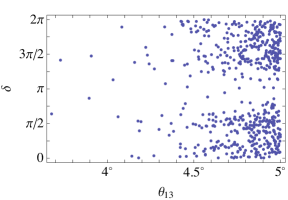
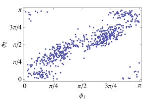
Figure 1: PMNS mixing angles and CP phases in the model close to the best fit values. Shown are the observables obtained by randomly varying the phases of the Yukawa couplings in (27) and (28) while respecting the constraint in (29). Both the solar and the atmospheric mixing angles are within the current $1\sigma$ ranges (see [5]) and the reactor angle is very small, i.e. $\theta_{13}\leq 5^{\circ}$. The Dirac phase $\delta$ (middle panel) and the Majorana phases $\phi_{1}$ and $\phi_{2}$ (right panel) can be large. Interestingly, $\phi_{1}$ and $\phi_{2}$ seem to exhibit a rough correlation $\phi_{1}\simeq\phi_{2}$.

The flavor symmetry group $G_{F}$ is broken at high energies such as the GUT scale. Under renormalization group running from the Planck scale down to low energies, however, the Cabibbo angle $\theta_{\text{C}}$ is essentially stable and $V_{cb}\sim\epsilon^{2}$ changes by a factor less than 2 [43]. Also, since we have a normal hierarchical light neutrino mass spectrum, renormalization group effects have practically no influence on the mass ratios in (33) and change the PMNS mixing angles only by $\ll 1^{\circ}$ (for a discussion and further references see [44]). Given the precision of our model, we therefore neglect the impact of renormalization group effects on our results.

Proton decay via $d=5$ and $d=6$ operators as well as doublet-triplet splitting depend crucially on the geography of the matter fields and on the way in which $SU(5)$ is broken in the extra dimensions (see, e.g., [28, 45]). A detailed study of these issues is therefore beyond the scope of this paper and has to be addressed elsewhere. Moreover, since $G_{F}$ is gauged, one may cancel anomalies by adding Chern-Simons terms in the bulk.

6 Summary and Conclusions

In this paper, we have presented a supersymmetric $SU(5)$ GUT toy model with a discrete non-Abelian flavor symmetry that is broken by Wilson lines. The model is formulated in 4+3 dimensions compactified on a manifold $S^{3}/Z_{n}$. Wilson line breaking of the non-Abelian flavor symmetry is topological and has the advantage that one can have both exact predictions for fermion mixing angles and predictions for the observed fermion mass hierarchies without a vacuum alignment mechanism.

In conjunction with the Froggatt-Nielsen mechanism, the model produces the hierarchical pattern of quark masses and CKM angles. The CKM matrix is entirely generated by the down quark mass matrix which is on a lopsided form, i.e. large atmospheric mixing comes mainly from the charged leptons. In the lepton sector, we obtain the hierarchical charged lepton mass spectrum and normal hierarchical neutrino masses that become small via the type-I seesaw mechanism with three heavy right-handed neutrinos. The PMNS angles are in excellent agreement with current data at $1\sigma$, exhibiting values that could be tested in future neutrino oscillation experiments. The solar angle satisfies the quark-lepton complementarity-type relation $\theta_{12}\approx\pi/4-2\theta_{\text{C}}^{2}$ while the reactor angle is about half the Cabibbo angle. We have shown that the inclusion of nonzero phases of the Yukawa couplings allows large low-energy Dirac and Majorana CP phases. In particular, we have found that the two Majorana phases exhibit a rough correlation $\phi_{1}\sim\phi_{2}$. After Wilson line breaking, the non-Abelian flavor symmetry predicts a maximal atmospheric mixing angle which is driven to larger values by a correction $\sim\theta_{\text{C}}/2$. The simultaneous prediction of (i) nearly maximal atmospheric mixing from the non-Abelian flavor symmetry and (ii) the strict mass hierarchy between the 2nd and 3rd generation of down-type charged fermions is of topological origin: We have non-trivial flavon representations but they can take almost arbitrary VEVs giving practically the same result, i.e. there is no need for a vacuum alignment mechanism.

We have focussed on a specific non-Abelian example flavor symmetry with two-dimensional representations, but it would be desirable to apply flavor symmetry breaking by Wilson lines also to other symmetries such as $A_{4},T^{\prime},$ or $\Delta(3n^{2})$, admitting three-dimensional representations. In this way, one could try to arrive at additional exact predictions for the PMNS mixing angles. Finally, it would also be interesting to see how Wilson line flavor symmetry breaking can be formulated for other GUTs such as $SO(10)$ or $E_{6}$.

References

- [1] N. Cabibbo, Phys. Rev. Lett. 10, 531 (1963); M. Kobayashi and T. Maskawa, Prog. Theor. Phys. 49, 652 (1973).
- [2] B. Pontecorvo, Sov. Phys. JETP 6, 429 (1957); Z. Maki, M. Nakagawa and S. Sakata, Prog. Theor. Phys. 28, 870 (1962).
- [3] H. Georgi and S. L. Glashow, Phys. Rev. Lett. 32, 438 (1974); H. Georgi, in Proceedings of Coral Gables 1975, Theories and Experiments in High Energy Physics, New York, 1975.
- [4] J. C. Pati and A. Salam, Phys. Rev. D 10, 275 (1974) [Erratum-ibid. D 11, 703 (1975)].
- [5] T. Schwetz, M. Tortola and J. W. F. Valle, New J. Phys. 10, 113011 (2008).
- [6] P. F. Harrison, D. H. Perkins and W. G. Scott, Phys. Lett. B 458, 79 (1999); P. F. Harrison, D. H. Perkins and W. G. Scott, Phys. Lett. B 530, 167 (2002).
- [7] E. Ma and G. Rajasekaran, Phys. Rev. D 64, 113012 (2001); K. S. Babu, E. Ma and J. W. F. Valle, Phys. Lett. B 552, 207 (2003); M. Hirsch et al., Phys. Rev. D 69, 093006 (2004).
- [8] P. H. Frampton and T. W. Kephart, Int. J. Mod. Phys. A 10, 4689 (1995); A. Aranda, C. D. Carone and R. F. Lebed, Phys. Rev. D 62, 016009 (2000); P. D. Carr and P. H. Frampton, arXiv:hep-ph/0701034; A. Aranda, Phys. Rev. D 76, 111301 (2007).
- [9] I. de Medeiros Varzielas, S. F. King and G. G. Ross, Phys. Lett. B 648, 201 (2007); C. Luhn, S. Nasri and P. Ramond, J. Math. Phys. 48, 073501 (2007); Phys. Lett. B 652, 27 (2007).
- [10] E. Ma, arXiv:0705.0327 [hep-ph]; G. Altarelli, arXiv:0705.0860 [hep-ph].
- [11] F. Feruglio, C. Hagedorn, Y. Lin and L. Merlo, Nucl. Phys. B 775, 120 (2007).
- [12] M.-C. Chen and K. T. Mahanthappa, Phys. Lett. B 652, 34 (2007); W. Grimus and H. Kuhbock, Phys. Rev. D 77, 055008 (2008); F. Bazzocchi, S. Morisi, M. Picariello and E. Torrente-Lujan, J. Phys. G 36, 015002 (2009); G. Altarelli, F. Feruglio and C. Hagedorn, J. High Energy Phys. 0803, 052 (2008); F. Bazzocchi, M. Frigerio and S. Morisi, arXiv:0809.3573 [hep-ph]; C. Hagedorn, M. A. Schmidt and A. Y. Smirnov, arXiv:0811.2955 [hep-ph].
- [13] G. Cacciapaglia, C. Csaki, C. Grojean and J. Terning, Phys. Rev. D 74, 045019 (2006).
- [14] D. E. Kaplan and T. M. P. Tait, J. High Energy Phys. 0111, 051 (2001).
- [15] K. Agashe, A. Falkowski, I. Low and G. Servant, J. High Energy Phys. 0804, 027 (2008); C. D. Carone, J. Erlich and M. Sher, Phys. Rev. D 78, 015001 (2008).
- [16] F. Plentinger and G. Seidl, Phys. Rev. D 78, 045004 (2008).
- [17] T. Kobayashi, Y. Omura and K. Yoshioka, arXiv:0809.3064 [hep-ph].
- [18] Y. Hosotani, Phys. Lett. B 126, 309 (1983); B 129, 193 (1983).
- [19] P. Candelas, G. T. Horowitz, A. Strominger and E. Witten, Nucl. Phys. B 258, 46 (1985).
- [20] E. Witten, Nucl. Phys. B 258, 75 (1985).
- [21] M. B. Green, J. H. Schwartz, and E. Witten, Superstring theory, volume 2, Cambridge University Press, Cambridge (1987).
- [22] L. E. Ibanez, H. P. Nilles and F. Quevedo, Phys. Lett. B 187, 25 (1987); B 192, 332 (1987).
- [23] L. J. Hall, H. Murayama and Y. Nomura, Nucl. Phys. B 645, 85 (2002).
- [24] L. M. Krauss and F. Wilczek, Phys. Rev. Lett. 62, 1221 (1989).
- [25] E. Witten, arXiv:hep-ph/0201018.
- [26] R. Barbieri, G. R. Dvali and A. Strumia, Phys. Lett. B 333, 79 (1994).
- [27] G. G. Ross, arXiv:hep-ph/0411057.
- [28] Y. Kawamura, Prog. Theor. Phys. 105, 999 (2001); G. Altarelli and F. Feruglio, Phys. Lett. B 511, 257 (2001); A. B. Kobakhidze, Phys. Lett. B 514, 131 (2001); A. Hebecker and J. March-Russell, Nucl. Phys. B 613, 3 (2001); L. J. Hall and Y. Nomura, Phys. Rev. D 66, 075004 (2002).
- [29] P. Minkowski, Phys. Lett. B 67, 421 (1977); T. Yanagida, in Proceedings of the Workshop on the Unified Theory and Baryon Number in the Universe, KEK, Tsukuba, 1979; M. Gell-Mann, P. Ramond and R. Slansky, in Proceedings of the Workshop on Supergravity, Stony Brook, New York, 1979; S. L. Glashow, in Proceedings of the 1979 Cargese Summer Institute on Quarks and Leptons, New York, 1980.
- [30] M. Magg and C. Wetterich, Phys. Lett. B 94, 61 (1980); R. N. Mohapatra and G. Senjanović, Phys. Rev. Lett. 44, 912 (1980); Phys. Rev. D 23, 165 (1981); J. Schechter and J. W. F. Valle, Phys. Rev. D 22, 2227 (1980); G. Lazarides, Q. Shafi and C. Wetterich, Nucl. Phys. B 181, 287 (1981).
- [31] D. Gorenstein, Finite Simple Groups; An Introduction to Their Classification, Plenum, New York (1983); The Classification of the Finite Simple Groups, Volume I, Plenum, New York (1983).
- [32] H. Kurzweil and B. Stellmacher, Theorie der endlichen Gruppen: eine Einführung, Springer, Berlin (1998).
- [33] A. Y. Smirnov, arXiv:hep-ph/0402264; M. Raidal, Phys. Rev. Lett. 93, 161801 (2004); H. Minakata and A. Y. Smirnov, Phys. Rev. D 70, 073009 (2004).
- [34] F. Plentinger, G. Seidl and W. Winter, JHEP 0804, 077 (2008).
- [35] C. D. Froggatt and H. B. Nielsen, Nucl. Phys. B 147, 277 (1979).
- [36] C. Csaki, C. Grojean and H. Murayama, Phys. Rev. D 67, 085012 (2003).
- [37] C. H. Albright, K. S. Babu and S. M. Barr, Phys. Rev. Lett. 81, 1167 (1998).
- [38] H. Georgi and C. Jarlskog, Phys. Lett. B86, 297 (1979).
- [39] S. Niehage and W. Winter, arXiv:0804.1546 [hep-ph].
- [40] P. Huber, J. Kopp, M. Lindner, M. Rolinec and W. Winter, JHEP 05, 072 (2006).
- [41] D. S. Ayres et al. [NOA Collaboration], arXiv:hep-ex/0503053; Y. Hayato et al., Letter of Intent.
- [42] F. Deppisch, F. Plentinger, W. Porod, R. Ruckl, and G. Seidl, in preparation.
- [43] H. Arason et al., Phys. Rev. Lett. 67, 2933 (1991); H. Arason et al., Phys. Rev. D 47, 232 (1993).
- [44] F. Plentinger, G. Seidl and W. Winter, Phys. Rev. D 76, 113003 (2007).
- [45] K. Kurosawa, N. Maru and T. Yanagida, Phys. Lett. B 512, 203 (2001).