Reiter’s Polaron Wavefunction Applied
to a $t_{2g}$ Orbital $t$–$J$ Model

Abstract

Using the self-consistent Born approximation we calculate Reiter’s wavefunction for a single hole introduced into the undoped and orbitally ordered ground state of the $t$–$J$ model with $t_{2g}$ orbital degrees of freedom. While the number of excitations is similar to the spin $t$-$J$ model for a given $J/t$, a distinct structure of the calculated wavefunction and its momentum dependence is identified suggesting the formation of a novel type of mobile polarons.

Introduction— Recently, using self-consistent Born approximation (SCBA), we showed that a single hole introduced into the undoped ground state of an orbital $t$–$J$ model with $t_{2g}$ orbital degeneracy propagates coherently as a quasiparticle [1]. This striking result contradicts the naïve expectations which suggest that a hole should be trapped in this Ising-like ordered ground state. In fact, the motion of a single hole is due to the frequently neglected three-site terms and we showed [1] that this new mechanism of hole movement is fundamentally different from the coherent hole motion via quantum fluctuations in the standard spin $t$–$J$ model [2], or in the case of $e_{g}$ orbitals [3]. Though, a more detailed understanding of this novel mechanism is needed. Hence, instead of considering the Green’s function of the problem [1], we investigate the corresponding Reiter’s wavefunction [4] calculated in the SCBA.

Orbital polarons— The orbital $t$–$J$ Hamiltonian, relevant for ferromagnetic $ab$ planes with two active $t_{2g}$ orbitals, $zx\equiv b$ and $yz\equiv a$, at each site, consists of three terms [1] ${\mathcal{H}}={\mathcal{H}}_{t}+{\mathcal{H}}_{J}+{\mathcal{H}}_{3s}$, with

$${\mathcal{H}}_{t}= -t\sum_{i}\left(\tilde{b}^{\dagger}_{i}\tilde{b}_{i+\bf{\hat{x}}}+\tilde{a}^{\dagger}_{i}\tilde{a}_{i+\bf{\hat{y}}}+h.c.\right),$$ (1a)

$${\mathcal{H}}_{J}= \;\frac{1}{2}J\sum_{\langle ij\rangle}\left(T^{z}_{i}T^{z}_{j}-\frac{1}{4}\tilde{n}_{i}\tilde{n}_{j}\right),$$ (1b)

$${\mathcal{H}}_{\rm 3s}= -\frac{1}{4}J\sum_{i}\left(\tilde{b}^{\dagger}_{i-\bf{\hat{x}}}\tilde{n}_{ia}\tilde{b}_{i+\bf{\hat{x}}}+\tilde{a}^{\dagger}_{i-\bf{\hat{y}}}\tilde{n}_{ib}\tilde{a}_{i+\bf{\hat{y}}}+h.c.\right),$$ (1c)

where a tilde above fermion operators denote the restricted Hilbert space without double occupancies, the total on-site density $\tilde{n}_{i}=\tilde{n}_{ia}+\tilde{n}_{ib}=\tilde{a}^{\dagger}_{i}\tilde{a}_{i}+\tilde{b}^{\dagger}_{i}\tilde{b}_{i}$, and the pseudospin operators $T^{z}_{i}=\frac{1}{2}(\tilde{n}_{ib}-\tilde{n}_{ia})$. In Eq. (1c) we neglected the three-site terms which require orbital excitation and therefore do not change the physical properties of the system in the low doping regime (cf. discussion in Ref. [1]).

Following Ref. [2] we reduce the $t$–$J$ model to a polaronic problem, which is a physically justified procedure for the AF or AO ordered phases with low concentration of added holes [5]. Hence, we: (i) divide the square lattice into two sublattices $A$ and $B$, (ii) rotate pseudospins on the $A$ sublattice, and (iii) introduce fermion operators $h^{\dagger}_{i}$ and hard-core boson operators $\alpha^{\dagger}_{i}$ such that $\tilde{a}_{i}=h_{i}^{\dagger}\alpha_{i}$ and $\tilde{b}_{i}=h_{i}^{\dagger}(1-\alpha_{i}^{\dagger}\alpha_{i})$. Then, in the linear spin-wave approximation and having only one doped hole in the plane, we obtain the following Fourier-transformed polaronic Hamiltonian, $H=H_{t}+H_{J}+H_{3s}$, with

$$H_{t}\!= \frac{1}{\sqrt{N}}\!\sum_{{\bf k},{\bf q}}\!\left[M_{x}({\bf k},\!{\bf q})h^{\dagger}_{{\bf k}A}h_{{\bf k}-{\bf q}B}\alpha_{{\bf q}A}\!\!+\!M_{y}({\bf k},\!{\bf q})h^{\dagger}_{{\bf k}B}h_{{\bf k}-{\bf q}A}\alpha_{{\bf q}B}\!+\!h.c.\right]\!,$$ (2a)

$$H_{J}\!= \;\omega_{0}\sum_{\bf k}\left(\alpha_{{\bf k}A}^{\dagger}\alpha_{{\bf k}A}+\alpha_{{\bf k}B}^{\dagger}\alpha_{{\bf k}B}\right),$$ (2b)

$$H_{\rm 3s}\!= \;\sum_{\bf k}\left[\varepsilon_{y}({\bf k})h_{{\bf k}A}^{\dagger}h_{{\bf k}A}\!+\!\varepsilon_{x}({\bf k})h_{{\bf k}B}^{\dagger}h_{{\bf k}B}\right].$$ (2c)

Here the sums go over all momenta $\{{\bf k}\}$ in the Brillouin zone for the whole lattice, the total number of sites is $N$, and the orbiton energy is $\omega_{0}=J$.

The vertices and the dispersion relations are equal to (with $\nu=x,y$):

$$M_{\nu}({\bf k},{\bf q})=2t\cos(k_{\nu}-q_{\nu}),\hskip 48.36958pt\varepsilon_{\nu}({\bf k})=\textstyle{\frac{1}{2}}J\cos(2k_{\nu}).$$ (3)

Reiter’s wavefunction— In the spirit of Ref. [4], let us assume that the wavefunction for a hole with quasiparticle (QP) momentum ${\bf k}$ and initially doped into the sublattice $A$ and $B$, respectively, takes the form:

$$|\Psi_{{\bf k}A}\rangle= \;a^{(0)}_{A}({\bf k})h^{\dagger}_{{\bf k}A}|0\rangle+\frac{1}{\sqrt{N}}\sum_{\bf q}a^{(1)}_{A}({\bf k},{\bf q})h^{\dagger}_{{\bf k}-{\bf q}B}\alpha_{{\bf q}A}^{\dagger}|0\rangle$$

$$+ \;\frac{1}{N}\sum_{{\bf q}_{1},{\bf q}_{2}}a^{(2)}_{A}({\bf k},{\bf q}_{1},{\bf q}_{2})h^{\dagger}_{{\bf k}-{\bf q}_{1}-{\bf q}_{2}A}\alpha_{{\bf q}_{1}A}^{\dagger}\alpha_{{\bf q}_{2}B}^{\dagger}|0\rangle+\cdots\ ,$$ (4a)

$$|\Psi_{{\bf k}B}\rangle= \;a^{(0)}_{B}({\bf k})h^{\dagger}_{{\bf k}B}|0\rangle+\frac{1}{\sqrt{N}}\sum_{\bf q}a^{(1)}_{B}({\bf k},{\bf q})h^{\dagger}_{{\bf k}-{\bf q}A}\alpha_{{\bf q}B}^{\dagger}|0\rangle$$

$$+ \;\frac{1}{N}\sum_{{\bf q}_{1},{\bf q}_{2}}a^{(2)}_{B}({\bf k},{\bf q}_{1},{\bf q}_{2})h^{\dagger}_{{\bf k}-{\bf q}_{1}-{\bf q}_{2}B}\alpha_{{\bf q}_{1}B}^{\dagger}\alpha_{{\bf q}_{2}A}^{\dagger}|0\rangle+\cdots\ .$$ (4b)

The coefficients $\Big{|}a^{(0)}_{L}({\bf k})\Big{|}^{2}$ (with the sublattice index $L\in\{A,B\}$) are the QP spectral weights which follow from the normalization of the wavefunction, whereas $a^{(n)}_{L}({\bf k},{\bf q}_{1},...,{\bf q}_{n})$ for $n>0$ are to be determined from the Schrödinger equations $H|\Psi_{{\bf k}L}\rangle=\lambda_{{\bf k}L}|\Psi_{{\bf k}L}\rangle$. Substituting Eq. (4)–(4) into them yields

$$a^{(2n)}_{A}\!({\bf k}\!,\!\{{\bf q}_{i}\}_{2n})\!\!\! \!\!\!=\!\!\! \!\!\!a^{(2n-1)}_{A}\!({\bf k},\!\{{\bf q}_{i}\}_{2n\!-\!1})\!M_{y}\!(\bar{{\bf k}}_{2n\!-\!1}\!,\!{\bf q}_{2n})G_{A}(\bar{{\bf k}}_{2n},\!\mu^{(2n)}_{{\bf k}A}),$$ (5a)

$$a^{(2n-1)}_{A}({\bf k},\!\{{\bf q}_{i}\}_{2n\!-\!1})\!\!\! \!\!\!=\!\!\! \!\!\!a^{(2n\!-\!2)}_{A}\!({\bf k},\!\!\{{\bf q}_{i}\}_{2n\!-\!2}\!)M_{x}(\bar{{\bf k}}_{2n\!-\!2},{\bf q}_{2n\!-\!1})G_{B}(\bar{{\bf k}}_{2n\!-\!1},\mu^{(2n\!-\!1)}_{{\bf k}A}),$$

$$a^{(2n)}_{B}\!({\bf k}\!,\!\{{\bf q}_{i}\}_{2n})\!\!\! \!\!\!=\!\!\! \!\!\!a^{(2n-1)}_{B}\!({\bf k},\!\{{\bf q}_{i}\}_{2n\!-\!1})\!M_{x}\!(\bar{{\bf k}}_{2n\!-\!1}\!,\!{\bf q}_{2n})G_{B}(\bar{{\bf k}}_{2n},\!\mu^{(2n)}_{{\bf k}B}),$$ (5c)

$$a^{(2n-1)}_{B}({\bf k},\!\{{\bf q}_{i}\}_{2n\!-\!1})\!\!\! \!\!\!=\!\!\! \!\!\!a^{(2n\!-\!2)}_{B}\!({\bf k},\{{\bf q}_{i}\}_{2n\!-\!2})M_{y}(\bar{{\bf k}}_{2n\!-\!2},{\bf q}_{2n\!-\!1})G_{A}(\bar{{\bf k}}_{2n\!-\!1},\mu^{(2n\!-\!1)}_{{\bf k}B}),$$

where $\bar{\bf k}_{n}={\bf k}-{\bf q}_{1}-...-{\bf q}_{n}$, $\{{\bf q}_{i}\}_{n}=\{{\bf q}_{1},{\bf q}_{2},...,{\bf q}_{n}\}$, $\mu^{(n)}_{{\bf k}L}=\lambda_{{\bf k}L}-n\omega_{0}$. The Green’s functions $G_{L}$ are defined by the self-consistent equations

$$G^{-1}_{A}({\bf k},\omega) =\omega-\varepsilon_{y}({\bf k})-\frac{1}{N}\sum_{\bf q}G_{B}({\bf k}-{\bf q},\omega-\omega_{0})M_{x}^{2}({\bf k},{\bf q})\ ,$$ (6a)

$$G^{-1}_{B}({\bf k},\omega) =\omega-\varepsilon_{x}({\bf k})-\frac{1}{N}\sum_{\bf q}G_{A}({\bf k}-{\bf q},\omega-\omega_{0})M_{y}^{2}({\bf k},{\bf q})\ ,$$ (6b)

and the QP energy has to be equal

$$\lambda_{{\bf k}A} = \varepsilon_{y}({\bf k})+\frac{1}{N}\sum_{\bf q}G_{B}({\bf k}-{\bf q},\mu^{(1)}_{{\bf k}A})M_{x}^{2}({\bf k},{\bf q})\ ,$$ (7a)

$$\lambda_{{\bf k}B} = \varepsilon_{x}({\bf k})+\frac{1}{N}\sum_{\bf q}G_{A}({\bf k}-{\bf q},\mu^{(1)}_{{\bf k}B})M_{y}^{2}({\bf k},{\bf q})\ .$$ (7b)

Note, that in order to obtain equations for the coefficients of the Reiter’s wavefunction $a^{(n)}_{L}$ Eqs. (5) we adopted the following contraction procedure: we neglected all terms which would correspond to the annihilation of orbitons in the $n$-th step if the orbitons were created earlier than in the $(n-1)$-th step. This procedure resembles the non-crossing approximation while calculating Green’s function using the diagrammatic technique. In fact, one may wonder why we still have to adopt such approximation since the closed loops which correspond to the crossing diagrams are anyway prohibited in the orbital $t$–$J$ model under consideration [1]. The answer to this puzzle is the following: to conclude that the crossing diagrams are unphysical we not only need to look at the structure of the Hamiltonian Eq. (2) but also at the processes allowed by this Hamiltonian on the square lattice. Thus, we need some extra information about the lattice to exclude the crossing diagrams, and consequently we need to introduce the contraction procedure by hand.

Consequences— Eqs. (5) together with Eqs. (6) and (7) can be easily solved numerically. While it is impossible to calculate the coefficients $a^{(n)}_{L}$ for all $n$, one may ask whether there exists such an $m$ that all the coefficients with $n>m$ are so small that they could be safely neglected. This question is also of physical importance since knowing $m$ would mean that the wavefunction of the doped hole can be approximated by a superposition of the wavefunction of a free hole and $m$ wavefunctions of the hole dressed with $m$ orbitons.

The easiest way to answer the above question is to calculate the norm

$$N_{{\bf k}A}\equiv\langle\Psi_{{\bf k}A}|\Psi_{{\bf k}A}\rangle=\Big{|}a^{(0)}_{A}({\bf k})\Big{|}^{2}\Big{\{}1+\frac{1}{N}\sum_{{\bf q}_{1}}|M_{x}({\bf k},{\bf q}_{1})G_{B}(\bar{\bf k}_{1},\mu^{(1)}_{{\bf k}A})|^{2}$$

$$+\frac{1}{N^{2}}\sum_{{\bf q}_{1},{\bf q}_{2}}|M_{x}({\bf k},{\bf q}_{1})G_{B}(\bar{{\bf k}}_{1},\mu^{(1)}_{{\bf k}A})|^{2}|M_{y}(\bar{{\bf k}}_{1},{\bf q}_{2})G_{A}(\bar{{\bf k}}_{2},\mu^{(2)}_{{\bf k}A})|^{2}$$

$$+\frac{1}{N^{3}}\sum_{{\bf q}_{1},{\bf q}_{2},{\bf q}_{3}}|M_{x}({\bf k},{\bf q}_{1})G_{B}(\bar{{\bf k}}_{1},\mu^{(1)}_{{\bf k}A})|^{2}|M_{y}(\bar{{\bf k}_{1}},{\bf q}_{2})G_{A}(\bar{{\bf k}}_{2},\mu^{(2)}_{{\bf k}A})|^{2}$$

$$\hskip 8.5359pt|M_{x}(\bar{{\bf k}}_{2},{\bf q}_{3})G_{B}(\bar{{\bf k}}_{3},\mu^{(3)}_{{\bf k}A})|^{2}+\cdots\Big{\}}\equiv N_{{\bf k}A}^{(0)}\!+\!N_{{\bf k}A}^{(1)}\!+\!N_{{\bf k}A}^{(2)}\!+\!N_{{\bf k}A}^{(3)}\!+\cdots\ ,$$ (8)

of the wavefunction on the $A$ sublattice given by Eq. (4), and similarly $N_{{\bf k}B}$ for the $B$ sublattice. Naturally, $N_{{\bf k}L}=1$ which yields the following suggestion: If the sum of the norms of the $m$ first terms of the wavefunction fulfills the equation $\sum_{n=0}^{m}N^{(n)}_{{\bf k}L}\cong 1$, then all terms with $n>m$ in the Reiter’s wavefunction can be neglected.

In order to deduce what is the value of $m$ for different values of the orbiton energy $J$ we calculated numerically $N^{(n)}_{{\bf k}L}$ for $n=0,1,2,3$ as a function of $J$ on a mesh of $16\times 16$ $k$ points , cf. Fig. 1. The obtained results do not depend on the sublattice index $L$. Fig. 1(a) shows the results for the orbital model Eq. (2a)–(2b) whereas Fig. 1(b) shows the results for the orbital model Eq. (2a-2c). We conclude that: ($i$) for both cases for $J\gtrsim 0.4t$ the norm of the wavefunction is close to $1$ already for $m=3$ and hence there are just up to three orbitons participating in the formation of a polaron, ($ii$) it seems that only few more orbitons are excited for smaller $J$, and ($iii$) for the case with three-site terms $N^{(n)}_{{\bf k}L}$ depends slightly on the momentum ${\bf k}$ — it follows the dependence of the QP spectral weight $N^{(0)}_{{\bf k}L}\equiv\Big{|}a^{(0)}_{L}({\bf k})\Big{|}^{2}$ on ${\bf k}$, with a maximum at ${\bf k}=(\pi/2,\pi/2)$, i.e. at the minimum of $\varepsilon({\bf k})$, cf. Eq. (3), and ($iv$) the dependence of $N^{(n)}_{{\bf k}L}$ on ${\bf k}$ found only when the three-site terms are included demonstrates that the three-site terms are indeed responsible for the formation of mobile polarons.

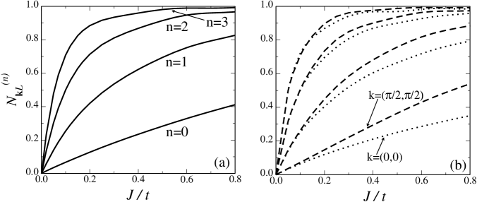
Fig. 1: The norm $N^{(n)}_{{\bf k}L}$ as a function of $J$ for $n=0,1,2,3$, from bottom to top respectively, as obtained for the orbital model (a) without and (b) with three-site terms Eq. (2c) included in the Hamiltonian. The results on panel (a) do not depend on ${\bf k}$ whereas dotted (dashed) lines on panel (b) show results for ${\bf k}=(0,0)$ [${\bf k}=(\pi/2,\pi/2)$], respectively. All of the results do not depend on the sublattice index $L$.

Summary— As a summary, it is instructive to compare the results of the realistic orbital $t$–$J$ model (i.e. with three-site terms included) with those obtained for the spin Ising model and for the spin SU(2) symmetric model in Refs. [6]-[7]. On one hand, for all $n$ the dependence of the norm $N^{(n)}_{{\bf k}L}$ on ${\bf k}$ resembles to some extent the spin SU(2) model. On the other hand, a closer look reveals that even for ${\bf k}=(0,0)$ the dependence of $N^{(n)}_{{\bf k}L}$ on $J$ is a concave function for all $n$ just as for the spin Ising case and unlike in the $SU(2)$ case where it can be a convex function of $J$ for some $n$ [7]. Hence, the detailed study of the Reiter’s vavefunction of the orbital polaron confirms that the hole doped into the $t_{2g}$ AO forms a mobile polaron just like the mobile spin polaron in the AF plane of high-$T_{c}$ cuprates [2] but its properties are truly distinct, in agreement with discussion in Ref. [1].

References

• [1] M. Daghofer, K. Wohlfeld, A.M. OleΕ›, E. Arrigoni, and P. Horsch, Phys. Rev. Lett. 100, 066403 (2008).
• [2] G. MartΓ­nez and P. Horsch, Phys. Rev. B 44, 317 (1991).
• [3] J. van den Brink, P. Horsch, and A.M. OleΕ›, Phys. Rev. Lett 85, 5174 (2000).
• [4] G.F. Reiter, Phys. Rev B 49, 1536 (1994).
• [5] M. Brunner, F.F. Assaad, and A. Muramatsu, Phys. Rev. B 62, 15480 (2000).
• [6] P. Horsch and A. RamΕ‘ak, J. Low Temp. Phys. 95, 343 (1994).
• [7] A. RamΕ‘ak and P. Horsch, Phys. Rev. B 57, 4308 (1998).