Spectral properties of orbital polarons in Mott insulators

Abstract

We address the spectral properties of Mott insulators with orbital degrees of freedom, and investigate cases where the orbital symmetry leads to Ising-like superexchange in the orbital sector. The paradigm of a hole propagating by its coupling to quantum fluctuations, known from the spin $t$–$J$ model, then no longer applies. We find instead that when one of the two orbital flavors is immobile, as in the Falicov-Kimball model, trapped orbital polarons coexist with free hole propagation emerging from the effective three-site hopping in the regime of large on-site Coulomb interaction $U$. The spectral functions are found analytically in this case within the retraceable path approximation in one and two dimensions. On the contrary, when both of the orbitals are active, as in the model for $t_{2g}$ electrons in two dimensions, we find propagating polarons with incoherent scattering dressing the moving hole and renormalizing the quasiparticle dispersion. Here, the spectral functions, calculated using the self-consistent Born approximation, are anisotropic and depend on the orbital flavor. Unbiased conclusions concerning the spectral properties are established by comparing the above results for the orbital $t$–$J$ models with those obtained using the variational cluster approximation or exact diagonalization for the corresponding Hubbard models. The present work makes predictions concerning the essential features of photoemission spectra of certain fluorides and vanadates.

I Introduction

A hole propagates coherently in the valence band of a band insulator with an unrenormalized one-particle dispersion (i.e., determined by electronic structure calculations), whereas hole propagation in a Mott insulator is a nontrivial many-body problem. The paradigm here is a hole doped in the half filled one-band Hubbard model that is a minimal model used to describe the parent compounds of high-$T_{c}$ superconductors. Such a hole forms a defect in the antiferromagnetic (AF) background, and its coherent propagation may appear then only on a strongly renormalized energy scale.Ima98 Naively, i.e., considering the Néel state induced by Ising-like spin interactions, one expects that a propagating hole would disturb the AF background and generate a string of broken bonds, with ever increasing energy cost when the hole creates defects moving away from its initial position. This suggests hole confinement as realized already four decades ago.Bul68 Nevertheless, the quantum nature of this problem leads to a new quality: a hole in the AF Mott insulator can propagate coherently on the energy scale $J$ which controls AF quantum fluctuations, Sch89 ; Kan89 ; Mar91 because they heal the defects arising on the hole path. Crucial for this observation is the presence of transverse spin components $\propto(S_{i}^{+}S_{j}^{-}+S_{i}^{-}S_{j}^{+})$, responsible for quantum fluctuations in the SU(2)-symmetric Heisenberg exchange interactions.

In contrast, the orbital interactions which induce alternating orbital (AO) order are known to be more Ising-likevdB04 (classical) and quantum fluctuations are then either substantially reduced,vdB99 or even absent. Perhaps the most prominent example of robust orbital order occurs for degenerate $e_{g}$ orbitals in the ferromagnetic (FM) planes of LaMnO₃.Dag01 Orbital interactions are there induced both by the lattice (due to cooperative Jahn-Teller effect) and by the superexchangeFei99 — both of them are classical and Ising-like, so the quantum fluctuations are to a large extent suppressed. Therefore, the orbital order is more robust than the spin order in two-dimensional (2D) models,Dag07 and a higher hole concentration is required to destroy it.Hor99 In the three-dimensional case off-diagonal (interorbital) hopping ($e_{g}$ orbital flavor is here not conservedZaa93 ) may even lead to an orbital liquid phase already at rather low hole doping.Fei05

Another difference to the SU(2) spin model is that a hole in a ferromagnet with AO order of $e_{g}$ orbitals can propagate coherently without introducing any string states. This coherent propagation arises here due to the $e_{g}$ interorbital hopping, but is strongly renormalized by orbital excitations.vdB00 However, in the $t_{2g}$ systems the interorbital hopping is forbidden by symmetry,Zaa93 and the superexchange is purely Ising-like, so the above established mechanisms of coherent hole propagation in the regime of large on-site Coulomb repulsion $U$, i.e., for $t\ll U$ where $t$ is the hopping element, are absent. One may then wonder whether a hole doped to a Mott insulator with the $t_{2g}$ AO order would then be confined.Dag08

The present paper is motivated by the above important difference between the spin physics and the orbital physics, especially prominent in the hole motion in the $t_{2g}$ orbital systems. Dag08 In spin models, the Ising-like superexchange represents only a rather poor approximation for the SU(2)-symmetric Heisenberg spin exchange (as obtained in the $t$-$J$ model by its derivation from the Hubbard model Cha77 ) and could merely serve as a starting point for the full SU(2)-symmetric calculations. Wro08 In contrast, in the systems with $t_{2g}$ orbital degeneracy the Ising superexchange follows from a similar derivation as an accurate description of charge excitations in the second order of the perturbation theory in the regime of $t\ll U$, in cases when only two orbitals are active (see below). Strictly speaking, in these realistic orbital systems the Ising-like superexchange occurs in a two-band model when precisely one orbital flavor permits the hopping along each bond, as only then the orbital flavor cannot be exchanged and the pseudospin $(T^{+}_{i}T^{-}_{j}+T^{-}_{i}T^{+}_{j})$ operators are absent in the respective $t$–$J$ model.noteti Such a situation is found not only in the above mentioned $t_{2g}$ model but also in three other distinct orbital models (see below). Hence, in the following paragraphs we give a brief overview of these four models with realistic Ising superexchange for which the spectral function of a single hole doped into the half-filled ground state will be studied in this paper.

As a first example we introduce the spinless Falicov-Kimball (FK) model which describes itinerant $d$ electrons coupled to localized $f$ electrons. On sites occupied by an $f$ electron, the $d$ electrons feel a strong on-site Coulomb repulsion $U$. The FK model can be solved exactly in infinite dimension,Fre03 where it leads to a complex phase diagram including periodic ground states as well as a regime of phase separation. When the energies of two involved orbitals are degenerate (which is not the case in $4f$ or $5f$ materials), one finds that electron densities in the two orbitals are the same ($n_{d}=n_{f}$), and second order perturbation theory leads in the regime of large $U$ to a strong-coupling model with one mobile flavor. One finds therefore the ground state with the AO order formed by sites occupied by $d$ and $f$ electrons on the two sublattices. The spectral density for the mobile $d$ electrons can be obtained as well in one Bec07 and two dimensions,Mas06 but computation of the $f$ spectral density is quite involved even at infinite dimension. Fre05 Below we will discuss exact one-dimensional (1D) and approximate two-dimensional (2D) analytic results for the relevant FK models.

A second and different realization of the effective low-energy model with Ising superexchange was proposed recentlyDag08 for FM planes in transition metal oxides with $t_{2g}$ orbital degeneracy: In this case, both orbital flavors are equivalent (the third one is inactive) and both allow for electronic hopping, however, each one permits the hopping along one axis only. Despite the 1D character of the kinetic energy in such a model, the ground state at half filling has 2D AO order, stabilized by the Ising superexchange. Electron propagation, on the other hand, is strictly 1D, so a hole replacing an electron with either orbital flavor may only move in one direction by the hopping $t$. Such a situation might be realized in Sr₂VO₄, where the crystal field splits the $t_{2g}$ orbitals Mat05 and one finds indeed AO orderIma05 in the weakly FM planes. Noz91 A different possible realization of such a model is found in cold-atom systems,Jan05 with strongly anisotropic hopping in the spinless $p$-orbital Hubbard model.p_Hubb

The third realization concerns systems with peculiar $e_{g}$ AO and is somewhat subtle. As described above in the ”well-known” systems with active $e_{g}$ orbitals (such as the perovskite manganites) the hole can propagate coherently due to the interorbital hopping.Fei05 However, one can identify two peculiar cases of $e_{g}$ AO order where the interorbital hopping is strongly reduced between the orbitals occupied in the ground state, and the question of the hole confinement in the Ising superexchange model is of high relevance. The first one is realized in the FM planes of K₂CuF₄,Hid83 or in the recently investigated Cs₂AgF₄.Wu07 While the AO order is formed in these cases by $e_{g}$ orbitals, crystal field stabilizes their particular linear combinations with alternating $x^{2}-z^{2}/y^{2}-z^{2}$ $e_{g}$ orbitals,McL06 and thus suppresses the interorbital hopping present, for instance, in the ground state of the manganites. In addition, the phase factors of two orbitals along each bond allow for the hopping only along one direction in the plane, Zaa93 so one arrives at a situation similar to that found for strongly correlated electrons in $t_{2g}$ orbitals — it will be discussed in the Appendix A. Thus, the model called $t_{2g}$ model throughout this paper is expected to describe a wider class of transition metal oxides.

Finally, another case where the AO order could in principle lead to the hole confinement is the situation encountered in the 1D $e_{g}$ model in which the interorbital hopping and quantum fluctuations are suppressed by symmetry. Since this model is actually equivalent to the 1D FK model discussed above, we will refer to it later simply as to the ”1D model”. Its study was stimulated by the experimental findings in the lightly hole-doped vanadates such as La_1-xSr_xVO₃.Fuj08 There the ground state for $x=0.1$ is an insulating three-dimensional FM phase with AO order at $x=0.10$. The physical origin of the Mott insulating state in the case of such a finite hole doping is not yet understood. Again, a natural question could be whether the peculiar stability of the Mott insulating state is related to the presence of the AO order. Since it is obvious that the hole can move in the AO state in the plane (due to the interorbital hopping, see above) it is interesting to verify whether the AO order along the third direction could block the hole motion.

The four above cases are, to our knowledge, the only straightforward models in which the full superexchange is purely classical, i.e., where Ising superexchange follows from the orbital symmetry, and is not an approximation to the Heisenberg Hamiltonian.Poi04 The superexchange models, however, have to be extended by the second order three-site hopping terms in each case. Such effective hopping terms arise in the same order of the perturbation theory when holes are present, and are necessary for a faithful representation of the spectral weight distribution in the one-particle and in the optical spectra of the underlying spin Hubbard model.Esk94 Therefore, also in the present orbital $t$-$J$ models with Ising superexchange similar terms are expected to play an important role and cannot be neglected. Moreover, while in the spin case such terms are in conflict with the quantum fluctuations and give thus only minor quantitative corrections to the coherent hole motion, vSz90 in the orbital (pseudospin) models with Ising superexchange they become of crucial importance as they are the only possible source for coherent carrier propagation (the Trugman loopsTru88 with the hole repairing the defects on its path are here absent) and dictate possible coherent processes.Dag08 To get a better understanding of the balance between the coherent and incoherent processes in the orbital strong-coupling models (i.e. $t$-$J$ models with three-site terms) we analyze their spectral properties in some detail below.

In order to arrive at a comprehensive and rather complete understanding of the elemental processes which accompany hole propagation in the orbital models, we not only combine numerical and analytical approaches but also we calculate the spectral properties both of the strong-coupling and of the respective Hubbard models. Hence, we first determine the Green’s functions using the self-consistent Born approximation (SCBA) and the analytical treatments applied to the above mentioned orbital strong-coupling models. This allows us to identify the dominant mechanism responsible for the quasiparticle (QP) behavior. We note that for finite doping such methods as the slave boson approach, the path integral formalism, or the numerical approaches, are much more suitable for the $t$-$J$-like models than the SCBA.Gre06 However, in the one hole limit the SCBA gives reasonably good results which are in agreement with other methods.Mar91 ; Gre06 . We then compare these results to those obtained for the respective orbital Hubbard model. Here, in some cases we determine Green’s functions numerically by use of exact diagonalization on small clusters, in others we use the variational cluster approach (VCA),Aic03 where a cluster is solved exactly and then embedded into a larger system. This variational approach is based on cluster perturbation theory developed in the last decade,Gro93 ; Mas98 ; Sen00 and corresponds to taking the self-energy from a small cluster and optimizing it with respect to mean-field terms arising due to the AO order. The embedding via the self-energy approachPot03 allows us to include long-range (orbital) ordering phenomena by optimizing a fictitious field due to the AO order. This method is appropriate for orbital Hubbard models with on-site interactions. Since the exact solution on the cluster is obtained for the full Hamiltonian, it contains all potentially relevant processes like, e.g., the three-site hopping.

The paper is organized as follows. The 1D orbital model is introduced in Sec. II whereas its extension to the 2D FK model is discussed in Sec. III. In both sections, we introduce the respective Hubbard-like Hamiltonian, derive from it the appropriate strong-coupling Hamiltonian, and calculate analytically the hole Green’s function for the AO state at half filling. Next, we introduce an exactly-solvable 1D model with three-atom units along the chain (Sec. IV), called the 1D ’centipede’ model. The latter model (which was not mentioned above) serves merely as a didactic tool and explains the essence of string excitations present in the 2D model with $t_{2g}$ orbital flavors, discussed thoroughly in Sec. V. Here, again we start from the orbital Hubbard model, derive its strong-coupling version, and calculate the hole Green’s function for the AO state at half filling, using two approximate methods described above: the SCBA and the VCA. In Sec. VI we include longer-range hopping in the 2D $t_{2g}$ model (as expected in real materials) and discuss the main experimental implications of our study by calculating the photoemission spectra of certain vanadates and fluorides. General conclusions are presented in Sec. VII. The analysis is supplemented by the Appendix A, where we derive the effective strong-coupling model for the above mentioned fluorides and prove that the $t_{2g}$ model discussed in Sec. V may indeed be applied to the hole motion in the systems with a particular type of $e_{g}$ orbital order.

II 1D orbital model with Ising superexchange

II.1 Effective strong-coupling model

As explained in Sec. I, the Ising-like superexchange follows if only one orbital flavor permits hopping along each bond, and the spins are polarized in the FM state. The simplest case which captures the essential features of the effective strong-coupling model with Ising-like superexchange follows from the 1D orbital Hubbard model

$$H_{\rm 1D}=-t\sum_{i}(a^{\dagger}_{i}a_{i+1}+\textrm{h.c.})+U\sum_{i}n_{ia}n_{ib}\;,$$ (1)

where $a^{\dagger}_{i}$ ($b^{\dagger}_{i}$) creates a spinless electron with orbital flavor $a$ ($b$) at site $i$, and $\{n_{ia},n_{ib}\}$ are electron density operators. On-site Coulomb repulsion $U$ is the energy of a doubly occupied state (it arises as a linear combination of the Coulomb and Hund’s exchange in the respective high-spin configurationvdB99 ), and $t$ is the nearest neighbor (NN) hopping element. Only electrons with orbital flavor $a$ are mobile while the other ones with flavor $b$ cannot hop. To simplify, we call below the $a$ and $b$ orbitals mobile and immobile ones, respectively. This situation corresponds to (spinless) interacting $e_{g}$ electrons in the FM chain, Dag04 or to the 1D (spinless) FK model with degenerate orbitals.

In the regime of large $U$, i.e. for $t\ll U$, second order perturbation theory leads to the effective strong-coupling Hamiltonian with Ising-like superexchange

$${\cal H}_{\rm 1D}=H_{t}+H_{J}+H_{\rm 3s}\,,$$ (2)

where

$$H_{t} = -t\sum_{i}\left(\tilde{a}^{\dagger}_{i}\tilde{a}_{i+1}+\mbox{h.c.}\right)\,,$$ (3)

$$H_{J} = \frac{1}{2}J\sum_{i}\left(T^{z}_{i}T^{z}_{i+1}-\frac{1}{4}\tilde{n}_{i}\tilde{n}_{i+1}\right),$$ (4)

$$H_{\rm 3s} = -\tau\sum_{i}\left(\tilde{a}^{\dagger}_{i-1}\tilde{n}_{ib}\tilde{a}_{i+1}+\mbox{h.c.}\right)\;.$$ (5)

Here a tilde above a fermion operator indicates that the Hilbert space is restricted to unoccupied and singly occupied sites, e.g. $\tilde{a}^{\dagger}_{i}=a^{\dagger}_{i}(1-n_{bi})$. The pseudospin operators are defined as follows

$$T^{z}_{i}=\frac{1}{2}\left(\tilde{n}_{ib}-\tilde{n}_{ia}\right)\,,$$ (6)

and the superexchange constant $J$ and the effective hopping parameter $\tau$ are given by

$$J=\frac{4t^{2}}{U},\hskip 34.14322pt\tau=\frac{t^{2}}{U}\,.$$ (7)

We introduced above the parameter $\tau$ in order to distinguish below between the terms which originate from the pseudospin superexchange and the hopping processes arising from the superexchange via the three-site terms that lead to the second or third neighbor effective hopping and contribute to the hole dispersion in the strong-coupling regime. Note that $\tau$ is of the same order $\propto t^{2}/U$ as $J$, so a priori these terms cannot be neglected. But similar as for the constrained hopping term (4), their contribution is proportional to hole doping $x$. The 1D $t$-$J$ orbital model ${\cal H}_{tJ}=H_{t}+H_{J}$, i.e. without the three-site hopping $H_{\rm 3s}$, was solved exactly beforeDag04 and all excitations occurred to be dispersionless. Here we generalize this exact solution to the full strong-coupling Hamiltonian (2) including the three-site terms, and show that the spectral functions for both orbital flavors are then distinctly different.

II.2 Analytic Green’s functions

We calculate below the exact Green’s functions $G_{a}(k,\omega)$ and $G_{b}(k,\omega)$ which demonstrate whether and how a hole added to an $a$ (or $b$) orbital may propagate coherently along a 1D chain with the AO order. Interestingly, both functions can be determined analytically using retraceable path approximation Bri70 (RPA), which becomes here exact because closed loops are absent in the 1D system.noteis

An important simplification as compared with the spin case is the knowledge of the exact ground state $|0\rangle$ at half filling. As the Hamiltonian given by Eq. (2) does contain then only the Ising superexchange, the Néel state

$$|0\rangle=\prod_{i\in A}a_{i}^{\dagger}\prod_{j\in B}b_{j}^{\dagger}\,|{\rm vac}\rangle\,,$$ (8)

with $a$ orbitals occupied on the sublattice $A$ and $b$ orbitals occupied on the sublattice $B$ is an exact ground state. Here $|{\rm vac}\rangle$ is the true vacuum state with no electrons, while $|0\rangle$ is the physical vacuum at half filling.

We start with the Green’s function for the hole doped in the mobile $a$ orbital,

$$G_{a}(k,\omega)=\lim_{\delta\to 0}\,\left\langle 0\left|\,a_{k}^{\dagger}\frac{1}{\omega+{\cal H}_{\rm 1D}-E_{0}+i\delta}\,a_{k}\right|0\right\rangle\,,$$ (9)

where $E_{0}$ is the energy of the physical vacuum at half filling $|0\rangle$, $a_{k}^{\dagger}$ is a Fourier transform of the $\{a_{j}^{\dagger}\}$ operators with $j\in A$, and the hole is created by the operator

$$a_{k}=\sqrt{\frac{2}{N}}\sum_{j\in A}e^{-ikR_{j}}a_{j}\,,$$ (10)

with $N/2$ being the number of sites in one sublattice. By construction, the above operator creates a hole (annihilates an electron) with momentum $k$ on the $A$ sublattice. After a hole is created, one finds that the state $a_{k}|0\rangle$ in Eq. (9) is an eigenstate of the Hamiltonian (2). The hopping $\propto t$ is blocked by the constraint in the Hilbert space, and the only two terms that contribute in this state are: (i) the superexchange term (3) which gives the energy $\frac{1}{2}J$ of two missing bonds, and (ii) the three-site hopping term (5) which contributes to the $k$ dependence due to the processes shown in Fig. 1(a) after Fourier transformation. As a result, one finds

$$G_{a}(k,\omega)=\frac{1}{\omega+\frac{1}{2}J+2\tau\cos(2k)}\;.$$ (11)

Note that $\tilde{n}_{ib}\equiv 1$ in $H_{\rm 3s}$, as in this case all the sites with $j\in B$ are occupied by $b$ electrons in the ground state (8). The hole spectral function,

$$A_{a}(k,\omega)=-\frac{1}{\pi}\,\mbox{Im}\,G_{a}(k,\omega)\,,$$ (12)

consists of a single dispersive state, shown as the middle peak in Fig. 1(d). As expected, the hole is mobile thanks to the three-site terms and it propagates coherently with the unrenormalized bandwidth $W=4\tau$. The result obtained here is identical with the one found using the VCA for the corresponding Hubbard model (1) (see also Fig. 5 of Ref. Dag08, ). This confirms that both the orbital Hubbard model (1) and its strong-coupling version with three-site terms (2) are equivalent and describe precisely the same physics in the regime of $t\ll U$.

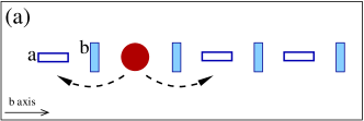
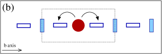
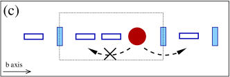
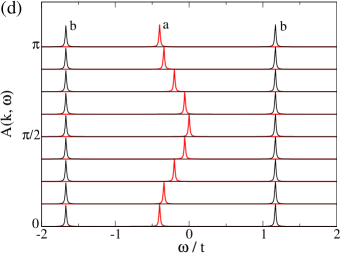
Figure 1: (Color online) Hole propagation in the 1D strong-coupling model (2). Two top panels show a hole doped into: (a) mobile $a$ orbitals (empty boxes), and (b) immobile $b$ orbitals (filled boxes). Solid (dashed) arrows indicate possible hopping processes with hopping elements $t$ and $\tau$, respectively; in case of a hole added to the $b$ orbital the latter process occurs only after the initial hopping by $t$, see panel (c). Panel (d) shows the exact spectral functions $A_{a}(k,\omega)$ and $A_{b}(k,\omega)$ of a hole added into the $a$ orbital (middle dispersive feature between $\omega=-0.4t$ and $\omega=0$) and the $b$ orbital (two side dispersionless maxima) as obtained from the 1D strong-coupling model (2). Parameters: $J=0.4t$, $\tau=0.1t$, and peak broadening $\delta=0.01t$. The spectral functions obtained using the VCA for the 1D Hubbard model (1) with $U=10t$ (not shown) are identical to the exact result.

When one attempts to calculate the Green’s function for a hole doped in the immobile $b$ orbital,

$$G_{b}(k,\omega)=\lim_{\delta\to 0}\,\left\langle 0\left|\,b_{k}^{\dagger}\frac{1}{\omega+{\cal H}_{\rm 1D}-E_{0}+i\delta}\,b_{k}\right|0\right\rangle\,,$$ (13)

one finds immediately that the state

$$|\psi_{k}^{(1)}\rangle\equiv b_{k}|0\rangle=\sqrt{\frac{2}{N}}\sum_{j\in B}e^{-ikR_{j}}b_{j}|0\rangle\,,$$ (14)

is not an eigenstate of the Hamiltonian ${\cal H}_{\rm 1D}$. Here a hole is doped in each Fourier component in an occupied $b$ orbital at site $j$ in the ground state with AO order (8). When a hole is doped it can delocalize to its neighbors in the 1D chain, as depicted in Fig. 1(b), so one has to introduce appropriate basis of states obtained when the single hole delocalizes along the 1D chain. The hopping $H_{t}$ acting on $|\psi_{k}^{(1)}\rangle$ generates the first (normalized) state

$$|\psi_{k}^{(2)}\rangle\equiv\frac{1}{\sqrt{N}}\sum_{j\in B}e^{-ikR_{j}}(a_{j-1}+a_{j+1})a_{j}^{\dagger}b_{j}|0\rangle\,,$$ (15)

with the hole delocalized to the neighboring $j-1$ ($j+1$) sites of the $A$ sublattice, i.e., to the the left (right) from the initial hole position $j$ in each Fourier component $|b_{j}\rangle$ included in Eq. (14). The remaining states $\{|\psi_{k}^{(n)}\rangle\}$ with $n>2$, which occur in the continued fraction expansion needed to evaluate the Green’s function $G_{b}(k,\omega)$ (see below), are generated by acting $(n-2)$ times on $|\psi_{k}^{(2)}\rangle$ with the three-site hopping term $H_{\rm 3s}$. In this way one finds the set of symmetric states, with a superposition of the hole propagating forward (either to the left or to the right from the initial defect), i.e., along the same direction as that given by the first hop which led to $|\psi_{k}^{(2)}\rangle$, cf. Fig. 1(c). This structure of the basis set explains the absence of the $k$ dependence in the Green’s function for $b$ orbitals, so we adopt the simplified notation $G_{b}(\omega)$ below.

In the infinite basis generated by the above described procedure, the Hamiltonian matrix of the Hamiltonian (2) reads:

$$\langle\psi_{k}^{(m)}|\,\omega+{\cal H}_{\rm 1D}-E_{0}|\psi_{k}^{(n)}\rangle=$$

$$=\left(\begin{array}[]{ccccc}\omega+J/2&\sqrt{2}t&0&0&...\\ \sqrt{2}t&\omega+3J/4&\tau&0&...\\ 0&\tau&\omega+J&\tau&...\\ 0&0&\tau&\omega+J&...\\ ...&...&...&...&...\\ \end{array}\right).$$ (21)

In order to calculate the relevant Green’s function $G_{b}(\omega)$, we need the $(1,1)$ element of the inverse of this matrix. Due to the tridiagonal form of the Hamiltonian, this can be done even for an infinite Hilbert space, and we arrive at a continued fraction result:

$$G_{b}(\omega) =\left\{\left\langle\psi_{k}^{(m)}\left|\omega+{\cal H}_{\rm 1D}-E_{0}\right|\psi_{k}^{(n)}\right\rangle^{-1}\right\}_{1,1}$$

$$=\left\{\omega+\frac{1}{2}J-\frac{2t^{2}}{\omega+\frac{3}{4}J-\frac{\tau^{2}}{\omega+J-\frac{\tau^{2}}{\omega+J-\dots}}}\right\}^{-1},$$ (22)

where the whole self-similar part can be summed up to the self-energy which does not depend on $k$:Bri70

$$\Sigma(\omega)\equiv\frac{\tau^{2}}{\omega+J-\frac{\tau^{2}}{\omega+J-\frac{\tau^{2}}{\omega+J-...}}}=\frac{\tau^{2}}{\omega+J-\Sigma(\omega)}.$$ (23)

This, together with Eq. (II.2), leads to a quadratic equation for $\Sigma(\omega)$ with two solutions:

$$\Sigma(\omega)=\frac{1}{2}\left\{(\omega+J)\pm\sqrt{(\omega+J)^{2}-4\tau^{2}}\,\right\}.$$ (24)

The proper sign may be determined using the Green’s function $G_{b}(\omega)$ obtained beforeDag04 in the limit of $\tau=0$,

$$G_{b}^{(0)}(\omega)=\left\{\omega+\frac{1}{2}J-\frac{2t^{2}}{\omega+\frac{3}{4}J}\right\}^{-1}\,.$$ (25)

In this limit the self-energy vanishes, $\Sigma(\omega)=0$, and the Green’s function has two poles at energies

$$\omega=-\frac{5}{8}J\pm\sqrt{2}t\,\sqrt{1+\frac{1}{128}\left(\frac{J}{t}\right)^{2}}.$$ (26)

Finally, we arrive at the general result for $\tau>0$:

$$G_{b}(\omega)=\left\{\omega+\frac{1}{2}J-\frac{4t^{2}}{\omega+\frac{1}{2}J\mp\sqrt{(\omega+J)^{2}-4\tau^{2}}}\right\}^{-1},$$ (27)

where the sign convention is fixed by comparing this result with the Green’s function $G_{b}^{(0)}(\omega)$ (25): This implies that one has to select $-$ ($+$) sign for $\omega<-J$ ($\omega>-J$), respectively.

Due to the obtained analytic structure of $G_{b}(\omega)$ the hole spectral function

$$A_{b}(\omega)=-\frac{1}{\pi}\,\mbox{Im}\,G_{b}(\omega),$$ (28)

shown in Fig. 1(d), also does not depend on $k$. For the realistic parameters with $\tau<t$ it consists of two poles and the incoherent part centered around $\omega=-J$. This latter contribution has rather low intensity and is thus invisible on the scale of Fig. 1(d), and the two peaks absorb almost the entire intensity. This result resembles the case of $\tau=0$ (26), and might appear somewhat unexpected – we analyze it in the following Section.

II.3 Hole confinement in a three-site box

First, we comment on the absence of the $k$ dependence in the spectral function $A_{b}(\omega)$ (28). It suffices to analyze the hole in a $b$ orbital at any finite value of $J$ which induces the AO ground state (8). The hole can only move incoherently, because once it moves away from the initial site $j$ [see Fig. 1(b) and (c)], it creates a defect in the AO state which blocks its hopping by the three-site processes over the site $j$, see Eq. (14). Consequently, the hole may hop only in the other direction, i.e. away from the defect in the AO state, and in order to absorb eventually this orbital excitation it has to come back to its original position, retracing its path. In this way a forward and backward propagation along the 1D chain interfere with each other, resulting in the fully incoherent spectrum of Fig. 1(d).

Looking at the spectral function $A_{b}(\omega)$ of a hole doped into the $b$ orbital at finite $\tau=0.1t$ shown in Fig. 1(d), one may be somewhat surprised that the result indicates only two final states of the 1D chain. These are the bonding and the antibonding state of a hole confined within a three-site box, and discussed in detail in Ref. Dag04, in the limit of $\tau=0$. One finds that the two excitation energies obtained for the present parameters, $\omega=-1.67t$ and $\omega=1.17t$, are indeed almost unchanged from those given by Eq. (26) at $\tau=0$. We note that the third nonbonding state has a different symmetry and thus gives no contribution to $A_{b}(\omega)$.

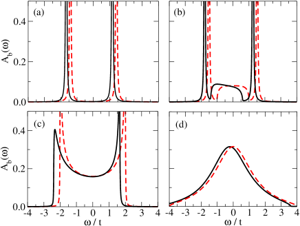
Figure 2: (Color online) Spectral function $A_{b}(\omega)$ of a hole doped into the $b$ orbital in the 1D model with: (a) $\tau=0$, (b) $\tau=0.5t$, (c) $\tau=t$, and (d) $\tau=2t$. Dotted (solid) lines for $J=0$ ($J=0.4t$), respectively, with broadening $\delta=0.01t$.

Altogether, one finds that in the realistic regime of parameters with $\tau=J/4$, the incoherent part of the spectrum is extremely small and thus invisible in the scale of Fig. 1(d). This implies that the hole is still practically trapped within the three-site box depicted on Fig. 1(b), in spite of the potential possibility of its delocalization by finite $\tau$. Only when the value of the three-site hopping $\tau$ is considerably increased, the hole can escape from the three-site box, and may delocalize over the entire chain.

A systematic evolution of the spectral function $A_{b}(\omega)$ with increasing $\tau$ is depicted in Fig. 2. One observes that the incoherent spectral weight grows with increasing $\tau$ and is already visible in between the two maxima for $\tau=0.5t$. When the three-site hopping term approaches $\tau=t$, the spectrum changes in a qualitative way — both peaks are absorbed by the continuum, and the spectral density resembles the density of states of the 1D chain with the NN hopping. For the extremely large effective hopping $\tau\simeq 2t$ the two peaks corresponding to the energies given by Eq. (26) are entirely gone, and the spectrum corresponds to the incoherent delocalization of the hole over the 1D chain. Note also that finite $J$ results only in an overall shift of the spectra due to the energy cost of the hole excitation in the ordered ground state (8).

III 2D spinless Falicov-Kimball model

III.1 Effective strong-coupling model

There are two essentially different ways to generalize the 1D orbital Hubbard model with one passive orbital flavor to two dimensions in such a way that the superexchange remains still Ising-like. Either (i) one allows that the electrons with mobile flavor $a$ can hop along all the bonds, i.e. in both directions in the square lattice, or (ii) one allows that $a$ electrons can hop along the bonds parallel to the $b$ axis, and $b$ electrons can hop along the bonds parallel to the $a$ axis. The first scenario leads to a special case of the 2D FK model (see below), while the second one describes spinless electrons in $t_{2g}$ orbitals of a FM plane and will be analyzed in Sec. V.

In analogy to the 1D model of Sec. II, the 2D FK model describes interacting electrons in mobile $a$ and immobile $b$ orbitals,

$$H_{\rm FK}=-t\sum_{\langle ij\rangle}(a^{\dagger}_{i}a_{j}+\mbox{h.c.})+U\sum_{i}n_{ia}n_{ib}\;.$$ (29)

Here we used the same notation as in Eq. (1), and $\langle ij\rangle$ are the bonds (pairs of NN sites) in the 2D lattice. This Hamiltonian shows complex physicsBry08 and phase separationMas06 away from half filling. In contrast to the usual situation with large energy difference between $f$ and $d$ orbitals,Fre03 we will consider degenerate $a$ and $b$ orbitals. Then the ground state at half filling (i.e., one electron per site) and large Coulomb interaction $U$ is relatively straightforward to investigate, and one finds the robust AO order rather then phase separation.

Again, we can perform second order perturbation theory in the regime of $t\ll U$ as above. For the present square lattice there are two types of three-site terms — they contribute: (i) along $a$ and $b$ axes due to forward (linear) processes, and also (ii) connect next-nearest neighbor (NNN) sites along the diagonals of each plaquette in the 2D lattice, along two $90^{\circ}$ paths. The resulting strong-coupling effective Hamiltonian reads

$${\cal H}_{\rm FK}=H_{t}+H_{J}+H_{\rm 3s}^{(l)}+H_{\rm 3s}^{(d)},$$ (30)

where

$$H_{t} = -t\sum_{\langle ij\rangle}(\tilde{a}^{\dagger}_{i}\tilde{a}_{j}+\mbox{h.c.}),$$ (31)

$$H_{J} = \frac{1}{2}J\sum_{\langle ij\rangle}\left(T^{z}_{i}T^{z}_{j}-\frac{1}{4}\tilde{n}_{i}\tilde{n}_{j}\right)\,,$$ (32)

$$H_{\rm 3s}^{(l)} = -\tau\sum_{i}\left(\tilde{a}^{\dagger}_{i-\bf{\hat{a}}}\tilde{n}_{ib}\tilde{a}_{i+\bf{\hat{a}}}\!+\!\mbox{h.c.}\right)$$ (33)

$$-\tau\sum_{i}\left(\tilde{a}^{\dagger}_{i-\bf{\hat{b}}}\tilde{n}_{ib}\tilde{a}_{i+\bf{\hat{b}}}+\!\mbox{h.c.}\right)\!,$$

$$H_{\rm 3s}^{(d)} = -\tau\sum_{i}\left(\tilde{a}^{\dagger}_{i\pm\bf{\hat{b}}}\tilde{n}_{ib}\tilde{a}_{i\pm\bf{\hat{a}}}\!+\!\mbox{h.c.}\right)$$ (34)

$$-\tau\sum_{i}\left(\tilde{a}^{\dagger}_{i\mp\bf{\hat{b}}}\tilde{n}_{ib}\tilde{a}_{i\pm\bf{\hat{a}}}\!+\!\mbox{h.c.}\right)\!\!.$$

Here $\bf{\hat{a}}$ and $\bf{\hat{b}}$ are the unit vectors along the axes $a$ and $b$, while $H_{\rm 3s}^{(l)}$ and $H_{\rm 3s}^{(d)}$ terms stand for linear and diagonal processes in the three-site effective hopping. The parameters $J$ and $\tau$ are defined as in Eqs. (7), the orbital (pseudospin) operators $T^{z}_{i}$ are defined as in Eq. (6), and again the tilde above the fermion operators indicates that the Hilbert space is restricted to the unoccupied and singly occupied sites.

III.2 Analytic Green’s functions

The Green’s function $G_{a}({\bf k},\omega)$ for a hole in mobile $a$ orbitals, defined by Eq. (9), can be calculated as straightforwardly as in the 1D model of Sec. II, and one finds:

$$G_{a}({\bf k},\omega)=\frac{1}{\omega+J+\varepsilon_{\bf k}}\;,$$ (35)

where the hole dispersion relation is given by

$$\begin{split}\varepsilon_{\bf k}=-4\tau\left\{(\cos k_{x}+\cos k_{y})^{2}-1\right\}\,.\end{split}$$ (36)

As in the 1D model, see Eq. (11), the hole propagates freely, resulting in a bandwidth of $W=16\tau=4J$. Indeed, in the strong-coupling model (30) the hopping to the sites occupied by $b$ electrons is blocked by the constraint. The spectral function $A_{a}({\bf k},\omega)$ (12) obtained for the hole in $a$ orbitals consists thus of a single pole, as shown in Fig. 3(a).

The dispersion relation of Eq. (36) can be compared with the one of the lower Hubbard band obtainedMas06 for the FK model (29) in the regime of $U\gg t$, where one finds dispersion

$$\epsilon_{\bf k} = \frac{1}{2}U\left\{1-\sqrt{1+\frac{16t^{2}}{U^{2}}(\cos k_{x}+\cos k_{y})^{2}}\right\}$$ (37)

$$\simeq -4\tau(\cos k_{x}+\cos k_{y})^{2}\,.$$

This result is the same (up to a nonsignificant constant) as the one obtained in the strong-coupling limit, see Eq. (36). The Green’s function obtained for the Hubbard-like model (29) is shown in Fig. 3(b). While it qualitatively agrees with the result derived in the strong-coupling limit (36), it is here renormalized and gives a somewhat reduced bandwidth of the hole band. This indicates finite probability of double occupancies which hinder the three-site effective hopping processes, and reduce the order parameter from its classical value as given in the Néel state (8), see also Sec. V.5 for a similar discussion concerning the 2D $t_{2g}$ orbital model.

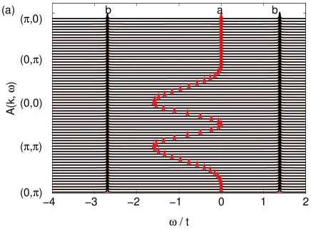
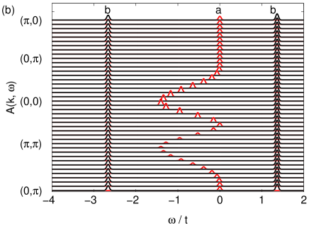
Figure 3: (Color online) The spectral functions for the 2D FK model, as obtained for mobile $a$ orbitals (middle dispersive feature between $\omega=-1.6$ and $\omega=0$) and immobile $b$ orbitals (two side dispersionless maxima): (a) with the RPA of Ref. Bri70, for the 2D FK strong-coupling model (30) with $J=0.4t$ and $\tau=0.1t$, and (b) by a numerical diagonalization of a $20\times 20$ cluster for the 2D FK Hubbard model (29) with $U=10t$. Peak broadening $\delta=0.01t$.

As in the 1D model of Sec. II.2, we use here the RPA to calculate the Green’s function for a hole inserted into the immobile $b$ orbital. However, the RPA is no longer exact in two dimensions, because also paths with closed loops are possible when electrons with one flavor are allowed to hop in both directions. We use a similar basis of states $\{|\psi_{\bf k}^{(n)}\rangle\}$ as for the 1D calculation of Sec. II.2 to describe a single hole doped to the plane with the AO order. Starting from the Néel state as in Eq. (8), the first two states are defined as follows:

$$|\psi_{\bf k}^{(1)}\rangle\!\! \equiv \!b_{\bf k}|0\rangle=\sqrt{\frac{2}{N}}\sum_{j\in B}e^{-i{\bf k}{\bf R}_{j}}b_{j}|0\rangle\,,$$ (38)

$$|\psi_{\bf k}^{(2)}\rangle\!\! \equiv \!\frac{1}{\sqrt{2N}}\sum_{j\in B}e^{-i{\bf k}{\bf R}_{j}}$$ (39)

$$\times \!\!\left(a_{j-\bf{\hat{a}}}+a_{j+\bf{\hat{a}}}+a_{j-\bf{\hat{b}}}+a_{j+\bf{\hat{b}}}\right)a_{j}^{\dagger}b_{j}|0\rangle\,.$$

Here the first state $|\psi_{\bf k}^{(1)}\rangle$ denotes the Fourier transformed states with hole doped into the immobile orbital at the initial position in the ground state of the 2D lattice, with AO order between two sublattices $A$ and $B$, as in (8), see Fig. 4(a). This state may delocalize by the hopping $t$ which interchanges the hole with an occupied $a$ orbital to the left, right, down, or up from the initial site, resulting in the symmetric state with four external sites of the five-site polaron depicted in Fig. 4(b) — the resulting state is denoted above by $|\psi_{\bf k}^{(2)}\rangle$ (39).

At this point, we have to introduce an approximation and we will consider only these states $|\psi_{\bf k}^{(n)}\rangle$ with $n>2$ which are created on a Bethe lattice by 9 possible forward going steps from $|\psi_{\bf k}^{(n-1)}\rangle$. Therefore, all such states (with $n>2$) are generated by the three-site effective hopping $\tau$, so each of them means that the hole has moved forward by $(n-2)$ steps from the symmetric state $|\psi_{\bf k}^{(2)}\rangle$, being a linear combination of the configurations with the hole at one of the external sites in the five-site polaron (Fig. 4). Hence, we make two approximations here, i.e., we assume that: (i) no closed loops occur (RPA), and (ii) the number of forward going steps is chosen to be $9$ which is the most probable number of possible forward-going three-site steps on a square lattice with the AO order.notebet Let us emphasize, however, that the closed loops which are neglected here do not lead to the delocalization of the hole as these are not the so-called Trugman loopsTru88 where the hole could repair the defects by a circular motion around a plaquette in the square lattice. The Hamiltonian [Eq. (30)] matrix written in this basis is as follows:

$$\langle\psi_{\bf k}^{(m)}|\,\omega+{\cal H}_{\rm FK}-E_{0}|\psi_{\bf k}^{(n)}\rangle=$$

$$=\left(\begin{array}[]{ccccc}\omega+J&2t&0&0&...\\ 2t&\omega+\frac{7}{4}J+2\tau&3\tau&0&...\\ 0&3\tau&\omega+2J&3\tau&...\\ 0&0&3\tau&\omega+2J&...\\ ...&...&...&...&...\\ \end{array}\right).$$ (45)

Again, as in Eq. (II.2), the ${\bf k}$-dependence is absent, and the Green’s function $G_{b}(\omega)$ can be calculated using continued fraction method in a similar way as in the 1D case (cf. Sec. II.2) and we obtain

$$G_{b}(\omega)\!\! = \!\!\left\{\omega+J\right.$$ (46)

$$- \!\!\left.\frac{8t^{2}}{\omega+\frac{3}{2}J+4\tau\mp\sqrt{(\omega+2J)^{2}-36\tau^{2}}}\right\}^{-1}\!\!,$$

where we select $-$ $(+)$ sign for $\omega<-2J$ $(\omega>-2J)$, respectively.

\psfrag{A}{}\psfrag{B}{}\psfrag{t}{$t$}\psfrag{J4}{$\tau$}\includegraphics[width=99.73074pt]{holot4a.eps}

\psfrag{A}{}\psfrag{B}{}\psfrag{t}{$t$}\psfrag{J4}{$\tau$}\includegraphics[width=99.73074pt]{holot4b}

Figure 4: (Color online) Schematic view of a five-site polaron which occurs after the removal of one $b$-electron in the 2D FK model (30). (a) Initial state with a hole (empty circle) on $B$ sublattice — crosses represent immobile $b$ electrons and filled circles mobile $a$ electrons. Five-site polaron is indicated by the dotted line. (b) The hole may delocalize within it to the nearest neighbors by hopping $t$ (solid line), generating three broken bonds which cost energy $3J/4$ for each hopping process. The hole can hop directly between the external sites (dashed line) by second order three-site hopping $\tau=J/4$ via a doubly occupied site (outside the polaron).

The spectral function of a hole doped into the $b$ orbital is shown in Fig. 3(a). It consists of two distinct dispersionless peaks, and a dispersionless incoherent part with negligible spectral weight [invisible on the scale of Fig. 3(a)] between them. While the incoherent spectrum disappears in the limit of vanishing three-site hopping $\tau$, the two dispersionless peaks survive and the distance between them becomes $4t$ for $J\to 0$. Hence, the doped hole is not only immobile but also trapped within the five-site orbital polaron depicted in Fig. 4 – only four sites can be reached from the central site by NN hopping $t$, so the ground state can be found in the truncated basis $\{|\psi_{\bf k}^{(1)}\rangle,|\psi_{\bf k}^{(2)}\rangle\}$ (see below). This situation resembles very much the 1D case discussed previously, and indeed the same discussion as the one for the hole confinement in a three-site box presented in Sec. II.3 applies here. In the next Section we discuss in detail the quantitative arguments which suggest the hole confinement in this five-site polaron.

We would like to emphasize that the spectral functions obtained using the RPA for the strong-coupling model Eq. (30) are almost identical to the ones obtained numerically by exact diagonalization of the Hubbard model (29) on a $20\times 20$ lattice, cf. Fig. 3(b). This means that the crude assumption of walks without closed loops made within the RPA approximation (i.e., replacement of the square lattice by the Bethe lattice) is a posteriori well justified for the strong-coupling model defined by Eq. (30). We provide also more arguments which complete our understanding of this result in the next Section. Furthermore, this means that not only the RPA method is correct but also the two models (Hubbard and the strong-coupling model) are fully equivalent and describe the same physics in the considered regime of parameters.

Finally, we note that the results obtained by the VCA (not shown) are very similar to the ones of exact diagonalization, if we use periodic boundary conditions. While open boundaries are usually optimal for the VCA,Aic03 they can ‘cut’ the five-site polaron and lead to signals at wrong frequencies. In a large enough cluster, these contributions from polarons with less than five sites would have vanishing weight, but for the cluster sizes considered here, self-energies with periodic boundary conditions have to be used to eliminate them.

III.3 Localized five-site orbital polaron

The following comparison shows that the two dominant peaks of the Green’s function for $b$ orbitals $G_{b}(\omega)$ can be well reproduced by taking into account the polaron alone, i.e., by considering just a cluster of five sites depicted in Fig. 4 and neglecting the rest of the lattice. In this case the problem can be solved by diagonalizing the Hamiltonian in the basis consisting of two states defined in the last section: $|\psi_{\bf k}^{(1)}\rangle$ (38) and $|\psi_{\bf k}^{(2)}\rangle$ (39). This means that the infinite matrix of Eq. (III.2) for the hole doped into the central site of the polaron reduces to the $2\times 2$ matrix and one obtains the energies of two poles of the Green’s function $G_{b}(\omega)$, corresponding to the bonding and antibonding state within the five-site polaron:

$$\omega_{1,2}=-\frac{11}{8}J-\tau\pm\sqrt{4t^{2}+\frac{9}{64}J^{2}+\frac{3}{4}J\tau+\tau^{2}}\,.$$ (47)

Assuming $J=0.4t$ and $\tau=0.1t$ in Eq. (47) we obtain $\omega_{1,2}=\{1.37t,-2.67t\}$. This compares very favorably with the results obtained for the strong-coupling model (30): (i) within the RPA (see Sec. III.2), $\omega_{1,2}=\{1.38t,-2.69t\}$, and (ii) using the numerical analysis of this model on the $20\times 20$ lattice, which gives $\omega_{1,2}=\{1.40t,-2.74t\}$ (not shown). We stress that the excellent agreement between all these methods demonstrates that the RPA (i.e., full continued fraction) turns out to be only slightly better than the calculation restricted to the five-site polaron of Fig. 4. It means that the probability of the configurations with the hole outside the five-site polaron is indeed very low, and it explains why the RPA assumption of having no walks with closed loops works here so well. Lastly, we note that all these results agree quite well with the numerical ones for the itinerant FK model (29), cf. Fig. 3(b) with the peaks situated at $\omega_{1}=1.42t$ and $\omega_{2}=-2.56t$.

The present five-site orbital polaron resembles the five-site spin polaron identified in Monte Carlo studies for the 2D Kondo model. Dag04a For example, as for the spin polaron in the Kondo model, the spectral density of the orbital polaron is comprised of two dispersionless peaks with a distance of $4t$ for $J\to 0$. There is, however, one difference: Here not only the hole can move by direct NN hopping $t$ between the central site and the four external sites, but there is also a second order three-site diagonal hopping (34) which couples directly the neighboring external sites of the polaron (see Fig. 4), and contributes to the energy of the $|\psi_{\bf k}^{(2)}\rangle$ state. Actually, due to the inclusion of these processes (which enable the smallest loops on the lattice, with two $t$ and one $\tau$ hopping processes) we could obtain the above mentioned perfect agreement between the numerical, the RPA, and the five-site polaron results for the strong-coupling version of the FK model Eq. (30). Otherwise, e.g. for $J=0.4t$ the energies of the two peaks in the RPA (five-site polaron) calculation would be equal to $\{1.47t,-2.58t\}$ [$\{1.46t,-2.56t\}$], respectively, and would only rather poorly agree with the numerical results of Eq. (30).

Summarizing, the holes doped into the immobile orbitals of the FK model are almost entirely localized within the five-site orbital polaron of Fig. 4. In order to calculate the energy of this polaron correctly one has to take into account the energies of the processes which involve four external polaron sites. In addition, we note that the widely used SCBAMar91 (used for the orbital strong-coupling model in the next Section) does not work so well for the case of hole doped into the immobile orbital of the FK model, as it does not respect the constraint on the hole motion. It incorrectly uses an on-site energy of $J$ instead of $3J/4$ for the excitations at external sites of the polaron. As shown above, the hole spends almost all its time inside the polaron and hence this underestimation of the energy heavily influences the energies of the poles of the Green’s function in this case [e.g. the lowest peak for $J=0.4t$ is situated almost at $-3t$ in the SCBA calculations (not shown)].

IV string excitations in the 1D model

The 1D model (Sec. II) and the 2D FK model (Sec. III) bear the same generic features: (i) a hole generated in the so-called mobile orbital always leads to the dispersive spectrum with the full unrenormalized bandwidth, and (ii) a hole doped into the so-called immobile orbital is localized, leading to a non-dispersive spectral function. In this Section we investigate the consequences of string excitations which may arise when both orbital states allow only 1D hopping, as in the case of two $t_{2g}$ orbitals lying in two vertical planes with respect to the considered plane. Thus we will study the 1D model with electrons hopping between $yz$ and $zx$ orbitals in $(a,b)$ plane — the model has only $2N$ sites for the chain of length $N$, see Fig. 5. We will show that even the shortest possible strings with the length of one bond which can be excited here when the hole moves in this geometry are sufficient to generate some characteristic features recognized later in the spectral properties of the 2D $t_{2g}$ model (see Sec. V).

The 1D model of Fig. 5(a) consists of a chain along $b$ axis, with the Hamiltonian as described by Eq. (1), and two sites being the NNs of every second site of the chain along the $a$ axis, which could represent radicals added to a linear molecule. We use here the convention introduced before for the $t_{2g}$ orbital systems,Kha01 ; Ole05 that $a$ and $b$ orbitals stand for $yz$ and $zx$ $t_{2g}$ orbitals, respectively, that permit the electron hopping along the $b$ and $a$ axis in the $(a,b)$ plane. The Hamiltonian of the present (called here centipede) model is,

$$H_{\rm c} = -t\sum_{i}\left\{b^{\dagger}_{2i}(b_{2i,u}+b_{2i,d})+\textrm{h.c.}\right\}$$ (48)

$$- t\sum_{i}(a^{\dagger}_{i}a_{i+1}+\textrm{h.c.})+U\sum_{i}n_{ia}n_{ib}\;.$$

The hopping along the bonds parallel to the $a$ axis is allowed only to the orbitals $b$, with the corresponding creation operators $\{b^{{\dagger}}_{2i,u},b^{{\dagger}}_{2i,d}\}$, see Fig. 5(a). To simplify notation, we call these orbitals $u$ and $d$, and introduce the following operators:

$$u^{{\dagger}}_{2i}\equiv b^{{\dagger}}_{2i,u},\hskip 28.45274ptd^{{\dagger}}_{2i}\equiv b^{{\dagger}}_{2i,d}\;.$$ (49)

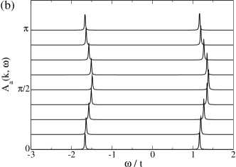
Figure 5: (Color online) Propagation of a hole added into the $a$ orbital in the centipede strong-coupling model (50): (a) schematic picture of a hole doped at site $a$ and its possible delocalization via hopping $t$ (solid lines) and three-site effective $\tau$ term (dashed lines); (b) spectral function $A_{a}(k,\omega)$. Parameters: $J=0.4t$, $\tau=0.1t$, peak broadening $\delta=0.01t$. The chain is oriented along the $b$ axis, and nonequivalent positions of the orbitals which do not permit hopping along this direction are labelled $b$, $u$ and $d$ in panel (a).

In the limit of large $U$ ($U\gg t$) the occupied orbitals form AO order along the chain and we select the Néel state with $b$ ($u$ and $d$) orbitals occupied on the external sites, as shown in Fig. 5, as we are interested in their effect on the hole propagation when it was doped to an $a$ orbital. This leads to the following strong-coupling version of the 1D centipede model (48):

$${\cal H}_{\rm c}\! = -t\,\sum_{i}\{(\tilde{u}^{\dagger}_{2i}+\tilde{d}^{\dagger}_{2i})\tilde{b}_{2i}+\textrm{h.c.}\}$$ (50)

$$- \tau\sum_{i}(\tilde{a}^{\dagger}_{2i}\tilde{n}_{2i+1,b}\tilde{a}_{2i+2}+\textrm{h.c.})$$

$$- \frac{3}{4}J\sum_{i}(\tilde{u}^{\dagger}_{2i}\tilde{u}_{2i}+\tilde{d}^{\dagger}_{2i}\tilde{d}_{2i})\,.$$

On the one hand, the superexchange interaction for all the bonds within the centipede was not included in Eq. (50) as it results only in a rather trivial energy shift of the spectra obtained from the Green’s function $G_{a}(k,\omega)$ which is of interest here,notenob cf. Sec. II.2. On the other hand, the last term in Eq. (50) was added to simulate the creation of string excitations which occur in the full 2D model of Sec. V (see also discussion below).

Whereas the second term in Eq. (50) is once again the three-site hopping derived before in the 1D model (5) [cf. Fig. 5(a)], the other two terms describe the possibility of creating defects in the AO order when the hole leaves the spine of the centipede (i.e., moves away from the $a$ sites) by creating strings of length one, just as it may happen in the $t_{2g}$ 2D model, see Sec. V. Here the hole can leave the chain to its NN orbital $u_{2i}$ or $d_{2i}$ [cf. sites attached to the chain along the $a$ axis shown in Fig. 5(a)]. Such defects are created by hopping $t$ and costs energy $3J/4$ in each case. Hence, the present 1D model represents an extreme reduction of the full $t_{2g}$ 2D model, allowing only the strings of length one, and each defect has to be deexcited before the hole can hop to another three-site unit along the chain. Note however, that the energies of these string excitations are properly chosen and are just the same as in the full 2D model of Sec. V.

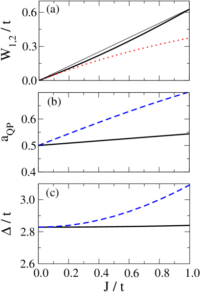
Figure 6: (Color online) Characteristic features in the spectra obtained for the 1D centipede model (Fig. 5) for increasing $J$: (a) the bandwidth $W_{1,2}$, (b) the spectral weight $a_{\rm QP}$, and (c) the distance $\Delta$ between the two peaks. The solid (dotted) line in (a) corresponds to the first (second) dispersive peak in $A_{a}(k,\omega)$ whereas the solid (dashed) lines in the lower panels show results for $k=0$ ($k=\pi/2$), respectively. The light solid line in (a) is merely a guideline for the eye to show that the bandwidth of the first peak is a function with a positive second derivative. Parameter: $\tau=J/4$.

The model given by Eq. (50) constitutes a one-particle problem (after inserting $\tilde{n}_{2i+1,b}\equiv 1$ which is consistent with the Ising nature of the superexchange) and hence can be solved exactly. We will consider the Green’s function $G_{a}(k,\omega)$ for $a$ orbitals, defined similarly as in Eq. (9), and a hole excitation is created again by the operator $a_{k}$ of Eq. (10). The continued fraction terminates after the second step and one finds the exact Green’s function

$$G_{a}(k,\omega)=\frac{1}{\omega+2\tau\cos(2k)-\frac{2t^{2}}{\omega+\frac{3}{4}J}}\,,$$ (51)

leading to the corresponding spectral function $A_{a}(k,\omega)$, defined as in Eq. (12). The numerical results obtained with $J=0.4t$ are shown in Fig. 5(b). Instead of a single dispersive state of Fig. 1(d), the spectral function consists here of two dispersive peaks, separated by a gap of roughly $2\sqrt{2}t$. This demonstrates that the larger hopping $t$ suppresses at first instance the hopping along the chain by the element $\tau$, and a hole doped into the $a$ orbital delocalizes in first place over the three-site unit, discussed in Sec. II.3, consisting of a hole and two $b$ ($u$ and $d$) orbitals. Therefore, the hole behaves effectively as a defect created at a $b$ site in the 1D chain of Sec. II. This explains that the maxima of $A_{a}(k,\omega)$ are found again for a bonding and antibonding state, similar to the structure of $A_{b}(\omega)$ in Sec. II.2. However, at present the corresponding states gain weak dispersion because the hole may as well delocalize along the chain by the three-site hopping $\tau$. Note also that the low-energy (right) peak has slightly higher dispersion (leading to a broader band) than the left one. This case illustrates that the 1D dispersion is broader for the QP state but is also shared by the feature at higher energy. This observation will help us to interpret the spectra for the 2D $t_{2g}$ model in Sec. V.

In addition we also calculated some characteristic features of the spectra of the centipede model, cf. Fig. 6. They will mostly serve for a comparison with the respective results of the 2D $t_{2g}$ model, presented in Sec. V.5. However, let us only remark that the renormalization of the bandwidth, shown in Fig. 6(a) follows from an intricate interplay between coherent hole propagation and the string excitations. With increasing $\tau=J/4$ the free bandwidth increases but at the same time the energies of the defects (generated by the hole when it moves to ’lower’ or ’upper’ sites) are $\propto J$; hence, the bandwidth does not depend in a linear way on $J$, cf. Fig. 6(a). Physically this means that the hole motion is gradually more and more confined to just the 1D path along the chain with increasing $J$ (and keeping $\tau=J/4$).

V 2D model for $t_{2g}$ electrons

V.1 Effective strong-coupling model

After analyzing the spectral properties of the simpler 1D model and 2D FK model, we consider below the model relevant for transition metal oxides with active $t_{2g}$ orbitals, when the crystal field splits them into $e_{g}$ and $a_{1}$ states, and the doublet $e_{g}$ is filled by one electron per site. This occurs for the $d^{1}$ configuration (e.g. in the titanates) when the $e_{g}$ doublet has lower energy than the $a_{1}$ state, or for $d^{2}$ configuration when the $e_{g}$ states have higher energy and are considered here, while the $a_{1}$ state is occupied by one electron at each site and thus inactive (as in the high-spin ground state of the $R$VO₃ perovskites,Hor03 where $R$ stands for a rare earth element). To be specific, we consider electrons with two $t_{2g}$ orbital flavors, $yz\equiv a$ and $zx\equiv b$, moving within the $(a,b)$ plane. In contrast to the FK model with two nonequivalent orbitals and only one orbital flavor contributing to the kinetic energy (Sec. III), both $t_{2g}$ orbitals are here equivalent and electrons can propagate conserving the orbital flavor by the NN hopping $t$, but only along one direction in the $(a,b)$ plane.Kha01 While this results is a complicated many-body problem at arbitrary electron filling, the motion of a single hole added at half filling remains still strictly 1D. Dag08

The orbital Hubbard model for spinless electrons in the FM $(a,b)$ plane reads:

$$H_{t_{2g}} = -t\sum_{\langle ij\rangle\parallel a}(b^{\dagger}_{i}b_{j}+\mbox{h.c.})-t\sum_{\langle ij\rangle\parallel b}(a^{\dagger}_{i}a_{j}+\mbox{h.c.})$$ (52)

$$+ U\sum_{i}n_{ia}n_{ib},$$

where $a$ and $b$ are the orbital flavors with the same hopping $t$ along $b$ and $a$ axis, respectively, and $U$ stands again for the on-site interaction energy for a doubly occupied configuration. At the filling of one electron in $\{a,b\}$ orbitals per site this interaction corresponds to the high-spin $d^{2}$ (or $d^{3}$) state. Second order perturbation theory applied to this Hamiltonian in the regime of $t\ll U$ leads then to the strong-coupling model,

$${\cal H}_{t_{2g}}=H_{t}+H_{J}+H_{\rm 3s}^{(l)}+H_{\rm 3s}^{(d)},$$ (53)

where

$$H_{t} = -t\sum_{i}(\tilde{b}^{\dagger}_{i}\tilde{b}_{i+\bf{\hat{a}}}+\tilde{a}^{\dagger}_{i}\tilde{a}_{i+\bf{\hat{b}}}+\mbox{h.c.})\,,$$ (54)

$$H_{J} = \frac{1}{2}J\sum_{\langle ij\rangle}\left(T^{z}_{i}T^{z}_{j}-\frac{1}{4}\tilde{n}_{i}\tilde{n}_{j}\right)\,,$$ (55)

$$H_{\rm 3s}^{(l)} = -\tau\sum_{i}(\tilde{b}^{\dagger}_{i-\bf{\hat{a}}}\tilde{n}_{ia}\tilde{b}_{i+\bf{\hat{a}}}+\mbox{h.c.})$$ (56)

$$-\tau\sum_{i}(\tilde{a}^{\dagger}_{i-\bf{\hat{b}}}\tilde{n}_{ib}\tilde{a}_{i+\bf{\hat{b}}}+\mbox{h.c.})\,,$$

$$H_{\rm 3s}^{(d)} = -\tau\sum_{i}(\tilde{a}^{\dagger}_{i\pm\bf{\hat{b}}}\tilde{a}_{i}\tilde{b}^{\dagger}_{i}\tilde{b}_{i\pm\bf{\hat{a}}}+\mbox{h.c.})$$ (57)

$$-\tau\sum_{i}(\tilde{a}^{\dagger}_{i\mp\bf{\hat{b}}}\tilde{a}_{i}\tilde{b}^{\dagger}_{i}\tilde{b}_{i\pm\bf{\hat{a}}}+\mbox{h.c.})\,.$$

The parameters $J$ and $\tau$ are defined as in Eqs. (7), whereas the pseudospin operators $T^{z}_{i}$ are defined as in Eq. (6). Again the tilde above the fermion operators indicates that the Hilbert space is restricted to the unoccupied and singly occupied sites. One interesting observation here is that the strictly 1D kinetic energy of the two orbitals leads to the 2D superexchange (55). As in the spin case,Cha77 the superexchange is active only when electrons with two different flavors occupy the neighboring sites (one bond), but here only one of them can hop, which explains the prefactor $\frac{1}{2}$ in Eq. (55).

Instead of the quantum behavior and frustration present in the compass model,Mos03 here one finds that the perfect AO ordered state $|0\rangle$ (8) is the ground state of the model at half filling. Figure 7 presents in a schematic way a few first steps in the motion of a hole inserted at a selected site into such a ground state. When the hole moves via NN hopping $t$, it creates string excitations in each step that cannot be healed by orbital flips, because the orbital superexchange (55) is purely Ising-like, see Fig. 7(c). Moreover, it cannot heal the defects by itself, because it cannot complete a Trugman loopTru88 when the orbital defects are created and three occupied orbitals are moved anticlockwise on a plaquette after the hole moved clockwise by three steps, see Fig. 7(d).

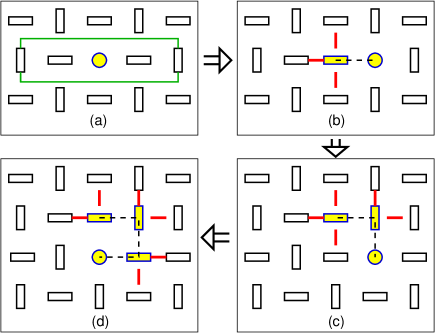
Figure 7: (Color online) Schematic view of the hole motion in the strong coupling $t_{2g}$ orbital model (52) with AO order. Circles depict holes while horizontal (vertical) rectangles depict occupied orbitals with electrons that can move only horizontally (vertically), respectively. The hole inserted in the AO state (a) can move via NN hopping $t$, but it has to turn by 90^∘ in each step along its path and leaves behind broken bonds leading to string excitations with ever increasing energy (b) and (c). After moving by 270^∘ around a plaquette (d), the hole cannot return to its initial position as would be necessary to complete the Trugman path. Tru88

The structure of ${\cal H}_{t_{2g}}$ (53) is similar to that of the 2D FK model — one obtains again three-site terms in the strong-coupling model along the axes (to third neighbors) (56) as well as along the plaquette diagonals (to second neighbors) (57). However, there is now an important difference to the 2D FK model: While three-site terms along the axes, given in Eq. (56), involve a single electron and conserve orbital flavor, terms along the diagonal (57) require the subsequent hopping of two electrons with different orbital flavor in each step, so the orbital flavor (at the site where the double occupancy is created in the excited state) is flipped. We will see later that such terms flipping orbital flavor are in fact suppressed, because, in contrast to the forward hopping along one of the cubic axes, they disturb the AO order in the background and thus cost energy. As such, they do not affect the low-energy QP state, but contribute only to the incoherent processes at higher energy.

To achieve a complete understanding of the excitation spectra at half filling, we used two complementary methods and investigated the orbital Hubbard model (52) using the VCA, and the strong-coupling model (53) within the SCBA. Both cases were supplemented by exact diagonalization for small ($4\times 4$ and $4\times 6$ sites) clusters. In the following Section we formulate the SCBA treatment of the $t_{2g}$ model, next give results of the SCBA calculations in Sec. V.3, compare them to a numerical VCA treatment in Sec. V.4, and discuss the QP properties in Sec. V.5. Finally, the impact of longer-range hopping pertinent to realistic materials is treated in Sec. VI.

V.2 Hole-orbiton coupling in the $t_{2g}$ model

The calculation of spectral properties of the strong-coupling model given by Eq. (53) is more involved than in the previous cases. On the one hand, in each such step by hopping $t$ the position of a hole is interchanged with an electron and a defect in the AO state is created (see Fig. 7). Therefore, one arrives at a situation analogous to a hole which tries to propagate in an antiferromagnet with the Ising interactions.Kan89 On the other hand, the important new feature which makes the present $t_{2g}$ problem more complex is that the electron hopping $t$ is now allowed for both orbital flavors. Thus, this problem cannot be solved by the RPA noteis , which was used to determine the Green’s functions $G_{a}(\bf{k},\omega)$ and $G_{b}(\bf{k},\omega)$ of a hole doped into the $a$ and $b$ orbital in either the 1D models or in the 2D FK model. Moreover, this problem cannot be reduced to any effective one-particle Hamiltonian that one could solve at least numerically for large clusters. Hence, we use below the SCBA which gives quite reliable results in the spin case.Mar91 Here one finds that it is well designed to treat this problem because several processes not included in the SCBA drop out of the Hamiltonian (53) for physical reasons (see below), and therefore the approximation performs remarkably well.

In order to implement the SCBA we have to reduce the model of Eq. (53) into the polaron problem, following Ref. Mar91, . Firstly, we divide the square lattice into two sublattices $A$ and $B$, such that all the $a$ ($b$) orbitals are occupied in the perfect AO state in sublattice $A$ ($B$), respectively, see Eq. (8). Secondly, we rotate the orbital pseudospins on the $A$ sublattice [corresponding the down orbital flavor, see Eq. (6)] so that all the pseudospin operators take a positive value, $\langle T^{z}_{i}\rangle=1/2$, in the transformed ground state. Finally, we introduce boson operators $\alpha_{i}$ (responsible for orbital excitations – orbitonsvdB99 ) and fermion operators $h_{i}$ (holons), which are related to the ones in the original Hilbert space by the following transformation:

$$\tilde{b}_{i}\equiv h_{i}^{\dagger}(1-\alpha_{i}^{\dagger}\alpha_{i}),\hskip 19.91684pt\tilde{a}_{i}\equiv h_{i}^{\dagger}\alpha_{i}.$$ (58)

Note, that we added the projection operators $(1-\alpha_{i}^{\dagger}\alpha_{i})$ to the transformation relation for the $\tilde{b}_{i}$ fermions in order to keep track of the violation of the local constraint that ’no hole and orbiton can be present at the same site’, cf. constraint $C1$ in Ref. Mar91, .

Before writing down the polaronic Hamiltonian, we make the following approximations: (i) keep only linear terms in boson operators (as we use linear orbital-wave approximationvdB99 ), (ii) skip $(1-h_{i}^{\dagger}h_{i})$ and $(1-\alpha_{i}^{\dagger}\alpha_{i})$ projection operators when deriving the effective Hamiltonian (both simplifications are allowed for the present case of one hole and Ising superexchange), and (iii) neglect the orbital-flipping terms Eq. (57) as generating the coupling between the hole and two orbitons and leading to higher-order processes in the perturbation theory. Then, after Fourier transformation, the Hamiltonian Eq. (53) reads,

$${\cal H}_{\rm eff}=H_{t}+H_{J}+H_{\rm 3s}^{(l)},$$ (59)

with

$$H_{t}\! = \!\frac{z}{\sqrt{N}}\sum_{{\bf k},{\bf q}}\left\{M({\bf k},{\bf q})h^{\dagger}_{{\bf k}A}h_{{\bf k}-{\bf q}B}\alpha_{{\bf q}A}\right.$$ (60)

$$\hskip 14.22636pt\left.+N({\bf k},{\bf q})h^{\dagger}_{{\bf k}B}h_{{\bf k}-{\bf q}A}\alpha_{{\bf q}B}+{\rm h.c.}\right\},$$

$$H_{J}\! = \!\omega_{0}\sum_{\bf k}\left(\alpha_{{\bf k}A}^{\dagger}\alpha_{{\bf k}A}+\alpha_{{\bf k}B}^{\dagger}\alpha_{{\bf k}B}\right),$$ (61)

$$H_{\rm 3s}^{(l)}\! = \!\sum_{\bf k}\left\{\varepsilon_{A}({\bf k})h_{{\bf k}A}^{\dagger}h_{{\bf k}A}\!+\!\varepsilon_{B}({\bf k})h_{{\bf k}B}^{\dagger}h_{{\bf k}B}\right\},$$ (62)

where $z=4$ is the coordination number of the square lattice, the sums are over momenta ${\bf k}$ in the full Brillouin zone for the whole lattice,notebz the total number of sites in the plane is $N$, and indices $A$ and $B$ denote the orbiton operators in both sublattices. The orbiton energy $\omega_{0}=J$ does not depend on momentum ${\bf k}$, and the vertices in Eq. (60) have 1D dependence on momenta:

$$M({\bf k},{\bf q})=\frac{1}{2}\,t\cos(k_{x}-q_{x})\,,$$ (63)

$$N({\bf k},{\bf q})=\frac{1}{2}\,t\cos(k_{y}-q_{y})\,,$$ (64)

whereas the 1D hole dispersion arising from the propagation within the sublattices in Eq. (62) are:

$$\varepsilon_{A}({\bf k})=2\tau\cos(2k_{y})\,,$$ (65)

$$\varepsilon_{B}({\bf k})=2\tau\cos(2k_{x})\,.$$ (66)

V.3 Self-consistent Born approximation

Instead of calculating hole Green’s functions $G_{a}({\bf k},\omega)$ and $G_{b}({\bf k},\omega)$ using their definitions (see Sec. II), it is convenient now to express them in terms of the operators used in Eq. (59). Hence, we introduce hole creation operators on sublattice $B$

$$h_{{\bf k}B}^{\dagger}=\sqrt{\frac{2}{N}}\sum_{j\in B}e^{-ikR_{j}}h_{j}^{\dagger}\,.$$ (67)

Next, using Eqs. (58) we obtain the relation:

$$b_{\bf k}|0\rangle =\sqrt{\frac{2}{N}}\sum_{j\in B}e^{-i{\bf k}{\bf R}_{j}}b_{j}|0\rangle$$

$$=\sqrt{\frac{2}{N}}\sum_{j\in B}e^{-i{\bf k}{\bf R}_{j}}h_{j}^{\dagger}(1-\alpha_{j}^{\dagger}\alpha_{j})|0\rangle=h_{{\bf k}B}^{\dagger}|0\rangle,$$ (68)

since one does not have any pseudospin defects in the AO ordered state $|0\rangle$ (8). The latter feature is also responsible for the fact that one cannot annihilate an electron with the ’wrong’ flavor, e.g. in the $b$ orbital on the $A$ sublattice in the ground state $|0\rangle$, which justifies the above definition of the Fourier transformation. While one still needs to perform rotation of the pseudospin flavor on sublattice $A$, a similar relation can be obtained for $h_{{\bf k}A}^{\dagger}$ operators. Finally, we obtain that

$$G_{AA}({\bf k},\omega)\! \equiv \!\lim_{\delta\to 0}\left\langle 0\left|\,h_{{\bf k}A}\frac{1}{\omega+\mathcal{H}_{\rm eff}-E_{0}+i\delta}\,h_{{\bf k}A}^{\dagger}\right|0\right\rangle\,,$$

$$G_{BB}({\bf k},\omega)\! \equiv \!\lim_{\delta\to 0}\left\langle 0\left|\,h_{{\bf k}B}\frac{1}{\omega+\mathcal{H}_{\rm eff}-E_{0}+i\delta}\,h_{{\bf k}B}^{\dagger}\right|0\right\rangle\,.$$

Figure 8: Diagrammatic representation of the perturbative procedure used within the SCBA: top — the Dyson’s equation for the $G_{BB}({\bf k},\omega)$ and $G_{AA}({\bf k},\omega)$ Green’s functions; bottom — the summation of diagrams for the self-energy $\Sigma_{BB}({\bf k},\omega)$. The densely-dotted and the dashed-dotted rainbow lines in the self-energy (lower part) connect the two vertices $N({\bf k},{\bf q})$ and $M({\bf k},{\bf q})$, respectively.

We calculate the above Green’s functions (V.3) and (V.3) by summing over all possible noncrossing diagrams (i.e., neglecting closed loops), cf. lower part of Fig. 8. However, the crossing diagrams do not contribute here since the closed loops (Trugman processes) do not occur, see Fig. 7. Since the structure of the present problem makes it necessary that two Green’s functions and two self-energies are considered, we write the Dyson’s equation for each of them, as represented in Fig. 8:

$$G_{AA}^{-1}({\bf k},\omega)\! = \!\left\{G_{AA}^{(0)}({\bf k},\omega)\right\}^{-1}-\Sigma_{AA}({\bf k},\omega),$$ (71)

$$G_{BB}^{-1}({\bf k},\omega)\! = \!\left\{G_{BB}^{(0)}({\bf k},\omega)\right\}^{-1}-\Sigma_{BB}({\bf k},\omega),$$ (72)

where the free Green’s functions are given by,

$$G_{AA}^{(0)}({\bf k},\omega) = \frac{1}{\omega+J+\varepsilon_{A}({\bf k})}\,,$$ (73)

$$G_{BB}^{(0)}({\bf k},\omega) = \frac{1}{\omega+J+\varepsilon_{B}({\bf k})}\,,$$ (74)

and the self-energies

$$\Sigma_{AA}({\bf k},\omega) = \frac{z^{2}}{N}\sum_{\bf q}M^{2}({\bf k},{\bf q})\;G_{BB}({\bf k}-{\bf q},\omega-\omega_{0})\,,$$

$$\Sigma_{BB}({\bf k},\omega) = \frac{z^{2}}{N}\sum_{\bf q}N^{2}({\bf k},{\bf q})\;G_{AA}({\bf k}-{\bf q},\omega-\omega_{0})\,.$$

are obtained by summing up the rainbow diagrams of Fig. 8. Note that the intersublattice Green’s function $G_{AB}({\bf k},\omega)$ vanishes since it would imply that at least one defect was left in the sublattice $B$ after the hole was annihilated in the sublattice $A$, resulting in orthogonal states as there are no processes in the Hamiltonian which cure such defects [cf. the form of the Hamiltonian Eq. (59) and Fig. 8].

We solved Eqs. (71)–(72) together with Eqs. (V.3)–(V.3) self-consistently on a mesh of $20\times 20$ ${\bf k}$-points (and checked the convergence comparing the results with those obtained for the cluster with $32\times 32$ ${\bf k}$-points). The spectral functions defined for the sublattices

$$A_{a}({\bf k},\omega) = -\frac{1}{\pi}\,\mbox{Im}\,G_{AA}({\bf k},\omega)\,,$$ (77)

$$A_{b}({\bf k},\omega) = -\frac{1}{\pi}\,\mbox{Im}\,G_{BB}({\bf k},\omega)\,,$$ (78)

are displayed in Fig. 9. As discussed in detail in Ref. Dag08, , the spectral density consists of dispersive ladder-like spectrum suggesting that the hole doped into any of the two orbitals is mobile. The dispersion is particularly pronounced for the first (low-energy) excitation which we identify as a QP state. One finds that its dispersion is strictly 1D and is dictated by the orbital flavor at the site where the hole was added, i.e. no dispersion occurs in the complementary direction. For example, a hole added to the $a$ orbital moves (thanks to the three-site terms) only along the $b$ direction. However, such a hole moving along the $b$ direction due to the three-site terms could also undergo incoherent scattering on orbital excitations, and in addition performs ”excursions” to the $B$ sublattice due to the $t$ processes, which create string-like states. The peculiar interrelation of these two types of (coherent and incoherent) propagation (which we discuss in detail in Sec. V.5) leads to the spectra depicted in Fig. 9.

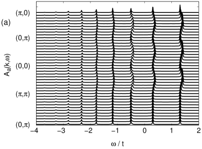
Figure 9: Spectral function as obtained in the SCBA for the effective $t_{2g}$ model (59) for a hole doped into: (a) $a$ orbital, and (b) $b$ orbital. Parameters: $J=0.4t$, $\tau=0.1t$, and peak broadening $\delta=0.01t$.

The lack of the QP dispersion in one direction, e.g. along the $a$ direction for a hole doped into the $a$ orbital, is at first instance counterintuitive: One could imagine that it should be allowed that the hole doped into the $a$ orbital switches to a neighboring site of the $B$ sublattice by the $t$ process, and then propagates freely along the $a$ axis by the three-site effective hopping $\tau$ without generating any further defects. This might lead to some dispersion in the spectra along the $k_{x}$ direction. However, the hole always has to return to the original site where it has been doped as it has to erase the defect it created in the first $t$ step when it moved to the other sublattice (otherwise, the hole annihilation operator would not permit to return to the ground state). Note that this behaviour is similar to the hole confinement in a three–site cluster as calculated for the hole doped into the $b$ orbital in the 1D model, cf. Fig. 1.notesub As a result of such processes, one finds very small incoherent (and ${\bf k}$-independent) spectral weight in the spectra of Fig. 9, which remains invisible in the present scale. This discussion demonstrates also that the spectra found for the 2D $t_{2g}$ orbital model are dominated by the 1D physics explained in Secs. II and IV.

Next, three remarks which concern the validity of our results are in order here. Firstly, note that if we skip the flavor-conserving three-site terms (62), the calculated spectral functions (not shown) reproduce the well-known ladder spectra and are equivalent to those calculated for the Ising limit of the spin $t$-$J$ model. Mar91 This means that the zig-zag-like hole trapping in the orbital case is physically similar to the standard hole trapping in the spin case (apart from the modified energy scale due to a different value of the superexchange, the ladder spectra are similar in both cases), whereas for the free hole movement obviously it matters whether the dispersion relation is 1D or 2D. Moreover, this also means that in this special case ($\tau=0$) the spectra are the same for holes doped into either of the orbitals as the Green’s functions are the same for both sublattices. However, even in this case it is not allowed to assume a priori that $A=B$ and $G_{AA}({\bf k},\omega)=G_{BB}({\bf k},\omega)$. In fact, these are two sublattices with two distinct orbital states occupied in the ground state at half filling, and each orbital has entirely different hopping geometry. This does not happen in the standard spin case with isotropic hopping, and for this reason one can eliminate there the sublattice indices.

\psfrag{a}{(a)}\psfrag{b}{(b)}\psfrag{c}{(c)}\psfrag{d}{(d)}\psfrag{e}{(e)}\psfrag{f}{(f)}\includegraphics[width=86.72267pt]{holot10a.eps}

\psfrag{a}{(a)}\psfrag{b}{(b)}\psfrag{c}{(c)}\psfrag{d}{(d)}\psfrag{e}{(e)}\psfrag{f}{(f)}\includegraphics[width=86.72267pt]{holot10b.eps}

Figure 10: (Color online) Schematic representation of two three-site terms in the $t_{2g}$ orbital model (53). Circles depict holes while horizontal (vertical) rectangles depict occupied orbitals with electrons that can move only horizontally (vertically), respectively. Processes shown in panels (a)–(c) result from forward propagation (56), while the ones shown in panels (d)–(f) and given by Eq.. (57) create a defect in the AO order with the energy cost indicated by the lines (broken bonds) in (f).

Secondly, to obtain the result shown in Fig. 9 we neglected the three-site terms with $90^{\circ}$ hopping, see Eq. (57). One may wonder whether this approximation is justified whereas the formally quite similar forward hopping term (56) is crucial and is responsible for the absence of hole confinement in the ground state with the AO order.Dag08 Hence, let us look in more detail at these two different kinds of three-site terms, shown in Fig. 10. The first (linear) hopping term (56) transports an $a$ electron along the $b$ axis over a site occupied by a $b$ electron. Such processes are responsible for the 1D coherent hole propagation. As we can see in Figs. 10(a)–(c), the AO order remains then undisturbed, so these processes determine the low-energy features in the spectra. Hopping by the other three-site term (57), shown in Fig. 10(d)–(f), involves an orbital flip at the intermediate site, destroys the AO order on six neighboring bonds, and thus costs additional energy. As two orbitals are flipped and two excited states are generated, these processes go beyond the lowest order perturbation theory, and it is consistent to neglect them in the SCBA. In any case, they could contribute only to the incoherent processes at high energy and not to the low-energy QP. Indeed, this interpretation was confirmed by exact diagonalization performed for the strong-coupling Hamiltonian (53) on $4\times 4$ and $4\times 6$ clusters, which gave the same results for the QP dispersion, no matter whether the orbital-flipping terms (57) were included or not. In addition, the QP dispersion found in the SCBA agrees with the numerical results obtained by the VCA (see below), which gives further support to the present SCBA.

Lastly, despite several other approximations made in writing down the Hamiltonian Eq. (59), the vertex part $H_{t}$ is exact, in contrast to the Ising interaction for spins.Mar91 The reason is that the constraint $C1$ mentioned above and in Ref. Mar91, , which states that a hole and a boson excitation are prohibited to occur simultaneously at the same site, cannot be violated here, because hopping $t$ is strictly 1D. This can be checked either by looking at $H_{t}$ and verifying that the projection operators $(1-\alpha^{\dagger}_{i}\alpha_{i})$ can be skipped without changing the physics, or by looking at the photoemission spectra in the limit of $J\to 0$. Whereas we did both of these checks, let us note here that for $J=0$ one obtains the incoherent spectrum with a bandwidth of $W_{\rm inc}=4\sqrt{2}t$ (not shown), which (unlike in the spin case) perfectly agrees with the RPA result $W_{\rm inc}=4\sqrt{z-2}t$ from Ref. Bri70, , where $z-2$ is the number of possible forward going steps in the model. However, still the three-site terms $H_{3s}^{(0)}$ and the orbiton terms $H_{J}$ are not exact in Eq. (59) and thus we checked the present results by comparing them with the numerical spectra obtained for the orbital Hubbard model (52) — the results are presented in the next subsection.

V.4 Comparison with numerical VCA results

Since the problem of a hole added to the background with the AO order of $t_{2g}$ orbitals cannot be solved exactly using analytic methods and the SCBA had to be employed in the last section, we used also a numerical approach. Actually, we compare the analytic results for the strong-coupling model (53) presented in Sec. V.3 with those obtained for the $t_{2g}$ Hubbard model (52) using VCA. This enables us to compare not only the methods employed but also the two models which stand for the same physics in the strongly correlated regime.

We first use the VCA to determine the staggered orbital moment in the ground state of the $t_{2g}$ orbital Hubbard model (52),

$$m_{\rm stagg}\equiv\frac{1}{N}\sum_{i}e^{i{\bf Q}\cdot{\bf R}_{i}}\left|\left\langle\tilde{n}_{ib}-\tilde{n}_{ia})\right\rangle\right|,$$ (79)

with ${\bf Q}=(\pi,\pi)$ corresponding to the 2D AO order. We compare this result to the similar ones obtained for the spin Hubbard model and for the $e_{g}$ orbital Hubbard model for a 2D plane (the strong-coupling model corrresponding to the latter situation was studied in Refs. vdB00, ; Dag07, .) As expected, $m_{\rm stagg}$ increases with decreasing $J$ (increasing $U$), see Fig. 11. For $J\to 0$ ($U\to\infty$), $m_{\rm stagg}\to 1$ for both orbital models, corresponding to the perfect (classical) 2D Ising-like order, while quantum fluctuations reduce the moment $m_{\rm stagg}$ in the spin model. We remark that the treatment of the quantum fluctuations within the VCA is far from perfect (and limited by actual cluster size), so the staggered magnetization reaches $m_{\rm stagg}\simeq 0.85$ in the limit $J\to 0$ (Fig. 11), and does not reproduce the value of $0.606$, well known from the spin-wave theory. Mat06

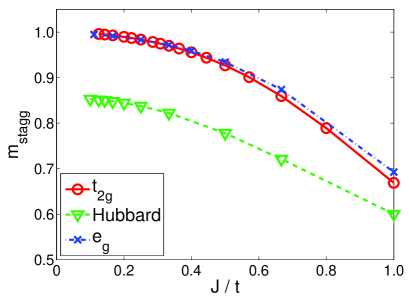
Figure 11: (Color online) Staggered magnetization $m_{\rm stagg}$ for increasing $J/t$ as obtained for the $t_{2g}$ orbital Hubbard model, spin Hubbard model (called Hubbard on the figure), and for the $e_{g}$ orbital Hubbard model, respectively.

In all three models, the staggered moment (79) obtained using the VCA decreases with decreasing $U$ (increasing $J$), see Fig. 11, because the kinetic energy can then generate more doubly occupied sites in the ground state. One finds that both the $e_{g}$ and $t_{2g}$ models give very similar results for the staggered moment, but differ strongly from the SU(2) symmetric spin model, as has been shown before in three dimensions.Fei05 However, we note that orbital order is slightly weaker for $e_{g}$ orbitals than for $t_{2g}$. This may be easily explained by the fact that the $e_{g}$ hopping is slightly smaller than $t$ for the relevant orbital states $1/\sqrt{2}(|z\rangle\pm|x\rangle)$, while all other hopping processes are frustrated by the AO order (79). Consequently, correlations have a stronger impact on $e_{g}$ electrons and induce a slightly enhanced $m_{\rm stagg}$. Finally, we would like to emphasize that the AO is 2D in all three models, in spite of the fact that the kinetic energy is strongly anisotropic in the orbital models and actually has a 1D nature in the $t_{2g}$ model, see below.

Before we analyze the spectral functions, let us recall that the VCA Aic03 is appropriate for models with on-site interactions, as for instance the present Hubbard model (52) for $t_{2g}$ orbitals, but cannot be easily implemented for models where the interacting part connects different sites, like in the $t$-$J$ (or strong-coupling) model. For the present $t_{2g}$ model (52) we use VCA with commonly usedAic03 open boundary conditions, which leads to the spectral densities depicted in Fig. 12. The results resemble very much the SCBA results of Fig. 9 for the strong-coupling model (53), suggesting that not only both models are indeed equivalent in the strongly correlated regime, but also that the implemented SCBA method of Sec. V.3 is of a very good quality. The differences between them, almost exclusively affecting high-energy features, are discussed below.

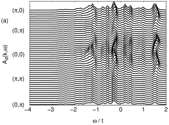
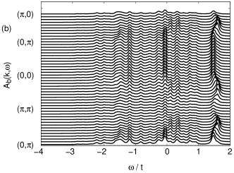
Figure 12: Spectral function $A({\bf k},\omega)$ obtained with VCA for the 2D $t_{2g}$ Hubbard model (52) for: (a) $a$ orbitals, and (b) $b$ orbitals. Parameter: $U=10t$.

On the one hand, we see that the high-energy part of the spectral density in Fig. 9 is composed of a number of peaks with a dispersion almost parallel to that of the QP state. In fact, the spectrum corresponds almost exactly to the ladder spectrum of the spin $t$-$J$ model with Ising superexchange,Kan89 ; Mar91 but with a weak dispersion added to the peaks. The peaks at higher-energy are dispersive for the same reason as the QP state: After hopping a few times by NN hopping $t$ — and creating string excitations, see Fig. 7 — the hole can exhibit coherent propagation via three-site terms, leading to the observed dispersion. On the other hand, the VCA spectrum (Fig. 12) does not show these distinct peaks and the structure of $A({\bf k},\omega)$ is richer. However, the first moments calculated in separate intervals of $\omega$ follow similar dispersions obtained for the first three peaks obtained in $A({\bf k},\omega)$ within the SCBA. Dag08

The above difference can be understood as following from the full Hilbert space used in the VCA calculations which results in excitations of doubly occupied sites, weakening of the AO order even for relatively large $U=10t$, see Fig. 11. Therefore, the spectra of Fig. 12 have more incoherent features. In addition, the three-site terms which create two orbiton excitations (57), that were neglected in the SCBA, might also influence the high-energy part of the spectrum. The difference to the SCBA results might also be due to the fact that states with longer strings including several orbital excitations, which occur when the hole moves by a few steps via $t$, cannot be directly accommodated within the 10-site cluster solved here, and cannot be reproduced with sufficient accuracy.

Apart from the differences in the high-energy part of the spectrum, we also observe differences in the spectral weight distribution (see also the detailed discussion below in Sec. V.5): In the VCA results (Fig. 12) the total weight found in photoemission part (hole excitation) strongly depends on momentum ${\bf k}$, while no such variation can be seen in the SCBA results in Fig. 9. This difference does not originate from different approximate methods used, but stems from the different models: In Hubbard-like models, the number of electron states occupied depends on the momentum ${\bf k}$.Ste91 In contrast, undoped $t$-$J$-like models have exactly one electron per site, which enforces a different sum rule and eliminates the ${\bf k}$-dependence from the photoemission part.

V.5 Discussion of quasiparticle properties

In order to get a deeper understanding of the problem mentioned in the last paragraph of Sec. V.4, let us consider first the overall spectral weight distribution obtained in the VCA calculations. It is measured by the momentum-dependent electron occupation

$$n_{\alpha}({\bf k})\equiv\left\langle c_{{\bf k}\alpha}^{\dagger}c_{{\bf k}\alpha}\right\rangle,$$ (80)

obtained for the $\alpha$-flavor in the Hubbard model, as for instance the $t_{2g}$ model (52). We recall that Eq. (52) which leads in the limit $U\gg t$ to the 2D $t_{2g}$ model (53) is rather different from the one obtained for the spin Hubbard model with the SU(2) symmetry, see Fig. 13. One may easily identify the quasi-1D dependence only on $k_{x}$ in the $b$ orbital momentum dependence $n_{b}({\bf k})$ shown in Fig. 13(a), in contrast to the 2D variation of $n_{\sigma}({\bf k})$ in the spin case with isotropic hopping of Fig. 13(b).

\psfrag{0p}[Bl]{$(0,\pi)$}\psfrag{p0}[cl]{{$(\pi,0)$}}\psfrag{pp}[Bl]{$(\pi,\pi)$}\psfrag{O}[cl]{$(0,0)$}\includegraphics[width=203.80193pt]{holot13a}

\psfrag{0p}[Bl]{$(0,\pi)$}\psfrag{p0}[cl]{{$(\pi,0)$}}\psfrag{pp}[Bl]{$(\pi,\pi)$}\psfrag{O}[cl]{$(0,0)$}\includegraphics[width=203.80193pt]{holot13b}

Figure 13: (Color online) Dependence of total weight found in the photoemission spectrum on momentum $k$ for (a) a hole inserted into the $b$ orbital of the $t_{2g}$ model (52) and (b) for a hole with spin up in the SU(2) symmetric spin Hubbard model. All data were obtained by VCA. For illustration, we added a line at $n(k)=0.5$, corresponding to the constant $n(k)$ for $t$-$J$-like models. The insets show the first quadrant of the first BZ: The arrows indicate the path taken for the main panel, the shaded area gives momenta with $n_{b}>0.5$ and $n_{\uparrow}>0.5$, respectively.

The insets in Fig. 13 show which states are occupied at $U=0$ in the two models, and indicate the difference between the isotropic 2D hopping of the spin model and the 1D kinetic energy of the orbital model. For instance, $n_{\sigma}({\bf k})=0.5$ along the $(0,\pi)--(\pi,0)$ line for spins, while it shows full variation along this line in the orbital case. In both cases, we observe strong modifications of the electron distribution with increasing $U$. For $U=0$, the states below the Fermi surface (${\bf k}\in{\cal S}_{\textrm{F}}$) are occupied and states above it (${\bf k}\not\in{\cal S}_{\textrm{F}}$) are empty. Consequently, $n_{\alpha}({\bf k})$ is given by a step function with: $n_{\alpha}({\bf k})=1$ for $k\in{\cal S}_{\textrm{F}}$ and $n_{\alpha}({\bf k})=0$ for $k\not\in{\cal S}_{\textrm{F}}$. The changes are particularly fast in the range of $U\sim 8t$; for $U>8t$ the momentum distribution function $n_{\alpha}({\bf k})$ (80) smears out and one recognizes the strong-coupling regime. However, the difference between $n_{\alpha}({\bf k}=(0,0))$ and $n_{\alpha}({\bf k}=(\pi,\pi))$ is larger in the spin model, suggesting that the correlation effects are stronger in the orbital case. Indeed, this follows from the 1D character of the kinetic energy in the orbital model. In contrast, both strong-coupling models (for spin or orbital flavors) would give at half filling a constant $n_{\alpha}({\bf k})=0.5$ even for finite $U<\infty$, although this result is strictly speaking correct only at $U=\infty$, as shown in Fig. 13.

After understanding the differences between the QP properties found in the VCA and the SCBA, we concentrate solely on the QP properties calculated using the latter method. Hence, following Ref. Mar91, , we analyze the characteristic features of the QP states in the 2D $t_{2g}$ model, such as the bandwidth $W$ and the QP spectral weight $a_{\rm QP}$. The energy of incoherent excitations (string states) is to some extent characterized by the separation between the QP state and the next (second) spectral feature at higher energy – it is called here a pseudogap $\Delta$. All these quantities increase with increasing superexchange energy $J$ ($\tau=J/4$), see Fig. 14. One finds that: (i) the bandwidth $W_{1}$ of the first QP peak, see Fig. 14(a), is proportional to $J^{2}$ for small $J$ ($J<0.7$) and to $J$ in the regime of large $J$ ($J>0.7$) — the bandwidth renormalization is here distinct from the one found either in the spin SU(2) (see Ref. Mar91, ) or in the orbital $e_{g}$ models,vdB00 (ii) the bandwidth $W_{2}$ of the second largest dispersive peak [Fig. 14(a)] is smaller than that for the first peak and tends to saturate at $W_{2}\sim 0.25t$ value for larger $J>t$ (not shown), (iii) the spectral weight $a_{\rm QP}$ of the QP peak, shown in Fig. 14(b), grows with $J$, and (iv) the pseudogap $\Delta$ shown in Fig. 14(c) grows generally like $J^{2/3}$, while for higher $J$ values some deviation from this law is observed for the ${\bf k}=(0,0)$ point. Most (but not all) of these results are qualitatively different from the ones obtained for the QP states, and their momentum dependence, in the SU(2) Heisenberg antiferromagnet. Let us now discuss the above mentioned QP properties in more detail.

Figure 14: (Color online) Quasiparticle properties obtained for the 2D $t_{2g}$ model within the SCBA for increasing superexchange $J$ (with $\tau=J/4$): (a) the bandwidth of the QP $W_{1}$ (solid line) and the second dispersive feature $W_{2}$ (dotted line), (b) the spectral weight $a_{\rm QP}$, and (c) the distance between the first two peaks in the spectra (pseudogap) $\Delta$. The solid (dashed) lines in (b) and (c) give the results for ${\bf k}=(0,0)$ [${\bf k}=(\pi/2,\pi/2)$], respectively. The light solid line in (c) indicates the $t(J/t)^{2/3}$ law (see text).

Firstly, the QP bandwidth arising from the superexchange three-site terms is renormalized as it is much smaller than the respective free value, $W\ll 2J$. Even at $J=t$, the QP bandwidth is only $W\simeq J/2$, i.e., is here reduced by a factor of 4. This is not surprising in the view of incoherent processes which ”dress” the propagating hole and increase its effective mass. Indeed, the collapse of the QP bandwidth in the regime of $J\to 0$ may be understood as following from numerous incoherent string excitations which are easy in this regime as they do not cost much energy. A similar but considerably weaker reduction of the 1D dispersion by string excitations was seen before in the centipede model, see Fig. 6(a). However, in that case the renormalization was almost linear as the length of the string excitations was limited to a single step (within one of the three-atom units along the chain), and could not further increase with decreasing $J$. In addition, the dispersion of the second peak is weaker than that of the QP. Interestingly, the bandwidth corresponding to the dispersion of the second peak in the centipede model is not only weaker than that of the QP itself, but is also renormalized in a similar way to that found for the full 2D $t_{2g}$ model. Altogether, this suggests that the bandwidth renormalization of the coherent hole propagation in the 2D $t_{2g}$ strong-coupling model follows from the creation of string states during the 1D hole propagation via three-site terms. Such processes are absent in the 1D and 2D FK model, and therefore the hole moves there freely by three-site hopping terms and the bandwidth is unrenormalized.

Secondly, in contrast to the spin $t$-$J$ model with Ising superexchange interactions,Mar91 where the QP spectral weight is independent of ${\bf k}$, it varies here with the component ($k_{x}$ or $k_{y}$) of the momentum ${\bf k}$, cf. Fig. 14 as well as Fig. 9 and 12. Similar to the spin $t$-$J$ model, the QP spectral weight is larger for the ${\bf k}$ values with the lowest QP energies than for the ones close to the maximum in QP dispersion, for instance $a_{\rm QP}(\pi/2,\pi/2)>a_{\rm QP}(0,0)$, see Fig. 14(b). Altogether, the ${\bf k}$-dependence here is however much weaker than in the spin case.Mar91 The increase of $a_{\rm QP}(\pi/2,\pi/2)$ with $J/t$ resembles the increase of the spectral weight for the low-energy peak at $k=\pi/2$ in the centipede model, see Fig. 6(b).

Finally, we address the issue of the pseudogap which separates the QP state from the first incoherent excitation. It scales almost as $t(J/t)^{2/3}$, see Fig. 14(c), in agreement with the result for the Ising spin model. Mar91 This demonstrates that in spite of the observed ${\bf k}$-dependence of the QP properties and the pseudogap itself, the pseudogap originates from string excitations similar to those generated by the hole moving in the spin background with AF order. Note also that the spectrum of the 2D model with dense distribution of incoherent maxima in the range of $J\to 0$ is qualitatively different from the 1D centipede model, shown in Fig. 5(b).

VI Photoemission spectra of vanadates and fluorides

In this Section we discuss the possible implications of the results obtained for the $t_{2g}$ orbital model of Sec. V on future experiments, and make predictions concerning the photoemission spectra of strongly correlated fluorides and vanadates. As before, we discuss the strongly correlated regime with $U\gg t$. The first important feature to consider is the interplay of the three-site hopping with the longer-range $\{t_{2},t_{3}\}$ hopping to second and third neighbors which contributes to the electronic structure and may always be expected in any realistic system (for instance, due to hybridization with oxygen orbitals). These hopping elements were neglected in both the Hubbard model (52) and in the strong-coupling model (53), but they could significantly influence the spectral weight distribution. We will see, however, that although features induced by longer-range hopping are small as long as $|t_{2(3)}|<t$, they can be clearly distinguished from the effects of three-site hopping.

The same requirements for orbital symmetry that are necessary to obtain NN hopping, as discussed in this work, also strongly restrict the range of allowed longer-range hopping terms. It is important to recall that the $d$–$d$ hopping elements involve intermediate oxygen orbitals. For next nearest neighbor (NNN) hopping, the orbital phases of the involved oxygen $2p_{\pi}$ orbitals make all terms vanish that conserve orbital flavor,Zaa93 and only orbital-flipping terms,

$$H_{\textrm{NNN}}=-t_{2}\sum_{i}\left(a^{\dagger}_{i\pm\bf{\hat{b}}}b_{i\pm\bf{\hat{a}}}+a^{\dagger}_{i\mp\bf{\hat{b}}}b_{i\pm\bf{\hat{a}}}+\textrm{h.c.}\right)\,,$$ (81)

given by hopping element $t_{2}$, are finite. With realistic parameters, we arrived at the estimation of $|t_{2}|\sim 20$ meV, i.e., $|t_{2}|\sim J/3$. Similar to the orbital flipping three-site term (57), such a hopping process disturbs the AO order stabilized by the superexchange and induces string excitations. For this reason, its impact is largely confined to the high-energy part of the spectrum and is rather small for the low-energy QP state. This can be seen in Fig. 15, where we show the spectral density for $t_{2}=0.15t$ and $J=0.4t$: While the higher energy part is somewhat affected by finite $t_{2}$, the intensity and dispersion of the low-energy QP is almost the same as obtained for $t_{2}=0$, see Fig. 12(b).

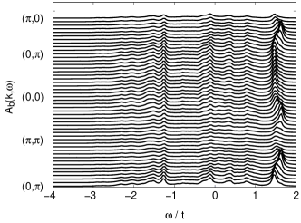
Figure 15: Spectral density $A_{b}({\bf k},\omega)$ obtained within the VCA method for a hole inserted into $b$ orbitals of the $t_{2g}$ model (52), supplemented by finite NNN hopping (81). Parameters: $U=10t$, and $t_{2}=0.15t$.

The QP dispersion could also be influenced by the third-neighbor hopping terms $t_{3}$, where the orbital symmetry leads to the same anisotropy as for NN hopping: $a$ orbitals allow only hopping along the $a$ axis, and $b$ orbitals only along the $b$ one:

$$H_{\rm t_{3}}=-t_{3}\sum_{\{imj\}\parallel a}b^{\dagger}_{i}b_{j}-t_{3}\sum_{\{imj\}\parallel b}a^{\dagger}_{i}a_{j}\;.$$ (82)

Here the unit consisting of three sites $\{imj\}$, shown in Fig. 7(a), is parallel to one of the cubic axes in the $(a,b)$ plane. In contrast to $t_{2}$ terms, these terms do not induce any string excitations but contribute only to the QP state itself, so they mix with the three-site effective hopping $\tau$. To illustrate this effect, we have chosen $t_{3}=\pm J/4$ for the spectra shown in Fig. 16. Note that the value of $|t_{3}|$ is here larger than expected in transition metal oxides, where it is in general smaller than the three-site hopping term $\tau=J/4$. The spectral density $A({\bf k},\omega)$ contains now the combined effects of the three-site terms $\propto\tau$ and third-neighbor hopping $\propto t_{3}$, and one finds that $t_{3}$, depending on its sign, can either amplify or weaken the QP dispersion which stems from the effective three-site hopping, see Fig. 16

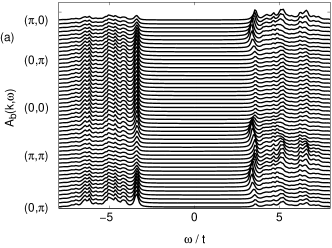
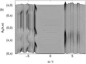
Figure 16: Photoemission [$(\omega-\mu)<0$] and inverse photoemission [$(\omega-\mu)>0$] part of the spectral density $A_{b}({\bf k},\omega)$ for a hole inserted into $b$ orbitals, obtained within VCA for the $t_{2g}$ model (52) with an additional longer-range third-neighbor hopping $t_{3}$ (82). The value $t_{3}$ was selected to suppress dispersion arising from the three-site effective hopping (56) in: (a) the hole (photoemission) sector with $t_{3}=0.1t=J/4$, and (b) in the inverse photoemission sector with $t_{3}=-0.1t=-J/4$. Parameter: $U=10t$.

From the above example we have seen that the longer-range hopping violates the particle-hole symmetry of the spectral functions. The spectra obtained for the original orbital Hubbard model (52) with NN hopping $t$ obey the particle-hole symmetry. The three-site superexchange terms arise from this model, and therefore these terms also have to follow the particle-hole symmetry. This is in marked contrast to the $t_{2}$ terms that do not respect it,Fle97 or to $t_{3}$ terms, see Fig. 16. As a result, the spectra exhibit a striking particle-hole asymmetry — reduced dispersion in the particle (inverse photoemission) sector corresponds to enhanced dispersion in the hole (photoemission) sector and vice versa.

We will show now that the above asymmetry follows indeed from the difference between the NN and NNN hopping under particle-hole transformation. While this is transparent for the Hubbard model acting in the full Hilbert space, it is somewhat subtle for the $t$–$J$-like models. Thereby we focus on the $t_{3}$ hopping which influences directly the QP dispersion. The operator for NN hopping can be transformed from $\{c_{\bf r},c^{\dagger}_{\bf r}\}$ electron operators to $\{h^{\dagger}_{\bf r},h_{\bf r}\}$ hole operators, and one arrives at an identical form for the kinetic energy, as long as a phase shift between the two sublattices is introduced:

$$h^{\dagger}_{\bf r}=(-1)^{(r_{x}+r_{y})}c_{\bf r}\,,\hskip 19.91684pth_{\bf r}=(-1)^{(r_{x}+r_{y})}c^{\dagger}_{\bf r}\,,$$ (83)

where ${\bf r}=(r_{x},r_{y})$ is the lattice site. Hopping along the $a$ axis then becomes

$$K_{x} = \sum_{\bf r}(c^{\dagger}_{\bf r}c_{{\bf r}+\hat{{\bf a}}}+c^{\dagger}_{{\bf r}+\hat{{\bf a}}}c_{\bf r})$$ (84)

$$= \sum_{\bf r}\left\{\,(-1)^{r_{x}+r_{y}}h_{\bf r}(-1)^{r_{x}+1+r_{y}}h^{\dagger}_{{\bf r}+\hat{{\bf a}}}\right.$$

$$\hskip 14.22636pt\left.+(-1)^{r_{x}+1+r_{y}}h_{{\bf r}+\hat{{\bf a}}}(-1)^{r_{x}+r_{y}}h^{\dagger}_{\bf r}\;\right\}$$

$$= -\sum_{\bf r}\left(h_{\bf r}h^{\dagger}_{{\bf r}+\hat{{\bf a}}}+h_{{\bf r}+\hat{{\bf a}}}h^{\dagger}_{\bf r}\;\right)$$

$$= \sum_{\bf r}\left(\;h^{\dagger}_{\bf r}h_{{\bf r}+\hat{{\bf a}}}+h^{\dagger}_{{\bf r}+\hat{{\bf a}}}h_{\bf r}\;\right)\;,$$

and analogously along the $b$ axis. The minus sign for one of the sublattices corresponds to a momentum shift by $\bf{q}=(\pi,\pi)$, as can be easily verified in the Fourier transform.

$$h^{\dagger}_{\bf k} = \frac{1}{N}\sum_{\bf r}\textrm{e}^{\textrm{i}\bf{kr}}(-1)^{(r_{x}+r_{y})}c_{\bf r}$$ (85)

$$= \frac{1}{N}\sum_{\bf r}\textrm{e}^{\textrm{i}(\bf{k}+\bf{q})\bf{r}}c_{\bf r}=c_{\bf{k}+\bf{q}}\,.$$

The on-site density-density interaction is not affected by the particle-hole transformation, apart from a shift in the chemical potential.

Since the three-site hopping emerges from the Hubbard-like model with NN hopping, it respects particle-hole symmetry. Hence it obeys the same rules concerning particle-hole transformation, i.e., momentum $(0,0)$ for electrons is mapped to $(\pi,\pi)$ for holes. For the third-neighbor hopping $t_{3}$ (82), however, the above transformation does not longer work, because both the creation and the annihilation operator act on the same sublattice. Instead the transformation vector would have to be ${\bf q}^{\prime}=(\pi/2,\pi/2)$. Consequently, the combined effect of explicit NNN hopping and three-site terms stemming from NN processes turns out to be strongly particle-hole asymmetric. For example, negative $t_{3}$ gives a band in the electron sector with the largest distance from the Fermi energy at momenta $(0,0)$ and $(\pi,\pi)$, and the values nearest to it at $(\pi/2,\pi/2)$, and the same is true for the three-site hopping. Consequently, the two dispersions add together and lead to increased total dispersion, see the photoemission part in Fig. 16. On the contrary, in inverse photoemission the direct NNN hopping $t_{3}$ gives a maximal distance at $(\pi/2,\pi/2)$, while maximal energy is still found at $(0,0)$ and $(\pi,\pi)$ for the three-site terms. Therefore, now $t_{3}$ and three-site hopping $\tau$ compete with each other, and the dispersion is weaker. For a particular choice of the model parameters they can even cancel each other, as shown in the inverse photoemission part in Fig. 16. Positive $t_{3}$ leads to the opposite result, see Fig. 16. Thus, even large and unphysical values of $t_{3}$ not only do not destroy the qualitative spectra predicted in the previous sections but result in asymmetry between the photoemission and inverse photoemission part of the spectra, so their contribution can easily be resolved.

The symmetry arguments leading to Eq. (81) and Eq. (82) remain valid also for systems with specific $e_{g}$ orbital degeneracy, as observed in certain fluorides with 2D AO order which involves alternating $z^{2}-y^{2}$ and $x^{2}-z^{2}$ orbitals.Wu07 In fact, the orbital model given by Eq. (53) describes also this case, as we show by a detailed derivation in the Appendix. Hence, we conclude that the photoemission and inverse photoemission spectra for the planar vanadium oxide Sr₂VO₄ and for the planar K₂CuF₄ or Cs₂AgF₄ fluorides should be qualitatively similar to the spectral functions shown in Figs. 9 or 12.

VII Summary and Conclusions

In this paper we analyzed only the orbital sector of the superexchange, which decides about the hole dynamics when spins are polarized in the FM ground state. We discussed all possible situations (see below) where the orbital symmetry leads to the purely Ising superexchange in one and two dimensions. Exceptions from this rule are numerous systems with $e_{g}$ orbital degrees of freedom,vdB99 ; Dag01 ; Fei99 or FM chains with two active orbitals,Kha01 ; Sir08 but we also provided examples of $e_{g}$ systems with Ising superexchange.

The 1D Hubbard-like model with two orbital flavors, but only one of them participating in NN hopping, served to explain the general principles and consequences of the Ising-like superexchange. Besides, this model stands for several physically relevant situations, including electrons moving within either $e_{g}$ or $t_{2g}$ orbitals in one dimension, and the 1D FK model. We have shown that, particularly in all these cases, the relevant strong-coupling model has to include the three-site effective hopping. When both interorbital hopping and orbital-flip processes in the superexchange are absent, the three-site hopping term which arises from superexchange is crucial and is the only source of coherent hole propagation.

We have shown that the 2D FK model with one immobile ($f$) and one mobile ($d$) orbital has many common features with the 1D model. In both cases one finds only one dispersive mode for a hole inserted into the mobile orbital, and two non-dispersive modes for a hole doped in the immobile orbital. This latter hole excitation creates a trapped polaron, with the hole confined within a cluster consisting of a central site and its nearest neighbors (i.e., three sites in the 1D model, and five sites in the 2D model). While the hole can in principle escape from the polaron via three-site hopping process, we have shown that such processes have only very low spectral weight in the realistic regime of parameters, and thus the hole remains de facto trapped inside the polaron. In contrast to this almost perfectly localized hole, a hole in the mobile orbital propagates freely, and its dispersion which originates from the three-site hopping is unrenormalized. Therefore, the two inequivalent orbital flavors behave in the FK models in a radically different way, and decouple from each other (interacting only by the on-site Coulomb interaction $U$, which stabilizes the AO ground state).

The model relevant for the 2D orbital physics in transition metal oxides leads, however, to qualitatively different results. In the 2D $t_{2g}$ orbital model, which is also applicable to the AO state formed by $e_{g}$ orbitals in fluorides (see the Appendix), electrons do not separate into those confined to either sublattice (occupied by orbitals of particular symmetry in the ground state with AO order), but may delocalize over the lattice and thereby undergo incoherent scattering on the orbital excitations, which strongly renormalizes and reduces the dispersion of the QP states. These QP states arise at half filling in the regime of large Coulomb interaction $U$, when a hole (electon) is added to the ground state with AO order. While electron hopping is of the purely 1D character, it selects by symmetry possible three-site processes, which are responsible for the QP dispersion. Therefore, the dispersion of the QP state depends on the considered orbital and is again 1D, with a hole propagating coherently along the two crystal axes for the two orbitals.

We emphasize that the mechanism of coherent hole propagation which occurs in the 2D $t_{2g}$ orbital model is completely different from the one known in the spin case. In orbital systems (with conserved orbital flavors) it originates entirely from the three-site hopping processes, similar to hole propagation in the 1D or 2D FK model. But unlike in the latter models, in the 2D $t_{2g}$ case the QP bandwidth is strongly reduced from the value given by the amplitude of bare three-site hopping. We have explained this renormalization as following from incoherent string excitations which dress the coherent propagation and do not contribute additional momentum dependence. As a special case, we have discussed the subtle interplay between the coherent hole propagation and string excitations in the 1D centipede model, where polaronic hole confinement competes with coherent propagation along the chain, and which to some extent resembles the realistic 2D $t_{2g}$ case.

We discussed the impact of realistic longer-range hopping terms (as expected in real materials such as vanadates or fluorides), and found that the second neighbor terms are frustrated in the ground state with AO order – these processes would flip the orbital flavor, and are therefore suppressed at low energy, not affecting the QP dispersion. In contrast, third-neighbor hopping processes conserve orbital flavor and lead to a pronounced particle-hole asymmetry in the spectral weight distribution. In both cases, the 1D character of hole propagation which follows from the symmetry of involved orbitals, survives and determines the character of the spectral density at low energy.

In summary, we have demonstrated that orbital models with Ising superexchange describe a broad class of interesting phenomena. Spectral features resulting from such models exhibit weak momentum dependence and are fundamentally different from those known from the the spin case with the SU(2)-symmetric superexchange. The predictions of the theory presented in this paper provide an experimental challenge for the transition metal oxides with orbital degrees of freedom, where similar features could possibly be observed in FM planes with AO order.

Appendix A Strong-coupling model for fluorides

Here we show that the model developed in Sec. V may also be applied to certain fluorides with FM planes and AO order. In contrast to the $t_{2g}$ orbitally degenerate systems, in the systems with $e_{g}$ orbital degeneracy the lattice distortions in the cubic phases are usually quite large. In particular, the static distortions may counteract to some extent the AO order favored by the superexchange interactions, as e.g. in undoped manganites $R$MnO₃, Fei99 or fluorides Cs₂AgF₄.Wu07 However, the crystal field does not suppress the orbital order present in these systems but instead it only modifies the occupied orbitals which form the AO state. They have to be optimized in a microscopic model by choosing particular linear combinations of the $e_{g}$ orbitals, which form the AO order, in order to fit best to the superposition of the superexchange and the Jahn-Teller terms generated by ligand fields.Ole05 In certain situations this ”modification” could be quite substantial and could even lead to such a selection of such $e_{g}$ orbitals that the resulting state is modified to a ferro-type orbital order. vdB99

At finite crystal field splitting $\propto E_{z}$, it is convenient to describe the changes in the occupied orbital states by making two complementary transformations at both sublattices, vdB99 rotating the orbitals by an angle $\theta=\frac{\pi}{4}-\phi$ on sublattice $A$, and by an angle $\theta=\frac{\pi}{4}+\phi$ on sublattice $B$, so that the relative angle between the occupied orbitals is $\frac{\pi}{2}-2\phi$ and decreases with increasing $\phi$, i.e., with increasing $E_{z}$,

$$\left(\begin{array}[]{c}|\mu\rangle_{i}\\ |\nu\rangle_{i}\end{array}\right)\!=\!\left(\begin{array}[]{cc}\ \ \cos(\frac{\pi}{4}-\phi)&\sin(\frac{\pi}{4}-\phi)\\ -\sin(\frac{\pi}{4}-\phi)&\cos(\frac{\pi}{4}-\phi)\end{array}\right)\!\left(\begin{array}[]{c}|\mbox{z}\rangle_{i}\\ |\mbox{x}\rangle_{i}\end{array}\right),$$ (86)

$$\left(\begin{array}[]{c}|\mu\rangle_{j}\\ |\nu\rangle_{j}\end{array}\right)\!=\!\left(\begin{array}[]{cc}\ \ \cos(\frac{\pi}{4}+\phi)&\sin(\frac{\pi}{4}+\phi)\\ -\sin(\frac{\pi}{4}+\phi)&\cos(\frac{\pi}{4}+\phi)\end{array}\right)\!\left(\begin{array}[]{c}|\mbox{z}\rangle_{j}\\ |\mbox{x}\rangle_{j}\end{array}\right),$$ (87)

where the ”old” orthogonal (basis) orbitals are defined as $|\mbox{x}\rangle_{i}=\frac{1}{\sqrt{2}}|x^{2}-y^{2}\rangle_{i}$ and $|\mbox{z}\rangle_{i}=\frac{1}{\sqrt{6}}|3z^{2}-r^{2}\rangle_{i}$ for every sublattice site $i$. Due to the above transformation the AO order is formed now by $|\mu\rangle_{i}$ and $|\nu\rangle_{j}$ occupied orbitals at sublattices, $i\in A$ and $j\in B$, respectively. Let us stress that although the transformation defined by Eqs. (86–87) is orthogonal this does not mean that orbitals on different sublattices, such as e.g. the occupied orbitals $|\mu\rangle_{i}$ and $|\nu\rangle_{j}$, are orthogonal for any arbitrary angle $\phi$.

For the 2D FM systems with active $e_{g}$ orbitals which are considered here, the relation between the crystal field $E_{z}$ and the optimal orbital configuration defined by the angle $\phi$ [see Eqs. (12) and (13) of Ref. vdB99, ] is given by:

$$E_{z}=4J\sin 2\phi,$$ (88)

where $J$ is the superexchange constant. In the case of fluorides such as Cs₂AgF₄ (Ref. Wu07, ) or K₂CuF₄ (Ref. Hid83, ) discussed here, the filling is one $e_{g}$ electron per site and the crystal field would select the angle $\phi=\pi/12$ (for the reason of looking at this angle see below) since the convenient basis adapted to the actual AO order looks as follows:

$$\forall\,i\in A:\ \left|\mu\left(\phi=\frac{\pi}{12}\right)\right\rangle_{i}=\frac{1}{\sqrt{2}}|y^{2}-z^{2}\rangle_{i}\equiv|x\rangle_{i}\,,$$

$$\ \left|\nu\left(\phi=\frac{\pi}{12}\right)\right\rangle_{i}=\frac{1}{\sqrt{6}}|3x^{2}-r^{2}\rangle_{i}\equiv|z\rangle_{i}\,,$$

$$\forall\,j\in B:\ \ \left|\mu\left(\phi=\frac{\pi}{12}\right)\right\rangle_{j}=\frac{1}{\sqrt{6}}|3y^{2}-r^{2}\rangle_{j}\equiv|z\rangle_{j}\,,$$

$$\ \left|\nu\left(\phi=\frac{\pi}{12}\right)\right\rangle_{j}=\frac{1}{\sqrt{2}}|x^{2}-z^{2}\rangle_{j}\equiv|x\rangle_{j}\,,$$ (89)

where the occupied (empty) orbitals for this type of AO order are denoted as $|x\rangle$ ($|z\rangle$) on both sublattices.

The reason why these particular pairs of basis orbitals (A) are interesting here is that this is the only choice of occupied $e_{g}$ flavors which forms a two-sublattice AO order with the interorbital hopping between occupied orbitals vanishing by symmetry, and where the interactions described by pseudospin operators do not allow for any quantum fluctuations. This resembles the $t_{2g}$ case discussed in this paper. There is, however, one subtle difference: two occupied $\{|x\rangle_{i},|x\rangle_{j}\}$ orbitals on sublattices $A$ and $B$ are not orthogonal and do not form the global basis in the $e_{g}$ orbital space. The choice made in Eq. (A) means that we consider two different pairs of orbitals for both sublattices, and the interorbital hopping between the unoccupied orbitals is also rather small but remains finite.noteint Hence, the respective strong-coupling Hamiltonian is richer than the one for the $t_{2g}$ case and we need to check under which conditions it can be reduced to a similar polaron Hamiltonian as Eq. (59).

The $e_{g}$ orbital $t$-$J$ Hamiltonian for the FM planes without the three-site terms but including the crystal field was given e.g. in Ref. Bal02, . Here we rewrite the kinetic term in a slightly different form (there it was written already using the polaron representation) and substitute $\phi=\pi/12$ to obtain:

$${\cal H}_{e_{g}}=H_{t}+H_{J}+H_{z}\,,$$ (90)

where

$$H_{t} = -\frac{1}{2}t\sum_{i}(\tilde{z}^{\dagger}_{i}\tilde{z}_{i+\hat{a}}+\tilde{z}^{\dagger}_{i}\tilde{z}_{i+\hat{b}}+\mbox{h.c.})$$ (91)

$$- \frac{\sqrt{3}}{2}t\sum_{i\ \in A}(\tilde{z}^{\dagger}_{i}\tilde{x}_{i+\hat{a}}+\tilde{z}^{\dagger}_{i}\tilde{x}_{i+\hat{b}}+\mbox{h.c.})$$

$$- \frac{\sqrt{3}}{2}t\sum_{i\ \in B}(\tilde{x}^{\dagger}_{i}\tilde{z}_{i+\hat{a}}+\tilde{x}^{\dagger}_{i}\tilde{z}_{i+\hat{b}}+\mbox{h.c.})\;,$$

$$H_{J} = \frac{1}{2}J\sum_{\langle ij\rangle||\hat{a}}\left(T^{z}_{i}T^{z}_{j}+\sqrt{3}T^{z}_{i}T^{x}_{j}\right)$$ (92)

$$+ \frac{1}{2}J\sum_{\langle ij\rangle||\hat{b}}\left(T^{z}_{i}T^{z}_{j}-\sqrt{3}T^{x}_{i}T^{z}_{j}\right)\;,$$

$$H_{z} = -\frac{1}{4}J\sum_{i\in A}(T^{z}_{i}+\sqrt{3}T^{x}_{i})$$ (93)

$$+ \frac{1}{4}J\sum_{i\in B}(T^{z}_{i}-\sqrt{3}T^{x}_{i})\;.$$

Here $T^{z}_{i}=\frac{1}{2}(\tilde{n}_{iz}-\tilde{n}_{ix})$ for $i\in A$, $T^{z}_{j}=\frac{1}{2}(\tilde{n}_{jx}-\tilde{n}_{jz})$ for $j\in B$, and $T^{x}_{i}=\frac{1}{2}(\tilde{x}^{\dagger}_{i}\tilde{z}_{i}+\tilde{z}^{\dagger}_{i}\tilde{x}_{i})$ for every site $i$, see Ref. vdB99, . As before, a tilde above a fermion operator indicates that the Hilbert space is restricted to unoccupied and singly occupied sites, e.g. $\tilde{x}^{\dagger}_{i}=x_{i}^{\dagger}(1-n_{iz})$. The last term $H_{z}$ represents the above mentioned crystal field with the strength of the interaction written according to Eq. (88) with $\phi=\pi/12$.

However, we are not aware of any work where the three-site terms complementing such a $t$-$J$ model have been derived. We use second again order perturbation theoryCha77 ; Esk94 applied to the Hubbard model for spinless $e_{g}$ electrons in a FM plane,Fei05 with the basis rotated by $\phi=\pi/12$, following Eqs. (12) and (13) of Ref. vdB99, . This leads to the following three-site terms for the $e_{g}$ strong-coupling model (with $\phi=\pi/12$):

$$H_{\tau}=H^{a}_{\tau}+H^{b}_{\tau}+H^{ab}_{\tau},$$ (94)

where

$$H^{a}_{\tau}= - \!\!\frac{1}{4}\tau\sum_{i\in A}\Big{[}\tilde{z}^{\dagger}_{i-\hat{a}}\tilde{n}_{ix}\tilde{z}_{i+\hat{a}}+\underline{3\tilde{x}^{\dagger}_{i-\hat{a}}\tilde{n}_{ix}\tilde{x}_{i+\hat{a}}}+\underline{\underline{\sqrt{3}\tilde{x}^{\dagger}_{i-\hat{a}}\tilde{n}_{ix}\tilde{z}_{i+\hat{a}}}}+\underline{\underline{\sqrt{3}\tilde{z}^{\dagger}_{i-\hat{a}}\tilde{n}_{ix}\tilde{x}_{i+\hat{a}}}}+\mbox{h.c.}\Big{]}$$ (95)

$$- \frac{1}{4}\tau\sum_{i\in B}\Big{[}\tilde{z}^{\dagger}_{i-\hat{a}}\tilde{n}_{ix}\tilde{z}_{i+\hat{a}}+3\tilde{z}^{\dagger}_{i-\hat{a}}\tilde{n}_{iz}\tilde{z}_{i+\hat{a}}-\sqrt{3}\tilde{z}^{\dagger}_{i-\hat{a}}\tilde{z}^{\dagger}_{i}\tilde{x}_{i}\tilde{z}_{i+\hat{a}}-\sqrt{3}\tilde{z}^{\dagger}_{i-\hat{a}}\tilde{x}^{\dagger}_{i}\tilde{z}_{i}\tilde{z}_{i+\hat{a}}+\mbox{h.c.}\Big{]}\,,$$

$$H^{b}_{\tau} = -\frac{1}{4}\tau\sum_{i\in A}\Big{[}\tilde{z}^{\dagger}_{i-\hat{b}}\tilde{n}_{ix}\tilde{z}_{i+\hat{b}}+3\tilde{z}^{\dagger}_{i-\hat{b}}\tilde{n}_{iz}\tilde{z}_{i+\hat{b}}-\sqrt{3}\tilde{z}^{\dagger}_{i-\hat{b}}\tilde{z}^{\dagger}_{i}\tilde{x}_{i}\tilde{z}_{i+\hat{b}}-\sqrt{3}\tilde{z}^{\dagger}_{i-\hat{b}}\tilde{x}^{\dagger}_{i}\tilde{z}_{i}\tilde{z}_{i+\hat{b}}+\mbox{h.c.}\Big{]}$$ (96)

$$- \frac{1}{4}\tau\sum_{i\in B}\Big{[}\tilde{z}^{\dagger}_{i-\hat{b}}\tilde{n}_{ix}\tilde{z}_{i+\hat{b}}+\underline{3\tilde{x}^{\dagger}_{i-\hat{b}}\tilde{n}_{ix}\tilde{x}_{i+\hat{b}}}+\underline{\underline{\sqrt{3}\tilde{x}^{\dagger}_{i-\hat{b}}\tilde{n}_{ix}\tilde{z}_{i+\hat{b}}}}+\underline{\underline{\sqrt{3}\tilde{z}^{\dagger}_{i-\hat{b}}\tilde{n}_{ix}\tilde{x}_{i+\hat{b}}}}+\mbox{h.c.}\Big{]}\,,$$

$$H^{ab}_{\tau} = -\frac{1}{4}\tau\sum_{i\in A}\Big{[}\tilde{z}^{\dagger}_{i\pm\hat{a}}\tilde{n}_{ix}\tilde{z}_{i\pm\hat{b}}-3\tilde{x}^{\dagger}_{i\pm\hat{a}}\tilde{x}^{\dagger}_{i}\tilde{z}_{i}\tilde{z}_{i\pm\hat{b}}+\underline{\underline{\sqrt{3}\tilde{x}^{\dagger}_{i\pm\hat{a}}\tilde{n}_{ix}\tilde{z}_{i\pm\hat{b}}}}-\sqrt{3}\tilde{z}^{\dagger}_{i\pm\hat{a}}\tilde{x}^{\dagger}_{i}\tilde{z}_{i}\tilde{z}_{i\pm\hat{b}}$$ (97)

$$+ \tilde{z}^{\dagger}_{i\pm\hat{a}}\tilde{n}_{ix}\tilde{z}_{i\mp\hat{b}}-3\tilde{x}^{\dagger}_{i\pm\hat{a}}\tilde{x}^{\dagger}_{i}\tilde{z}_{i}\tilde{z}_{i\mp\hat{b}}+\underline{\underline{\sqrt{3}\tilde{x}^{\dagger}_{i\pm\hat{a}}\tilde{n}_{ix}\tilde{z}_{i\mp\hat{b}}}}-\sqrt{3}\tilde{z}^{\dagger}_{i\pm\hat{a}}\tilde{x}^{\dagger}_{i}\tilde{z}_{i}\tilde{z}_{i\mp\hat{b}}+\mbox{h.c.}\Big{]}$$

$$- \frac{1}{4}\tau\sum_{i\in B}\Big{[}\tilde{z}^{\dagger}_{i\pm\hat{a}}\tilde{n}_{ix}\tilde{z}_{i\pm\hat{b}}-3\tilde{z}^{\dagger}_{i\pm\hat{a}}\tilde{z}^{\dagger}_{i}\tilde{x}_{i}\tilde{x}_{i\pm\hat{b}}+\underline{\underline{\sqrt{3}\tilde{z}^{\dagger}_{i\pm\hat{a}}\tilde{n}_{ix}\tilde{x}_{i\pm\hat{b}}}}-\sqrt{3}\tilde{z}^{\dagger}_{i\pm\hat{a}}\tilde{z}^{\dagger}_{i}\tilde{x}_{i}\tilde{z}_{i\pm\hat{b}}$$

$$+ \tilde{z}^{\dagger}_{i\pm\hat{a}}\tilde{n}_{ix}\tilde{z}_{i\mp\hat{b}}-3\tilde{z}^{\dagger}_{i\pm\hat{a}}\tilde{z}^{\dagger}_{i}\tilde{x}_{i}\tilde{x}_{i\mp\hat{b}}+\underline{\underline{\sqrt{3}\tilde{z}^{\dagger}_{i\pm\hat{a}}\tilde{n}_{ix}\tilde{x}_{i\mp\hat{b}}}}-\sqrt{3}\tilde{z}^{\dagger}_{i\pm\hat{a}}\tilde{z}^{\dagger}_{i}\tilde{x}_{i}\tilde{z}_{i\mp\hat{b}}+\mbox{h.c.}\Big{]}\,.$$

Here we underlined (doubly underlined) terms which do not require orbital excitations (require orbital excitations), respectively, i.e.

$$H^{(0)}_{\tau}=\underline{H_{\tau}},\hskip 28.45274ptH^{(1)}_{\tau}=\underline{\underline{H_{\tau}}}.$$ (98)

Next, we perform the same standard transformation to obtain the polaron Hamiltonian from the strong-coupling model Mar91 for the lightly doped ordered states as done in Sec. V.3, i.e. we introduce boson operators $\alpha_{i}$ (orbitons) and fermion operators $h_{i}$ (holons) which are related to the $x_{i}$ and $z_{i}$ operators in the following way:

$$\tilde{x}^{\dagger}_{i}\equiv h_{i}(1-\alpha^{\dagger}_{i}\alpha_{i}),\hskip 28.45274pt\tilde{z}^{\dagger}_{i}\equiv h_{i}\alpha_{i}^{\dagger}.$$ (99)

Please note, however, that here we did not have to perform rotation of the pseudospins since we defined distinct electron operators for the occupied and empty orbitals, cf. Eq. (A).

Again we implement a linear orbital-wave approximationvdB99 (we keep only linear terms in orbiton operators) and we skip $(1-h^{\dagger}_{i}h_{i})$ operators (which in fact is not an approximation if there is only one hole in the entire plane). This means that e.g. the three-site terms are reduced only to the terms which were either underlined or doubly underlined in Eqs. (95)–(97), i.e. to either $H^{(0)}_{\tau}$ or $H^{(1)}_{\tau}$. Here, however, we have to use yet another approximation which was unnecessary for the $t_{2g}$ model: we skip terms $H^{(1)}_{\tau}$ which were absent in Sec. V.2. This approximation is allowed since these terms contribute to the vertex as $\propto\tau$ and not as $\propto t$, resulting typically in much reduced energy scale for the new vertex contributions. Furthermore, we showed in Sec. VI that such terms [cf. Eq. (82) and Fig. 15] do not change the energy of the QP and merely modify the incoherent spectrum. Eventually, we arrive at the polaron Hamiltonian for the holes doped into the $e_{g}$ orbitals of the fluorides, with the hopping terms:

$$H_{t} = \sqrt{3}t\frac{1}{\sqrt{N}}\sum_{{\bf k},{\bf q}}\left\{\cos(k_{x}-q_{x})h^{\dagger}_{{\bf k}A}h_{{\bf k}-{\bf q},B}\alpha_{{\bf q}A}\right.$$ (100)

$$+ \left.\cos(k_{y}\!-\!q_{y})h^{\dagger}_{{\bf k}B}h_{{\bf k}-{\bf q},A}\alpha_{{\bf q}B}+{\rm h.c.}\right\}\,,$$

$$H^{(0)}_{\tau} = \frac{3}{2}\tau\sum_{k}\left\{\cos(2k_{y})h_{{\bf k}A}^{\dagger}h_{{\bf k}A}+\cos(2k_{x})h_{{\bf k}B}^{\dagger}h_{{\bf k}B}\right\}\,,$$

and the remaining terms resulting in the energy renormalization

$$H_{J}+H_{z}=\frac{3}{4}J\sum_{k}\left(\alpha_{{\bf k}A}^{\dagger}\alpha_{{\bf k}A}+\alpha_{{\bf k}B}^{\dagger}\alpha_{{\bf k}B}\right)\,.$$ (102)

Therefore, the Hamiltonian given by Eqs. (100)–(102) reduces to the polaron Hamiltonian (59) after substituting $\sqrt{3}t/2\rightarrow t$, and consequently $3J/4\rightarrow J$ and $3\tau/4\rightarrow\tau$. This substitution stems from the different definitions of the hopping $t$ in the $e_{g}$ and in the $t_{2g}$ systems — in the former case it is the $(dd\sigma)$ hopping between the $3z^{2}-r^{2}$ orbitals along the $\hat{c}$ direction, whereas in the latter case it is the hopping element between a pair of active $t_{2g}$ orbitals, e.g. $yz$ orbitals in the ($a,b)$ plane.

In summary, we have shown that the Hamiltonian given by Eqs. (100)–(102) provides the framework to analyze the behavior of certain lightly doped $e_{g}$ systems, with FM planes and AO order which suppresses the interorbital hopping between occupied orbitals. Its equivalence to the polaron model (59) demonstrates that the results obtained and discussed in Sec. V should also apply to the case of a hole doped into the fluoride plane with the AO ordered $e_{g}$ orbitals.

References

- (1) M. Imada, A. Fujimori, and Y. Tokura, Rev. Mod. Phys. 70, 1039 (1998).
- (2) L. N. Bulaevski, E. L. Nagaev, and D. I. Khomskii, Sov. Phys. JETP 27, 836 (1968).
- (3) S. Schmitt-Rink, C. M. Varma, and A. E. Ruckenstein, Phys. Rev. Lett. 60, 2793 (1988).
- (4) C. L. Kane, P. A. Lee, and N. Read, Phys. Rev. B 39, 6880 (1989).
- (5) G. Martínez and P. Horsch, Phys. Rev. B 44, 317 (1991).
- (6) J. van den Brink, New J. Phys. 6, 201 (2004).
- (7) J. van den Brink, P. Horsch, F. Mack, and A. M. Oleś, Phys. Rev. B59, 6795 (1999).
- (8) E. Dagotto, T. Hotta, and A. Moreo, Phys. Rep. 344, 1 (2001).
- (9) L. F. Feiner and A. M. Oleś, Phys. Rev. B59, 3295 (1999).
- (10) M. Daghofer, A. M. Oleś, D. C. Neuber, and W. von der Linden, Phys. Rev. B 73, 104451 (2006); Phys. Stat. Solidi B 243, 277 (2006); M. Daghofer and A. M. Oleś, Acta Phys. Polon. A 111, 497 (2007).
- (11) P. Horsch, J. Jaklič, and F. Mack, Phys. Rev. B59, 6217 (1999).
- (12) J. Zaanen and A. M. Oleś, Phys. Rev. B48, 7197 (1993).
- (13) L. F. Feiner and A. M. Oleś, Phys. Rev. B71, 144422 (2005).
- (14) J. van den Brink, P. Horsch, and A. M. Oleś, Phys. Rev. Lett. 85, 5174 (2000).
- (15) M. Daghofer, K. Wohlfeld, A. M. Oleś, E. Arrigoni, and P. Horsch, Phys. Rev. Lett. 100, 066403 (2008).
- (16) K. A. Chao, J. Spałek, and A. M. Oleś, J. Phys. C 10, L271 (1977); Phys. Rev. B18, 3453 (1978).
- (17) P. Wróbel, W. Suleja, and R. Eder, Phys. Rev. B78, 064501 (2008).
- (18) We use here the pseudospin operators to represent orbital pseudospins.
- (19) J. K. Freericks, Phys. Rev. B47, 9263 (1993); J. K. Freericks and V. Zlatić, Rev. Mod. Phys. 75, 1333 (2003).
- (20) K. W. Becker, S. Sykora, and V. Zlatić, Phys. Rev. B75, 075101 (2007).
- (21) M. M. Maśka and K. Czajka, Phys. Rev. B74, 035109 (2006).
- (22) J. K. Freericks, V. M. Turkowski, and V. Zlatić, Phys. Rev. B71, 115111 (2005).
- (23) J. Matsuno, Y. Okimoto, M. Kawasaki, and Y. Tokura, Phys. Rev. Lett. 95, 176404 (2005).
- (24) Y. Imai, I. Solovyev, and M. Imada, Phys. Rev. Lett. 95, 176405 (2005).
- (25) A. Nozaki, H. Yoshikawa, T. Wada, H. Yamauchi, and S. Tanaka, Phys. Rev. B 43, 181 (1991).
- (26) D. Jaksch and P. Zoller, Ann. Phys. 315, 52 (2005).
- (27) T. Muller, S. Folling, A. Widera, and I. Bloch, Phys. Rev. Lett. 99, 200405 (2007); E. Zhao and W. V. Liu, ibid. 100, 160403 (2008); C. Wu, ibid. 100, 200406 (2008).
- (28) M. Hidaka, K. Inoue, I. Yamada, and P. J. Walker, Physica B 121, 343 (1983).
- (29) H. Wu and D. I. Khomskii, Phys. Rev. B76, 155115 (2007).
- (30) S. E. McLain, M. R. Dolgos, D. A. Tennant, J. F. C. Turner, T. Barnes, T. Proffen, B. C. Sales, and R. I. Bewley, Nature Mater. 5, 561 (2006).
- (31) J. Fujioka, S. Miyasaka, and Y. Tokura, Phys. Rev. B77, 144402 (2008).
- (32) We cannot exclude that models with Ising superexchange could possibly be relevant also for frustrated lattices but there a coherent quasiparticle behavior is much harder to obtain, see D. Poilblanc, Phys. Rev. Lett. 93, 197204 (2004).
- (33) H. Eskes and A. M. Oleś, Phys. Rev. Lett. 73, 1279 (1994); H. Eskes, A. M. Oleś, M. B. J. Meinders, and W. Stephan, Phys. Rev. B50, 17980 (1994).
- (34) K. J. von Szczepanski, P. Horsch, W. Stephan, and M. Ziegler, Phys. Rev. B41, 2017 (1990). J. Bała, A. M. Oleś, and J. Zaanen, ibid. 52, 4597 (1995).
- (35) S. A. Trugman, Phys. Rev. B37, 1597 (1988).
- (36) E. Dagotto, Rev. Mod. Phys. 66, 763 (1994); M. Brunner, F. F. Assaad, and A. Muramatsu, Phys. Rev. B62, 15480 (2000). M. Bejas, A. Greco, and A. Foussats, ibid. 73, 245104 (2006).
- (37) M. Potthoff, M. Aichhorn, and C. Dahnken, Phys. Rev. Lett. 91, 206402 (2003).
- (38) C. Gros and R. Valentí, Phys. Rev. B48, 418 (1993).
- (39) M. M. Maśka, Phys. Rev. B57, 8755 (1998)
- (40) D. Sénéchal, D. Perez, and M. Pioro-Ladrière, Phys. Rev. Lett. 84, 522 (2000).
- (41) M. Potthoff, Eur. Phys. J. B 36, 335 (2003).
- (42) M. Daghofer, A. M. Oleś, and W. von der Linden, Phys. Rev. B 70, 184430 (2004); Phys. Stat. Solidi B 242, 311 (2005).
- (43) W. F. Brinkman and T. M. Rice, Phys. Rev. B2, 1324 (1970).
- (44) Note that even in the – models with purely Ising-like interaction a complete summation of the self-energy can only be performed when a hole creates just a finite (and preferably small) number of defects in an infinite lattice. This is the reason why the RPA works well both for the 1D spin – model with only Ising interaction between the spins, see the appendix in J. Smakov, A. L. Chernyshev, and S. R. White, Phys. Rev. B76, 115106 (2007), and in the 1D spinless Hubbard-Wigner model with nearest neighbor repulsion [M. Daghofer and P. Horsch, Phys. Rev. B75, 125116 (2007)].
- (45) P. M. R. Brydon, Phys. Rev. B77, 045109 (2008).
- (46) M. Daghofer, W. Koller, H. G. Evertz, and W. von der Linden, J. Phys.: Condens. Matter 16, 5469 (2004).
- (47) For a minority of sites on a square lattice with AO order this number is equal to or .
- (48) G. Khaliullin and S. Maekawa, Phys. Rev. Lett. 85, 3950 (2000); G. Khaliullin, P. Horsch, and A. M. Oleś, ibid. 86, 3879 (2001).
- (49) A. M. Oleś, G. Khaliullin, P. Horsch, and L. F. Feiner, Phys. Rev. B72, 214431 (2005).
- (50) The Green’s function does not show new qualitative features as compared with the solution obtained for the 1D orbital chain of Sec. II.
- (51) P. Horsch, G. Khaliullin, and A. M. Oleś, Phys. Rev. Lett. 91, 257203 (2003); P. Horsch, A. M. Oleś, L. F. Feiner, and G. Khaliullin, ibid. 100, 167205 (2008).
- (52) D. I. Khomskii and M. V. Mostovoy, J. Phys. A 36, 9197 (2003).
- (53) One can also sum instead over values in the reduced Brillouin zone, but then one has to replace by everywhere before summations.
- (54) There is however some subtlety related to this statement. In the 1D model there are actually two interrelated reasons why the hole cannot move coherently when doped into the orbital: (i) the creation of the defect after the first step which has to be erased by the hole before the hole itself is annihilated, and (ii) the fact that this defect blocks the hole motion by three-site terms in one direction. However, in the SCBA treatment the latter constraint is neglected [as we skipped projection operators in the three-site terms when deriving the effective Hamiltonian (59)], so it is the point (i) which suffices alone to confine the hole.
- (55) D. C. Mattis, The Theory of Magnetism Made Simple (World Scientific, Singapore, 2006).
- (56) W. Stephan and P. Horsch, Phys. Rev. Lett. 66, 2258 (1991).
- (57) M. Fleck, A. M. Oleś, and L. Hedin, Phys. Rev. B56, 3159 (1997).
- (58) J. Sirker and G. Khaliullin, Phys. Rev. B67, 100408(R) (2003); J. Sirker, A. Herzog, A. M. Oleś, and P. Horsch, Phys. Rev. Lett. 101, 157204 (2008).
- (59) The physical reason for this is that finite crystal field cannot fully eliminate the interorbital hopping.
- (60) J. Bała and A. M. Oleś, Phys. Rev. B62, R6085 (2000); J. Bała, A. M. Oleś, and P. Horsch, ibid. 65, 134420 (2002).