Smeared quantum phase transition in the dissipative random quantum Ising model

Abstract

We investigate the quantum phase transition in the random transverse-field Ising model under the influence of Ohmic dissipation. To this end, we numerically implement a strong-disorder renormalization-group scheme. We find that Ohmic dissipation destroys the quantum critical point and the associated quantum Griffiths phase by smearing. Our results quantitatively confirm a recent theory [Phys. Rev. Lett. 100, 240601 (2008)] of smeared quantum phase transitions.

,

1 Introduction

The presence of impurities, defects, or other types of quenched disorder can qualitatively change the properties of a continuous phase transition. At thermal transitions, this is controlled by the Harris criterion [1]: If a clean critical point violates the inequality $\nu>2/d$ where $\nu$ is the correlation length exponent and $d$ is the space dimensionality, it is perturbatively unstable against weak disorder. The generic result of adding disorder to such a system is a new critical point with different critical exponents but conventional power-law scaling. Moreover, Griffiths [2] showed that the free energy is singular not just at the transition, but in an entire parameter region around the transition now known as the Griffiths phase. This is caused by rare spatial regions that are locally in the ordered phase while the bulk system is still in the disordered phase. However, it was soon realized that thermodynamic Griffiths effects are generically very weak and probably unobservable in experiment [3].

At zero-temperature quantum phase transitions, disorder effects can be dramatically stronger than at thermal transition. Fisher [4, 5] showed that the random transverse-field Ising chain has an exotic infinite-randomness critical point featuring ultraslow activated rather than power-law dynamical scaling. The associated quantum Griffiths singularities take power-law forms [6, 7], implying a diverging susceptibility in the Griffiths phase (for a review on rare region and Griffiths phenomena see, e.g., Ref. [8]).

Dissipation can further enhance the effects of disorder on a quantum phase transition. For Ising order parameter symmetry, each locally ordered rare region acts as two-level system which can undergo the localization transition of the spin-boson problem when coupled to an Ohmic bath [9]. Thus, each region freezes independently of the bulk system, destroying the sharp phase transition by smearing [10].

Recently, we developed an analytical strong-disorder renormalization-group theory for the dissipative random transverse-field Ising chain that allowed us to determine the low-energy fixed points exactly [11]. We found that Fisher’s infinite randomness critical point [4, 5] and the quantum Griffiths phase are indeed destroyed by the dissipation. Instead, there is only one nontrivial fixed point describing an inhomogeneously ordered phase (the tail of the smeared transition).

In this paper, we report the results of a numerical implementation of the strong-disorder renormalization group for the dissipative random transverse-field Ising chain. The purpose of the work is twofold; (i) it allows us to confirm and illustrate the theoretical predictions for the asymptotic low-energy behavior. (ii) More importantly, the numerical simulations allow us to test whether moderately disordered realistic systems actually flow to the predicted fixed points, and they allow us to find the relevant crossover scales. The paper is organized as follows. We introduce the model Hamiltonian in Sec. 2. We summarize the main results of the analytical renormalization-group theory in Sec. 3. Section 4 is devoted to the computer simulations. Finally, we conclude in Sec. 5.

2 Dissipative random transverse-field Ising model

We consider a one-dimensional random transverse-field Ising model, a prototypical model displaying an infinite-randomness quantum critical point. Dissipation is introduced by coupling each spin linearly to an independent Ohmic bath of harmonic oscillators. The resulting Hamiltonian reads

$$H= - \sum_{i}J_{i}\sigma_{i}^{z}\sigma_{i+1}^{z}-\sum_{i}h_{i}\sigma_{i}^{x}$$ (1)

$$+ \sum_{i,n}\sigma_{i}^{z}\lambda_{i,n}(a_{i,n}^{\dagger}+a_{i,n}^{\phantom{\dagger}})+\sum_{i,n}\nu_{i,n}a_{i,n}^{\dagger}a_{i,n}^{\phantom{\dagger}}~{}.$$

Here, $\sigma_{i}^{x,z}$ are the Pauli matrices representing the spin-1/2 at site $i$. The bonds $J_{i}$ and transverse fields $h_{i}$ are independent random variables with bare (initial) probability distributions $P_{I}(J)$ and $R_{I}(h)$. $a_{i,n}^{\dagger}$ ($a_{i,n}$) are the creation (annihilation) operators of the $n$-th oscillator coupled to spin $\sigma_{i}$ via $\lambda_{i,n}$, and $\nu_{i,n}$ is its frequency. All baths have the same bare Ohmic spectral function

$${\mathcal{E}}(\omega)=\pi\sum_{n}\lambda_{i,n}^{2}\delta(\omega-\nu_{i,n})=2\pi\alpha\omega e^{-\omega/\omega_{c}}~{},$$ (2)

with $\alpha$ the dimensionless dissipation strength and $\omega_{c}$ the (bare) cutoff energy. Under the renormalization group, the cutoff will change, and the dissipation strength will become site-dependent.

3 Strong-disorder renormalization group

In this section, we briefly summarize our analytical strong-disorder renormalization-group approach [11] to the Hamiltonian (1). It is related to a numerical scheme suggested by Schehr and Rieger [12, 13]. However, treating the oscillator modes on equal footing with the spin degrees of freedom allows us to solve the problem analytically.

The basic idea of the strong-disorder renormalization group [14, 15] is to successively integrate out local high-energy states. In the Hamiltonian (1), the relevant local energies are the transverse fields $h_{i}$, the bonds $J_{i}$, and the oscillator frequencies $\nu_{i,n}$. In more detail, the renormalization group proceeds as follows. We start by determining the energy cutoff, i.e., the largest local energy in the system $\Omega=\max(h_{i},J_{i},\omega_{c}/p)$ where $p\gg 1$ is an arbitrary constant. In each renormalization-group step we now reduce the energy scale from $\Omega$ to $\Omega-{\textrm{d}}\Omega$ by (i) integrating out all oscillators (at all sites $i$) with frequencies between $p(\Omega-{\textrm{d}}\Omega)$ and $p\Omega$ using adiabatic renormalization [9] and (ii) decimating all transverse fields and all bonds between $(\Omega-{\textrm{d}}\Omega)$ and $\Omega$ in perturbation theory.

In step (i) all transverse fields renormalize according to

$$\tilde{h}_{i}=h_{i}\left(1-\alpha_{i}\frac{{\textrm{d}}\Omega}{\Omega}\right)$$ (3)

while the bonds remain unchanged. Here $\alpha_{i}$ is the renormalized dissipation strength at site $i$. In step (ii), if two sites are coupled by a strong bond $J_{i}=\Omega$, the spins $\mathbf{\sigma}_{i}$ and $\mathbf{\sigma}_{i+1}$ can be treated as an effective spin cluster $\tilde{\mathbf{\sigma}}$ with moment

$$\tilde{\mu}=\mu_{i}+\mu_{i+1}~{},$$ (4)

in a bath of renormalized dissipation strength

$$\tilde{\alpha}=\alpha_{i}+\alpha_{i+1}=\alpha(\mu_{i}+\mu_{i+1})=\alpha\tilde{\mu}~{},$$ (5)

and renormalized transverse field

$$\tilde{h}=h_{i}h_{i+1}/J_{i}~{}.$$ (6)

Conversely, if a site experiences a strong field $h_{i}=\Omega$, the corresponding spin $\mathbf{\sigma}_{i}$ is eliminated, creating a new bond between sites $i-1$ and $i+1$,

$$\tilde{J}=J_{i-1}J_{i}/h_{i}~{}.$$ (7)

We now iterate the complete renormalization-group step (3)–(7) decreasing the cutoff energy scale $\Omega$. Using logarithmic variables $\Gamma=\ln(\Omega_{I}/\Omega)$ [where $\Omega_{I}$ is the initial (bare) value of $\Omega$], $\zeta=\ln(\Omega/J)$ and $\beta=\ln(\Omega/h)$, we can derive renormalization-group flow equations for the probability distribution ${\mathcal{P}}(\zeta)$ of the bonds and the joint distribution ${\mathcal{R}}(\beta,\mu)$ of the fields and moments. They are given by

$$\frac{\partial{\mathcal{P}}}{\partial\Gamma} = \frac{\partial{\mathcal{P}}}{\partial\zeta}+\left(1-\alpha\overline{\mu}_{0}\right){\mathcal{R}}_{\beta}\left(0\right)\left({\mathcal{P}}\stackrel{{\scriptstyle\zeta}}{{\otimes}}{\mathcal{P}}\right)$$ (8)

$$+\left[{\mathcal{P}}\left(0\right)-\left(1-\alpha\overline{\mu}_{0}\right){\mathcal{R}}_{\beta}\left(0\right)\right]{\mathcal{P}}~{},$$

$$\frac{\partial{\mathcal{R}}}{\partial\Gamma} = \left(1-\alpha\mu\right)\frac{\partial{\mathcal{R}}}{\partial\beta}+{\mathcal{P}}\left(0\right)\left({\mathcal{R}}\stackrel{{\scriptstyle\beta,\mu}}{{\otimes}}{\mathcal{R}}\right)$$ (9)

$$-\left[{\mathcal{P}}\left(0\right)-\left(1-\alpha\overline{\mu}_{0}\right){\mathcal{R}}_{\beta}\left(0\right)\right]{\mathcal{R}}~{},$$

where ${\mathcal{R}}_{\beta}(\beta)=\int_{0}^{\infty}{\mathcal{R}}(\beta,\mu){\textrm{d}}\mu$ is the distribution of the fields and $\overline{\mu}_{0}$ is the average moment of clusters about to be decimated (defined by $\overline{\mu}_{0}{\mathcal{R}}_{\beta}(0)=\int_{0}^{\infty}\mu{\mathcal{R}}(0,\mu){\textrm{d}}\mu$). The symbol ${\mathcal{P}}\stackrel{{\scriptstyle\zeta}}{{\otimes}}{\mathcal{P}}=\int_{0}^{\zeta}{\mathcal{P}}(\zeta^{\prime}){\mathcal{P}}(\zeta-\zeta^{\prime}){\textrm{d}}\zeta^{\prime}$ denotes the convolution. The first term on the r.h.s. of (8) and (9) is due to the rescaling of $\zeta$ and $\beta$ with $\Gamma$ and the renormalization (3) of $h$ by the baths. The second term implements the recursion relations (4), (6) and (7) for the moments, fields and bonds. The last term ensures the normalization of $\mathcal{P}$ and $\mathcal{R}$. As expected, for $\alpha=0$, (8) and (9) become identical to the dissipationless case [4, 5].

The qualitative change of the physics brought about by the dissipation can be seen already in the probability of decimating a field, $(1-\alpha\overline{\mu}_{0}){\mathcal{R}}_{\beta}(0)$, which decreases with increasing dissipation strength and cluster size. Clusters with moment $\mu>1/\alpha$ are never decimated. Thus, in the presence of dissipation, the flow equations contain a finite length scale above which the cluster dynamics freezes.

In Ref. [11], we determined the fixed points, i.e., stationary solutions of the flow equations (8) and (9) (invariant under a general rescaling $\eta=\zeta/f_{\zeta}(\Gamma)$, $\theta=\beta/f_{\beta}(\Gamma)$ and $\nu=\mu/f_{\mu}(\Gamma)$). They correspond to stable phases or critical points. We found that the dissipation destroys the the critical fixed point of the dissipationless model [4, 5] and the ones associated with the corresponding disordered and ordered quantum Griffiths phases. Instead, for overlapping bond and field distributions, there is only one line of well-behaved fixed points (parameterized by ${\mathcal{P}}_{0}>0$) corresponding to the tail of the ordered phase. Here, $f_{\zeta}=1$, $f_{\mu}=\exp({\mathcal{P}}_{0}\Gamma)$, $f_{\beta}=\Gamma\exp({\mathcal{P}}_{0}\Gamma)$. The fixed-point distributions can be found in closed form, they read

$${\mathcal{P}}^{*}(\zeta)={\mathcal{P}}_{0}e^{-{\mathcal{P}}_{0}\zeta}~{},$$ (10)

$${\mathcal{R}}^{*}(\theta,\nu)={\mathcal{R}}_{0}e^{-{\mathcal{R}}_{0}\nu}\delta(\theta-\alpha\nu)~{},$$ (11)

with ${\mathcal{R}}_{0}$ being a nonuniversal constant. This fixed point is similar to the ordered Griffiths phase in the dissipationless case, but $f_{\beta}/f_{\mu}\rightarrow\infty$ as $\Gamma\rightarrow\infty$. Transforming the field distribution (11) back to the original transverse fields $h$ gives power-law behavior $\sim h^{{\mathcal{R}}_{0}/(\alpha f_{\beta})-1}$. This result implies that there is no fixed-point solution with $f_{\zeta}/f_{\beta}\rightarrow{\textrm{const}}$ as $\Gamma\rightarrow\infty$ in the presence of dissipation, proving that there is no quantum critical point where fields and bonds compete at all energy scales.

4 Numerical results

In this main section of the paper, we present numerical renormalization-group results for the Hamiltonian (1) with moderate disorder. The goal is to check whether the renormalization-group flow is indeed towards the fixed point (10,11) and to investigate the crossover from dissipationless to dissipative behavior for small dissipation strength.

To do so, we numerically implement a strong-disorder renormalization-group scheme similar to Refs. [12, 13], and apply it to very long chains up to $L_{0}=10^{6}$ sites. All data are averages over $10^{3}$ different disorder realizations. The random bonds and fields are drawn from probability distributions

$$P_{I}(J)\propto J^{-x}\qquad(J_{\rm min}<J<J_{\rm max})~{},$$ (12)

$$R_{I}(h)\propto h^{-x}\qquad(h_{\rm min}<h<h_{\rm max})~{}.$$ (13)

All sites have the same initial magnetic moment $\mu_{i}=1$ and oscillator cutoff $\omega_{c}=ph_{\rm max}$. We have used $p=1$, but because $p$ does not appear in the recursion relations (3)–(7), using any other value just amounts to a redefinition of the bare distribution $R_{I}(h)$. Using this method, we have investigated a large number of different parameter sets. In following we present a selection of typical results.

Let us start by considering the renormalization-group flow of the averages and standard deviations of the logarithmic bond and field variables as well as the magnetic moment. According to the fixed-point solution (10,11), they are expected to behave as

$$\langle\zeta\rangle=\delta\zeta=1/{\mathcal{P}}_{0}~{},$$ (14)

$$\langle\beta\rangle=\delta\beta=\alpha\Gamma e^{\mathcal{P}_{0}\Gamma}/{\mathcal{R}}_{0}~{},$$ (15)

$$\langle\mu\rangle=\delta\mu=e^{\mathcal{P}_{0}\Gamma}/{\mathcal{R}}_{0}$$ (16)

in the low-energy limit $\Gamma\to\infty$. In Fig. 1, we show the evolution of the average and standard deviation of the logarithmic bond variable $\zeta$ for several chains with different $h_{\rm max}$ and $J_{\rm max}$. The dissipation strength is fixed at $\alpha=0.1$.

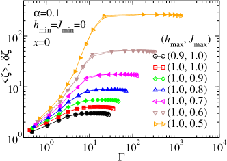
Figure 1: Renormalization-group flow of $\langle\zeta\rangle$ (open symbols) and $\delta\zeta$ (filled symbols) as a function of the cutoff energy scale, $\Gamma=\ln(\Omega_{I}/\Omega)$ for several different chains. Note that $\langle\zeta\rangle$ and $\delta\zeta$ agree to good approximation.

Without dissipation, the chain with $(h_{\rm max},J_{\rm max})=(0.9,1.0)$ would be in the ordered phase, the chain with (1.0,1.0) would be critical, and all others would be in the disordered phase. The figure shows that $\langle\zeta\rangle$ and $\delta\zeta$ initially increase under renormalization (corresponding to a rapid drop of the bond energies $J$); however after a sharp crossover, they settle on a constant value as expected from (14).

Figure 2 shows the corresponding data for the averages of the logarithmic field variable $\beta$, the cluster magnetic moment $\mu$, and their respective standard deviations.

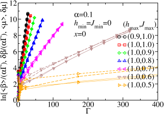
Figure 2: Renormalization-group flow of $\langle\beta\rangle$, $\langle\mu\rangle$ (open symbols) and $\delta\beta$, $\delta\mu$ (filled symbols) as a function of the cutoff energy scale, $\Gamma=\ln(\Omega_{I}/\Omega)$. The solid lines represent $\langle\beta\rangle$ and $\delta\beta$ while the dashed lines represent $\langle\mu\rangle$ and $\delta\mu$. Again, averages and standard deviations agree very well for $\Gamma\to\infty$.

They are plotted as $\ln(\langle\beta\rangle/(\alpha\Gamma))$, $\ln(\langle\mu\rangle)$, $\ln(\delta\beta/(\alpha\Gamma))$, and $\ln(\delta\mu)$ versus $\Gamma$. In this plot, the fixed-point forms (15), (16) correspond to straight lines. The figure shows that all data indeed follow the expected behavior after some short initial transients.

So far, we have analyzed the renormalization-group flow of the averages and standard deviations of the bond and field variables as well as the magnetic moments. For a full confirmation of the theoretical predictions (10) and (11), we need to analyze the full probability distributions. Figure 3 shows snapshots of the probability distributions $\mathcal{P}(\zeta)$, $\mathcal{R}_{\theta}(\theta)$ and $\mathcal{R_{\nu}}(\nu)$ along the renormalization-group flow.

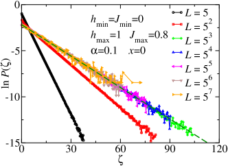
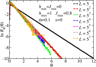
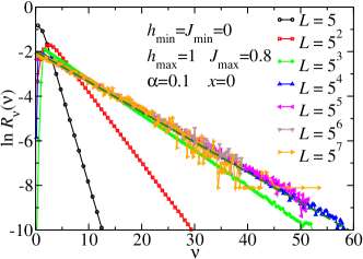
Figure 3: Probability distributions $\mathcal{P}(\zeta)$, $\mathcal{R}_{\theta}(\theta)$ and $\mathcal{R_{\nu}}(\nu)$ taken at different stages of the renormalization-group flow parametrized by the average distance $L$ of the remaining spin clusters. The dashed lines represent the fixed-point distributions (10) and (11). $(h_{\rm max},J_{\rm max})=(1.0,0.8)$, the parameters are as in Fig. 1 and 2.

Here, we have used the rescaled field variable $\theta=\beta/(\Gamma e^{\mathcal{P}_{0}\Gamma})$ and the rescaled moment $\nu=\mu/(\Gamma e^{\mathcal{P}_{0}})$. The figure shows that all distributions quickly approach the predicted functional forms. In the late renormalization-group stages, the numerical data are in excellent quantitative agreement with the theoretical results (10) and (11).

After having analyzed the behavior at fixed value of the dissipation strength $\alpha$, we now turn to the $\alpha$-dependence of the renormalization-group flow. Figure 4 shows the evolution of $\langle\zeta\rangle$, $\langle\beta\rangle$, and $\langle\mu\rangle$ as well as their standard deviations for different $\alpha$.

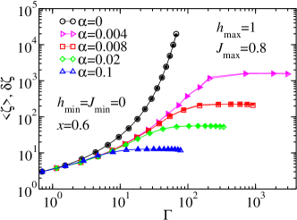
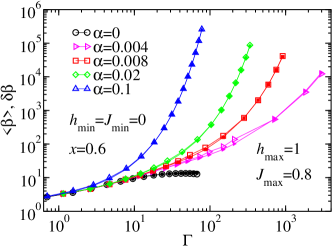
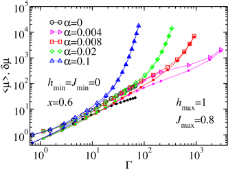
Figure 4: Renormalization-group flow of $\langle\zeta\rangle$, $\langle\beta\rangle$, and $\langle\mu\rangle$ (open symbols) as well as their standard deviations (filled symbols) as a function of the cutoff energy scale, $\Gamma=\ln(\Omega_{I}/\Omega)$ for $(h_{\rm max},J_{\rm max})=(1.0,0.8)$.

Because $h_{\rm max}=1.0$ is larger than $J_{\rm max}=0.8$, the dissipationless chain ($\alpha=0$) is in the disordered (Griffiths) phase. This can be seen from the rapid increase of the bond variable $\langle\zeta\rangle$, corresponding to a rapid drop of the interaction energies $J$ under renormalization while the field variable $\langle\beta\rangle$ approaches a constant and the moment $\langle\mu\rangle$ of the surviving clusters increases linearly with $\Gamma$ [4, 5].

In the presence of dissipation, the flow changes qualitatively when the typical cluster size reaches $1/\alpha$, as can be seen in the third panel of Fig. 4. Beyond this crossover scale, it is now the bond variable $\langle\zeta\rangle$ that saturates while the field variable $\langle\beta\rangle$ and the moment $\langle\mu\rangle$ rapidly increase, in agreement with Eqs. (14), (15), and (16). Thus, at a cluster moment of $1/\alpha$ the flow character changes from that of the disordered Griffiths phase to that of our inhomogeneously ordered phase. This crossover is caused by the fact that clusters with $\alpha\mu>1$ undergo the localization transition of the spin-boson problem [9] and are not decimated under further renormalization.

Finally, we have also studied the ultimate fate of the pseudo-critical point identified at intermediate scales by Schehr and Rieger. To this end, we have repeated the calculation of Ref. [12] for much longer chains of up to 16000 sites (averaging over 10⁶ disorder realizations). The quantity studied is the smallest excitation energy $\Delta$ of a finite chain, as estimated by the last nonzero transverse-field in the renormalization procedure. The upper panel of Fig. 5 shows the probability distribution of $\ln(\Omega_{I}/\Delta)$ for different chain sizes.

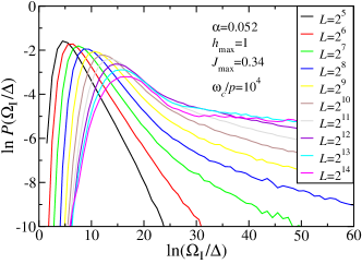
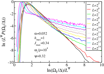
Figure 5: Probability distribution of the smallest energy gap $\Delta$ of a finite-size chain for different chain lengths. The parameters $h_{\rm max}=1.0$, $J_{\rm max}=0.34$, $h_{\rm min}=J_{\rm min}=0$, $x=0$, and $\alpha=0.052$ correspond to the pseudo-critical point of Ref. [12].

Following Ref. [12], only chains that are not yet frozen ($\Delta\neq 0$) at the end of the renormalization procedure are included in the distribution. The parameters $h_{\rm max}=1.0$, $J_{\rm max}=0.34$, $x=0$, and $\alpha=0.052$ exactly correspond to the pseudo-critical point of [12]. The figure shows that the character of the distribution changes significantly with increasing chain length $L$. The lower panel demonstrates that the data for $L\lessapprox 512$ and not too large $\ln(\Omega_{I}/\Delta)$ can be approximately scaled according to the pseudo-critical activated scaling form $\ln(\Omega_{I}/\Delta)\sim L^{\psi}$ with $\psi=0.32$. However, for longer chains the distributions do not scale. Instead, they become much broader, indicating a crossover to the functional form (11) characterizing the inhomogeneously ordered phase. Thus, the pseudo-critical behavior applies only to a transient regime of the renormalization-group flow and thus only to a transient energy or temperature window [13].

5 Conclusions

In summary, we have presented results of an extensive numerical strong-disorder renormalization group for the random transverse-field Ising model with Ohmic dissipation. Our simulations quantitatively confirm the analytical theory of Ref. [11]. Specifically, we have verified that the Ohmic dissipation destabilizes the quantum critical of the dissipationless system and the associated quantum Griffiths phase. No other critical point has been found. Instead, the low-energy behavior in the region of overlapping field and bond distributions is governed by a new line of fixed points describing the inhomogeneous tail of the ordered phase. Thus, the sharp quantum phase transition is destroyed by smearing due to the interplay of disorder and Ohmic dissipation. Note that Ohmic dissipation also suppresses the quantum Griffiths singularities at the percolation quantum phase transition [16] in a diluted transverse-field Ising model [17]. However, the percolation transition remains sharp because it is driven by the critical geometry of the lattice.

In addition to confirming the fixed-point structure of the analytical theory [11], our extensive numerical results also show that moderately disordered systems generically flow towards the new line of fixed points. The crossover to the asymptotic behavior occurs when the typical cluster moment reaches $1/\alpha$.

Let us conclude by putting our results into a broader perspective. Recently, a general classification has been put forward of phase transitions in the presence of weak disorder [8]. It is based on the effective dimensionality of the defects or rare regions. Three classes need to be distinguished. (i) If the defect dimension is below the lower critical dimension $d_{c}^{-}$ of the problem, the behavior is conventional; (ii) if it is right at $d_{c}^{-}$, the transition is of infinite-randomness type; and (iii) if it is above $d_{c}^{-}$, finite clusters can order independently leading to a smeared transition. In our case, individual rare regions can undergo the localization transition of the spin-boson problem [9]. The system therefore falls into the smeared-transition class.

The results for a dissipative Ising magnet must be contrasted with the behavior of systems with continuous O($N$) symmetry. While large Ising clusters freeze in the presence of Ohmic dissipation, O($N$) clusters continue to fluctuate with a rate exponentially small in their moment [18], putting the system into class (ii). This leads to a sharp transition controlled by an infinite-randomness critical point in the same universality class as the dissipationless random transverse-field Ising model [19, 20].

Our results directly apply to quantum phase transitions in disordered systems with discrete order parameter symmetry and Ohmic dissipation. The renormalization-group approach should be broadly applicable to a variety of disordered dissipative quantum systems such as arrays of resistively shunted Josephson junctions.

References

- [1] A.B. Harris, J. Phys. C 7 (1974) 1671.
- [2] R.B. Griffiths, Phys. Rev. Lett. 23 (1969) 17.
- [3] Y. Imry, Phys. Rev. B 15 (1977) 4448.
- [4] D.S. Fisher, Phys. Rev. Lett. 69 (1992) 534.
- [5] D.S. Fisher, Phys. Rev. B 51 (1995) 6411.
- [6] M. Thill and D.A. Huse, Physica A 214 (1995) 321.
- [7] A.P. Young and H. Rieger, Phys. Rev. B 53 (1996) 8486.
- [8] T. Vojta, J. Phys. A 39 (2006) R143.
- [9] A.J. Leggett et al., Rev. Mod. Phys. 59 (1987) 1.
- [10] T. Vojta, Phys. Rev. Lett. 90 (2003) 107202.
- [11] J.A. Hoyos and T. Vojta, Phys. Rev. Lett. 100 (2008) 240601.
- [12] G. Schehr and H. Rieger, Phys. Rev. Lett. 96 (2006) 227201.
- [13] G. Schehr and H. Rieger, J. Stat. Mech. (2008) P04012.
- [14] S.K. Ma, C. Dasgupta and C.K. Hu, Phys. Rev. Lett. 43 (1979) 1434.
- [15] C. Dasgupta and S.K. Ma, Phys. Rev. B 22 (1980) 1305.
- [16] T. Senthil and S. Sachdev, Phys. Rev. Lett. 77 (1996) 5292.
- [17] J.A. Hoyos and T. Vojta, Phys. Rev. B 74 (2006) 140401(R).
- [18] T. Vojta and J. Schmalian, Phys. Rev. B 72 (2005) 045438.
- [19] J.A. Hoyos, C. Kotabage and T. Vojta, Phys. Rev. Lett. 99 (2007) 230601.
- [20] T. Vojta, C. Kotabage and J.A. Hoyos, Phys. Rev. B 79 (2009) 024401.