Extinction of quasiparticle interference in underdoped cuprates with coexisting order

Abstract

Recent scanning tunnelling spectroscopy measurements [Y. Koksaka et al., Nature 454, 1072 (2008)] have shown that dispersing quasiparticle interference peaks in Fourier transformed conductance maps disappear as the bias voltage exceeds a certain threshold corresponding to the coincidence of the contour of constant quasiparticle energy with the antiferromagnetic zone boundary. Here we argue that this is caused by quasistatic short-range coexisting order present in the $d$-wave superconducting phase, and that the most likely origin of this order is disorder-induced incommensurate antiferromagnetism. We show explicitly how the peaks are extinguished in the related situation with coexisting long-range antiferromagnetic order, and discuss the connection with the realistic disordered case. Since it is the localized quasiparticle interference peaks rather than the underlying antinodal states themselves which are destroyed at a critical bias, our proposal resolves a conflict between scanning tunneling spectroscopy and photoemission regarding the nature of these states.

I Introduction

The understanding of how a Mott insulator with localized states becomes a metal as one gradually increases the carrier concentration remains one of the main challenges of condensed matter physics. This question may be intimately connected with the so-called nodal-antinodal dichotomy (sharp quasiparticles in the nodal region versus broad, gapped antinodal ”quasiparticles”) observed by angular resolved photoemission spectroscopy (ARPES) on underdoped cuprate materials.Damascelli03 ; FuLee06 Tunnelling spectroscopy has also been used to probe states in different regions of momentum space by the help of Fourier transform scanning tunneling spectroscopy (FT-STS).Hoffman1 ; Howald ; Hoffman2 ; vershinen ; mcelroy1 ; hashimoto In particular, it has been argued that the apparent incoherent antinodal states have their origin in the emergence of charge ordered regions in the underdoped regime.mcelroy1

In the $d$-wave superconducting (dSC) state near optimal doping, quasiparticle interference (QPI) observed by FT-STS is dominated by peaks at well-defined wavevectors ${\mathbf{q}}_{i}$ which agree well with those predicted by the so-called octet model.Hoffman1 ; mcelroy1 ; WangLee The contours of constant energy (CCE) of the Bogoliubov quasiparticle dispersion are generally shaped like curved ellipses (“bananas”) centered at the nodal points; seven different nonzero wavevectors ${\mathbf{q}}_{i}$ connect the tips of these bananas. The dispersion of the peaks at ${\mathbf{q}}_{i}$ allows one to extract the shape of the underlying Fermi surfaceSprunger as well as the momentum dependence of the superconducting energy gap.Hoffman1 A quantitative understanding of the amplitude and width of the peaks, however, is not straightforward to obtain, and depends rather sensitively on the nature of the scattering medium. A point-like scatterer, for example, in an otherwise homogeneous dSC leads to a landscape of some spot-like and some arc-like dispersive features close to ${\mathbf{q}}_{i}$ in the FT-STS imagesWangLee ; Tingfourier ; Franzold ; capriotti ; ZAH04 ; misra whereas experimental data appear mostly spot-like. Furthermore, the weights of the various peaks calculated in simple theories differ from experiment. There have been several theoretical attempts to remedy this situation by including more realistic models for the disorder present in Bi₂Sr₂CaCu₂O_8+δ (BSCCO). In particular, as realized recently, it appears important to include the gap inhomogeneity arising from the dopant atoms.mcelroyscience ; NAMH05 ; andersen06 ; nunner ; DellAnna ; ChengSu Models have also included the extended Coulomb potential arising in this material from partly screened Bi$\leftrightarrow$Sr substitutional disorder and the oxygen dopant atoms.nunner Nevertheless, a complete quantitative description of the FT-STS patterns is still lacking in the superconducting state.

FT-STS has also been used to probe the pseudogap state in the underdoped regime where non-dispersive (bias-independent) quasi-periodic conductance modulations has been identified both in BSCCOHowald ; vershinen ; mcelroy1 ; hashimoto ; liu and Ca_2-xNa_xCuO₂Cl₂ (Na-CCOC).hanaguri1 The origin of these peaks remains unknown at present but may be caused by short-range charge order, possibly connected to the existence of nested segments of the Fermi surface near the antinodal regions of the Brillouin zone.wise In BSCCO near optimal doping non-dispersive peaks have also been discussed in terms of pinned and disorder-induced charge order.sachdev ; chenyeh ; podolsky ; AHB03 ; linda In Na-CCOC it has been proposed that phonons play a crucial role in stabilizing a $d$-wave charge density wave order,DHLee or a surface transition to a commensurate charge density wave state.brown At present, however, it remains controversial whether true charge ordering is required for describing the non-dispersive LDOS modulations.ghosal ; chatterjee ; bascones

Recently, new developments in the FT-STS technique allowed for further detailed exploration of the electronic properties of underdoped Na-CCOC and BSCCO. For example, it was argued that tip-elevation errors can be avoided by studying the conductance-ratio $Z({\mathbf{r}},E=eV)=g({\mathbf{r}},V)/g({\mathbf{r}},-V)$ where $V$ is the bias voltage and $g$ the conductance, and the detailed properties of the LDOS modulations were investigated in this regime as well.hanaguri2 ; kohsaka ; hanaguri3 It was found that irrespective of the doping level, an ”extinction line” exists in momentum space, beyond which most of the dispersing FT-STS peaks (${\mathbf{q}}_{2}$,${\mathbf{q}}_{3}$,${\mathbf{q}}_{6}$,${\mathbf{q}}_{7}$) disappear, to be replaced by a reduced set (${\mathbf{q}}_{1}^{*}$,${\mathbf{q}}_{5}^{*}$) of roughly non-dispersive peaks.kohsaka This extinction line is doping independent and coincides at all doping levels with the antiferromagnetic (AF) zone boundary [lines joining the points $(0,\pm\pi)$ and $(\pm\pi,0)$]. At energies below the scale $\Delta_{0}$ where the CCE first touch the AF zone boundary, the FT-STS response is similar to the dispersing Bogoliubov quasiparticles obeying the octet model. At energies above $\Delta_{0}$, the response becomes highly spatially inhomogeneous and appears dominated by pseudogap excitations.

One popular picture of the nodal-antinodal dichotomy invokes intense scattering with momentum transfer near ($\pi,\pi$) which broadens states near the antinodal points. The problem with this picture in the superconducting state, however, is that the phase space for scattering is smallest at precisely these points of momentum space because the $d$-wave gap is largest there. Thus Graser et al.graserprb07 calculated the spin fluctuation spectrum within an RPA-type formalism and used it to determine the lifetime of states near the node and antinode of a dSC phase. This same framework produces a good description of the resonant magnetic response near ($\pi,\pi$) as measured by neutron scattering.eschrigreview Nevertheless their results, which were consistent with earlier work on quasiparticle lifetimes,Dahmetal1 ; Quinlan96 ; Dahmetal2 imply that inelastic scattering of the conventional itinerant spin-fluctuation type cannot severely broaden quasiparticle states in the superconducting state with momenta near the antinodes. This is of course consistent with ARPES experiments, which find broad but well-defined antinodal peaks in the superconducting state of BSCCO.Damascelli03 ; campuzano ; shi

One aspect of the physics of some underdoped cuprate materials which is left out of the conventional spin-fluctuation scattering analysis is the possibility of additional order coexisting with the dSC state at low temperatures. Static stripe order has been observed in several high-$T_{c}$ materials and appears especially pronounced near 1/8 doping;Tranquadareview in the La_2-xBa_xCuO₄ (LBCO) system, for example, charge order appears around 50K and persists to lower temperatures, where it coexists with spin order.fujita In addition, $\mu$SR has consistently reported so-called “cluster spin glass” (CSG) signatures of frozen magnetic order all over the underdoped cuprate phase diagram of La_2-xSr_xCuO₄ (LSCO) and BSCCO,julien ; panagopoulos generally attributed to disorder present in signficant amounts due to the way in which these materials are doped. In both LSCO and BSCCO, the nodal-antinodal dichotomy is also observed in ARPES measurements.xjzhou These observations suggest that quasiparticle scattering from short-range coexisting order might play an important role in explaining the extinction of the QPI peaks in the experiment by Kohsaka et al.kohsaka

There is no complete consensus on the origin of these ordering phenomena. One general notion is that disorder can pin fluctuating order while still reflecting the intrinsic correlations of the pure system.kivelson Whether the level of disorder present in these intrinsically disordered systems is too large to justify such an assumption is not clear. However, various concrete models of pinned fluctuating stripes have been proposedalvarez05 ; atkinson05 ; robertson ; delmaestro ; kaul ; andersen07 which resemble experiment in qualitative ways. An alternative starting point to understand the CSG phase assumes that dopants nucleate droplets of staggered order, which then interfere constructively to create quasi-long-range order.atkinson05 ; andersen07

These studies are related to the important question of whether AF correlations coexisting with preformed Cooper pairs are adequate to explain the pseudogap phase, or whether other types of ordering phenomena occur instead, or in addition.ZWang ; DHLee ; seo ; vojta08 Models of a disordered AF phase coexisting with $d$-wave pairs can reproduce a number of known experimental results: the magnetic correlations have been shown to protect the nodal quasiparticles;atkinson07 ; andersenkappa reproduce the Fermi arcs and nodal-antinodal dichotomy;alvarez08 as well as the temperature dependence of the superfluid densityatkinson07 and thermal conductivity.andersenkappa ; andersenDresden

Although the coexisting order in these systems is short-range, we know from neutron measurements in underdoped LSCOlake that correlation lengths can be quite long, of order 100 lattice spacings. It may therefore not be a bad starting point for the study of the effect of these correlations on QPI to assume a long-range ordered state. Here, we propose a concrete model for this effect by assuming the presence of a long-range AF state coexisting with superconductivity, and then investigating the consequences for the LDOS modulations. Even though the underdoped materials which exhibit magnetic ordering are characterized by incommensurate antiferromagnetism [with incommensurate peaks away from $(\pi,\pi)$], we assume $(\pi,\pi)$ ordering for simplicity. We focus on the origin of the extinction line, and not the high-energy LDOS modulations which require more realistic disorder models, possibly including charge ordering. In order to clearly elucidate the role of the AF order we consider for simplicity a single point-like scatterer. The results presented below should be important for understanding future FT-STS modelling using more realistic disorder configurations.

II Formalism

The FT-STS signal of a disordered dSC has been discussed rather extensively by theoretical models.WangLee ; Tingfourier ; Franzold ; capriotti ; ZAH04 ; misra In the present case of coexisting AF order, the translational symmetry is broken, and the formalism is very similar to the $d$-density wave approach discussed in e.g. Ref. bena, . The Hamiltonian reads

$$H = \sum_{{\mathbf{k}}\sigma}\left[\epsilon({\mathbf{k}})-\mu\right]c_{{\mathbf{k}}\sigma}^{\dagger}c_{{\mathbf{k}}\sigma}$$

$$+ \sum_{{\mathbf{k}}}\left[\sum_{\sigma}\sigma Mc_{{\mathbf{k+Q}}\sigma}^{\dagger}c_{{\mathbf{k}}\sigma}+\Delta({\mathbf{k}})c_{{\mathbf{k}}\uparrow}^{\dagger}c_{-{\mathbf{k}}\downarrow}^{\dagger}\right]+\mbox{H.c.},$$

where $c_{{\mathbf{k}}\sigma}^{\dagger}$ creates an electron with momentum ${\mathbf{k}}$ and spin $\sigma$, $M$ is the magnetization and ${\mathbf{Q}}=(\pi,\pi)$ is the AF ordering vector. We work in units where the lattice constant $a=1$. The superconducting $d$-wave gap function is $\Delta({\mathbf{k}})=\Delta\left(\cos k_{x}-\cos k_{y}\right)/2$, and the quasiparticle dispersion is $\epsilon({\mathbf{k}})=\epsilon_{1}({\mathbf{k}})+\epsilon_{2}({\mathbf{k}})$, where $\epsilon_{1}({\mathbf{k}})=-2t\left(\cos k_{x}+\cos k_{y}\right)$ and $\epsilon_{2}({\mathbf{k}})=-4t^{\prime}\cos k_{x}\cos k_{y}-2t^{\prime\prime}\left(\cos 2k_{x}+\cos 2k_{y}\right)$. It is convenient to split up the normal state band in this form due to the different symmetry properties of $\epsilon_{1}({\mathbf{k}})$ and $\epsilon_{2}({\mathbf{k}})$ with respect to momentum shifts of the AF ordering vector ${\mathbf{Q}}$; $\epsilon_{1}({\mathbf{k}}+{\mathbf{Q}})=-\epsilon_{1}({\mathbf{k}})$ and $\epsilon_{2}({\mathbf{k}}+{\mathbf{Q}})=\epsilon_{2}({\mathbf{k}})$. In terms of the following generalized Nambu spinor $\psi_{\mathbf{k}}^{\dagger}=\{c_{{\mathbf{k}}\uparrow}^{\dagger},c_{{\mathbf{k+Q}}\uparrow}^{\dagger},c_{-{\mathbf{k}}\downarrow},c_{{\mathbf{-k-Q}}\downarrow}\}$, we can write the Hamiltonian in the form

$$H=\sum_{\mathbf{k}}\psi_{\mathbf{k}}^{\dagger}A({\mathbf{k}})\psi_{\mathbf{k}},$$ (2)

where the sum is restricted to the reduced Brillouin zone (RBZ), $|k_{x}|+|k_{y}|\leq\pi$, and $A({\mathbf{k}})$ is given by

$$A({\mathbf{k}})=\left(\begin{array}[]{cccc}\epsilon_{1}({\mathbf{k}})+\epsilon_{2}({\mathbf{k}})-\mu&M&\Delta({\mathbf{k}})&0\\ M&-\epsilon_{1}({\mathbf{k}})+\epsilon_{2}({\mathbf{k}})-\mu&0&-\Delta({\mathbf{k}})\\ \Delta^{*}({\mathbf{k}})&0&-\epsilon_{1}({\mathbf{k}})-\epsilon_{2}({\mathbf{k}})+\mu&M\\ 0&-\Delta^{*}({\mathbf{k}})&M&\epsilon_{1}({\mathbf{k}})-\epsilon_{2}({\mathbf{k}})+\mu\end{array}\right).$$ (7)

The eigenvalues $\pm E_{1,2}({\mathbf{k}})$ of $A({\mathbf{k}})$ are given by

$$E_{1,2}({\mathbf{k}})=\sqrt{\left([\epsilon_{2}({\mathbf{k}})-\mu]\pm\sqrt{\epsilon_{1}^{2}({\mathbf{k}})+M^{2}}\right)^{2}+\Delta^{2}({\mathbf{k}})},$$ (8)

which for $\Delta({\mathbf{k}})=0$ reduces to $E_{M}^{\pm}({\mathbf{k}})=[\epsilon_{2}({\mathbf{k}})-\mu]\pm\sqrt{\epsilon_{1}^{2}({\mathbf{k}})+M^{2}}$, and for $M=0$ reduces to $E({\mathbf{k}})=\pm\sqrt{[\epsilon_{1}({\mathbf{k}})+\epsilon_{2}({\mathbf{k}})-\mu]^{2}+\Delta^{2}({\mathbf{k}})}$. The Greens function $G_{0}({\mathbf{k}},i\omega_{n})$ of the pure system is obtained from the equation

$$G_{0}({\mathbf{k}},i\omega_{n})^{-1}=i\omega_{n}I-A({\mathbf{k}}),$$ (9)

where $I$ denotes the $4\times 4$ identity matrix.

In the presence of an impurity term

$$H_{imp}=\sum_{{\mathbf{k}},{\mathbf{k}}^{\prime}\in RBZ}\psi_{\mathbf{k}}^{\dagger}V({\mathbf{k}},{\mathbf{k}}^{\prime})\psi_{{\mathbf{k}}^{\prime}},$$ (10)

the impurity-contribution to the full Greens function $G({\mathbf{k}},{\mathbf{k}}^{\prime},i\omega_{n})$ is given by

$$G({\mathbf{k}},{\mathbf{k}}^{\prime},i\omega_{n})=G_{0}({\mathbf{k}},i\omega_{n})T({\mathbf{k}},{\mathbf{k}}^{\prime},i\omega_{n})G_{0}({\mathbf{k}}^{\prime},i\omega_{n}),$$ (11)

where

$$T({\mathbf{k}},{\mathbf{k}}^{\prime},i\omega_{n})=V({\mathbf{k}},{\mathbf{k}}^{\prime})+$$ (12)

$$\sum_{{\mathbf{k}}^{\prime\prime}\in RBZ}V({\mathbf{k}},{\mathbf{k}}^{\prime\prime})G_{0}({\mathbf{k}}^{\prime\prime},i\omega_{n})T({\mathbf{k}}^{\prime\prime},{\mathbf{k}}^{\prime},i\omega_{n}).$$

For a point-like impurity $V({\mathbf{k}},{\mathbf{k}}^{\prime})$ [and $T({\mathbf{k}},{\mathbf{k}}^{\prime},i\omega_{n})$] become independent of ${\mathbf{k}}$ and ${\mathbf{k}}^{\prime}$. Specifically, a nonmagnetic $\delta$-function scatterer takes the form

$$V({\mathbf{k}},{\mathbf{k}}^{\prime})=V\left(\begin{array}[]{cccc}1&1&0&0\\ 1&1&0&0\\ 0&0&-1&-1\\ 0&0&-1&-1\end{array}\right).$$ (17)

The change in the LDOS from the pure phase $\delta N({\mathbf{q}},\omega)$, is given bybena

$$\delta N({\mathbf{q}},\omega) = \frac{i}{2\pi}\sum_{{\mathbf{k}}\in RBZ}g({\mathbf{k}},{\mathbf{q}},\omega),$$ (18)

where $g({\mathbf{k}},{\mathbf{q}},\omega)$ is defined as follows. Let ${\mathbf{k}}^{\prime}={\mathbf{k}}+{\mathbf{q}}$. If ${\mathbf{k}}^{\prime}$ is in the RBZ, then

$$g({\mathbf{k}},{\mathbf{q}},\omega)=\sum_{i=1}^{4}[G_{ii}({\mathbf{k}},{\mathbf{k}}^{\prime},s_{i}\omega)-G^{*}_{ii}({\mathbf{k}}^{\prime},{\mathbf{k}},s_{i}\omega)],$$ (19)

where $s_{i}=1$ for for the particle-hole sector $i=1,2$ and $s_{i}=-1$ for the hole-particle sector $i=3,4$. If ${\mathbf{k}}^{\prime}$ is not in the RBZ, let ${\mathbf{k}}^{\prime\prime}={\mathbf{k}}+{\mathbf{q}}-{\mathbf{Q}}$. For this case

$$g({\mathbf{k}},{\mathbf{q}},\omega) = \sum_{i=1,3}[G_{i,i+1}({\mathbf{k}},{\mathbf{k}}^{\prime\prime},s_{i}\omega)-G^{*}_{i,i+1}({\mathbf{k}}^{\prime\prime},{\mathbf{k}},s_{i}\omega)$$ (20)

$$+ G_{i+1,i}({\mathbf{k}},{\mathbf{k}}^{\prime\prime},s_{i}\omega)-G^{*}_{i+1,i}({\mathbf{k}}^{\prime\prime},{\mathbf{k}},s_{i}\omega)].$$

Here, $G({\mathbf{k}},{\mathbf{k}}^{\prime},\omega)$ is obtained by usual analytical continuation $i\omega_{n}\rightarrow\omega+i0^{+}$ of $G({\mathbf{k}},{\mathbf{k}}^{\prime},i\omega_{n})$. Below we introduce a finite lifetime broadening $\eta=0.02t$ such that $i\omega_{n}\rightarrow\omega+i\eta$, and the summation over the RBZ is performed using a $600\times 600$ mesh.

We use a band dispersion with $t=1.0,t^{\prime}=-0.3,t^{\prime\prime}=0.1$ and $\mu=-1.25$, which yields the normal state Fermi surface shown in Fig. 1. In addition, when studying the superconducting state we set $\Delta=0.6t$. In the following we focus the discussion on energies below this gap energy, which is taken unrealistically large for numerical purposes in order to highlight features at low energies. The impurity potential $V=0.1t$ is chosen to be weak in the sense that it does not produce any low-energy resonant states. For simplicity, we ignore any spatial structure of the local Wannier orbitals, rendering all results periodic in momentum space with respect to reciprocal lattice vectors.

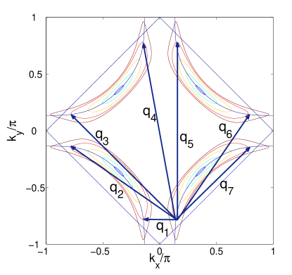
Figure 1: (Color online) (a) Contours of constant quasiparticle energy for the pure $d$-wave superconductor with $\Delta=0.6t$ at energies $\omega/t=0.0,0.075,0.225,0.375,0.5,0.57$. Also shown are the underlying normal state Fermi surface, the AF zone boundary, and the seven distinct nonzero wavevectors ${\bf q}_{i}$ connecting the banana tips.

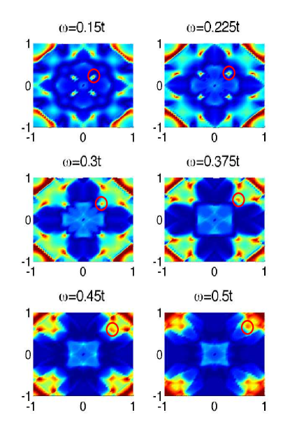
Figure 2: (Color online) QPI maps versus $q_{x}/\pi$ and $q_{y}/\pi$ in the dSC phase in the presence of single point-like potential scatterer of strength $V=0.1t$. Energies $\omega$ are as shown in the Figure titles. Some dispersing spot-like features corresponding to octet vectors ${\bf q}_{i}$ are easy to identify. For example, we have circled the ${\bf q}_{7}$ peak [see Fig. 1].

III Superconducting Phase

The QPI patterns in the pure dSC phase have been thoroughly discussed in the literature, and we will not dwell on them here. However, in order to discuss the effect of AF on the QPI, we show briefly some results for the pure dSC phase in this section. Figure 1 displays some typical CCE exhibiting the usual banana shaped form, and centered at the nodal points $(\pm 0.36,\pm 0.36)\pi$. The wavevectors ${\mathbf{q}}_{i}$ connecting the tips of these bananas, reveal where peaks in the FT-STS maps are expected, although matrix elements consisting of certain combinations of coherence factors are important for this simple picture to hold.WangLee ; Franzold Here we calculate the Fourier transform density of states $|\delta N|$ with $\delta N$ given by Eq.(18), and refer to it as a QPI map. Figure 2 shows QPI maps versus $q_{x}$ and $q_{y}$ at representative fixed energies inside the gap. For clarity, we have circled the ${\bf q}_{7}$ peak which is positioned along the (110) direction and disperses to higher momenta with increasing energy as expected from Fig. 1. Line cuts along the nodal and antinodal directions for the pure dSC phase are shown in Fig. 3 for both positive and negative energies, exhibiting clearly the dispersive QPI peaks discussed in the literature. The dispersion agrees well with the octet model,Hoffman1 which assumes that the scattering peaks are determined entirely by the wavevectors connecting each banana tip with all the others. It is easy to identify in Fig. 3 the octet peaks ${\bf q}_{3}$ and ${\bf q}_{7}$ in the (110) cut, and the ${\bf q}_{1}$ and ${\bf q}_{5}$ peaks in the (100) cut.

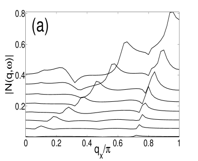
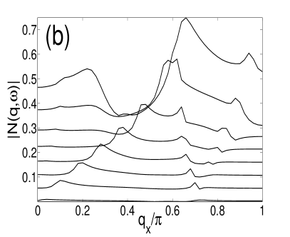
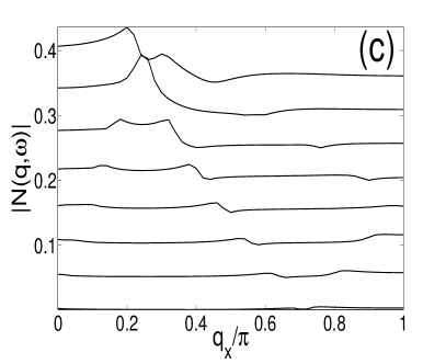
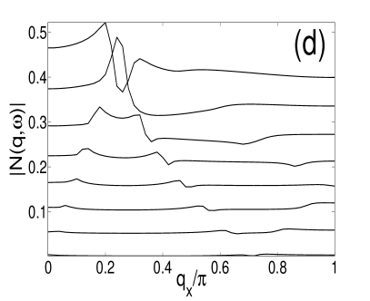
Figure 3: QPI line cuts along the (110) (a,b) and (100) (c,d) directions for the pure dSC phase. Panels (a,c) [(b,d)] correspond to positive [negative] energies at $|\omega|/t=0.01,0.075,0.15,0.225,0.3,0.375,0.45,0.5$ (bottom to top). For clarity the curves are displaced by 0.05.

IV Antiferromagnetic Phase

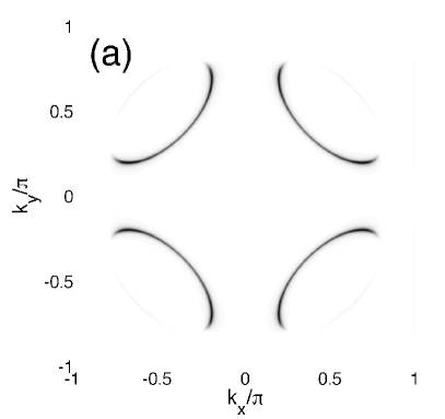
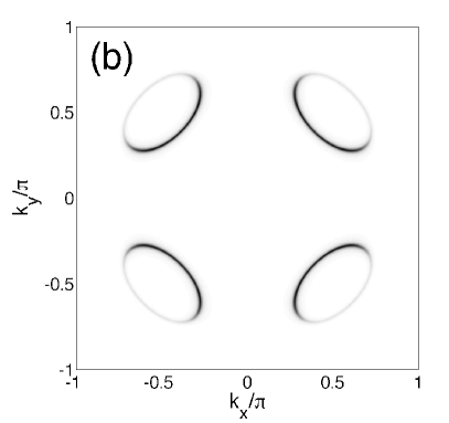
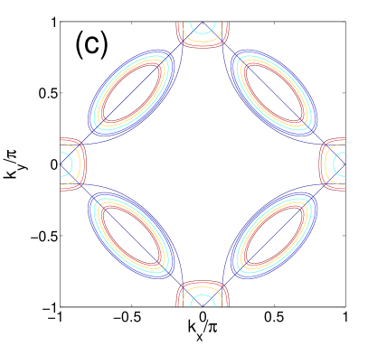
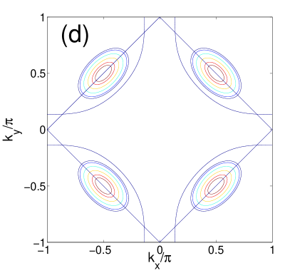
Figure 4: (Color online) Spectral weight $A({\mathbf{k}},\omega=0)$ in the pure AF phase with $M=0.5t$ (a), and $M=t$ (b). The lower two panels (c,d) show CCE at the same energies as in Fig. 1 for $M=0.5t$ (c), and $M=t$ (d).

In the pure dSC state, the spectral weight at the Fermi energy $A({\mathbf{k}},\omega=0)$ consists of four nodal points, which may be smeared slightly by disorder. On the other hand, in the pure metallic AF case, the spectral function can be written as

$$A({\mathbf{k}},\omega)=v^{2}({\mathbf{k}})\delta[\omega-E_{M}^{-}({\mathbf{k}})]+u^{2}({\mathbf{k}})\delta[\omega-E_{M}^{+}({\mathbf{k}})],$$ (21)

with $u^{2}({\mathbf{k}})=1/2[1+\epsilon_{1}({\mathbf{k}})/\sqrt{M^{2}+\epsilon_{1}^{2}({\mathbf{k}})}]$ and $v^{2}({\mathbf{k}})=1/2[1-\epsilon_{1}({\mathbf{k}})/\sqrt{M^{2}+\epsilon_{1}^{2}({\mathbf{k}})}]$. In Fig. 4(a,b) we show the spectral weight $A({\mathbf{k}},\omega=0)$ in a case with $M=0.5t$ (a) and $M=t$ (b). In both cases only the $E_{M}^{-}$ band crosses the Fermi level. As seen in Fig. 4(a,b), the outer ring of the Fermi pocket is washed out because of the $v^{2}({\mathbf{k}})$ coherence factor. This is caused by the unit cell doubling in the AF state, and a similar effect happens in e.g. the $d$-density wave scenario.chakravarty The checkerboard charge-order scenario for the pseudogap phase also reproduces a Fermi arc due to the difference in the coherence factors between the inner and outer parts of the arc.ZWang ; DHLee Disordered antiferromagnetism will further enhance this apparent spectral weight suppression on the outside of the pockets.singleton

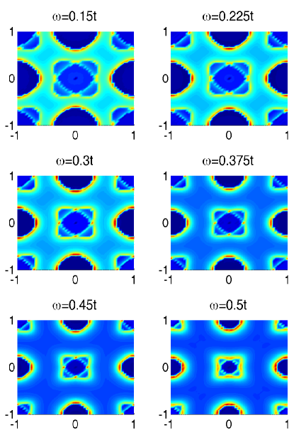
Figure 5: (Color online) Same as Fig. 2 but for the pure AF phase with $M=t$.

For the case with $M=t$ we show in Fig. 5 typical QPI maps in the pure AF phase. The QPI images are dominated by arcs of scattering intensity, rather than spots. The reason why distinct, isolated scattering wavevectors do not occur in the pure AF case is caused be the different coherence factors in this case. As discussed in Ref. Franzold, in the case of intra-nodal scattering, the origin of peaks in the QPI maps in the pure dSC phase is caused by the dSC coherence factors which conspire to significantly enhance the weight near the tips of the CCE resulting is a significant enhancement of the QPI response localized near ${\bf q}_{7}$. In the pure AF phase, on the other hand, the different coherence factors cause the weight to be evenly distributed along the CCE resulting in arc-like characteristic QPI features. We note that the momentum-resolved density of states, which is qualitatively similar (at least at negative energies) in the two phases, is not the cause of this qualitative difference in the QPI maps.

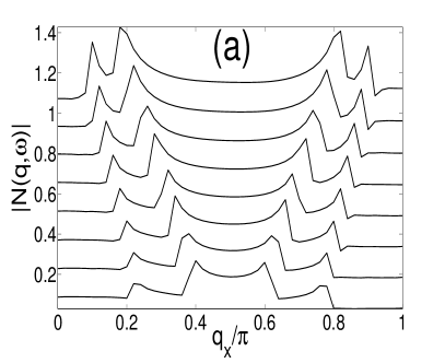
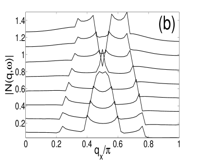
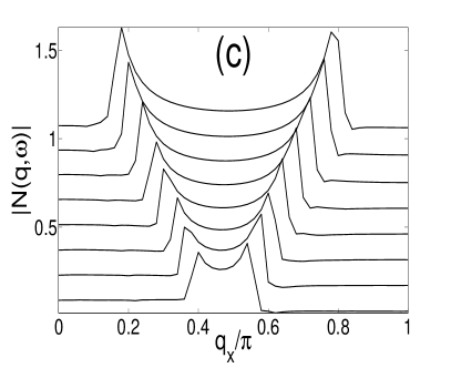
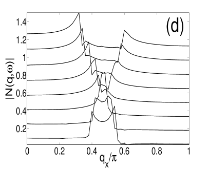
Figure 6: QPI line cuts along the (110) (a,b) and (100) (c,d) directions for the pure AF case with $M=t$. Panels (a,c) [(b,d)] correspond to positive [negative] energies at $|\omega|/t=0.01,0.075,0.15,0.225,0.3,0.375,0.45,0.5$ (bottom to top). For clarity the curves are displaced by 0.15.

In Fig. 6 we show line cuts along the nodal and antinodal directions at both positive and negative energies. We can understand the cusps in these line cuts from Fig. 4(d): consider for example the results presented in Fig. 6(a) showing cuts at positive energies along the (110) direction. The CCE clearly form ellipses centered around each nodal region as seen from Fig. 4(d). Scattering can be inter-ellipse or intra-ellipse, and leads to four cusps in agreement with Fig. 6(a). Since at positive energies the CCE shrink with increasing energy, the high momentum cusps resulting from inter-ellipse scattering move up with energy, and eventually merge. For the same reason, the low-momentum peaks resulting from intra-ellipse scattering disperse downwards with increasing energy. Since the negative energy CCE (not shown) expand with energy, we find the opposite dispersion in this case as seen from Fig. 6(b). From the cuts along the antinodal directions shown in Figs. 6(c,d), we see that the QPI response is actually strongest in this direction in agreement with the QPI maps in Fig. 5

Finally we note that in samples with inhomogeneous coexisting regions of dSC and AF, one way to determine whether which contribution of the QPI signal originates mainly from the dSC or the AF regions, is to compare the result to the bias reversed QPI map. In the pure dSC state the same positions of ${\mathbf{q}}$-spots should appear but with different weight, whereas in the AF phase the arcs in the QPI maps have also dispersed resulting in new locations of the cusps in e.g. the line cuts shown in Fig. 6. Below, we study the simpler case of a homogeneous coexisting phase of dSC and AF long-range order.

V Coexisting superconducting and antiferromagnetic phase

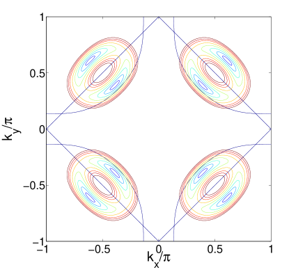
Figure 7: (Color online) Contours of constant energy for the coexisting phase with $\Delta=0.6t$ and $M=t$ plotted at energies $\omega/t=0.075,0.15,0.225,0.3,0.375,0.45,0.5,0.6$. The banana tips reach the AF zone boundary at $\omega=\Delta_{0}=0.33t$ when $M=t$.

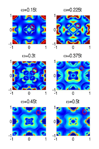
Figure 8: (Color online) QPI maps versus $q_{x}/\pi$ and $q_{y}/\pi$ in the coexisting AF and dSC phase in the presence of single point-like nonmagnetic impurity. Energies $\omega$ are as shown in the Figure titles. This figure can be directly compared to Fig. 2. Note the disappearance of the spot-like feature corresponding to octet vector ${\bf q}_{7}$ above the critical energy $\Delta_{0}=0.33t$.

In the homogeneous coexisting state (AF+dSC) with $\Delta,M\neq 0$, the $d$-wave gap collapses the arcs of spectral intensity at the Fermi level shown in Fig. 4(a,b) to nodal points. This robustness of the nodal points to antiferromagnetism away from half-filling follows directly from the fact that ($\pi,\pi$) does not nest the nodal points.eberg Some representative CCE for the coexisting phase are shown in Fig. 7. At low energies the CCE are again reminiscent of dispersing bananas, but now shifted off the normal state Fermi surface, and exist also in the shadow band outside the RBZ. This implies the existence of shadow banana tips and shadow QPI peaks, whose weight will however generally be suppressed due to coherence factors.

Once the banana tips reach the AF zone boundary, the CCE become similar to the pure AF case. In Fig. 8 we show the results of the QPI patterns in the coexisting phase. This figure can be directly compared to Fig. 2. We clearly see the mixing of the AF and dSC QPI features and the importance of the crossover scale set by the energy $\Delta_{0}$ where the CCE reach the AF zone boundary: at $\omega<\Delta_{0}$ ($\omega>\Delta_{0}$) the QPI is dominated by the pure dSC (AF) phase with the addition of possible shadow band features resulting from scattering involving the bananas outside the RBZ. Peaks generated by shadow bands are particularly evident in the QPI image at $\omega=0.225t$ in Fig. 8, and constitute a clear signature of the coexisting phase. For BSCCO, however, it seems likely that the disorder is simply too strong for these additional peaks to be observed [see next section]. In Fig. 8 we have circled the position of the ${\bf q}_{7}$ peak from the pure dSC phase [see also Fig. 2]. This peak appears to be extinguished when crossing the AF zone boundary at $\omega=\Delta_{0}$. For the band parameter and superconducting gap $\Delta=0.6t$ used in this paper, we have $\Delta_{0}=0.45t$ for $M=0.5t$, and $\Delta_{0}=0.33t$ for $M=t$.

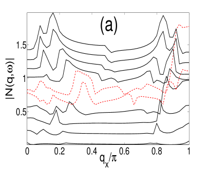
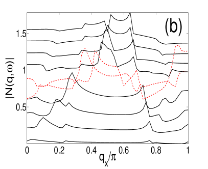
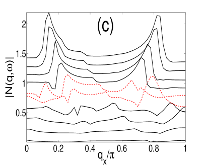
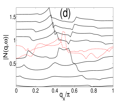
Figure 9: (Color online) QPI line cuts along the (110) (a,b) and (100) (c,d) directions for the pure coexisting AF and dSC phase with $M=t$ and $\Delta=0.6t$. Panels a,c (b,d) correspond to the following positive (negative) energies: $|\omega|/t=0.01,0.075,0.15,0.225,0.3,0.375,0.45,0.5,0.55,0.6$ (bottom to top). The line cuts close to the crossover region $\omega=\Delta_{0}$ are indicated by red dashed lines. For clarity the curves are displaced by 0.15.

Figure 9 shows the nodal and antinodal line cuts with the red dashed lines indicating the crossover region near $\Delta_{0}$. By comparison to Figs. 3 and 6, the resemblance to the dSC and AF state is again clear for $\omega<\Delta_{0}$ and $\omega>\Delta_{0}$, respectively. Note that despite the simplicity of the present model, it is evident from Figs. 8 and 9 that at $\omega>\Delta_{0}$ the FT-STS maps are dominated by slowly-dispersing peaks in the antinodal direction qualitatively similar to the experimental data.kohsaka These maxima disperse, however, more than those in Ref. kohsaka, and also appear to be more arclike than the experimentally observed ${\bf q}_{1}^{*}$ and ${\bf q_{5}^{*}}$ peaks. This may be because our simple model assumes a standard $d$-wave gap, whereas ARPES experiments reveal a gap which varies little near the antinodal points.kanigel We clearly also do not have in our model additional charge order leading to the nondispersive QPI peaks.

VI Effects of Disorder

So far the discussion has focussed on pure phases, dSC, AF, and AF+dSC in the presence of a single point-like nonmagnetic impurity. Clearly this situation is rather simplistic and should be extended to describe the QPI in a disordered short-range AF cluster glass phase as relevant for LSCO, and possibly also BSCCO. One way to model short-range AF correlations is by assuming that the AF ordering vector ${\mathbf{Q}}$ follows a Lorentzian probability distribution $p_{Q}$ peaked at $(\pi,\pi)$ and with a broadening given by $\xi_{AF}^{-1}$, the inverse of the AF correlation length. The main effects of disordering with such a distribution was studied in Ref. singleton, : only the part of the hole pockets which lie outside the RBZ is shifted. This means, for example, that scattering events involving the outer shadow band bananas [see Fig. 7] will be smeared out by this kind of disorder averaging, rendering the low-energy FT-STS patterns virtually identical to those of the pure dSC state. Nevertheless, modeling the disorder by a $p_{Q}$ distribution appears questionable for the CSG phase since it does not properly treat the spatial inhomogeneity of the spin glass, and misses e.g. additional low-energy states existing at the boundary regions between magnetic and superconducting domains.andersen05 Therefore, it would be interesting to compare with quasiparticle interference patterns from more realistic real-space disorder configurations similar to those produced in Refs. alvarez05, ; atkinson05, ; robertson, ; delmaestro, ; andersen07, ; andersenkappa, ; alvarez08, . The results presented in this paper should be helpful in providing an interpretation of results from future more realistic disorder modeling.

VII Conclusions

We have studied quasiparticle interference phenomena in a dSC phase with coexisting short-range AF order, as found, e.g. in the cluster spin glass phase of underdoped cuprates. To do so, we have assumed that much of the qualitative physics may be captured by studying the analogous problem with long-range AF order. In particular, we have calculated the QPI patterns arising from scattering from a single point-like impurity in the case of a pure metallic AF phase and a coexisting phase of both AF and dSC order. Due to different coherence factors in the AF and dSC phases, the QPI maps are dominated by peaks (arcs) in the dSC (AF) phase, respectively. In the case with coexisting order, low-energy quasiparticles propagate on contours which resemble the pure superconductor, so dispersive, localized interference spots similar to those predicted by the octet model for the pure dSC system are recovered. When the tips of these contours reach the AF zone face, however, the contours change abruptly to those characteristic of the pure AF, and the dispersing low-energy localized interference peaks are then extinguished, as reported by Kohsaka et al.kohsaka We expect that the remaining arc-like features at energies $\omega>\Delta_{0}$ are suppressed by the short-range nature of the true magnetic order in these systems.

The net result is a system where the low-energy quasiparticle interference features resemble those of the optimally doped superconducting samples, namely they disperse according to the octet model. For energies above the critical energy $\Delta_{0}$, these localized spot-like features in momentum space effectively disappear, as seen in experiment. Although the formation of AF long-range order itself may be viewed as a coherent multiple scattering process, we see from the study of the coexisting AF-dSC system that the quasiparticle states near the antinode are not destroyed by broadening in this process, but simply folded back. Thus in the realistic situation with short-range AF order, some scattering from AF modulations will occur, but still well-defined quasiparticle peaks should remain, as seen in ARPES. This resolves an apparent paradox in the comparison of the two experimental techniques in their view of the antinodal quasiparticles. It is the localized QPI ${\bf q}$-space structures due to these states which are destroyed, not the states themselves.

We emphasize that the formalism presented in this paper is essentially identical for any competing order scenario with ordering wavevector near $(\pi,\pi)$. We believe that the bulk of the experimental evidence support the identification of the competing phase with short-range incommensurate AF order or quasistatic fluctuations from incipient order, as observed in $\mu$SR. We have therefore discussed the extinction of QPI above a critical energy in this context, but other explanations with a similar structure may be possible.

In addition, we note that realistic simulations of the QPI patterns require a more sophisticated description of disorder than that adopted here. It is thought that the potential produced by a single defect has components in at least the screened Coulomb and pairing channels, and some account of the latter is known to be necessary to reproduce the correlations between dopant position and gap size observed in the BSCCO system.NAMH05 We have neglected these details here, but they are discussed e.g. in Ref. nunner, . Nevertheless, the patterns produced by our single potential scatterer were found to be sufficient to describe the basic phenomenology of Kohsaka et al.kohsaka for the octet ${\mathbf{q}}_{7}$ peak. It will be interesting to see if more sophisticated simulations can also reproduce the behavior of the other octet vectors and their weights correctly.

One aspect of the current picture which remains unclear is the extent to which static order is required. The QPI extinction phenomenon observed by Kohsaka et al.kohsaka is observed in BSCCO samples with doping levels 6-19%, i.e. including optimal doping where recent neutron experiments have claimed a 32 meV spin gap.fauque Still, near ($\pi,\pi$), some intensity remains below this energy, and $\mu$SR continues to indicate frozen magnetic order even in these samples at low temperatures.panagopoulos It may be that the magnetism in this system is simply too disordered to be seen by current neutron experiments. A more sophisticated treatment of short-range order is required to address these questions.

VIII Acknowledgement

The authors acknowledge valuable discussions with J. C. Davis, Z.-X. Shen, and M. Vojta. B. M. A. acknowledges support from the Villum Kann Rasmussen foundation, and P. J. H. from DOE-BES DE-FG02-05ER46236.

References

- (1) A. Damascelli, Z. Hussain, and Z.-X. Shen, Rev. Mod. Phys. 75, 473 (2003).
- (2) H. Fu. and D.-H. Lee, Phys. Rev. B 74, 174513 (2006).
- (3) J. E. Hoffman, K. McElroy, D.-H. Lee, K. M. Lang, H. Eisaki, S. Uchida, and J. C. Davis, Science 297, 1148 (2002).
- (4) C. Howald, H. Eisaki, N. Kaneko, M. Greven, and A. Kapitulnik, Phys. Rev. B 67, 014533 (2003).
- (5) K. McElroy, R. W. Simmonds, J. E. Hoffman, D.-H. Lee, J. Orenstein, H. Eisaki, S. Uchida, J. C. Davis, Nature (London) 422, 592 (2003).
- (6) M. Vershinin, S. Misra, S. Ono, Y. Abe, Y. Ando, and A. Yazdani, Science 303, 1995 (2004).
- (7) K. McElroy, D.-H. Lee, J. E. Hoffman, K. M. Lang, J. Lee, E. W. Hudson, H. Eisaki, S. Uchida, and J. C. Davis, Phys. Rev. Lett. 94, 197005 (2005).
- (8) A. Hashimoto, N. Momono, M. Oda, and M. Ido, Phys. Rev. B 74, 064508 (2006).
- (9) Q.-H. Wang and D.-H. Lee, Phys. Rev. B 67, 020511 (2003).
- (10) P. T. Sprunger, L. Petersen, E. W. Plummer, E. Lægsgaard, and F. Besenbacher, Science 275, 1764 (1997).
- (11) D. Zhang and C. S. Ting, Phys. Rev. B 67, 100506 (2003).
- (12) T. Pereg-Barnea and M. Franz, Phys. Rev. B 68, 180506 (2003).
- (13) L. Capriotti, D. J. Scalapino, and R. D. Sedgewick, Phys. Rev. B 68, 014508 (2003).
- (14) L.-Y. Zhu, W. A. Atkinson, and P. J. Hirschfeld, Phys. Rev. B 69, 060503 (2004).
- (15) S. Misra, M. Vershinen, P. Phillips, and A. Yazdani, Phys. Rev. B 70, 220503 (2004).
- (16) K. McElroy, J. Lee, J. A. Slezak, D.-H. Lee, H. Eisaki, S. Uchida, and J. C. Davis, Science 309, 1048 (2005).
- (17) T. S. Nunner, B. M. Andersen, A. Melikyan, and P. J. Hirschfeld, Phys. Rev. Lett. 95, 177003 (2005).
- (18) B. M. Andersen, A. Melikyan, T. S. Nunner, and P. J. Hirschfeld, Phys. Rev. B 74, 060501 (2006).
- (19) T. S. Nunner, W. Chen, B. M. Andersen, A. Melikyan, and P. J. Hirschfeld, Phys. Rev. B 73, 104511 (2006).
- (20) L. Dell’Anna, J. Lorenzana, M. Capone, C. Castellani, and M. Grilli, Phys. Rev. B 71, 064518 (2005).
- (21) M. Cheng and W. P. Su, Phys. Rev. B 72, 094512 (2005).
- (22) Y. H. Liu, K. Takeyama, T. Kurosawa, N. Momono, M. Oda, and M. Ido, Phys. Rev. B 75, 212507 (2007).
- (23) T. Hanaguri, C. Lupien, Y. Kohsaka, D.-H. Lee, M. Azuma, M. Takano, H. Takagi, and J. C. Davis, Nature (London) 430, 1001 (2004).
- (24) W. D. Wise, M. C. Boyer, K. Chatterjee, T. Kondo, T. Takeuchi, H. Ikuta, Y. Wang, and E. W. Hudson, Nature Phys. 4, 696 (2008).
- (25) A. Polkovnikov, M. Vojta, and S. Sachdev, Phys. Rev. B 65, 220509 (2002); Physics C 388-389, 19 (2003).
- (26) C.-T. Chen and N.-C. Yeh, Phys. Rev. B 68, 220505 (2003).
- (27) D. Podolsky, E. Demler, K. Damle, and B. I. Halperin, Phys. Rev. B 67, 094514 (2003).
- (28) B. M. Andersen, H. Bruus, and P. Hedegård, Phys. Rev. B 67, 134528 (2003).
- (29) L. Udby, B. M. Andersen, and P. Hedegård, Phys. Rev. B 73, 224510 (2006).
- (30) J.-X. Li, C.-Q. Wu, and D.-H. Lee, Phys. Rev. B 74, 184515 (2006).
- (31) S. E. Brown, E. Fradkin, and S. A. Kivelson, Phys. Rev. B 71, 224512 (2005).
- (32) A. Ghosal, A. Kopp, and S. Chakravarty, Phys. Rev. B 72, 220502 (2005).
- (33) U. Chatterjee, M. Shi, A. Kaminski, A. Kanigel, H. M. Fretwell, K. Terashima, T. Takahashi, S. Rosenkranz, Z. Z. Li, H. Raffy, A. Santander-Syro, K. Kadowaki, M. R. Norman, M. Randeria, and J. C. Campuzano, Phys. Rev. Lett. 96, 107006 (2006).
- (34) E. Bascones and B. Valenzuela, Phys. Rev. B 77, 024527 (2008).
- (35) T. Hanaguri, Y. Kohsaka, J. C. Davis, C. Lupien, I. Yamada, M. Azuma, M. Takano, K. Ohishi, M. Ono, and H. Takagi, Nature Phys. 3, 865 (2007).
- (36) Y. Kohsaka, C. Taylor, P. Wahl, A. Schmidt, J. Lee, K. Fujita, J. Alldredge, J. Lee, K. McElroy, H. Eisaki, S. Uchida, D.-H. Lee, and J. C. Davis, Nature (London) 454, 1072 (2008).
- (37) T. Hanaguri, Y. Kohsaka, M. Ono, M. Maltseva, P. Coleman, I. Yamada, M. Azuma, M. Takano, K. Ohishi, and H. Takagi (unpublished).
- (38) S. Graser, P. J. Hirschfeld, and D. J. Scalapino, Phys. Rev. B 77, 184504 (2008).
- (39) M. Eschrig, Adv. Phys. 55, 47 (2006).
- (40) T. Dahm and L. Tewordt, Phys. Rev. Lett. 74, 793 (1995).
- (41) S. Quinlan, P. J. Hirschfeld, and D. J. Scalapino, Phys. Rev. B 53, 8575 (1996).
- (42) T. Dahm, P. J. Hirschfeld, D. J. Scalapino, and L.-Y. Zhu, Phys. Rev. B 72, 214512 (2005).
- (43) J. C. Campuzano, H. Ding, M. R. Norman, H. M. Fretwell, M. Randeria, A. Kaminski, J. Mesot, T. Takeuchi, T. Sato, T. Yokoya, T. Takahashi, T. Mochiku, K. Kadowaki, P. Guptasarma, D. G. Hinks, Z. Konstantinovic, Z. Z. Li, and H. Raffy, Phys. Rev. Lett. 83, 3709 (1999).
- (44) M. Shi, A. Bendounan, E. Razzoli, S. Rosenkranz, M. R. Norman, J. C. Campuzano, J. Chang, M. Mansson, Y. Sassa, T. Claesson, O. Tjernberg, L. Patthey, N. Momono, M. Oda, M. Ido, S. Guerrero, C. Mudry, and J. Mesot, arXiv:0810.0292v1.
- (45) J. Tranquada in: Handbook of High Temperature Superconductivity: Theory and Experiment, editor J. R. Schrieffer, associate editor J. S. Brooks (Springer Verlag, Hamburg, 2007).
- (46) M. Fujita, H. Goka, K. Yamada, J. M. Tranquada, and L. P. Regnault, Phys. Rev. B 70, 104517 (2004).
- (47) M.-H. Julien, Physica B 329-333, 693 (2003).
- (48) C. Panagopoulos J. L. Tallon, B. D. Rainford, J. R. Cooper, C. A Scott, and T. Xiang, Solid State Comm. 126, 47 (2003).
- (49) X. J. Zhou, T. Yoshida, D.-H. Lee, W. L. Yang, V. Brouet, F. Zhou, W. X. Ti, J. W. Xiong, Z. X. Zhao, T. Sasagawa, T. Kakeshita, H. Eisaki, S. Uchida, A. Fujimori, Z. Hussain, and Z.-X. Shen, Phys. Rev. Lett. 92, 187001 (2004).
- (50) S. A. Kivelson, I. P. Bindloss, E. Fradkin, V. Oganesyan, J. M. Tranquada, A. Kapitulnik, and C. Howald, Rev. Mod. Phys. 75, 1201 (2003).
- (51) G. Alvarez, M. Mayr, A. Moreo, and E. Dagotto, Phys. Rev. B 71, 014514 (2005); M. Mayr, G. Alvarez, A. Moreo, and E. Dagotto, Phys. Rev. B 73, 014509 (2006).
- (52) W. A. Atkinson, Phys. Rev. B 71, 024516 (2005).
- (53) J. A. Robertson, S. A. Kivelson, E. Fradkin, A. C. Fang, and A. Kapitulnik, Phys. Rev. B 74, 134507 (2006).
- (54) A. Del Maestro, B. Rosenow, and S. Sachdev, Phys. Rev. B 74, 024520 (2006).
- (55) M. Vojta, T. Vojta, and R. K. Kaul, Phys. Rev. Lett. 97, 097001 (2006).
- (56) B. M. Andersen, P. J. Hirschfeld, A. P. Kampf, and M. Schmid, Phys. Rev. Lett. 99, 147002 (2007).
- (57) C. Li, S. Zhou, and Z. Wang, Phys. Rev. B 73, 060501 (2006).
- (58) K. Seo, H.-D. Chen, and J. Hu, Phys. Rev. B 76, 020511 (2007); Phys. Rev. B 78, 094510 (2008).
- (59) M. Vojta and O. Rösch, Phys. Rev. B 77, 094504 (2008).
- (60) W. A. Atkinson, Phys. Rev. B 75, 024510 (2007).
- (61) B. M. Andersen and P. J. Hirschfeld, Phys. Rev. Lett. 100, 257003 (2008).
- (62) G. Alvarez and E. Dagotto, Phys. Rev. Lett. 101, 177001 (2008).
- (63) B. M. Andersen and P. J. Hirschfeld, Physica (Amsterdam) 460C, 744 (2007).
- (64) B. Lake, H. M. Rønnow, N. B. Christensen, G. Aeppli, K. Lefmann, D. F. McMorrow, P. Vorderwisch, P. Smeibidl, N. Mangkorntong, T. Sasagawa, M. Nohara, H. Takagi, and T. E. Mason, Nature (London) 415, 299 (2002).
- (65) C. Bena, S. Chakravarty, J. Hu, and C. Nayak, Phys. Rev. B 69, 134517 (2004).
- (66) S. Chakravarty, C. Nayak, and S. Tewari, Phys. Rev. B 68, 100504 (2003).
- (67) N. Harrison, R. D. McDonald, and J. Singleton, Phys. Rev. Lett. 99, 206406 (2007).
- (68) E. Berg, C.-C. Chen, and S. A. Kivelson, Phys. Rev. Lett. 100, 027003 (2008).
- (69) A. Kanigel, M. R. Norman, M. Randeria, U. Chatterjee, S. Souma, A. Kaminski, H. M. Fretwell, S. Rosenkranz, M. Shi, T. Sato, T. Takahashi, Z. Z. Li, H. Raffy, K. Kadowaki, D. Hinks, L. Ozyuzer, and J. C. Campuzano, Nature Phys. 2, 447 (2006).
- (70) B. M. Andersen, I. V. Bobkova, P. J. Hirschfeld, and Yu. S. Barash, Phys. Rev. B 72, 184510 (2005).
- (71) B. Fauqué, Y. Sidis, L. Capogna, A. Ivanov, K. Hradil, C. Ulrich, A.I. Rykov, B. Keimer, and P. Bourges, Phys. Rev. B 76, 214512 (2007).