Dependence of Interstellar Turbulent Pressure on Supernova Rate

Abstract

Feedback from massive stars is one of the least understood aspects of galaxy formation. We perform a suite of vertically stratified local interstellar medium (ISM) models in which supernova rates and vertical gas column densities are systematically varied based on the Schmidt-Kennicutt law. Our simulations have a sufficiently high spatial resolution (1.95 pc) to follow the hydrodynamic interactions among multiple supernovae that structure the interstellar medium. At a given supernova rate, we find that the mean mass-weighted sound speed and velocity dispersion decrease as the inverse square root of gas density. The sum of thermal and turbulent pressures is nearly constant in the midplane, so the effective equation of state is isobaric. In contrast, across our four models having supernova rates that range from one to 512 times the Galactic supernova rate, the mass-weighted velocity dispersion remains in the range 4–6 km s^-1. Hence, gas averaged over $\sim$100 pc regions follows $P\propto\rho^{\,\alpha}$ with $\alpha\approx 1$, indicating that the effective equation of state on this scale is close to isothermal. Simulated H I emission lines have widths of 10–18 km s^-1, comparable to observed values. In our highest supernova rate model, superbubble blow-outs occur, and the turbulent pressure on large scales is $\gtrsim$4 times higher than the thermal pressure. We find a tight correlation between the thermal and turbulent pressures averaged over $\sim$100 pc regions in the midplane of each model, as well as across the four ISM models. We construct a subgrid model for turbulent pressure based on analytic arguments and explicitly calibrate it against our stratified ISM simulations. The subgrid model provides a simple yet physically motivated way to include supernova feedback in cosmological simulations.

1. Introduction

The observed vertical distribution of gas in the Galaxy, especially the cold neutral H I component at large heights, cannot be supported by thermal pressure alone (Lockman & Gehman 1991; Ferrara 1993). Often invoked to provide the required additional pressure are turbulent motions of the interstellar gas, magnetic fields, and cosmic rays (Boulares & Cox 1990; Lockman & Gehman 1991). Of these, turbulent pressure is perhaps the dominant pressure component in the interstellar medium (ISM; McKee 1990). There are strong reasons to believe that supersonic turbulence also regulates star formation processes in molecular clouds by lowering the efficiency of star formation (Elmegreen & Scalo 2004; Mac Low & Klessen 2004; Krumholz & McKee 2005; Krumholz & Tan 2007).

Supernova (SN) explosions are thought to be the dominant agent for producing turbulent motions in star-forming parts of galaxies (Norman & Ferrara 1996; Mac Low & Klessen 2004). Interactions between blast waves from multiple SNe lead to compression and shearing of the gas. In extreme cases, explosions that are spatially and temporally correlated may collectively generate a superwind, observed at both low (e.g., Martin 1999; Heckman et al. 2000) and high redshifts (Pettini et al. 2001, 2002; Shapley et al. 2003; Weiner et al. 2008). McKee & Ostriker (1977) provided a picture of the ISM in which three distinct phases regulated by SN explosions exist in rough pressure equilibrium. The multiphase model does not directly include turbulent pressure produced by interactions among multiple SN-driven blast waves and large pressure fluctuations in the ISM. Numerical simulations (Rosen & Bregman 1995; Korpi et al. 1999; Gazol-Patiño & Passot 1999; de Avillez & Berry 2001; Kim 2004; de Avillez & Breitschwerdt 2004, 2005; Mac Low et al. 2005; Slyz et al. 2005; Joung & Mac Low 2006, hereafter Paper I; Tasker & Bryan 2006) and observations of thermally unstable gas (Heiles 2001; Heiles & Troland 2003, 2005) also support this dynamic picture. Since turbulent pressure is a significant, sometimes the dominant, form of pressure in the ISM, its inclusion is vital for any realistic model of the ISM.

Another motivation for this study comes from longstanding problems in cosmology. The standard cold dark matter paradigm has been widely successful in explaining structures on cosmological scales (Cen et al. 1994; Zhang et al. 1995; Rauch 1998; Bertschinger 1998; Cen & Ostriker 2000; Springel et al. 2005; Dunkley et al. 2008). Yet our understanding of the luminous matter on galactic scales remains seriously incomplete, mainly due to complexities of baryon physics, for which additional nonlinear thermal and hydrodynamic processes must be taken into account. A prime example is the galaxy luminosity function, which shows lower abundances of galaxies both on the faint and the bright ends compared to the halo mass distribution (e.g., Benson et al. 2003). Other outstanding astrophysical problems include incorrect predictions for the size of disk galaxies (the “angular momemtum problem”; e.g., Navarro & White 1994; Steinmetz & Navarro 1999) and for the fraction of gas that should have cooled to form galaxies (the “overcooling problem”).

Feedback from massive stars and active galactic nuclei plays a central role to explain these discrepancies in recent semi-analytic models (Croton et al. 2006; Bower et al. 2006; Hopkins et al. 2008; Somerville et al. 2008). Despite mounting evidence that SNe played a major role in galaxy formation (see, e.g., Adelberger et al. 2003 and references therein), it has been difficult to incorporate the details of stellar feedback into cosmological simulations. Early studies found that thermal energy input did not affect the ISM significantly, as it was radiated away almost instantly (Katz 1992; Navarro & White 1993). This was due to a lack of numerical resolution, which led to an absence of hot gas that would have radiated inefficiently and substantially decreased the overall cooling rate. Past attempts to resolve this difficulty (e.g., Kauffman et al. 1993; Somerville & Primack 1999; Efstathiou 2000; Thacker & Couchman 2001; Springel & Hernquist 2003) have been phenomenological in nature, as they contain one or more free parameters that need to be adjusted to match observations, e.g., the observed rates of star formation. What is lacking is a detailed high-resolution 3D model of turbulent flows within a small region of the ISM, to help identify basic properties of interstellar turbulence.

Our aim in this paper is to provide a framework in which to handle SN feedback in cosmological simulations. We divide this challenging task into two parts. First, we run a suite of numerical simulations of stratified ISM driven by discrete SN explosions. The SN rate and the vertical gas column density are systematically varied over wide ranges to examine how the velocity dispersion changes as a function of the gas density, length scale, and the assumed SN rate. In particular, we study the distribution and variation of turbulent pressure in these models. These local, high-resolution simulations have high enough spatial resolution to follow turbulent motions of the interstellar gas in detail.

The second step is to use the local ISM models to find a prescription for the physics unresolved in global, cosmological simulations so that we have a better idea of how to handle SN feedback. We propose a subgrid model based on heuristic analytic arguments and simulation results. The idea is as follows: If we average relevant physical quantities over scales greater than the largest energy containing scale, we may describe the large-scale dynamics of the ISM that is insensitive to the details of the small-scale physics. This is motivated by similar studies in the past (Yepes et al. 1997; Springel 2000) as well as the new finding in Paper I that $>$90% of the total kinetic energy of the disk is contained on scales below 200 pc, comparable to the size of resolution elements in current cosmological simulations (e.g., Governato et al. 2004, 2007; Cen et al. 2005; Naab et al. 2007; Gibson et al. 2008; Joung et al. 2008). This suggests the interesting possibility that the SN-driven turbulence may be handled separately as subgrid physics in those simulations. Based on the physical characteristics of our local ISM models with discrete SN explosions, the subgrid model is physically well-motivated. We apply the results of our ISM models by formulating an accurate feedback prescription after deriving an effective equation of state for turbulent pressure of the medium. Such a prescription may be used to examine the effect of SN feedback in large cosmological volumes.

Dib et al. (2006) investigated the relationship between the velocity dispersion of the gas and the SN rate in 3D simulations of unstratified, periodic boxes with a fixed mean density. Their aim was to explore the observed constancy of the velocity dispersion in the outer parts of galactic disks (Dickey et al. 1990; Kamphuis 1993) and the transition to the starburst regime. They simulated a (1 kpc)³ volume of the unstratified ISM with 128³ cells for various SN rates, while keeping the gas density of the box constant. They found nearly constant velocity dispersions for the H I gas at relatively low SN rates (0.01 to 0.5 times the Galactic value; note thtat they took a Galactic SN rate per volume of $2.58\times 10^{2}$ Myr^-1 kpc^-3), as well as a transition to the starburst regime at about the star formation rate per unit area of 0.5–1$\times$10^-2 M_⊙ kpc^-2 yr^-1 (assuming a Salpeter initial mass function; Salpeter 1955), in good agreement with observations. The present study extends their work to stratified atmospheres at higher spatial resolution where the gas density is systematically increased with increasing SN rate.

The basic features of our ISM models are described in § 2. In § 3, we describe the thermal and structural properties of the models. We demonstrate in § 4 that the turbulent pressure of a medium with a given SN rate is independent of the local density, and study how the velocity dispersion and H I linewidth vary as a function of the assumed SN rate. Using these results, we construct a new subgrid model and calibrate it against the ISM simulations in § 5. Finally, we discuss several outstanding open issues (§ 6) and summarize our main results (§ 7).

2. Local ISM Simulations

We use the model described in Paper I and its extensions described here. Our simulations are performed using Flash v2.4, an Eulerian astrophysical hydrodynamics code with adaptive mesh refinement (AMR) capability, developed by the Flash Center at the University of Chicago (Fryxell et al. 2000). It solves the Euler equations using the piecewise-parabolic method (Colella & Woodward 1984) to handle compressible flows with shocks. For parallelization, the Message-Passing Interface library is used; the AMR is handled by the PARAMESH library.

Although, in the present work, we consider SNe as the only source of interstellar turbulence, other processes such as gravitational instability (e.g., Li et al. 2005a), magneto-Jeans instability (Kim & Ostriker 2002), magnetorotational instability (e.g., Piontek & Ostriker 2005), expanding H II regions (Matzner 2002) and protostellar outflows (Haverkorn et al. 2004; Nakamura & Li 2007; Banerjee et al. 2007; Carroll et al. 2008) should all contribute to the observed turbulence on various length scales. However, Mac Low & Klessen (2004) argue that these other processes may play relatively minor roles. We assume that they are insignificant on the spatial scales resolved in our models.

Our computation box contains a volume of (0.5 kpc)${}^{2}\times$(10 kpc), elongated in the vertical direction. If the grid were fully resolved at our maximum resolution of 1.95 pc, it would contain 256${}^{2}\times$5120 zones, but fully refined cells are mostly concentrated near the galactic midplane (the central $\pm 200$ pc) of our models. The gravitational potential of Kuijken & Gilmore (1989) is employed. For simplicity, the gravitational potential is fixed for all models, except in the model with the highest SN rate (512x), where the increased gas surface density dominates the gravitational potential, as it exceeds the assumed stellar mass surface density of $4.46\times 10^{7}$ M_⊙ kpc^-2 (Binney & Tremaine 1987). Assuming the Schmidt-Kennicutt law and taking $\Sigma_{\rm tot}=75$ M_⊙ pc^-2 and $\Sigma_{\rm gas}=5.3$ M_⊙ pc^-2 for the solar neighborhood (Binney & Tremaine 1987), we increase the gravitational acceleration due to the disk component in the Kuijken & Gilmore potential by a factor of 11 for the 512x model. This is our standard 512x model, and the results are based on this model, unless otherwise noted. For comparison, we also ran a model with the same SN rate but with the gravitational potential used in the lower SN rate models; this latter model will be denoted 512xL. Self-gravity of gas is not included. Outflow boundary conditions are used in the upper and lower surfaces parallel to the Galactic plane, while periodic boundary conditions are employed elsewhere.

For each SN explosion, we dump thermal energy $E_{\rm SN}=10^{51}$ ergs in a small sphere whose radius varies as a function of the local density. The radii are chosen such that radiative losses inside the spheres are negligible in the first few timesteps after explosions (Paper I); they usually range between $\sim$7 and $\sim$50 pc. We use them to trace the thermal history of metal particles and to estimate their escape fraction from the galaxy. We assume that a fixed fraction, 3/5, of the Type II SNe are closely correlated in space and in time as a way of simulating superbubbles. The remaining explosions have random positions scattered through the galaxy mass, with scale heights of 325 pc for Type I and 90 pc for Type II SNe, to represent field SNe. The minimum number of SNe $n_{\rm sn,min}=7$, while the average and maximum numbers of SNe per superbubble $\langle n_{\rm sn}\rangle$ and $n_{\rm sn,max}$ are determined by a power-law distribution $dN_{\rm B}\propto n_{*}^{2}\,dn_{*}$ yielding the values given in Table 1 (Kennicutt et al. 1988; see also Paper I for details). We fix the Type I SN rate at the Galactic value $\Sigma_{\rm*,I}=6.58$ Myr^-1 kpc^-2 in all models, as they take $>$1 Gyr to explode.

Table 1Parameters for the ISM simulations

model	$\dot{\Sigma}_{\rm*,II}$ a	$\Sigma_{\rm gas}$ b	$\Gamma$ c	$n_{\rm sn,max}$	$\langle n_{\rm sn}\rangle$
1x	11.0, 16.4	1.87(6)	8.50(-26)	40	14.8
8x	98.0, 147.	8.23(6)	1.55(-25)	320	27.4
64x	794., 1190.	3.63(7)	2.78(-25)	2560	41.4
512x	6360., 9540.	1.61(8)	5.11(-25)	20480	55.9

Note. — The SN rates per unit area are in units of Myr^-1 kpc^-2. Exponents are given parenthetically.

We run a suite of numerical models with wide ranges of SN rates and gas column densities, as listed in Table 1. We adopt SN rates per unit area, $\dot{\Sigma}_{*}$, of 1, 8, 64, and 512 times the Galactic rate (see Table 1 for the exact values adopted), and vary the gas column densities systematically following the Schmidt-Kennicutt law (Kennicutt 1998). Wong & Blitz (2002) reported observational evidence for seven CO-bright spiral galaxies that the azimuthally averaged star formation rate per unit area scales with the gas column density similarly to the disk-averaged star formation law (see Li et al. 2006 for similar results from numerical simulations). More recently, Kennicutt et al. (2007) reported evidence that the same star formation law is satisfied on scales of 0.5–2 kpc. The initial gas column densities $\Sigma_{\rm gas}$ are determined by inverting the relation

$$\dot{\Sigma}_{*}=A\,\left(\frac{\Sigma_{\rm gas}}{1\;{\rm M}_{\odot}\;{\rm pc}^{-2}}\right)^{1.4}\,.$$ (1)

where the coeffcient $A=2.5\times 10^{-4}\;{\rm M}_{\odot}\;{\rm yr}^{-1}\;{\rm kpc}^{-2}$. As the Schmidt-Kennicutt law holds in various physical conditions found in galaxies, we believe that our choices of ($\Sigma_{\rm gas}$, $\dot{\Sigma}_{*}$) are representative of typical regions in actual galaxies.

Radiative cooling appropriate for an optically thin plasma with $Z$$=$$Z_{\odot}$ (Dalgarno & McCray 1972; Sutherland & Dopita 1993; see Fig. 1 of Paper I) and a diffuse heating term that accounts for the photoelectric heating (Wolfire et al. 1995, 2003) of the neutral gas are also included. The diffuse heating rate $\Gamma$ in each model may not be directly proportional to $\dot{\Sigma}_{*}$ because the far-ultraviolet (FUV) radiation responsible for the photoelectric heating ($h\nu=6$–$13$ eV) may be significantly shielded in regions of high densities. In reality, the FUV radiation field is spatially nonuniform and time-varying (Parravano et al. 2003). However, as radiative transfer is not included in our calculations, we resort to a simple scaling relation. To compute the mean intensity of the FUV radiation appropriate for each ISM model, we imagine a medium that emits and absorbs radiation uniformly. In the optically thick limit (appropriate for our box size of 500 pc), the intensity of the FUV radiation, $I_{\rm FUV}=j_{\nu}/\alpha_{\nu}\,$, where $j_{\nu}$ is the emissivity and $\alpha_{\nu}=n\sigma$ is the absorption coefficient with the number density of absorbers, $n$, and their cross-section, $\sigma$. Assuming $j_{\nu}\propto\dot{\Sigma}_{*}\propto\Sigma_{\rm gas}^{\,1.4}\,$ and $n\propto\Sigma_{\rm gas}$ (since the gas scale height $H_{\rm gas}$ is only weakly dependent on the SN rate, as shown later), we obtain $I_{\rm FUV}\propto\Sigma_{\rm gas}^{\,0.4}\propto\dot{\Sigma}_{*}^{\,2/7}$. With the additional assumption that $\Gamma$ is proportional to the intensity of the FUV radiation, we obtain $\Gamma\propto\dot{\Sigma}_{*}^{2/7}$. As in Paper I, the diffuse heating rate in each model declines exponentially away from the galactic midplane with a scale height of 300 pc.

We note that another set of models was run with a different scaling relation for the diffuse heating rate: $\Gamma\propto\dot{\Sigma}_{*}\propto\Sigma_{\rm gas}^{1.4}\,$. These models, however, yielded results inconsistent with observations. For example, almost all the gas in the 512x model in this set resided in the warm phase ($T\sim 10^{4}$ K, the maximum gas temperature where diffuse heating is applied in our models), and the turbulent pressure was smaller than the thermal pressure by a factor of a few, in disagreement with observations. Our result is consistent with the simulations in Kim (2004), who found that the velocity dispersion of the gas in a SN-driven medium is lower for higher external pressure. Although we do not present these models in this paper, they illustrate the importance of including a proper form of diffuse heating rate, as it affects the balance among various interstellar gas phases.

3. Thermal and Structural Properties

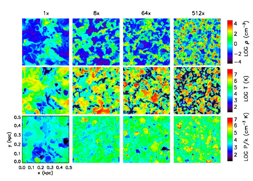
Figure 1.— (From top to bottom) gas density, temperature, and thermal pressure in the midplane of our four ISM models. Each column corresponds to a single model as indicated at the top of each column: (from left to right), 1, 8, 64, and 512 times the Galactic SN rate. The colorbars shown on the right apply to all models.

Figure 2.— (From top to bottom) Probability distribution functions of (a) gas density, (b) temperature, and (c) thermal pressure near the midplane ($|z|\leq 125$ pc) of all models showing fractional volumes contained in logarithmic bins. The 1x, 8x, 64x, and 512x models are shown in solid, dotted, dashed, and dot-dashed curves, respectively.

Figure 1 displays (from top to bottom) gas density, temperature, and thermal pressure in the midplane of the four ISM models. Figure 2 shows probablity distribution functions for those variables. As in the Galactic SN rate model discussed in Paper I, the three classical phases of the ISM are present in every model, with cold, dense filaments surrounded by warm gases that in turn are embedded in hot media. However, their volume fractions vary as a function of the SN rate: The hot and cold phases increase in volume with increasing SN rate, while the volume occupied by the warm phase generally decreases (Fig. 2b). Interestingly, the gas fraction in the thermally unstable range of temperatures (200 $\lesssim T\lesssim$ 7000 K) increases steadily with the SN rate (Fig. 2b), reflecting more dynamic ISM with higher SN rates. More subtle differences are also found. For example, the mean density of the hot gas becomes progressively higher as the SN rate increases (Fig. 2a), likely caused by an increased level of turbulent diffusion off dense shells and filaments where SN explosions occur more frequently (de Avillez & Mac Low 2002). Partly due to the increase in density, the overall thermal pressure $P_{\rm ther}$ in the midplane increases with the SN rate (Fig. 2c). Within each ISM model, however, we find that thermal pressure varies within a range of roughly two orders of magnitude (Mac Low et al. 2005). The peak of the pressure distribution in the Galactic SN rate model lies at $\sim$$3\times 10^{3}$ cm^-3 K, close to the mean value measured with C I fine-structure lines (Jenkins & Tripp 2007). Recent SN remnants are associated with thermal pressures higher than the mean, whereas old SN remnants are tied to those that are lower. The dispersion in $P_{\rm ther}$ rises for high SN rate models, where its maximum value reaches $\sim$$10^{7}$ cm^-3 K, close to the value measured near the center of M82 (Strickland & Heckman 2007). Our results are broadly in agreement with the analytic model by Monaco (2004) in which the ISM was modeled as a two-phase medium in pressure equilibrium.

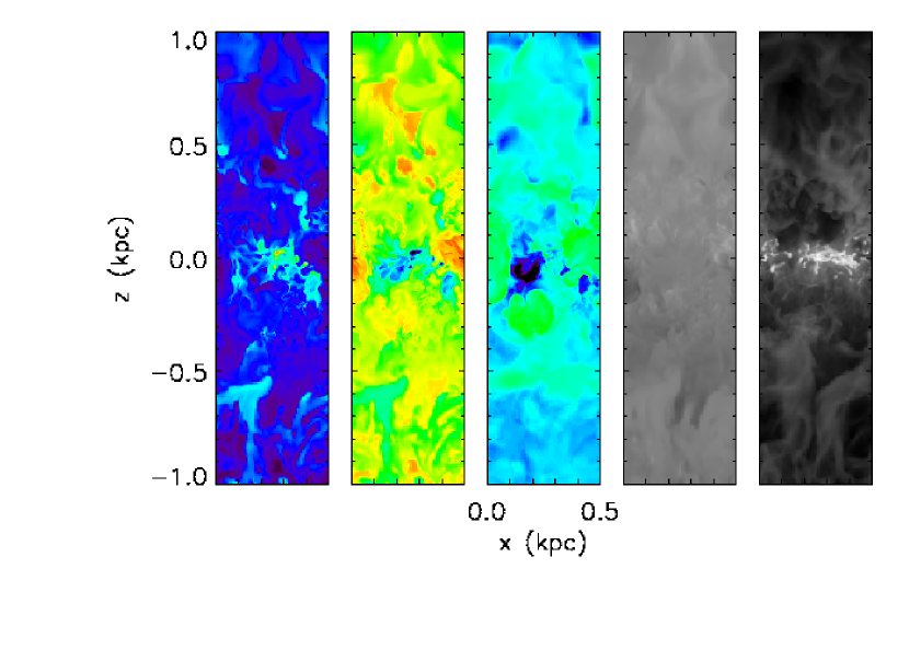
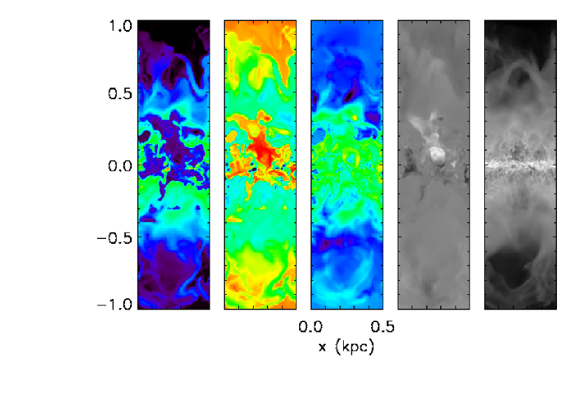
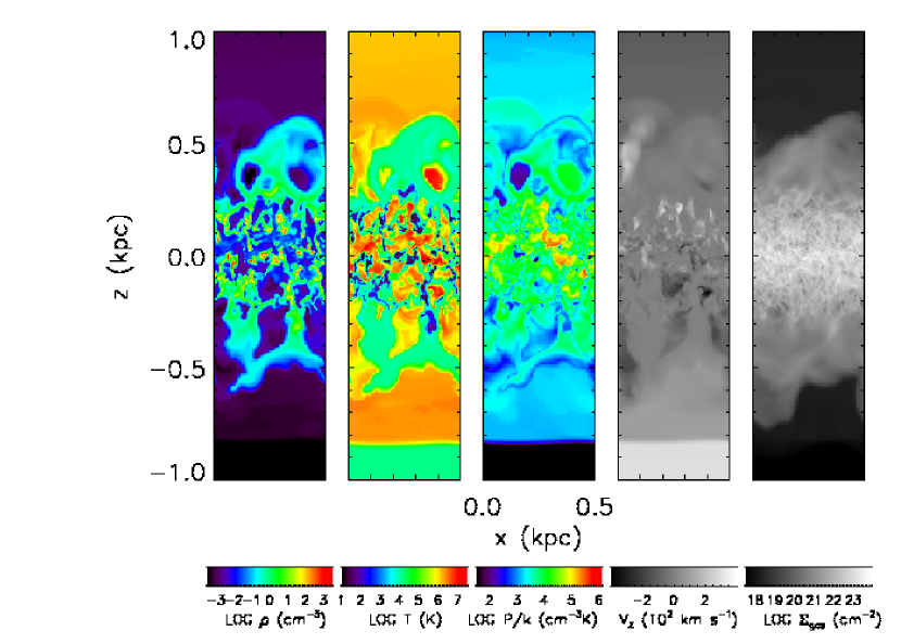
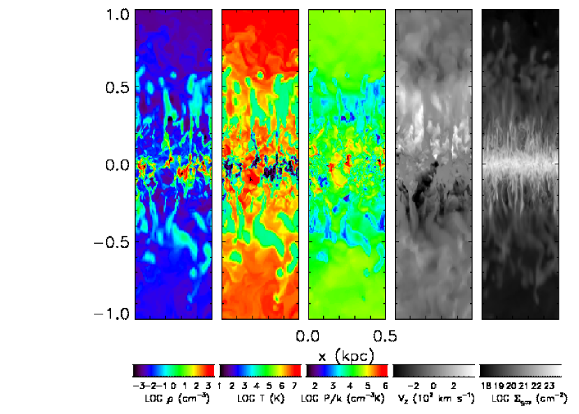
Figure 3.— Vertical distributions of the four ISM models in this paper, (a) 1x, (b) 8x, (c) 64x, and (d) 512x, from a snapshot in time. For each model, (from left to right) slices of gas density, temperature, thermal pressure, and z-component of the velocity, and the projected gas column density are shown for the middle 2 kpc of the models ($|z|\leq 1$ kpc).

The vertical distributions of the ISM models are shown in Figure 3. In all models, correlated SN explosions create superbubbles that vent hot ($T\gtrsim 10^{6}$ K) metal-enriched gas out of the galactic disk into the halo with high velocities ($|v_{\rm z}|\gtrsim 300$ km s^-1). As the SN rate increases, the total gas mass also increases; a gradually larger mass fraction resides in the cold phase rather than in the warm phase. With stronger gravity, we would expect the dense gas to be more confined to the galactic plane, decreasing the disk thickness, while superbubbles would blow out more easily into the halo. On the other hand, the change in the ISM near the galactic midplane should be modest. This is what we find by comparing the two models, 512x and 512xL. The 512x model has higher gas densities in the midplane as well as higher turbulent velocities than those in the 512xL model. In particular, it is worth noting that the 512x model shows superbubble blow-outs, contrary to expectations from some previous work (see § 6 for more details).

4. Turbulent Pressure Distribution

We examine the distribution of turbulent pressures in our models after the systems reach statistical steady states at $t\approx 80$ Myr. Because kinetic energy is distributed over a broad range of wavelengths (see Fig. 8b of Paper I), turbulent pressure is inherently a scale-dependent quantity. To quantify the random (i.e., turbulent) component of the velocity field apart from the bulk motion of the medium, the root-mean-square (rms) velocity dispersion $\sigma$ is measured in the local frame of reference, i.e., the center of mass frame of a selected volume. We choose the entire plane with $|z|\leq 125$ pc, and tile it with small cubical boxes, starting from those with only 2 zones (3.91 pc) on a side. The velocity dispersion within each box is computed from the random component of the velocity field $w$ after subtracting the center-of-mass velocity of the box $\mbox{\boldmath$v$}_{0}$ from the original velocity field $v$. The box size is successively increased twofold until it reaches 128 zones (250 pc) on a side. This procedure enables us to study the velocity dispersion as a function of scale. For each box of a given size, the turbulent rms velocity dispersion $\sigma_{\rm turb,b}$ is calculated by

$$\sigma_{\rm turb,b}^{2}=\frac{1}{M_{\rm b}}\int_{\rm box}\rho\,|\mbox{\boldmath$w$}|^{2}\,dV\;,$$ (2)

where $M_{\rm b}$ denotes the total mass within the box and $\mbox{\boldmath$w$}\equiv\mbox{\boldmath$v$}-\mbox{\boldmath$v$}_{0}$. Similarly, the thermal velocity dispersion $\sigma_{\rm ther,b}$ is computed by replacing $|\mbox{\boldmath$w$}|$ with the local sound speed $c_{\rm s}$. We prefer to use quantities directly related to pressure, so we set

$$\sigma_{\rm ther}=(\sigma_{\rm ther,b}^{2}/\gamma)^{1/2}\,,$$ (3)

$$\sigma_{\rm turb}=(\sigma_{\rm turb,b}^{2}/3)^{1/2}\,,$$ (4)

and

$$\sigma_{\rm tot}=(\sigma_{\rm ther,b}^{2}/\gamma+\sigma_{\rm turb,b}^{2}/3)^{1/2}$$ (5)

for 1D thermal, turbulent, and total velocity dispersions, respectively (see § 6). We hereafter drop the subscript “b” with the understanding that all velocity dispersions are scale-dependent quantities, computed for boxes of a particular size. Similarly, we define the total pressure $P_{\rm tot}$ as the sum of thermal ($P_{\rm ther}=nkT$) and turbulent ($P_{\rm turb}=\rho\,\sigma_{\rm turb}^{2}$) pressures. Below we report our findings on the distributions of turbulent pressure found from this analysis.

4.1. Pressure Equilibrium at Fixed SN Rate

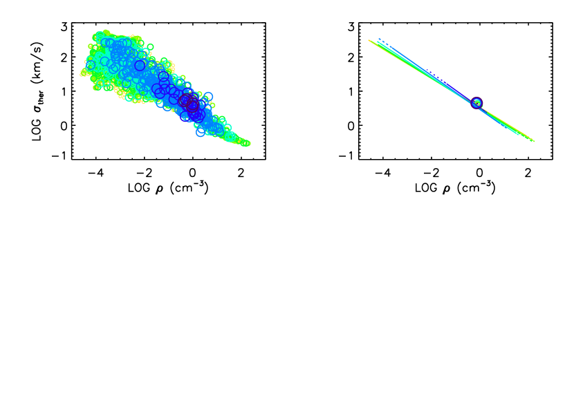
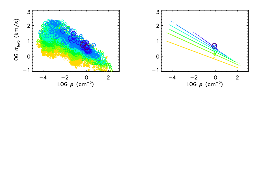
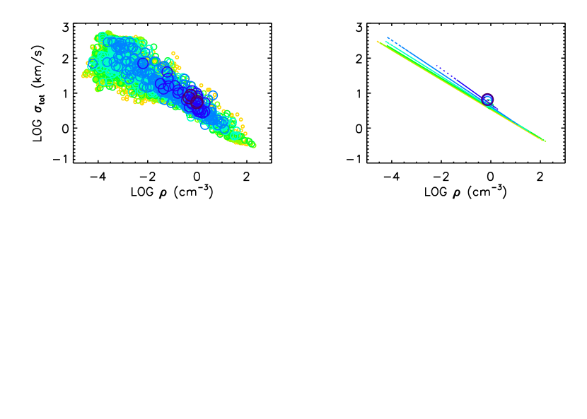
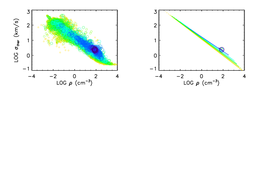
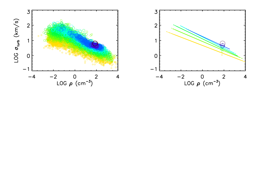
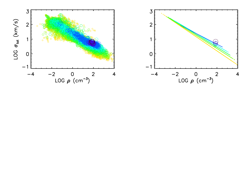
Figure 4.— Mass-weighted (a) thermal, (b) turbulent, and (c) total velocity dispersions plotted against average densities of the boxes. The data are taken near the midplane of our Galactic SN rate model for various box sizes over which the velocity dispersions were computed. Small yellow corresponds to the smallest cubic boxes with 3.91 pc on a side, and purple to the largest boxes with 125 pc on a side. The plots on the right-hand-side display linear regressions of the corresponding plots in the left column, row by row. On a log-log plot, the distribution of points can be characterized by a slope of $-1/2$, implying a nearly constant total pressure. In (b) and (c), the velocity dispersion increases with scale because, as the box size increases, larger eddies gradually contribute to the turbulent velocity dispersion. (d)–(f) are similar plots for the 512x model.

In Figure 4, thermal, turbulent, and total velocity dispersions (Eq. 3–5) are plotted against average densities of individual boxes as a function of the box size. The plots on the right-hand-side display linear regressions of the corresponding plots in the left column, row by row. Small yellow circles represent the smallest boxes (3.91 pc on a side), while big purple ones represent the largest boxes (250 pc on a side). The results are presented only for the 1x and 512x Galactic SN rate models at $t\approx 80$ Myr, but we verified that the conclusions in this section hold for all four models throughout their steady-state evolution.

The most striking feature of these plots is that, for low and intermediate densities ($n\lesssim 10$ cm^-3) the mean velocity dispersion, $\bar{\sigma}\propto\rho^{\,-1/2}$, showing isobaric behavior. This is true at every scale for both thermal and total velocity dispersion, and also at large scales for the turbulent velocity dispersion. The idea of thermal pressure balance between phases is not at all new (Field et al. 1969). Indeed, McKee & Ostriker (1977)’s three-phase ISM model was also based on the premise of “rough pressure balance” between phases, motivated in part by Chandrasekhar & Fermi (1953) and Spitzer (1956). What is new and remarkable is that the turbulent pressure is likewise in approximate pressure equilibrium (Fig. 4b) on large scales where $P_{\rm turb}\gtrsim P_{\rm ther}$. In particular, at any given scale, $\sigma_{\rm tot}\propto\rho^{\,-1/2}$, indicating that the total pressure $P_{\rm tot}=\rho\,\sigma_{\rm tot}^{2}$ is nearly constant in the midplane. This implies that different gas tracers, which often probe narrow ranges of gas densities, may find discrepant kinematics (in particular, velocity dispersions) but that there may be an underlying correlation between them. The pressures are in approximate equilibrium, although the gas density and temperature individually vary by $\sim$7 orders of magnitude.

Furthermore, the thermal velocity dispersion is scale-independent, as indicated by the lines in the top-left panel of Figure 4, which lie almost on top of one another. In contrast, the turbulent velocity dispersion increases with scale. As the box size increases, larger eddies gradually contribute to the turbulent velocity dispersion, and $\sigma_{\rm turb}$ increases just as the power spectrum of kinetic energy predicts (§ 4.4). As a result, the thermal pressure dominates the total pressure on small scales, while the turbulent pressure dominates on large scales. At any particular scale, the scatter is about an order of magnitude in $\sigma$, leading to $\sim$2 orders of magnitude scatter in the pressure (see Fig. 7c of Paper I).

4.2. Turbulent Velocity Dispersion vs. SN Rate

4.2.1 Mass-weighted velocity dispersion

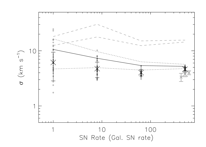
Figure 5.— Turbulent 1D velocity dispersions in boxes with 125 pc sides near the midplane (open circles), plotted against the SN rates in our four models. The changes in the mean values (represented by the X’s and error bars) are minimal across the range of 512 in SN rates. The points in thick grey lines indicate turbulent velocity dispersions measured in the 512xL models with spatial resolutions lower (3.9 pc/cell; left) and higher (0.98 pc/cell; right) than the fiducial model (1.95 pc/cell; middle), offset along the x-axis for clear presentation. The variation of the mean total (thermal plus turbulent) 1D velocity dispersions are shown in solid line, bounded by one sigma dispersions (dotted lines). The grey dashed lines represent the linewidths of H I emission, computed with the entire line profiles (upper curve) and with only the line centers (lower curve), as described in the text.

How does turbulent pressure scale with the SN rate? To answer this question, we compare $\sigma_{\rm turb}$ of the second largest boxes with 125 pc on a side in all models (purple circles in Fig. 4b) and obtain relevant physical quantities averaged over 125 pc scales. (Hence, unless otherwise noted, $\sigma_{\rm turb}$ and $P_{\rm turb}$ henceforth refer to the values computed in boxes with 125 pc sides.) Using these models, we can find how turbulent pressure depends on the SN rate, or after conversion via an appropriate IMF, the star formation rate.

Figure 5 displays the 1D mass-weighted turbulent velocity dispersion against the SN rate for the four SN rates and gas column densities employed in our models. The mean velocity dispersions $\sigma_{\rm turb}$ (in the mass-weighted rms sense) and their standard deviations are given in Table 2 The changes in the mean values are minimal across the range of 512 in SN rates: the best-fit line has the form

$$\sigma_{\rm turb}=(5.6\pm 0.8)\,\dot{\Sigma}_{*,1}^{\;\,-0.045\,\pm\,0.033}\;\,{\rm km\;\rm s}^{-1}\,.$$ (6)

The variation of the mean total (i.e., thermal plus turbulent) 1D velocity dispersions is shown in solid line, bounded by one sigma dispersions (dotted lines). For the mean values for this quantity given in Table 2 the 3D velocity dispersions are 8–18 km s^-1, comparable to the sound speed of the warm gas. The scatter in the velocity dispersion decreases with increasing SN rate.

Table 2Results from the ISM simulations

model	$\sigma_{\rm turb}$	$\sigma_{\rm tot}$	$\sigma_{\rm v,H~{}I}$ a	$L_{\rm d,eff}$ b	$f_{\rm w}$
1x	$6.1\pm 3.3$	$10.6\pm 5.9$	12.5	137	0.460
8x	$4.7\pm 1.5$	$7.3\pm 2.4$	17.8	87	0.274
64x	$4.0\pm 0.5$	$5.4\pm 0.9$	12.4	57	0.431
512x	$4.7\pm 0.4$	$5.2\pm 0.5$	14.4	55	0.609

Note. — See text for definitions of the variables.

For a resolution study, we ran the 512xL model with spatial resolutions half (3.91 pc/cell; left) and double (0.98 pc/cell; right) that of the fiducial model (1.95 pc/cell; middle). The turbulent velocity dispersions measured in these models are indicated by the error bars in thick grey lines without open circles, offset along the x-axis for clear presentation. The velocity dispersions are $3.3\pm 0.6$, $3.8\pm 0.4$, and $4.0\pm 0.3$ km s^-1 for the low, intermediate and high resolution models, respectively. Therefore, although the 512xL models have not fully converged, the velocity dispersion is likely converging to a finite value at infinite resolution, since factor of two changes in resolution led to only $\sim$24% and $\sim$5% increases in the velocity dispersion, with rapidly declining fractional changes. Since the 512xL model is associated with the highest mean density and hence most affected by resolution-dependent effects, we expect better convergence in the other three models.

4.2.2 H I linewidths

High-resolution H I emission maps of nearby, almost face-on galaxies are now available (e.g., Petric & Rupen 2007; Tamburro et al. 2008). These observations show how the H I line widths and shapes change as a function of the galactocentric distance, gas density, distance from spiral structure, and star formation rate. Hence, they provide important constraints on the dominant driving mechanism of the neutral gas.

The brightness temperature, $T_{b}$, is computed by (e.g., Spitzer 1978)

$$T_{b}\,(w)=(5.49\times 10^{-19}\mbox{ K})\left(\frac{N_{{\rm H~{}I}}}{\Delta w}\right)\left(\frac{1-e^{-\tau_{w}}}{\tau_{w}}\right)\,,$$ (7)

where $w$ is the velocity offset from the 21 cm line center, $N_{{\rm H~{}I}}$ is the column density of H i in cm^-2, $\Delta w$ is the velocity width in km s^-1 that we take to be 2.5 km s^-1, which was the velocity resolution in Petric & Rupen (2007), and the velocity-dependent optical depth is given by

$$\tau_{w}=5.49\times 10^{-19}\left(\frac{N_{{\rm H~{}I}}\;e^{-(w/b)^{2}}}{\pi^{1/2}\,b\,T}\right)\,,$$ (8)

where the Doppler linewidth $b=(2kT/m)^{1/2}$ in units of km s^-1. Since we do not follow the multiple species of hydrogen explicitly in our simulations, our estimate of $N_{{\rm H~{}I}}$ is based on simple temperature cutoffs. Specifically, we assume that 100% of hydrogen between 50 and 7000 K exists as H I, while the neutral fraction increases linearly from 30 to 50 K. Below 30 K, hydrogen is assumed to be fully molecular. Note that the H I linewidths are generally larger than the turbulent velocity dispersions. This happens because the bulk of the highest density gas, associated with the lowest velocity dispersion, is molecular and so excluded in the calculation of the former quantity. The uncertainty in H II fraction and in H₂ fraction affect the line profiles in the broad wings and in the centers, respectively.

Figure 6 displays the 21 cm H I emission line profiles for the four ISM models as viewed face-on. With the exception of the 8x model, the line shapes are similar to the universal profile found by Petric & Rupen (2007). As shown, the profiles are wider than single Gaussian fits. The broad wings may be due to the warm component of the neutral gas.

We estimate the linewidth, $\sigma_{\rm v,H~{}I}$, by fitting a single Gaussian to each line profile (grey dashed curves). The Gaussian fits poorly match the line profiles in all models (although it is particularly bad for the 8x model), because of the broad wings, so we additionally fit only the central $\pm 15$ km s^-1 of the line profiles with narrower Gaussian functions shown in grey dotted lines. The broad wings in the 8x model are due to warm gases that are more prominent at lower temperatures ($4000\lesssim T\lesssim 7000$ K) than in the other models (see Fig. 2b). If we set the maximum cutoff temperature for neutral gas to 4000 K instead of 7000 K, the wings show substantially decreased flux as in the other models. On the other hand, removing the gas at high altitudes ($|z|\geq 0.25$ kpc) does not affect the line profile, which indicates that the broad wings are not caused by a galactic wind.

We find that the linewidths (fit to the central $\pm 15$ km s^-1) $\sigma_{\rm v,H~{}I}$ are nearly constant across a wide range of SN rates as given in Table 2, similar to the behavior of the mass-weighted velocity dispersions. These linewidths are comparable to the velocity dispersions found by Agertz et al. (2008) in global galaxy models. They attributed the turbulent motions to global non-axisymmetric modes and cloud-cloud tidal interactions and merging. We find that SN explosions drive turbulent motions that are at least comparable in terms of energy. The H I linewidths, associated with only neutral hydrogen, are systematically higher than the mass-weighted velocity dispersions. Hence, using H I linewidths to infer the overall velocity dispersion may lead to an overestimate. Our results are consistent with the observed near constancy of line-of-sight velocity dispersions with the galactocentric radius (Dickey et al. 1990; Kamphuis 1993), and extend the numerical results of Dib et al. (2006) to stratified interstellar media with gas surface densities increasing with SN rate.

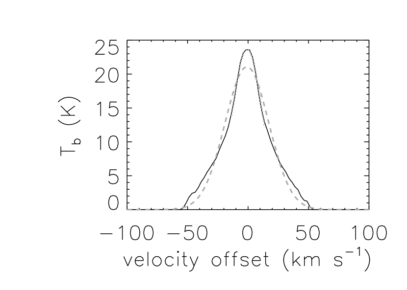
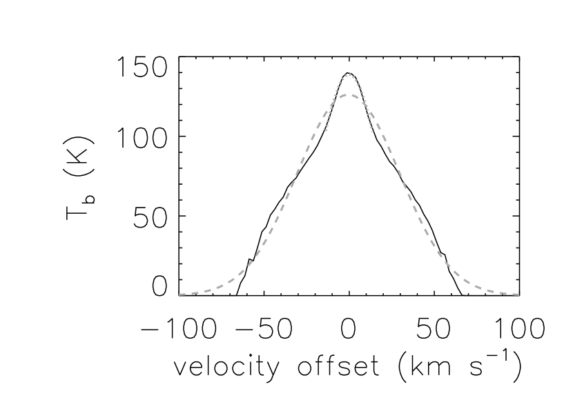
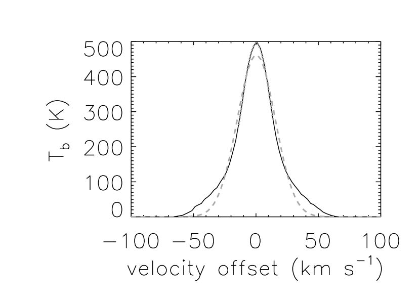
Figure 6.— H I line profiles in the four ISM models viewed from the top. (Top row) 1x, 8x, (bottom row) 64x, and 512x models. Single Gaussian function fits, shown in grey dashed curves, poorly match the line profiles, particularly for the 8x model, because of significant broad wings. Hence, we additionally fit only the central $\pm 15$ km s^-1 of the line profiles with narrower Gaussian functions shown in grey dotted line. The H I linewidths measured near the line centers change relatively little as the SN rate goes up. The tiny dip near the emission peak in the 512x model is caused by self-absorption of H I emission.

4.3. Thermal vs. Turbulent Pressures

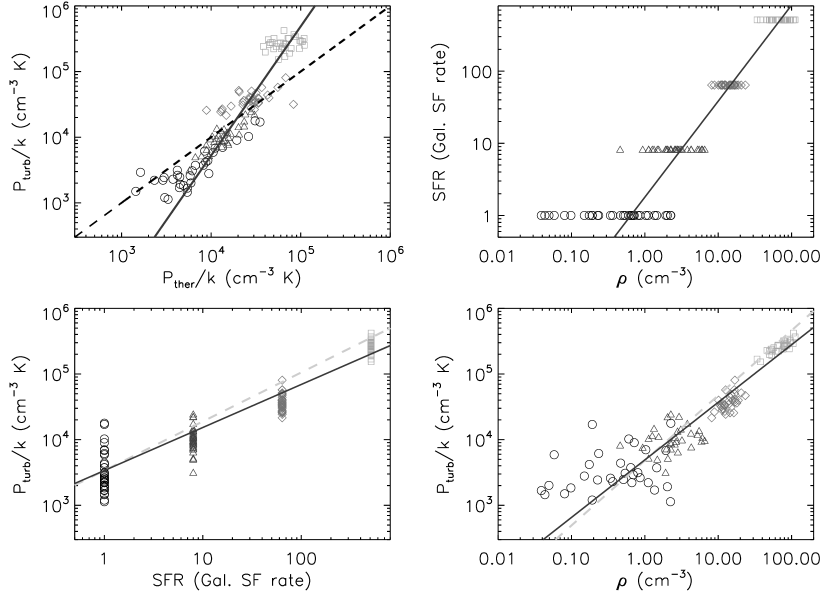
Figure 7.— Turbulent pressure variation in our four models with different SN rates. Displayed are: (a) turbulent vs. thermal pressure, (b) assumed SFR vs. density, (c) turbulent pressure vs. SFR, and (d) turbulent pressure vs. density. Each quantity is evaluated in (125 pc)³ boxes near the midplane of the model galaxies. Different symbols indicate the ISM models: 1x (circles), 8x (triangles), 64x (diamonds), and 512x (squares). In (a), the black dashed line is drawn for $P_{\rm turb}=P_{\rm ther}$. The dark solid lines represent best-fit lines to all four ISM models. The grey dashed lines in (c) and (d) represent the relations expected from the subgrid model if the ratio $\epsilon^{\prime}_{1}/\epsilon_{2}$ is constant, equations (20) and (19), respectively.

Figure 7a shows a remarkably tight correlation between thermal pressure and turbulent pressure (computed in boxes with 125 pc sides) across our ISM models. This arises because higher SN rates naturally lead to increases in both thermal and turbulent pressures. The best-fit line has a slope that is steeper than unity ($1.97\pm 0.13$), implying that the turbulent pressure increasingly dominates at higher SN rates. Note that this does not necessarily mean that turbulent pressure is comparable in magnitude to thermal pressure on all scales. Turbulence from large-scale motions (i.e., scales larger than our box size that are not well modeled by the simulation) may have a significant contribution, and so $P_{\rm tot}/P_{\rm ther}$ may be significantly larger than $\sim$2 on scales above 125 pc.

4.4. Kinetic Energy Spectrum

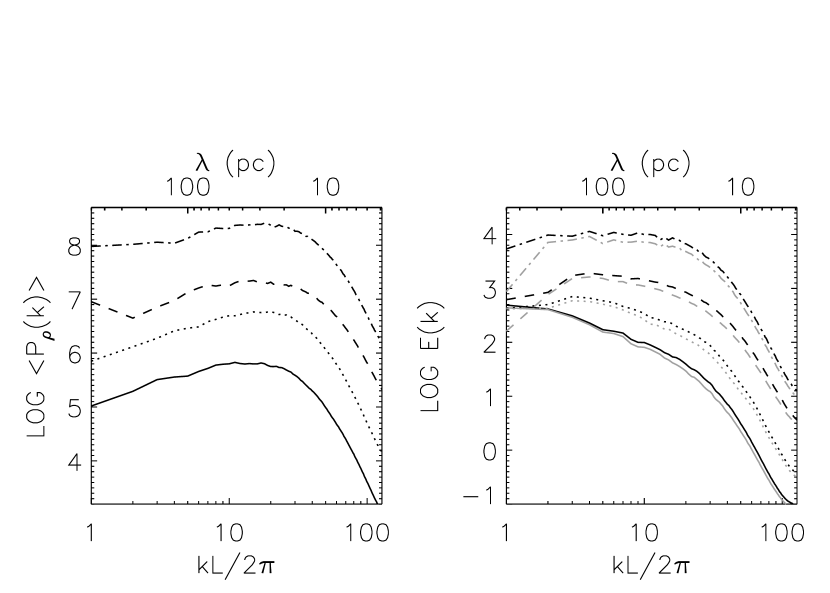
Figure 8.— Left: Angle-averaged density power spectra. Right: Kinetic energy spectra (black) and angle-averaged velocity power spectra (grey). The kinetic energy is distributed over a broad range of wavelengths, but the characteristic scale containing most of the energy shifts to larger wavenumbers (shorter wavelengths) as the SN rate increases.

In Paper I, it was shown that the kinetic energy in an explosion-dominated medium is distributed over a broad range of wavelengths. Then how do the characteristic scales of the density and kinetic energy distributions change as a function of SN rate? Figure 8 displays angle-averaged density power spectra (left) as well as kinetic energy spectra in black and angle-averaged velocity power spectra in grey (right); see Paper I for details on how they are computed. As in the Galactic SN rate model, the velocity power spectra deviate significantly from the Kolmogorov spectrum, which is applicable to an incompressible medium driven at a single large scale: these assumptions are not applicable to the ISM driven by supersonic shocks on a range of scales. It is clear from Figure 8 that the scale containing most of the kinetic energy shifts to larger wavenumbers (smaller wavelengths) with increasing SN rate. We quantify this change by computing the effective driving scale defined by

$$L_{\rm d,eff}\equiv\frac{2\pi\int k^{-1}E_{k}\,dk}{\int E_{k}\,dk}\;.$$ (9)

We find the values of $L_{\rm d,eff}$ given in Table 2. The best-fit line has a form $L_{\rm d,eff}\approx(126\pm 18\;{\rm pc})\,(\dot{\Sigma}_{*}/\dot{\Sigma}_{*,1})^{\;-0.15\,\pm\,0.03}$, where $\dot{\Sigma}_{*,1}$ is the SN rate per unit area in the 1x model. It should be remembered that we are dealing only with SN driven turbulence. Large-scale turbulence driven by, e.g., self-gravity may contribute to turbulence on larger scales, so that the combined power spectrum may be more or less continuous out to kiloparsec scales, as observed (e.g., Elmegreen et al. 2001).

5. Subgrid Model for Turbulent Pressure

5.1. Basic Features

A genuine, three-dimensional, cosmological model that properly includes SN feedback would need to encompass an unrealistically large dynamic range, starting from length scales responsible for galaxy formation ($>$1 Mpc) down to those relevant to star formation ($<$1 pc). The resulting spatial dynamic range of at least $10^{6}$ requires computational resources currently impracticable. Past attempts to circumvent this problem include analytic approaches based on McKee & Ostriker (1977)’s multiphase model of the ISM (e.g., Efstathiou 2000) and semi-analytic methods with parametrized prescriptions for star formation and feedback (Kauffmann et al. 1993; Somerville & Primack 1999; Cole et al. 2000).

An alternative method is to use subgrid (or subresolution) models (Yepes et al. 1997; Springel 2000; Semelin & Combes 2002; Springel & Hernquist 2003). In these models, one represents the physics unresolved in the global model (i.e., turbulent motions on small scales) by an analytic prescription. Relevant physical quantities are evolved on a subgrid scale, and their appropriate averages yield a simple description of the medium on the smoothing scale. The desired net effect is to have a large-scale simulation on a coarse grid, indistinguishable from the one in which all motions are resolved down to parsec scales.

Our approach is inspired by the subgrid model described by Springel (2000), which assumes that turbulent motions below resolved scales produced by SN feedback can be represented by a second reservoir of internal energy of the gas, a term that helps to support the gaseous medium in the absence of substantial thermal support. Nonlinear physical processes such as shock compressions, radiative cooling and thermal instability shape the properties of interstellar turbulence. Hence, a subgrid model based on heuristic analytic arguments should be checked by direct numerical simulations that include the relevant physics. For this reason, we explicitly calibrate our subgrid model against the results of our local ISM simulations. The subgrid model is therefore based on the results of our high-resolution local ISM models that resolve turbulent motions of the gas. In a sense, we imagine an entire model galaxy on a coarse grid ($\sim$100 pc spatial resolution), and within it, identify each cell with a box with side $\sim$100 pc taken from one of our local models.

The key parameter in our subgrid model is the turbulent pressure. Local ISM models described in this paper and elsewhere suggest that turbulent pressure is more important than either thermal (Boulares & Cox 1990; Lockman & Gehman 1991) or magnetic pressures (Kim 2004; de Avillez & Breitschwerdt 2005) in most ISM conditions. This suggests that cosmological subgrid models should include a term for the turbulent pressure, rather than focusing on thermal pressure alone. Here we suggest a simple extension where we add an additional energy term in the fluid equation to describe the turbulent energy on scales not resolved by the simulation (Joung 2006; Bryan 2007). Two characteristics of our local ISM models are conducive to developing such a subgrid model for turbulent pressure as a way to represent small-scale motions. First, $>$90% of the total kinetic energy is on scales below 200 pc (Paper I). In current high-resolution cosmological simulations, therefore, most of the turbulent energy lies on scales smaller than a resolution element, and there is hope that such a model assuming a separation of scales would work. Second, the turbulent pressure is nearly constant on scales greater than $\sim$100 pc (§ 4.1), which suggests that for a given SN rate, a single value of turbulent pressure can characterize the medium regardless of the local gas density, albeit with the scatter shown in Figure 4b (left).

In our subgrid model, the pressure is given by

$$P=P_{\rm ther}+P_{\rm turb}=(\gamma-1)\,\rho\,(e+q)$$ (10)

where $e$ is the specific thermal energy density, while $q=\sigma_{\rm turb}^{2}$ is the specific turbulent energy density. Essentially, we require an additional energy equation that is similar to the one for thermal energy but includes a source term reflecting the turbulent energy input from SNe instead of thermal heating terms, and a sink term corresponding to the decay of turbulence instead of radiative cooling terms:

$$\frac{dq}{dt}=-(\gamma-1)\,q\mbox{\boldmath$\nabla$}\cdot\mbox{\boldmath$v$}+\epsilon_{1}\frac{\epsilon_{\rm fb}\,\dot{\rho}_{*}}{\rho}-\epsilon_{2}\frac{q^{3/2}}{L}\,.$$ (11)

The star formation rate per unit volume, $\dot{\rho}_{*}=c_{*}(\rho/t_{\rm dyn})$, where $t_{\rm dyn}=[3\pi/(32G\rho)]^{1/2}$ is the dynamical time and the star formation efficiency per dynamical time, $c_{*}\approx 0.02$–$0.03$ (Krumholz & Tan 2007). The local energy input due to SNe, $\dot{\varepsilon}_{\rm in}=\epsilon_{\rm fb}\dot{\rho}_{*}$, where the energy input per unit stellar mass, $\epsilon_{\rm fb}=4\times 10^{48}$ erg M${}_{\odot}^{-1}$ if the initial mass function (IMF) with a slope of $-1.5$ between 0.1 and 40 M_⊙ and all stars with mass $>$8 M_⊙ exploding as SNe. The turbulent energy is assumed to decay at a rate proportional to $q/t_{\rm cross}$ where $t_{\rm cross}=L/q^{1/2}$ is the crossing time at the turbulent driving scale (Mac Low 1999); we assume $L\approx L_{\rm d,eff}$, calculated in § 4.4.

The two dimensionless parameters $\epsilon_{1}$ and $\epsilon_{2}$ are selected to match local ISM simulations. The first of these parameters, $\epsilon_{1}$, measures the efficiency of conversion of SN energy into kinetic motions, which may depend on, e.g., the density and metallicity of the surrounding medium (e.g., Thornton et al. 1998). We expect $\epsilon_{1}$ to decrease with increasing SN rate. The second parameter, on the other hand, may be more or less constant; Mac Low (1999) found $\epsilon_{2}\simeq 0.84$ for a range of energy injection rates and driving scales from a large set of hydrodynamic and magnetohydrodynamic simulations with an isothermal equation of state.

The thermal energy equation, in turn, is given by

$$\frac{de}{dt}=-(\gamma-1)\,e\mbox{\boldmath$\nabla$}\cdot\mbox{\boldmath$v$}+\frac{n\Gamma-n^{2}\Lambda}{\rho}+(1-\epsilon_{1})\frac{\epsilon_{\rm fb}\,\dot{\rho}_{*}}{\rho}+\epsilon_{2}\frac{q^{3/2}}{L}\,,$$ (12)

where $n\Gamma(\rho,e,I_{\rm isrf})$ and $n^{2}\Lambda(\rho,e)$ denote appropriate thermal heating and radiative cooling rates per unit volume, respectively, $n$ is the number density of the gas, and $I_{\rm isrf}$ is the intensity of the interstellar radiation field. The last two terms account for direct thermal heating from SNe and the dissipation of turbulent energy into heat. When combined with the Euler equations, equations (10), (11) and (12) determine the evolution of thermal and turbulent energy densities.

5.2. Calibration with Local ISM Models

We can make simple analytic arguments to see how turbulent pressure is expected to vary as a function of the SN rate. To do this, we assume a steady state, where the energy input rate from SN explosions, $\dot{\varepsilon}_{\rm in}$, is balanced by the dissipation of turbulent motions. We set $dq/dt=0$ and $\mbox{\boldmath$\nabla$}\cdot\mbox{\boldmath$v$}=0$ in equation (11) to obtain

$$\epsilon^{\prime}_{1}(1-f_{\rm w})\,\dot{\varepsilon}_{\rm in}=\epsilon_{2}\,\frac{\rho\,q^{3/2}}{L}\;,$$ (13)

where we write $\epsilon_{1}$ as $\epsilon^{\prime}_{1}(1-f_{\rm w})$ to explicitly account for the dependence on $f_{\rm w}$, the fraction of input energy that goes into driving large-scale ($\gtrsim 100$ pc) motions such as galactic winds, and hence is not captured in the subgrid model. Now, to facilitate comparison with our ISM simulations, where we used the Schmidt-Kennicutt law for the initial conditions (Eq. 1), we adopt $\dot{\varepsilon}_{\rm in}=\epsilon_{\rm fb}\,A(2\rho H_{\rm gas})^{1.4}/(2H_{\rm SN})$, where $H_{\rm gas}$ and $H_{\rm SN}$ are vertical scale heights for gas and SNe, respectively. The turbulent pressure is then given by

$$P_{\rm turb} = \rho\,q=\rho\left(\frac{\epsilon^{\prime}_{1}(1-f_{\rm w})}{\epsilon_{2}}\frac{\dot{\varepsilon}_{\rm in}L}{\rho}\right)^{2/3}$$ (14)

$$= \,\mathcal{C}\,[(1-f_{\rm w})\,H_{\rm gas}^{7/5}\,L]^{2/3}\,\rho^{\,19/15}\,,$$ (15)

where the combination of parameters,

$$\mathcal{C}\equiv\left(\frac{2^{0.4}\,\epsilon^{\prime}_{1}}{\epsilon_{2}}\,\frac{\epsilon_{\rm fb}\,A}{H_{\rm SN}}\right)^{2/3}\,.$$ (16)

Now, consider each factor in brackets on the RHS of equation (14). The driving scale has already been computed (Eq. 9); we take $\,L\approx L_{\rm d,eff}\propto\dot{\Sigma}_{*}^{\;-0.15\,\pm\,0.03}\propto\dot{\varepsilon}_{\rm in}^{\;-0.15\,\pm\,0.03}$, if $\epsilon_{\rm fb}$ and $H_{\rm SN}$ change little with the SN rate. To compute the gas scale height, $H_{\rm gas}$, we plot the SN rate (normalized to the Galactic rate) as a function of gas density in Figure 7b. If $H_{\rm gas}$ is constant across our models, the energy input rate will scale with the gas density in the same way as it varies with the gas surface density ($\,\dot{\Sigma}_{*}\propto\rho^{\,1.4}\,$). This is indeed close to what we find for the best-fit line shown in Figure 7b:

$$\dot{\Sigma}_{*}=(1.79\pm 0.17)\,\dot{\Sigma}_{*,1}\,\left(\frac{\rho}{\rho_{1}}\right)^{\,1.33\,\pm\,0.03}\;,$$ (17)

where $\rho_{1}\simeq 0.7$ cm^-3 is the mean density in the midplane of the 1x model. From this relation and $H_{\rm SN}\approx 90$ pc, we infer a nearly constant gas scale height of 170 pc $(\dot{\Sigma}_{*}/\dot{\Sigma}_{*,1})^{\,0.04\,\pm\,0.02}$.

To estimate how the fraction of energy driving large scale motions ($f_{\rm w}$) scales with the SN rate, we distinguish between the small-scale, turbulent motions within boxes having 125 pc sides, as examined in § 4, and the bulk motion of these individual boxes. This amounts to comparing the sum of the kinetic energy contained in (mass-weighted) velocity dispersions inside the boxes ($\rho\,\sigma_{\rm turb}^{2}/2$) and that from the center-of-mass velocities of the boxes themselves ($\rho|\mbox{\boldmath$v$}_{0}|^{2}/2$). Using this procedure, we obtain the values of $f_{\rm w}$ given in Table 2. This does not contradict our earlier result that almost all the turbulent energy is contained on scales below $\sim$200 pc, because we were then discussing the kinetic energy spectrum in the midplane region only. In fact, if we confine our attention to the region with $|z|\leq 125$ pc and compute the energy fraction in large-scale motions, we obtain significantly smaller values (0.084, 0.065, 0.149, and 0.455). In other words, most of the kinetic energy on large scales comes from the bulk motions at high altitudes: galactic winds. If we fit a straight line through the values of $f_{w}$ given in Table 2, we find

$$1-f_{\rm w}=(0.65\pm 0.15)\,\left(\frac{\dot{\Sigma}_{*}}{\dot{\Sigma}_{*,1}}\right)^{\;-0.06\,\pm\,0.05},$$ (18)

which is effectively a constant.

To study the variation of turbulent pressure in our ISM simulations, we compute $P_{\rm turb}$ in boxes of size (125 pc)³ taken from the midplane region ($|z|\leq 125$ pc) of the four ISM models. The results given in Figure 7c–d show the turbulent pressure depends on the input SN rate as well as the gas density averaged over cubes with 125 pc sides. The expectations from the subgrid model (Eq. 14) assuming constant $\mathcal{C}$ are shown as grey dashed lines in Figures 7c and 7d. The best-fit lines to the data, shown in dark solid lines, have the form

$$P_{\rm turb}\propto\dot{\Sigma}_{*}^{\;0.66\,\pm\,0.04}\;.$$ (19)

and, in terms of the gas density,

$$P_{\rm turb}\propto\rho^{0.88\pm 0.05}\;,$$ (20)

This effective equation of state (EOS) is slightly more compressible than an isothermal EOS, for which $P\propto\rho^{\,1}$. In contrast, much stiffer effective EOSs were adopted in previous subgrid models. For example, Springel (2000) used an EOS of the form $P\propto\rho^{\,2}$, obtained by assuming that all SN energy first goes into turbulent energy and then converts to thermal energy with an efficiency that depends specifically on gas density ($\epsilon_{1}=1$ and $\epsilon_{2}\propto\rho^{\,-1/2}$ in our notation). In the hybrid multiphase model developed by Springel & Hernquist (2003), hot gas from SNe delays radiative cooling and provides the necessary additional pressure. Here, the effective EOS was also stiffer than isothermal above a threshold density ($\sim$0.1 cm^-3), where star formation was assumed to switch on. Our result indicates that SN-driven turbulence does not naturally provide a stiff EOS on 100–200 pc scales but rather that the effective EOS of the ISM averaged over these scales is slightly sub-isothermal (see § 6 for further discussion).

The simulation results deviate slightly from the naive expectations based on constant $\mathcal{C}$, especially in the models for starbursts (the 64x and 512x models). This suggests that $\mathcal{C}$ may be close to but not exactly a constant. Combining the scaling relations we have found, we obtain

$$\mathcal{C}\propto\dot{\varepsilon}_{\rm in}^{\;-0.55\,\pm\,0.07}\;,$$ (21)

or $\epsilon^{\prime}_{1}\propto\dot{\varepsilon}_{\rm in}^{\,-0.82\,\pm\,0.11}\propto\rho^{\,-1.15\,\pm\,0.15}$ for a constant $\epsilon_{2}$. Hence, a smaller fraction of SN energy is used to drive kinetic motions as the SN rate (and the mean gas density) increases, although the dependence is weak.

We must mention several caveats that may affect our conclusion. Our ISM simulations do not include magnetic fields or self-gravity of gas, which can change the structure and the pressure distribution of the medium, especially in the dense regions. In principle, unphysical cooling of numerical origin may be important, particularly in the 64x and the 512x models. This would occur at the interfaces between hot and cold gas, which are inevitably wider than the physical value, and so contain more gas at intermediate temperatures between $10^{4}$ K and $10^{6}$ K that is subject to strong radiative cooling than they physically should (e.g., Mac Low et al. 1989). Such cooling could yield values of $P_{\rm turb}$ that are lower than the correct values. However, the resolution study discussed in § 4.2 shows that this is a surprisingly minor problem in practice. An alternative method to examine this issue would be to use a tracer field (Yabe & Xiao 1993) to suppress the excessive cooling in young SN remnants as in previous work (Mac Low & Ferrara 1999; Fujita et al. 2004), after appropriately modifying the criterion for suppression for the case of multiple discrete SN explosions.

6. Discussion

Comparison with Chandrasekhar’s formula for the effective sound speed.

In § 4, we have used $P_{\rm tot}=\rho\,(\sigma_{\rm ther}^{2}+\sigma_{\rm turb}^{2})=\rho\,(\sigma_{\rm ther,b}^{2}/\gamma+\sigma_{\rm turb,b}^{2}/3)$. The reader may wonder why this is the appropriate expression. For example, compare it with the expression $c_{\rm s,eff}^{2}=c_{\rm s}^{2}+\langle u^{2}\rangle/3$ where $c_{\rm s,eff}$ is the effective sound speed, which Chandrasekhar (1951) used to extend Jeans’s analysis to an infinite homogeneous turbulent medium. One immediately notices that, in his formulation, $c_{\rm s}^{2}$ was used instead of $c_{\rm s}^{2}/\gamma$. To understand this, we propose the following thought experiment. If we have two parcels of gas at the same temperature but with two different adiabatic indices (e.g., $\gamma$ = 5/3 and 7/5), they should have the same pressure (since $P_{\rm ther}=nkT$). However, when you try to compress the gases, they have different resistance to the compression, i.e., the one with higher $\gamma$ is more difficult to compress and hence their sound speeds differ. The first case is relevant to pressure equilibrium in our models; the second to Chandrasekhar’s problem. Essentially, our problem is a pressure issue, while Chandrasekhar’s is a communication timing issue (the Jeans stability criterion says $t_{\rm cross}<t_{\rm dyn}$).

Large-scale turbulence driving.

We argued that most of the kinetic energy due to SN-driven turbulence can be contained in resolution elements (with size of 100–200 pc) of cosmological simulations, hence allowing the approach of subgrid modeling. In reality, however, there are numerous other energetic processes that occur on larger scales that may affect the dynamics. An example would be gravitational instability induced by spiral structure such as the magneto-Jeans instability (Kim & Ostriker 2002). Li et al. (2005a, 2006) argued, using an isothermal equation of state to represent stellar feedback, that gravity controls when and where star formation occurs, and reproduced the Schmidt-Kennicutt law with realistic star formation thresholds. The use of a subgrid model for interstellar turbulence does not mean that we ignore these larger-scale, possibly gravity-induced motions. Rather, we are making an assumption that the characteristic lengths at which these two processes operate are sufficiently far apart that they can be treated separately in global models. One way to test this hypothesis is to compare simulated and observed column density power spectra (Elmegreen et al. 2001) for both local and global simulations of galaxies.

Observed linewidths in ULIRGs.

High velocity dispersions in molecular gas, $\sigma_{\rm CO}\approx 100$ km s^-1, were observed in ultraluminous infrared galaxies (ULIRGs) such as Arp 220 (Downes & Solomon 1998). Murray et al. (2005; see also Thompson et al. 2005) suggested that in extreme starbursting systems such as ULIRGs, the ambient high density gas impedes the expansion of SN remnants, drastically lowering the efficiency with which SN energy escapes the host galaxy. Their model does not include the effect of superbubbles: correlated SNe with high $n_{\rm SN}$ may decrease the ambient density near explosion sites, and the overall radiative cooling rate in such explosions may be significantly reduced. In our models with high SN rates, SN explosions near the midplane drive large-scale motions about as effectively as in models with lower SN rates. The fraction of energy stored in turbulent motions as opposed to heat increases with SN rate. We note that Fujita et al. (2008) recently found that extremely superthermal linewidths ($\sim$320 km s^-1) in Na I absorbing gas could be reproduced using a model for an energy-driven superbubble with a spatial resolution of $\leq 0.2$ pc, assuming a single central starburst region and axisymmetry. The energy input rate of our 512x model is $\sim$1.3$\times$10⁴¹ erg s^-1, comparable to the lowest mechanical luminosity model in Fujita et al. (2008).

Effective equation of state.

The models presented in this paper demonstrate that a stiff EOS does not result from SN explosions in a stratified ISM, since the effective EOS including turbulent pressure across the local ISM models is close to isothermal. In the past, stiff EOSs were proposed as a way of preventing the collapse of disk galaxies to unphysically small radii in cosmological simulations. However, Li et al. (2005b) showed that such collapse was due to violation of the Jeans criterion (Truelove et al. 1997) in low resolution simulations, and that fully resolved, isothermal disks do not collapse. Simulations of full galaxies including our sub-grid model will reveal whether there are further effects that a stiffer equation of state would better reproduce.

Limitation of the steady state assumption.

The subgrid model developed in this paper can be easily implemented in cosmological simulations. However, our approach is limited by the assumption of constant SN rate; we dealt only with steady state systems. The model is appropriate if the characteristic timescale $\tau_{\rm SF}$ over which the SN (SF) rate averaged over $\sim$100 pc regions changes appreciably is much longer than the time it takes for the system to reach a steady state ($\sim$60 Myr in our simulations). The assumption is valid, e.g., in merging galaxies, where $\tau_{\rm SF}$ is on the order of 0.1–1 Gyr.

7. Summary

Interstellar turbulence is thought to play a major role in the formation and support of molecular clouds and the regulation of the size, thickness, and star formation rate of galactic disks (Mac Low & Klessen 2004; Elmegreen & Scalo 2004). We examined the physical characteristics of the ISM by constructing high-resolution 3D models of a stratified ISM driven by both correlated and isolated SN explosions. A suite of numerical experiments, each with a simulated volume of (0.5 kpc)²$\times$(10 kpc), were performed using an adaptive mesh code at a maximum spatial resolution of 1.95 pc; they included vertical gravity and parameterized heating and cooling. The simulations cover wide ranges of supernova rates and vertical gas column densities, with initial conditions based on the Schmidt-Kennicutt law (Kennicutt et al. 1998, 2007).

We find that the turbulent velocity dispersion is inversely proportional to the square root of the local density: $\sigma_{\rm turb}\propto\rho^{-1/2}$ on $\gtrsim$50 pc scales. The turbulent pressure, $\rho\,\sigma_{\rm turb}^{2}$, in such a medium is nearly constant at a given scale, even though the gas density varies by about seven orders of magnitude. This suggests that, for a given SN rate, a single value of turbulent pressure can characterize the medium regardless of the local gas density. When combined with the finding in Paper I that $>$90% of the total kinetic energy is contained on scales below 200 pc, the two charateristics of the ISM are conducive to developing a subgrid model for turbulent pressure as a way to represent small-scale motions. One such model was developed in this paper and explicitly calibrated using the local ISM simulations.

We find that the mass-weighted velocity dispersion $\sigma_{\rm turb}$ and the simulated H I linewidth $\sigma_{\rm v,H~{}I}$ are nearly constant across a range of 512 in SN rate (see Table 2 for values). In other words, the appropriate equation of state for $P_{\rm turb}$ in gas averaged over $\sim$100 pc regions is close to isothermal. In our highest supernova rate model, superbubble blow-outs occur, and the turbulent pressure on large scales is $\gtrsim$4 times higher than the thermal pressure.

We propose a subgrid model that naturally includes the effect of turbulence in large-scale simulations, at least as far as we understand it from our small-scale models, and furnishes a sound, physically motivated prescription for including the effect of SN feedback in cosmological simulations. It treats turbulence as strictly a pressure term, although small-scale effects on the star formation rate could, in principle, be included in a statistical way. The advantage of this type of approach is that we prescribe the subgrid model from what we know (bottom-up) rather than what we need in order to resolve current problems in cosmological simulations (top-down).

References

- Adelberger et al. (2003) Adelberger, K. L., Steidel, C. C., Shapley, A. E., & Pettini, M. 2003, ApJ, 584, 45
- Agertz et al. (2008) Agertz, O., Lake, G., Teyssier, R. et al. 2008, MNRAS, in press (arXiv:0810.1741)
- Aguirre et al. (2005) Aguirre, A., Schaye, J., Hernquist, L. et al. 2005, ApJ, 620, L13
- Banerjee et al. (2007) Banerjee, R., Klessen, R. S., & Fendt, C. 2007, ApJ, 668, 1028
- Benson et al. (2003) Benson, A. J., Bower, R. G. et al. 2003, ApJ, 599, 38
- Bertschinger (1998) Bertschinger, E. 1998, ARA&A, 36, 599
- Binney & Tremaine (1987) Binney, J., & Tremaine, S. 1987, Galactic Dynamics (Princeton: Princeton Univ. Press)
- Boulares & Cox (1990) Boulares, A., & Cox, D. P., 1990, ApJ, 365, 544
- Bower et al. (2006) Bower, R. G. et al. 2006, MNRAS, 370, 645
- Bryan (2007) Bryan, G. L. 2007, Proc. CRAL-Conf. Ser. I ”Chemodynamics: from First Stars to Local Galaxies”, Lyon, France, Eds. Emsellem, Wozniak, Massacrier et al., Champavert, EAS Publ. Ser., Vol. 24 (arXiv:0707.1856)
- Bryan & Norman (1998) Bryan, G. L., & Norman, M. L. 1998, ApJ, 495, 80
- Carroll et al. (2008) Carroll, J. J., Frank, A., Blackman, E. G. et al. 2008, submitted (arXiv:0805.4645)
- Cen et al. (1994) Cen, R., Miralda-Escude, J., Ostriker, J. P., & Rauch, M. 1994, ApJ, 437, L9
- Cen & Ostriker (2000) Cen, R. & Ostriker, J. P. 2000, ApJ, 538, 83
- Cen et al. (2005) Cen, R., Nagamine, K., & Ostriker, J. P. 2005, ApJ, 635, 86
- Chandrasekhar (1951) Chandrasekhar, S. 1951, Proc. Royal Soc. London A, 210, 26
- Chandrasekhar & Fermi (1953) Chandrasekhar, S., & Fermi, E. 1953, ApJ, 118, 113
- Cole et al. (2000) Cole, S., Lacey, C. G., Baugh, C. M., & Frenk, C. S. 2000, MNRAS, 319, 168
- Croton et al. (2006) Croton, D. J., Springel, V. et al. 2006, MNRAS, 365, 11
- Dalgarno & McCray (1972) Dalgarno, A., & McCray, R. A. 1972, ARA&A, 10, 375
- de Avillez & Berry (2001) de Avillez, M. A., & Berry, D. L. 2001, MNRAS, 328, 708
- de Avillez & Mac Low (2002) de Avillez, M. A., & Mac Low, M.-M. 2002, ApJ, 581, 1047
- de Avillez & Breitschwerdt (2004) de Avillez, M. A., & Breitschwerdt, D. 2004, A&A, 425, 899
- de Avillez & Breitschwerdt (2005) ——. 2005, A&A, 436, 585
- Dib et al. (2006) Dib, S., Bell, E., & Burkert, A. 2006, ApJ, 638, 797
- Dickey et al. (1990) Dickey, J. M., Hanson, M. M., & Helou, G. 1990, ApJ, 352, 522
- Downes & Solomon (1998) Downes, D., & Solomon, P. M. 1998, ApJ, 507, 615
- Dunkley et al. (2008) Dunkley, J. et al. 2008, ApJ, in press (arXiv:0803.0586)
- Efstathiou (2000) Efstathiou, G. 2000, MNRAS, 317, 697
- Elmegreen et al. (2001) Elmegreen, B. G., Kim, S. & Staveley-Smith, L. 2001, ApJ, 548, 749
- Elmegreen & Scalo (2004) Elmegreen, B. G., & Scalo, J. 2004, ARA&A, 42, 211
- Ferrara (1993) Ferrara. A. 1993, ApJ, 407, 157
- Field et al. (1969) Field, G. B., Goldsmith, D. W., & Habing, H. J. 1969, ApJ, 155, L49
- Fryxell et al. (2000) Fryxell, B., Olson, K., Ricker, P., Timmes, F. X., Zingale, M. et al. 2000, ApJS, 131, 273
- Fujita et al. (2004) Fujita, A., Mac Low, M.-M., Ferrara, A. et al. 2004, ApJ, 613, 159
- Fujita et al. (2008) Fujita, A., Martin, C. L. et al. 2008, ApJ, submitted (arXiv:0803.2892)
- Gazol-Patiño & Passot (2005) Gazol-Patiño, A., & Passot, T. 1999, ApJ, 518, 748
- Gibson et al. (2008) Gibson, B. K., Courty, S., Sanchez-Blazquez, P. et al. 2008, to appear in ”The Galaxy Disk in Cosmological Context,” Proc. IAU 254 (Copenhagen, eds. J. Anderson, J. Bland-Hawthorn, B. Nordstrom, CUP) (arXiv:0808.0576)
- Governato et al. (2004) Governato, F., et al. 2004, ApJ, 607, 688
- Governato et al. (2007) Governato, F., et al. 2007, MNRAS, 374, 1479
- Haverkorn et al. (2004) Haverkorn, M., Gaensler, B. M., McClure-Griffiths, N. M., Dickey, John M., & Green, A. J. 2004, 609, 776
- Heckman et al. (2000) Heckman, T. M., Lehnert, M. D., Strickland, D. K., & Armus, L. 2000, ApJS, 129, 493
- Heiles (2001) Heiles, C. 2001, ApJ, 551, L105
- Heiles & Troland (2003) Heiles, C., & Troland, T. H. 2003, ApJ, 586, 1067
- Heiles & Troland (2005) ——. 2005, ApJ, 624, 773
- Jenkins & Tripp (2007) Jenkins, E. B., & Tripp, T. M. 2007, ASP Conf. Ser., Vol. 365, (Socorro, eds. M. Haverkorn & W. M. Goss. San Francisco: ASP), 51
- Joung & Mac Low (2006) Joung, M. K. R., & Mac Low, M.-M. 2006, ApJ, in press (Paper I)
- Joung (2006) Joung, M. K. R. 2006, PhD Thesis, Columbia U.
- Joung et al. (2008) Joung, M. K. R., Cen, R. & Bryan, G. 2008a, ApJL, in press (arXiv:0805.3150)
- Kamphuis (1993) Kamphuis, J. J. 1993, Ph.D. Thesis, University of Gröningen
- Kauffman et al. (1993) Kauffmann, G., White, S. D. M., & Guiderdoni, B. 1993, MNRAS, 264, 201
- Kennicutt et al. (1988) Kennicutt, R. C., Jr., Edgar, B. K., & Hodge, P. W. 1988, ApJ, 337, 761
- Kennicutt (1998) Kennicutt, R. C., Jr. 1998, ApJ, 498, 541
- Kennicutt et al. (2007) Kennicutt, R. C., Jr., Calzetti, D., Walter, F. et al. 2007, ApJ, 671, 333
- Kim (2004) Kim, J. 2004, JKAS, 37, 237
- Korpi et al. (1999) Korpi, M. J., Brandenburg, A., Shukorov, A. et al. 1999, ApJ, 514, L99
- Krumholz & McKee (2005) Krumholz, M. R., & McKee, C. F. 2005, ApJ, 630, 250
- Krumholz & Tan (2007) Krumholz, M. R., & Tan, J. C. 2007, ApJ, 654, 304
- Kuijken & Gilmore (1989) Kuijken, K., & Gilmore, G. 1989, MNRAS, 329, 605
- Li et al. (2005a) Li, Y., Mac Low, M.-M., Klessen, R. S. 2005a, ApJ, 620, L19
- Li et al. (2005b) Li, Y., Mac Low, M.-M., Klessen, R. S. 2005b, ApJ, 626, 323
- Li et al. (2006) Li, Y., Mac Low, M.-M., Klessen, R. S. 2006, ApJ, 639, 879
- Lockman & Gehman (1991) Lockman, F. J., & Gehman, C. S. 1991, ApJ, 382, 182
- Mac Low et al. (1989) Mac Low, M.-M., McCray, R., & Norman, M. L. 1989, ApJ, 337, 141
- Mac Low (1999) Mac Low, M.-M. 1999, ApJ, 524, 169
- Mac Low & Klessen (2004) Mac Low, M.-M., & Klessen, R. S. 2004, Rev. Mod. Phys., 76, 125
- Mac Low et al. (2005) Mac Low, M.-M., Balsara, D. S., Kim, J., & Avillez, M. A. 2005, ApJ, 626, 864
- Martin (1999) Martin, C. L. 1999, ApJ, 513, 156
- Matzner (2002) Matzner, C. D. 2002, ApJ, 566 302
- McKee (1990) McKee, C. F. 1990, in Evolution of the Interstellar Medium, PASP Conf. Ser., ed. L. Blitz (San Francisco: ASP), 3
- McKee & Ostriker (1977) McKee, C. F., & Ostriker, J. P., 1977, ApJ, 218, 148
- Monaco (2004) Monaco, P. 2004, MNRAS, 352, 181
- Murray et al. (2005) Murray, N., Quataert, E., & Thompson, T. A. 2005, ApJ, 618, 569
- Naab et al. (2007) Naab, T., Johansson, P. H., Ostriker, J. P., & Efstathiou, G. 2007, ApJ, 658, 710
- Nakamura & Li (2007) Nakamura, F., & Li, Z.-Y. 2007, ApJ, 662, 395
- Navarro & White (1993) Navarro, J. F., & White, S. D. M. 1993, MNRAS, 265, 271
- Norman & Ferrara (1996) Norman, C. A., & Ferrara, A. 1996, ApJ, 467, 280
- O’Shea et al. (2005) O’Shea, B. W., Nagamine, K., Springel, V. et al. 2005, ApJS, 160, 1
- Parravano et al. (2003) Parravano, A., Hollenbach, D. J., & McKee, C. F. 2003, ApJ, 584, 797
- Petric & Rupen (2007) Petric, A., & Rupen, M. P. 2007, AJ, 134, 1952
- Pettini et al. (2001) Pettini, M., Shapley, A. E., Steidel, C. C. et al. 2001, ApJ, 554, 981
- Pettini et al. (2002) Pettini, M., Rix, S. A., Steidel, C. C. et al. 2002, ApJ, 569, 742
- Piontek & Ostriker (2005) Piontek, R. A., & Ostriker, E. C. 2005, ApJ, 629, 849
- Rauch (1998) Rauch, M. 1998, ARA&A, 36, 267
- Rosen & Bregman (1995) Rosen, A., & Bregman, J. N. 1995, ApJ, 440, 634
- Semelin & Combes (2002) Semelin, B., & Combes, F. 2002, A&A, 388, 826
- Shapley et al. (2003) Shapley, A. E., Steidel, C. C., Pettini, M., & Adelberger, K. L. 2003, ApJ, 588, 65
- Slyz et al. (2005) Slyz, A. D., Devriendt, J. E. G., Bryan, G., & Silk, J. 2005, MNRAS, 356, 737
- Somerville & Primack (1999) Somerville, R. S., & Primack, J. R. 1999, MNRAS, 310, 1087
- Spaans & Norman (1997) Spaans, M., & Norman, C. 1997, ApJ, 483, 87
- Spitzer (1956) Spitzer, L., Jr. 1956, ApJ, 124, 20
- Spitzer (1978) Spitzer, L., Jr. 1978, Physical Processes in the Interstellar Medium (New York: Academic Press)
- Springel (2000) Springel, V. 2000, MNRAS, 312, 859
- Springel & Hernquist (2003) Springel, V., & Hernquist, L. 2003, MNRAS, 339, 289
- Springel et al. (2005) Springel, V., White, S. D. M., Jenkins, A., Frenk, C. S. et al. 2005, Nature, 435, 629
- Steinmetz & Navarro (1999) Steinmetz, M., & Navarro, J. F. 1999, ApJ, 513, 555
- Strickland & Heckman (2007) Strickland, D. K., & Heckman, T. M. 2007, ApJ, 658, 258
- Sutherland & Dopita (1993) Sutherland, R. S., & Dopita, M. A. 1993, 88, 253
- Tamburro et al. (2008) Tamburro, D., Rix, H.-W., Leroy, A. K., Mac Low, M.-M., Walter, F. et al. 2008, ApJ, submitted
- Tasker & Bryan (2006) Tasker, E. J., & Bryan, G. L. 2006, ApJ, 641, 878
- Tassis et al. (2003) Tassis, K., Abel, T., Bryan, G. L., & Norman, M. L. 2003, ApJ, 587, 13
- Thacker & Couchman (2001) Thacker, R. J., & Couchman, H. M. P. 2001, ApJ, 555, L17
- Thompson et al. (2005) Thompson, T. A., Quataert, E., & Murray, N. 2005, ApJ, 630, 167
- Thornton et al. (1998) Thornton, K., Gaudlitz, M., Janka, H.-Th., & Steinmetz, M. 1998, ApJ, 500, 95
- Truelove et al. (1997) Truelove, J. K., Klein, R. I., McKee, C. F., Holliman, J. H., II, Howell, L. H., & Greenough, J. A. 1997, ApJ, 489, L179
- Wada & Norman (2001) Wada, K., & Norman, C. A. 2001, ApJ, 547, 172
- Weiner et al. (2008) Weiner, B. J. et al. 2008, ApJ, in press (arXiv:0804.4686)
- Wolfire et al. (1995) Wolfire, M. G., Hollenbach, D., McKee, C. F., Tielens, A. G. G. M., & Bakes, E. L. O. 1995, ApJ, 443, 152
- Wolfire et al. (2003) Wolfire, M. G., McKee, C. F., Hollenbach, D., & Tielens, A. G. G. M. 2003, ApJ, 587, 278
- Wong & Blitz (2002) Wong, T., & Blitz, L. 2002, ApJ, 569, 157
- Yepes et al. (1997) Yepes, G., Kates, R., Khokhlov, A., & Klypin, A. 1997, MNRAS, 284, 235
- Zhang et al. (1995) Zhang, Y., Anninos, P., Norman, M. L. 1995, ApJ, 453, L57