Time-Resolved Near-Infrared Photometry
of Extreme Kuiper Belt Object Haumea

Abstract

We present time-resolved near-infrared ($J$ and $H$) photometry of the extreme Kuiper belt object (136108) Haumea (formerly 2003 EL₆₁) taken to further investigate rotational variability of this object. The new data show that the near-infrared peak-to-peak photometric range is similar to the value at visible wavelengths, $\Delta m_{R}$ = 0.30$\pm$0.02 mag. Detailed analysis of the new and previous data reveals subtle visible/near-infrared color variations across the surface of Haumea. The color variations are spatially correlated with a previously identified surface region, redder in $B\!-\!R$ and darker than the mean surface. Our photometry indicates that the $J\!-\!H$ colors of Haumea ($J\!-\!H=-0.057\pm 0.016$ mag) and its brightest satellite Hi’iaka ($J\!-\!H=-0.399\pm 0.034$ mag) are significantly ($>$9$\sigma$) different. The satellite Hi’iaka is unusually blue in $J\!-\!H$, consistent with strong 1.5 $\mu$m water-ice absorption. The phase coefficient of Haumea in the $J$-band is found to increase monotonically with wavelength in the range $0.4<\lambda<1.3$. We compare our findings with other Solar system objects and discuss implications regarding the surface of Haumea.

1. Introduction

Kuiper belt objects (KBOs) orbit the sun in the trans-Neptunian region of the Solar system. Mainly due to their large heliocentric distances and resulting low temperatures, KBOs are amongst the least processed relics of the planetary accretion disk and thus carry invaluable information about the physics and chemistry of planet formation. Moreover, as a surviving product of the debris disk of the Sun, the Kuiper belt is a nearby analog to debris disks around other stars and may provide useful insights into the study of the latter.

The known KBO population – which currently amounts to over a thousand objects – provides several clues to the origin and evolution not only of the small bodies but also of the planets. One example is the outward migration of planet Neptune, inferred from the need to explain the resonant structure of the KBO population, namely the 3:2 resonant KBOs of which (134340) Pluto is a member (Malhotra, 1995). Extreme, physically unusual objects are a profitable source of interesting science as they often challenge existing paradigms. One such unusual object in the Kuiper belt is (136108) Haumea, formerly known as 2003 EL₆₁.

Haumea is remarkable in many ways. With approximate triaxial semi-axes $1000\times 800\times 500$ km, it is one of the largest known KBOs. Its elongated shape is a consequence of the very rapid 3.9 h period rotation, and those two properties combined can be used to infer Haumea’s bulk density ($\rho\sim 2500$ kg m^-3), assuming that the object’s shape has relaxed to hydrostatic equilibrium (Rabinowitz et al., 2006; Lacerda & Jewitt, 2007). Haumea’s rapid rotation and the spectral and orbital similarity between this object and a number of smaller KBOs, have led Brown et al. (2007) to suggest that an ancient shattering collision ($>1$ Gyr ago; Ragozzine & Brown, 2007) could explain both. Haumea is one of the bluest known KBOs, with $B\!-\!R=0.97\pm 0.03$ mag (Rabinowitz et al., 2006; Lacerda et al., 2008), and it has an optical and infrared spectrum consistent with a surface coated in almost pure water-ice (Tegler et al., 2007; Trujillo et al., 2007). This stands in contrast with other large KBOs such as Pluto, Eris, and 2005 FY₉, which have methane rich surfaces (Cruikshank et al., 1976; Brown et al., 2005; Licandro et al., 2006). Two satellites have been detected in orbit around Haumea. The innermost, Namaka, has an orbital period of $P_{\mathrm{orb}}\sim 34$ days, an apparent orbital semimajor axis $a\sim 1\arcsec$, and a fractional optical brightness of $f\sim 1.5$% with respect to Haumea. The outermost, Hi’iaka has $P_{\mathrm{orb}}\sim 41$ days, $a\sim 1.2\arcsec$, and $f\sim 6$% (Brown et al., 2006).

Time-resolved optical photometry of Haumea has revealed evidence for a localized surface feature both redder and darker than the surrounding material (Lacerda et al., 2008). Although the existing data are unable to break the degeneracy between the physical size and the color or albedo of this dark, red spot (hereafter, DRS), the evidence points to it taking a large ($>20$%) fraction of the instantaneous cross section. The composition of the DRS remains unknown but its albedo and $B\!-\!R$ color are consistent with the surfaces of Eris, 2005 FY₉, and Pluto’s and Iapetus’ brighter regions. These observations motivated us to search for rotational modulation of the water ice band strength that might be associated with the optically detected DRS.

In this paper we provide further constraints on the surface properties of Haumea. We present time-resolved near-infrared ($J$ and $H$) data and search for visible/near-infrared color variability. We also constrain the $J$-band phase function of Haumea and compare it to its optical counterparts. Finally, we measure the $J\!-\!H$ color of Hi’iaka, the brightest satellite of Haumea.

2. Observations

Table 1Journal of Observations of Haumea.

UT Date	2008 Apr 14
Heliocentric Distance, $R$	51.116 AU
Geocentric Distance, $\Delta$	50.240 AU
Phase angle, $\alpha$	0.55°
Weather	Photometric
Telescope	8.2 m Subaru
Instrument	MOIRCS
Pixel scale	0.117″/pixel
Seeing	0.5″– 0.8″
Filters (Exp. Time)	$J$ (30 s), $H$ (20 s)

Table 2$J$-band Photometry of Haumea.

UT Date	Julian Date	$m_{J}$	UT Date	Julian Date	$m_{J}$
2008 Apr 15.10985	2454571.609852	16.370$\pm$0.022	2008 Apr 15.26057	2454571.760570	16.416$\pm$0.022
2008 Apr 15.11066	2454571.610665	16.352$\pm$0.022	2008 Apr 15.26138	2454571.761382	16.441$\pm$0.022
2008 Apr 15.11175	2454571.611747	16.352$\pm$0.020	2008 Apr 15.26790	2454571.767900	16.411$\pm$0.022
2008 Apr 15.11255	2454571.612546	16.338$\pm$0.024	2008 Apr 15.26872	2454571.768716	16.398$\pm$0.022
2008 Apr 15.16761	2454571.667607	16.352$\pm$0.019	2008 Apr 15.26979	2454571.769791	16.404$\pm$0.024
2008 Apr 15.16842	2454571.668420	16.334$\pm$0.019	2008 Apr 15.27060	2454571.770602	16.371$\pm$0.023
2008 Apr 15.18420	2454571.684204	16.385$\pm$0.020	2008 Apr 15.27696	2454571.776959	16.309$\pm$0.022
2008 Apr 15.18502	2454571.685020	16.367$\pm$0.019	2008 Apr 15.27777	2454571.777775	16.260$\pm$0.022
2008 Apr 15.18610	2454571.686098	16.386$\pm$0.019	2008 Apr 15.27886	2454571.778859	16.305$\pm$0.022
2008 Apr 15.18691	2454571.686910	16.390$\pm$0.019	2008 Apr 15.27967	2454571.779671	16.272$\pm$0.022
2008 Apr 15.19373	2454571.693727	16.343$\pm$0.018	2008 Apr 15.28660	2454571.786601	16.189$\pm$0.026
2008 Apr 15.19454	2454571.694539	16.340$\pm$0.019	2008 Apr 15.28741	2454571.787407	16.173$\pm$0.022
2008 Apr 15.19562	2454571.695623	16.327$\pm$0.018	2008 Apr 15.28849	2454571.788485	16.200$\pm$0.024
2008 Apr 15.19644	2454571.696435	16.332$\pm$0.018	2008 Apr 15.28930	2454571.789298	16.186$\pm$0.024
2008 Apr 15.20279	2454571.702793	16.263$\pm$0.019	2008 Apr 15.29585	2454571.795847	16.158$\pm$0.021
2008 Apr 15.20361	2454571.703606	16.234$\pm$0.019	2008 Apr 15.29666	2454571.796665	16.132$\pm$0.021
2008 Apr 15.20468	2454571.704682	16.247$\pm$0.019	2008 Apr 15.29774	2454571.797743	16.112$\pm$0.022
2008 Apr 15.20549	2454571.705494	16.237$\pm$0.019	2008 Apr 15.29856	2454571.798556	16.121$\pm$0.021
2008 Apr 15.21199	2454571.711991	16.180$\pm$0.019	2008 Apr 15.30507	2454571.805070	16.130$\pm$0.020
2008 Apr 15.21280	2454571.712804	16.174$\pm$0.019	2008 Apr 15.30588	2454571.805884	16.135$\pm$0.021
2008 Apr 15.21390	2454571.713896	16.172$\pm$0.019	2008 Apr 15.30697	2454571.806969	16.162$\pm$0.021
2008 Apr 15.21471	2454571.714708	16.186$\pm$0.019	2008 Apr 15.30778	2454571.807784	16.123$\pm$0.020
2008 Apr 15.22109	2454571.721087	16.167$\pm$0.018	2008 Apr 15.31249	2454571.812494	16.191$\pm$0.020
2008 Apr 15.22190	2454571.721900	16.182$\pm$0.017	2008 Apr 15.31330	2454571.813304	16.174$\pm$0.021
2008 Apr 15.22297	2454571.722974	16.173$\pm$0.019	2008 Apr 15.31831	2454571.818312	16.212$\pm$0.021
2008 Apr 15.22379	2454571.723786	16.198$\pm$0.019	2008 Apr 15.31913	2454571.819128	16.246$\pm$0.019
2008 Apr 15.23047	2454571.730466	16.228$\pm$0.019	2008 Apr 15.32385	2454571.823849	16.286$\pm$0.019
2008 Apr 15.23128	2454571.731280	16.252$\pm$0.019	2008 Apr 15.32466	2454571.824657	16.301$\pm$0.021
2008 Apr 15.23236	2454571.732358	16.232$\pm$0.020	2008 Apr 15.32953	2454571.829527	16.330$\pm$0.025
2008 Apr 15.23317	2454571.733171	16.261$\pm$0.019	2008 Apr 15.33034	2454571.830342	16.318$\pm$0.022
2008 Apr 15.23952	2454571.739521	16.333$\pm$0.021	2008 Apr 15.33506	2454571.835055	16.351$\pm$0.022
2008 Apr 15.24034	2454571.740339	16.336$\pm$0.022	2008 Apr 15.33586	2454571.835859	16.361$\pm$0.021
2008 Apr 15.24140	2454571.741404	16.350$\pm$0.021	2008 Apr 15.34632	2454571.846321	16.375$\pm$0.022
2008 Apr 15.24222	2454571.742216	16.345$\pm$0.020	2008 Apr 15.34713	2454571.847132	16.377$\pm$0.020
2008 Apr 15.24959	2454571.749588	16.392$\pm$0.020	2008 Apr 15.34822	2454571.848217	16.382$\pm$0.021
2008 Apr 15.25039	2454571.750392	16.425$\pm$0.020	2008 Apr 15.34911	2454571.849106	16.352$\pm$0.020
2008 Apr 15.25147	2454571.751474	16.432$\pm$0.020	2008 Apr 15.35012	2454571.850125	16.347$\pm$0.020
2008 Apr 15.25229	2454571.752288	16.415$\pm$0.021	2008 Apr 15.35094	2454571.850936	16.366$\pm$0.020
2008 Apr 15.25867	2454571.758673	16.420$\pm$0.022	2008 Apr 15.35202	2454571.852017	16.366$\pm$0.020
2008 Apr 15.25949	2454571.759489	16.409$\pm$0.024	2008 Apr 15.35283	2454571.852828	16.347$\pm$0.020

Table 3$H$-band Photometry of Haumea.

UT Date	Julian Date	$m_{H}$	UT Date	Julian Date	$m_{H}$
2008 Apr 15.11484	2454571.614839	16.370$\pm$0.026	2008 Apr 15.25430	2454571.754303	16.505$\pm$0.024
2008 Apr 15.11553	2454571.615528	16.396$\pm$0.026	2008 Apr 15.25501	2454571.755009	16.493$\pm$0.022
2008 Apr 15.11648	2454571.616483	16.355$\pm$0.024	2008 Apr 15.25596	2454571.755956	16.489$\pm$0.022
2008 Apr 15.11719	2454571.617187	16.382$\pm$0.025	2008 Apr 15.25665	2454571.756649	16.474$\pm$0.022
2008 Apr 15.17144	2454571.671445	16.449$\pm$0.021	2008 Apr 15.26340	2454571.763400	16.478$\pm$0.022
2008 Apr 15.17213	2454571.672129	16.423$\pm$0.020	2008 Apr 15.26409	2454571.764093	16.490$\pm$0.026
2008 Apr 15.17311	2454571.673107	16.426$\pm$0.021	2008 Apr 15.26505	2454571.765051	16.527$\pm$0.025
2008 Apr 15.17380	2454571.673799	16.424$\pm$0.021	2008 Apr 15.26574	2454571.765742	16.500$\pm$0.026
2008 Apr 15.18920	2454571.689196	16.430$\pm$0.021	2008 Apr 15.27262	2454571.772622	16.388$\pm$0.025
2008 Apr 15.18989	2454571.689885	16.402$\pm$0.021	2008 Apr 15.27332	2454571.773318	16.455$\pm$0.028
2008 Apr 15.19086	2454571.690862	16.414$\pm$0.022	2008 Apr 15.27427	2454571.774272	16.432$\pm$0.031
2008 Apr 15.19155	2454571.691552	16.413$\pm$0.022	2008 Apr 15.27496	2454571.774963	16.401$\pm$0.027
2008 Apr 15.19847	2454571.698466	16.349$\pm$0.019	2008 Apr 15.28168	2454571.781679	16.273$\pm$0.027
2008 Apr 15.19915	2454571.699147	16.340$\pm$0.020	2008 Apr 15.28237	2454571.782369	16.333$\pm$0.033
2008 Apr 15.20011	2454571.700109	16.335$\pm$0.019	2008 Apr 15.28332	2454571.783321	16.302$\pm$0.031
2008 Apr 15.20079	2454571.700787	16.330$\pm$0.017	2008 Apr 15.28401	2454571.784011	16.290$\pm$0.034
2008 Apr 15.20749	2454571.707494	16.261$\pm$0.019	2008 Apr 15.29131	2454571.791314	16.249$\pm$0.024
2008 Apr 15.20819	2454571.708186	16.268$\pm$0.020	2008 Apr 15.29201	2454571.792008	16.210$\pm$0.023
2008 Apr 15.20914	2454571.709144	16.233$\pm$0.020	2008 Apr 15.29298	2454571.792983	16.188$\pm$0.021
2008 Apr 15.20984	2454571.709836	16.225$\pm$0.020	2008 Apr 15.29367	2454571.793674	16.165$\pm$0.022
2008 Apr 15.21673	2454571.716730	16.238$\pm$0.018	2008 Apr 15.30058	2454571.800584	16.186$\pm$0.020
2008 Apr 15.21742	2454571.717424	16.197$\pm$0.018	2008 Apr 15.30126	2454571.801264	16.192$\pm$0.019
2008 Apr 15.21838	2454571.718383	16.235$\pm$0.019	2008 Apr 15.30222	2454571.802219	16.181$\pm$0.020
2008 Apr 15.21907	2454571.719073	16.208$\pm$0.019	2008 Apr 15.30291	2454571.802912	16.179$\pm$0.021
2008 Apr 15.22582	2454571.725818	16.246$\pm$0.019	2008 Apr 15.30979	2454571.809794	16.213$\pm$0.023
2008 Apr 15.22651	2454571.726511	16.245$\pm$0.020	2008 Apr 15.31049	2454571.810488	16.220$\pm$0.023
2008 Apr 15.22747	2454571.727468	16.261$\pm$0.019	2008 Apr 15.31532	2454571.815318	16.253$\pm$0.024
2008 Apr 15.22816	2454571.728161	16.255$\pm$0.019	2008 Apr 15.31601	2454571.816013	16.253$\pm$0.023
2008 Apr 15.23518	2454571.735181	16.349$\pm$0.021	2008 Apr 15.32114	2454571.821135	16.333$\pm$0.024
2008 Apr 15.23588	2454571.735878	16.344$\pm$0.020	2008 Apr 15.32183	2454571.821831	16.287$\pm$0.024
2008 Apr 15.23683	2454571.736832	16.369$\pm$0.023	2008 Apr 15.32668	2454571.826679	16.383$\pm$0.026
2008 Apr 15.23751	2454571.737510	16.343$\pm$0.021	2008 Apr 15.32736	2454571.827364	16.389$\pm$0.025
2008 Apr 15.24423	2454571.744229	16.394$\pm$0.023	2008 Apr 15.33236	2454571.832360	16.457$\pm$0.028
2008 Apr 15.24492	2454571.744916	16.408$\pm$0.024	2008 Apr 15.33305	2454571.833051	16.393$\pm$0.026
2008 Apr 15.24587	2454571.745869	16.428$\pm$0.023	2008 Apr 15.33789	2454571.837886	16.443$\pm$0.028
2008 Apr 15.24656	2454571.746561	16.459$\pm$0.023	2008 Apr 15.33861	2454571.838607	16.439$\pm$0.027

Table 4Binned $J$-band Data.

Mean UT Date	Mean Julian Date	Mean $m_{J}$
2008 Apr 15.11120	2454571.611202	16.353$\pm$0.013
2008 Apr 15.16801	2454571.668013	16.343$\pm$0.013
2008 Apr 15.18556	2454571.685558	16.382$\pm$0.010
2008 Apr 15.19508	2454571.695081	16.336$\pm$0.009
2008 Apr 15.20414	2454571.704144	16.245$\pm$0.010
2008 Apr 15.21335	2454571.713350	16.178$\pm$0.009
2008 Apr 15.22244	2454571.722437	16.180$\pm$0.010
2008 Apr 15.23182	2454571.731819	16.243$\pm$0.011
2008 Apr 15.24087	2454571.740870	16.341$\pm$0.010
2008 Apr 15.25094	2454571.750936	16.416$\pm$0.012
2008 Apr 15.26003	2454571.760028	16.422$\pm$0.012
2008 Apr 15.26925	2454571.769252	16.396$\pm$0.013
2008 Apr 15.27832	2454571.778316	16.287$\pm$0.015
2008 Apr 15.28795	2454571.787948	16.187$\pm$0.012
2008 Apr 15.29720	2454571.797203	16.131$\pm$0.013
2008 Apr 15.30643	2454571.806427	16.138$\pm$0.012
2008 Apr 15.31290	2454571.812899	16.183$\pm$0.014
2008 Apr 15.31872	2454571.818720	16.229$\pm$0.018
2008 Apr 15.32425	2454571.824253	16.294$\pm$0.013
2008 Apr 15.32993	2454571.829934	16.324$\pm$0.015
2008 Apr 15.33546	2454571.835457	16.356$\pm$0.013
2008 Apr 15.34769	2454571.847694	16.372$\pm$0.011
2008 Apr 15.35148	2454571.851476	16.357$\pm$0.010

Table 5Binned $H$-band Data.

Mean UT Date	Mean Julian Date	Mean $m_{H}$
2008 Apr 15.11601	2454571.616009	16.376$\pm$0.015
2008 Apr 15.17262	2454571.672620	16.431$\pm$0.011
2008 Apr 15.19037	2454571.690374	16.415$\pm$0.011
2008 Apr 15.19963	2454571.699627	16.339$\pm$0.009
2008 Apr 15.20866	2454571.708665	16.247$\pm$0.013
2008 Apr 15.21790	2454571.717903	16.220$\pm$0.012
2008 Apr 15.22699	2454571.726990	16.252$\pm$0.009
2008 Apr 15.23635	2454571.736350	16.352$\pm$0.011
2008 Apr 15.24539	2454571.745394	16.423$\pm$0.016
2008 Apr 15.25548	2454571.755479	16.491$\pm$0.012
2008 Apr 15.26457	2454571.764572	16.499$\pm$0.014
2008 Apr 15.27379	2454571.773793	16.419$\pm$0.018
2008 Apr 15.28284	2454571.782845	16.300$\pm$0.018
2008 Apr 15.29249	2454571.792495	16.203$\pm$0.019
2008 Apr 15.30174	2454571.801745	16.185$\pm$0.009
2008 Apr 15.31014	2454571.810141	16.217$\pm$0.014
2008 Apr 15.31567	2454571.815666	16.253$\pm$0.013
2008 Apr 15.32148	2454571.821483	16.310$\pm$0.023
2008 Apr 15.32702	2454571.827022	16.386$\pm$0.015
2008 Apr 15.33271	2454571.832706	16.425$\pm$0.030
2008 Apr 15.33825	2454571.838247	16.441$\pm$0.016

Table 6Mean magnitudes and colors.

Object	$m_{J}$	$m_{H}$	$B-R$	$R-J$	$J-H$
Haumea	$16.29\pm 0.09$	$16.34\pm 0.10$	$0.972\pm 0.014$	$0.885\pm 0.012$	$-0.057\pm 0.016$
Satellite	$18.92\pm 0.09$	$19.32\pm 0.10$	$\dots$	$\dots$	$-0.399\pm 0.034$

Near-infrared observations were taken using the 8.2-m diameter Subaru telescope atop Mauna Kea, Hawaii. We used the Multi-Object Infrared Camera and Spectrograph (MOIRCS; Tokoku et al., 2003) which is mounted at the f/12.2 Cassegrain focus. MOIRCS accomodates two 2048$\times$2048 pixel HgCdTe (HAWAII-2) arrays, with each pixel projecting onto a square 0.117″ on a side in the sky. Observations were obtained through broadband $J$ ($\lambda_{\mathrm{c}}=1.26$ $\mu$m, $\Delta\lambda=0.17$ $\mu$m) and $H$ ($\lambda_{\mathrm{c}}=1.64$ $\mu$m, $\Delta\lambda=0.28$ $\mu$m) filters. The data were instrumentally calibrated using dark frames and dome flat-field images obtained immediately before and after the night of observation. Because of technical difficulties with detector 1, we used detector 2 for all our science and calibration frames. Science images were obtained in sets of two dithered positions 15″ apart, which were later mutually subtracted to remove the infrared background flux.

The night of 2008 April 15 UT was photometric, allowing us to absolutely calibrate the data using observations of standard star FS33 from the UKIRT Faint Standards catalog (Hawarden et al., 2001). The Haumea flux through each filter was measured using circular aperture photometry relative to a field star, while a second field star was used to verify the constancy of the first. The dispersion in the star-to-star relative photometry indicates a mean $1\sigma$ uncertainty of $\pm 0.015$ magnitude in $J$ and $\pm 0.023$ magnitude in $H$. The field star was calibrated to the standard star FS33 at airmass $1.02$, just short of the telescope’s Alt-Az elevation limit. From scatter in the standard star photometry we estimate a systematic uncertainty in the absolute calibration of $0.04$ magnitudes in $J$ and $0.02$ magnitudes in $H$. A brief journal of observations can be found in Table 1. The final calibrated broadband photometric measurements are listed in Tables 2 and 3.

We generally obtained two consecutive sets of two dithered images in each filter before switching filters (i.e. $JJ$-$JJ$-$HH$-$HH$-$\dots$). This results in sets of four data points all within 3 to 4 minutes of each other. To reduce the scatter in the lightcurves we binned each of these sets of consecutive measurements into a single data point, with each binned point obtained by averaging the times and magnitudes of the set. The error bar on each binned point includes the error on the mean magnitude and the average uncertainty of the unbinned measurements, added in quadrature. The binned measurements are listed in Tables 4 and 5.

3. Results and Discussion

3.1. Color Versus Rotation

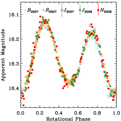
Figure 1.— Four-color lightcurve of Haumea. Symbols labelled 2008 correspond to the new $J$ and $H$ data presented here. Measurements from 2007 (Lacerda et al., 2008) are marked for direct comparison. The vertical axis corresponds to the $J_{2008}$ apparent magnitude. Data in other bands have been shifted using the mean colors (see text).

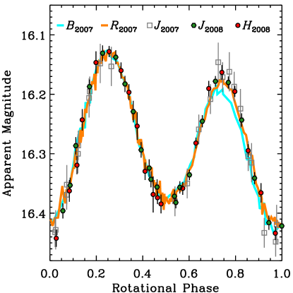
Figure 2.— Binned near-infrared lightcurve of Haumea. Here, sets of consecutive data points in Fig. 1 have been binned to reduce scatter. Green hexagons ($J$-band) and red circles ($H$-band) mark the mean rotational phase and magnitude of consecutive measurements (mostly sets of four). Measurements from 2007 (Lacerda et al., 2008) are marked for direct comparison: the green squares are $J$-band measurements, while the densely sampled $B$- and $R$-band data are plotted as thick cyan and orange lines. The vertical axis corresponds to the $J_{2008}$ apparent magnitude. Data in other bands have been shifted using the mean colors (see text).

The new data record just over one full rotation of Haumea. Figure 1 combines previously published $B$ and $R$ data (Lacerda et al., 2008) with the new $J$ and $H$ data and shows that all four filters exhibit very similar variability with a combined total range $\Delta m=0.30\pm 0.02$ mag. As described in §2, to improve the signal-to-noise ratios of the $J$ and $H$ data, we binned sets of measurements taken back-to-back (usually sets of four); the resulting lightcurve is shown in Fig. 2. There, the previously identified dark, red spot (DRS; Lacerda et al., 2008) on the surface of Haumea is clearly apparent at rotational phases close to $\phi=0.8$ in the $B$ and $R$ curves. The near-infrared data generally follow the $R$-band data but show a slight visible/near-infrared reddening which coincides with the DRS.

The differences between the individual lightcurves in Figs. 1 and 2 are small. To highlight color variations on Haumea, we plot in Fig. 3 all possible combinations of visible-to-near-infrared color curves. The curves are calculated by interpolating the better-sampled $B$ and $R$ data to the binned $J$ and $H$ rotational phases (Fig. 2) and subtracting. The error bars are dominated by the uncertainties in the near-infrared measurements, which are added quadratically to the mean $B$ or $R$ errors. When taken separately, the color curves in Fig. 3 appear to differ only marginally from a rotationally constant value. However, the color $B$$-$$H$, and arguably $B$$-$$J$, $R$$-$$H$, and $J$$-$$H$, show visible reddening humps for rotational phases close to where the DRS was found to lie ($\phi\sim 0.8$). To locate and quantify color variability features in the curves in Fig. 3 we employ a running Gaussian probability test. In this test we consider a moving rotational phase window and calculate the quantity

$$G=\frac{\sum_{i=1}^{N}(c_{i}-c_{0})/e_{i}}{\sqrt{N}}$$ (1)

for the points that fall within the window. In Eq. (1), $N$ is the number of points within the window, $c_{i}$ and $e_{i}$ are the color values and respective error bars of those points, and $c_{0}$ is the median color of all points (dotted horizontal lines in Fig. 3). We then move the window along each color curve in rotational phase steps of 0.05 to obtain a running-$G$ value. Equation (1) represents a Gaussian deviate with zero mean and unity standard deviation and can thus be converted to a Gaussian probability, $p(G)$, assuming that the points are normally distributed around the median. The probability $p(G)$ is sensitive to unlikely sequences of deviant points, all on one side of the median. Figure 4 shows the test results for each of the color curves using a window size $\Delta\phi=0.25$ (see discussion below). The Figure shows that the $B$$-$$H$ curve has a significant ($\sim$4$\sigma$) non-random feature close to $\phi=0.8$. The test also detects weaker (2.8$\sigma$ and 2.5$\sigma$) features in the $B$$-$$J$ and $R$$-$$H$ curves close to $\phi=0.8$.

Figure 3.— Visible and near-infrared color curves of Haumea. Each curve represents deviations from the respective rotationally-medianed mean color (from bottom up, $B$$-$$J=1.856\pm 0.012$ mag, $B$$-$$H=1.799\pm 0.021$ mag, $R$$-$$J=0.885\pm 0.012$ mag, $R$$-$$H=0.828\pm 0.016$ mag, and $J$$-$$H=-0.057\pm 0.016$ mag) and is vertically shifted by 0.1 mag for clarity. Slight reddening bumps are observable in $B$$-$$H$, $B$$-$$J$, and possibly in $R$$-$$H$ and $J$$-$$H$.

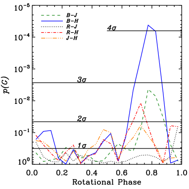
Figure 4.— Running Gaussian probability for each of the color curves in Fig. 3. Unlikely sequences of points all above or below the median colors (horizontal, dotted lines in Fig. 3) will be visible as peaks in this Figure. The color curve $B$$-$$H$ color shows a significant peak at rotational phase $\phi\sim 0.8$. Curves $B$$-$$J$ and $R$$-$$H$ show smaller but noticeable features at the same rotational phase.

Figure 5.— Running Gaussian probability for the $B$$-$$H$ color curve for four window sizes, $\Delta\phi=0.20$, 0.25, 0.33, and 0.50. The running probability $p(G)$ is calculated in a window of width $\Delta\phi$ which is evaluated in rotational phase steps of 0.05. The differences are minimal for window sizes $0.20\leq\Delta\phi\leq 0.33$. For the largest window size $\Delta\phi=0.50$ the probability begins to appear dilluted. See text for details.

The size of the rotational phase window $\Delta\phi$ is physically motivated by the fraction of the surface of Haumea that is visible at any given instant. In that sense, it should not be larger than $\Delta\phi=0.5$. Moreover, although half the surface is visible, projection effects in the limb region will make the effective visible area smaller, by possibly another factor 2. In Fig. 5 we illustrate the effect of the window size by replotting the running $p(G)$ for color curve $B$$-$$H$ using four window sizes, $\Delta\phi=0.20$, 0.25, 0.33, and 0.50. As expected, $p(G)$ does not differ much for windows $0.20\leq\Delta\phi\leq 0.33$. For the largest window size $\Delta\phi=0.50$ the probability begins to appear dilluted, but even then the test succeeds in locating the feature at $\phi=0.8$.

The near-infrared measurements presented here are considerably less numerous than the the optical data that were used to identify the DRS in $B$$-$$R$ (Lacerda et al., 2008). Also, the $J$ and $H$ measurements may show systematic correlations because they were measured on the same night using the same telescope. Nevertheless, the observed changes in $B$ and $R$ relative to $J$ and $H$ do not suffer from this effect and are likely to be real. A visible/near-infrared reddening was already observed in our 2007 data (see $J_{2007}$ points in Fig. 1) adding confidence to our conclusions. The results presented above suggest that the region close to the DRS is also spectrally anomalous in the visible-to-near-infrared wavelength range with respect to the average surface of Haumea.

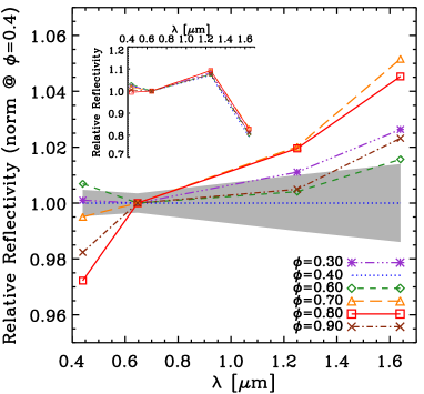
Figure 6.— Normalized reflectivity vs. wavelength for different rotational phases. The reflectivities were computed from the broadband colors by subtracting the colors of the Sun ($B-R=0.996$, $R-J=0.797$, $J-H=0.258$; cf. Holmberg et al., 2006). All curves were normalized at the $R$-band, and divided by the curve at rotational phase $\phi=0.4$, for clarity. The inset shows the reflectivities prior to dividing by the $\phi=0.4$ curve. The shaded polygon represents the uncertainty propagated from errors of measurement.

In Fig. 6 we combine our four-band data to produce reflectivity vs. wavelength curves at different rotational phases. We focus on the DRS region and plot curves at $\phi=0.3$ and $\phi=0.4$ as illustrative of the mean Haumea surface. We employed interpolation to calculate color indices at the given rotational phases, which were subsequently converted to reflectivities relative to the $R$-band. To enhance the subtle differences with rotation we normalize all curves by that at $\phi=0.4$; an inset in Fig. 6 shows the reflectivities before normalization. Figure 6 shows that relative to the majority of the surface of Haumea the region near $\phi=0.7$ displays an enhanced $H$-band reflectivity which, close to $\phi=0.8$, is accompanied by a depressed $B$-band reflectivity. Close to $\phi=0.9$, $B$ remains depressed, while $H$ is restored to average values. We note that this variation is consistent with the results shown in Fig. 4. To summarize, the DRS region is both fainter in $B$ and brighter in $H$ than the rest of Haumea.

The presence of a blue absorber on the DRS could explain the fainter $B$ reflectance. A recent $U$- and $B$-band photometric study of KBOs (Jewitt et al., 2007) suggests that objects in the classical population (objects in quasi-circular orbits between the 2:1 and the 3:2 mean-motion resonance with Neptune) lack significant blue absorption. As discussed by those authors, $B$-band absorption in main-belt asteroids is generally linked with the presence of phyllosilicates and other hydrated minerals (see also Gaffey & McCord, 1978; Feierberg et al., 1985) and is a characteristic feature in the spectra of C and G-type asteroids (Tholen & Barucci, 1989). How likely is it that Haumea has hydrated minerals on its surface? Although Haumea is located in the classical population as defined above, it is atypical in its water-ice dominated surface spectrum and its high bulk density (2.5 times water). These two properties suggest a differentiated body with significant rocky content. Furthermore, KBOs (mainly the larger ones) have possibly sustained liquid water in their interiors due to radiogenic heating (Merk & Prialnik, 2006). It would therefore be unremarkable to find trace amounts of hydrated minerals on Haumea. In fact, fits to the near-infrared spectrum of Haumea are slightly improved by the addition of phyllosilicates such as kaolinite and montmorillonite (Trujillo et al., 2007). Ultraviolet spectra of Haumea at different rotational phases are needed to further constrain the character of the blue absorption close to the DRS.

Our $J$ and $H$ photometry suggests that the 1.5 $\mu$m water-ice band is weaker (less deep) close to the DRS. In contrast, Lacerda et al. (2008) found marginal evidence that the 1.5 $\mu$m band is deeper close to the DRS. One difference between the two measurements is that while here we use $J$ vs. $H$, Lacerda et al. (2008) used $J$ vs. the “CH4_s” filter to assess possible variations in the water-ice band. The latter filter has a bandpass (center 1.60 $\mu$m, FWHM 0.11 $\mu$m) between the 1.5 $\mu$m and the 1.65 $\mu$m band diagnostic of crystalline water-ice and is thus affected by the degree of crystallinity of the ice. The two measurements can be reconciled if the DRS material has an overall less deep 1.5 $\mu$m water-ice band but a larger relative abundance of crystalline water ice. We simulated this scenario using synthetic reflectance spectra [calculated using published optical constants for crystalline water ice (Grundy & Schmitt, 1998) and a Hapke model with the best fit parameters for Haumea (Trujillo et al., 2007)]. By convolving two model spectra, one for $T=30$ K and one for $T=140$ K (to simulate a weaker crystalline band), with the $J$, $H$, and CH4_s bandpasses we found an effect similar to what is observed. The 30 K spectrum, taken to represent the DRS material, shows a $\sim$3% higher $H$-to-$J$ flux ratio, but a $\sim$4% lower CH_s-to-$J$ flux ratio than the 140 K spectrum. However, this possibility is not unique and time-resolved $H$-band spectra are required to test this scenario.

3.2. Phase Function

Atmosphereless solar system bodies exhibit a linear increase in brightness with decreasing phase angle. At small angles ($\alpha<0.01$ to 1 deg), this phase function becomes non-linear causing a sharp magnitude peak. The main physical mechanisms thought to be responsible for this opposition brightening effect are shadowing and coherent backscattering. In simple terms, shadowing occurs because although a photon can always scatter back in the direction from which it hit the surface, other directions may be blocked. The implication is that back-illuminated ($\alpha\sim 0$°) objects do not shadow their own surfaces and appear brighter. The brightening due to coherent backscattering results from the constructive interference of photons that scatter in the backwards direction from pairs of surface particles (or of features within a particle; Nelson et al., 2000). The constructive interfence decreases rapidly with increasing phase angle. Generally, it is believed that shadowing regulates the decrease in brightness with phase angle from a few up to tens of degrees, while coherent backscattering mainly produces the near-zero phase angle spike (French et al., 2007).

Figure 7.— Phase coefficient of Haumea as a function of wavelength. From left to right, points mark the central wavelength of the $B$, $V$, $I$, and $J$ bands. Our measurement of the $J$-band phase coefficient, $\beta_{J}=0.16\pm 0.04\,$mag deg^-1 is highlighted. The remaining three points are taken from Rabinowitz et al. (2006). A linear best-fit (slope 0.09 and 1 $\mu$m value 0.14) is overplotted as a dotted line.

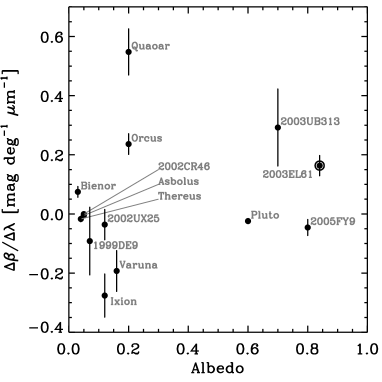
Figure 8.— Slope of the $\beta(\lambda)$ relation versus approximate geometric albedo for a number of KBOs and Centaurs. No clear relation exists between the two quantities.

The relative importance of shadowing and coherent backscattering on a given surface is difficult to assess. An early prediction by Hapke (1993) was that the angular width of the exponential brightness peak should vary linearly with wavelength in the case of coherent backscattering, given its interference nature. Shadowing, on the other hand, should be acromatic. However, more recent work has shown that the wavelength dependence of coherent backscattering can be very weak (Nelson et al., 2000). Thus, while a strong wavelength dependence is usually attributable to coherent backscattering, a weak wavelength dependence may be explained by either mechanism. It was also expected that higher albedo surfaces should be less affected by shadowing because more multiply scattered photons will reach the observer even from shadowed surface regions (Nelson et al., 1998). Coherent backscattering is a multiple-scattering process that thrives on highly reflective surfaces. Subsequent studies have shown that low albedo surfaces can also display strong coherent backscattering at very low phase angles (Hapke et al., 1998). Finally, while both effects cause a brightening towards opposition, only coherent backscattering has an effect on the polarization properties of light scattered from those objects: it favors the electric field component parallel to the scattering plane and thus gives rise to partially linearly polarized light (Boehnhardt et al., 2004; Bagnulo et al., 2006). With the currently available instruments, useful polarization measurements can only be obtained on the brightest KBOs.

Our July 2007 $J$-band lightcurve data (Lacerda et al., 2008) and the April 2008 data presented here together show that Haumea appears brighter in the latter dataset. After calculating the time-medianed apparent magnitudes, and correcting them to unit helio- and geocentric distances ($R$ and $\Delta$) using $m_{J}(1,1,\alpha)=m_{J}-5\log(R\Delta)$, a difference of 0.096 magnitudes remains between the datasets, which we attribute to the different phase angles ($\alpha_{2007}=1.13$ deg and $\alpha_{2008}=0.55$ deg) at the two epochs. Assuming a phase function of the form $m_{J}(\alpha)=m_{J}(1,1,0)+\beta_{J}\alpha$, we derive a slope $\beta_{J}=0.16\pm 0.04$ mag deg^-1. The uncertainty in $\beta_{J}$ was calculated by interpolating the 2008 $J$ lightcurve to the rotational phases of the 2007 $J$ lightcurve (both corrected to $R=\Delta=1$ AU) and calculating the standard deviation of the difference.

In Fig. 7 we plot the phase coefficient $\beta$ versus the central wavelengths of the filters $B$, $V$, $I$, and $J$. The visible $\beta_{B,V,I}$ values are taken from Rabinowitz et al. (2006) where they are measured in the phase range $0.5<\alpha<1.0$ deg. A linear fit to the relation is overplotted as a dotted line showing that $\beta_{\lambda}$ increases with $\lambda$. The fit has a slope $\Delta\beta/\Delta\lambda=0.09\pm 0.03$ mag deg^-1 $\mu$m^-1 and a 1 $\mu$m value $\beta_{1\mu\mathrm{m}}=0.14\pm 0.02$ mag deg^-1. Using a $\chi^{2}$ test we are only able to reject a constant $\beta_{\lambda}$ at the 2$\sigma$ level. However, the monotonic increase of $\beta_{\lambda}$ with wavelength plus the high albedo ($p_{V}>0.6$, Rabinowitz et al., 2006) of Haumea both suggest that coherent backscattering is dominant in the range of phase angles observed.

Small icy bodies in the solar system show very diverse phase function vs. wavelength behaviors (Rabinowitz et al., 2007). Most KBOs for which the phase curve has been measured in more than one band show steeper slopes towards longer wavelengths. We show here that in the case of Haumea this behavior extends into the near-infrared. The Centaurs (Rabinowitz et al., 2007) and the Uranian satellites (Karkoschka, 2001) show little variation in the phase curve with wavelength for $\alpha<3$ to 6 deg, suggesting that shadowing is dominant over coherent backscattering. Other objects show opposite or even non-monotonic relations between phase function slope and wavelength. For instance, some type of terrain on the Jovian moon Europa have phase functions that vary non-monotonically with wavelength (Helfenstein et al., 1998), while Pluto’s phase function has a weak wavelength dependence opposite to that seen in Haumea, from $\beta_{B}=0.037\pm 0.001$ mag deg^-1 to $\beta_{R}=0.032\pm 0.001$ mag deg^-1 (Buratti et al., 2003).

In Fig. 8 we plot the slope of the $\beta_{\lambda}$ vs. $\lambda$ relation against approximate geometric albedo for a number of KBOs and Centaurs. The values $\Delta\beta/\Delta\lambda$ were obtained from linear fits to the phase slope measurements in three bands by Rabinowitz et al. (2007). The scatter in Fig. 8 is substantial and no clear relation is evident between albedo and the wavelength dependance of the phase function. As a result, the interpretation of these results in terms of physical properties of the surface is problematic. The photometric (and polarimetric) phase functions depend in a non-trivial way on the size and spatial arrangement of surface regolith particles, as well as on their composition. Besides, the phase functions of KBOs can only be measured in a narrow range of phase angles (currently $0.5<\alpha<1.2$ deg in the case of Haumea) making it difficult to recognize the presence or width of narrow opposition peaks. Nevertheless, further evidence that coherent backscattering is responsible for the observed linearity between $\beta$ and $\lambda$ can be sought using polarization measurements of the surface of Haumea.

3.3. Satellite

We stacked our $\sim$70 frames in each filter to increase the signal-to-noise ratio of any real features around Haumea and so attempt to detect the satellites. In the stacked frames, we used a field star as representative of the point-spread function (PSF), scaled it to the brightest pixel of Haumea and subtracted it from the KBO. The result is shown in Figs. 9 and 10, where the original image, the PSF, and the subtracted image are plotted; one satellite, Hi’iaka, is clearly visible through both filters. We measure a Hi’iaka-Haumea separation $d=0.872\pm 0.002$″ ($\mathrm{PA}=184.67\pm 0.13$ deg), and flux ratios (with respect to Haumea) of $0.088\pm 0.001$ and $0.064\pm 0.002$ in $J$ and $H$, respectively. The mean UT of the frame stack is 2008 Apr 15.23134. We do not detect any other sources in the vicinity of Haumea, although we are sensitive to objects as faint as 0.11$\times$ the $J$-band (and 0.21$\times$ the $H$-band) flux of Hi’iaka. At the time of observation, the fainter, inner satellite Namaka was within 0.2″ of Haumea (Ragozzine, private comm.), which explains why it is invisible in our data. Given its fractional brightness ($\sim$1%) with respect to Haumea, Namaka has negligible contribution to the near-infrared photometry presented here.

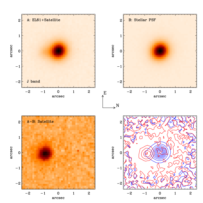
Figure 9.— Top left: Stack of $\sim 70$ $J$-band frames of Haumea. The satellite Hi’iaka is discernible to the left of Haumea. Top right: Stellar PSF built from a stack of $\sim 70$ $J$-band frames of a star in the Haumea field. Bottom left: Image of Hi’iaka obtained by subtracting the top right image from the top left one. Bottom right: Contours of Haumea and Hi’iaka (blue) overplotted on contours of the satellite Hi’iaka alone (red) to show the relative position.

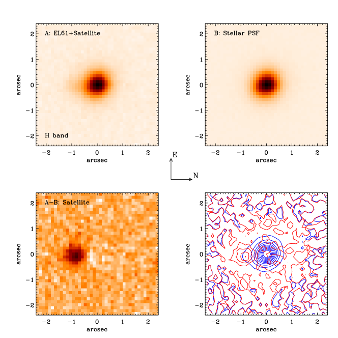
Figure 10.— Same as Fig. 9 for $H$-band data.

Haumea has a color index $J\!-\!H=-0.057\pm 0.016$ mag (see Fig. 3 and Table 6). Our photometry of Hi’iaka relative to Haumea implies a color $J\!-\!H=-0.399\pm 0.034$ mag for the former. This color index is unusually blue, but consistent with the observation that the 1.5 $\mu$m band is deeper for Hi’iaka than for Haumea (Takato et al., 2006; Barkume et al., 2006). Table 6 lists the derived colors of Haumea and Hi’iaka. A sample of $J\!-\!H$ colors of 40 KBOs and Centaurs found in the literature (Delsanti et al., 2006) shows a pronounced clustering around $J\!-\!H=0.4$ mag with a dispersion of $\sim$0.2 mag. The two significant outliers are KBOs (19308) 1996 TO₆₆ ($J\!-\!H=-0.21\pm 0.17$ mag) and (24835) 1995 SM₅₅ ($J\!-\!H=-0.49\pm 0.06$ mag) which both possess near-infrared spectra consistent with water-ice absorption (Brown et al., 1999; Barkume et al., 2008).

The $J\!-\!H$ colors of Haumea and Hi’iaka are significantly ($>$9$\sigma$) different. Given the current best estimates for the mass and orbit of Hi’iaka, particles collisionally ejected (ejection velocities 10 to 200 m s^-1) from its surface will likely reach Haumea only on hyperbolic orbits (Stern, 2008). The escape speed from the surface of Hi’iaka (near 130 m s^-1, assuming water-ice density) rivals the escape speed from the Haumea system at the orbit of Hi’iaka ($\sim$120 m s^-1), meaning that only hyperbolic mass exchange is possible. The same cannot be said about Namaka which is both smaller and deeper into the potential well of the satellite system. It is therefore more likely that Haumea is polluted by ejecta from Namaka than from Hi’iaka. Whether this means that the $J\!-\!H$ color of Namaka is closer to that of Haumea remains to be seen.

4. Summary

From time-resolved, near-infared photometry of Kuiper belt object Haumea we find the following

• The near-infrared peak-to-peak photometric range is $\Delta m_{R}$ = 0.30$\pm$0.02 mag. The new data reveal slight visible/near-infrared color variations on Haumea, which are spatially correlated with a previously identified surface region, redder in $B\!-\!R$ and darker than the mean surface. We find that near this region Haumea displays an enhanced $H$-band reflectance accompanied by $B$-band absorption relative to elsewhere on the surface. Time-resolved spectra are needed to learn more about the physicochemical properties of this anomalous region.

• The rotationally medianed visible and near-infrared colors of Haumea are $R\!-\!J=0.885\pm 0.012$ mag and $J\!-\!H=-0.057\pm 0.016$ mag.

• We detect Hi’iaka, Haumea’s brightest satellite, in both $J$ and $H$ and measure its color $J\!-\!H=-0.399\pm 0.034$ mag. The $J\!-\!H$ color difference between Hi’iaka and Haumea is significant ($>$9$\sigma$). This suggests that either the transfer of surface ejecta between the two is negligible, or that their surface colors are not controlled by ejecta transfer. Ejecta transfer between Haumea and the inner satellite Namaka is neither ruled out nor substantiated by our data but is more likely given the configuration of the system.

• The slope of the $J$-band phase function in the range $0.55\leq\alpha(\mathrm{deg})\leq 1.14$ is $\beta_{J}=0.16\pm 0.04$ mag deg^-1. Combining this measurement with slopes obtained in three other visible wavelengths we find that the slope of Haumea’s phase function varies monotonically with wavelength. The slope of the relation is $\Delta\beta/\Delta\lambda\sim 0.09$ mag deg^-1 $\mu$m^-1 and $\beta_{1\mu\mathrm{m}}\sim 0.14$ mag deg^-1. This finding confirms previous inferences that coherent backscattering is the main cause of opposition brightening for Haumea.

References

- Bagnulo et al. (2006) Bagnulo, S., Boehnhardt, H., Muinonen, K., Kolokolova, L., Belskaya, I., & Barucci, M. A. 2006, A&A, 450, 1239
- Barkume et al. (2006) Barkume, K. M., Brown, M. E., & Schaller, E. L. 2006, ApJ, 640, L87
- Barkume et al. (2008) —. 2008, AJ, 135, 55
- Boehnhardt et al. (2004) Boehnhardt, H., Bagnulo, S., Muinonen, K., Barucci, M. A., Kolokolova, L., Dotto, E., & Tozzi, G. P. 2004, A&A, 415, L21
- Brown et al. (2007) Brown, M. E., Barkume, K. M., Ragozzine, D., & Schaller, E. L. 2007, Nature, 446, 294
- Brown et al. (2005) Brown, M. E., Trujillo, C. A., & Rabinowitz, D. L. 2005, ApJ, 635, L97
- Brown et al. (2006) Brown, M. E., et al. 2006, ApJ, 639, L43
- Brown et al. (1999) Brown, R. H., Cruikshank, D. P., & Pendleton, Y. 1999, ApJ, 519, L101
- Buratti et al. (2003) Buratti, B. J., et al. 2003, Icarus, 162, 171
- Cruikshank et al. (1976) Cruikshank, D. P., Pilcher, C. B., & Morrison, D. 1976, Science, 194, 835
- Delsanti et al. (2006) Delsanti, A., Peixinho, N., Boehnhardt, H., Barucci, A., Merlin, F., Doressoundiram, A., & Davies, J. K. 2006, AJ, 131, 1851
- Feierberg et al. (1985) Feierberg, M. A., Lebofsky, L. A., & Tholen, D. J. 1985, Icarus, 63, 183
- French et al. (2007) French, R. G., Verbiscer, A., Salo, H., McGhee, C., & Dones, L. 2007, PASP, 119, 623
- Gaffey & McCord (1978) Gaffey, M. J., & McCord, T. B. 1978, Space Science Reviews, 21, 555
- Grundy & Schmitt (1998) Grundy, W. M., & Schmitt, B. 1998, J. Geophys. Res., 103, 25809
- Hapke (1993) Hapke, B. 1993, Theory of reflectance and emittance spectroscopy (Topics in Remote Sensing, Cambridge, UK: Cambridge University Press, —c1993)
- Hapke et al. (1998) Hapke, B., Nelson, R., & Smythe, W. 1998, Icarus, 133, 89
- Hawarden et al. (2001) Hawarden, T. G., Leggett, S. K., Letawsky, M. B., Ballantyne, D. R., & Casali, M. M. 2001, MNRAS, 325, 563
- Helfenstein et al. (1998) Helfenstein, P., et al. 1998, Icarus, 135, 41
- Holmberg et al. (2006) Holmberg, J., Flynn, C., & Portinari, L. 2006, MNRAS, 367, 449
- Jewitt et al. (2007) Jewitt, D., Peixinho, N., & Hsieh, H. H. 2007, AJ, 134, 2046
- Karkoschka (2001) Karkoschka, E. 2001, Icarus, 151, 51
- Lacerda et al. (2008) Lacerda, P., Jewitt, D., & Peixinho, N. 2008, AJ, 135, 1749
- Lacerda & Jewitt (2007) Lacerda, P., & Jewitt, D. C. 2007, AJ, 133, 1393
- Licandro et al. (2006) Licandro, J., Pinilla-Alonso, N., Pedani, M., Oliva, E., Tozzi, G. P., & Grundy, W. M. 2006, A&A, 445, L35
- Malhotra (1995) Malhotra, R. 1995, AJ, 110, 420
- Merk & Prialnik (2006) Merk, R., & Prialnik, D. 2006, Icarus, 183, 283
- Nelson et al. (1998) Nelson, R. M., Hapke, B. W., Smythe, W. D., & Horn, L. J. 1998, Icarus, 131, 223
- Nelson et al. (2000) Nelson, R. M., Hapke, B. W., Smythe, W. D., & Spilker, L. J. 2000, Icarus, 147, 545
- Rabinowitz et al. (2006) Rabinowitz, D. L., Barkume, K., Brown, M. E., Roe, H., Schwartz, M., Tourtellotte, S., & Trujillo, C. 2006, ApJ, 639, 1238
- Rabinowitz et al. (2007) Rabinowitz, D. L., Schaefer, B. E., & Tourtellotte, S. W. 2007, AJ, 133, 26
- Ragozzine & Brown (2007) Ragozzine, D., & Brown, M. E. 2007, AJ, 134, 2160
- Stern (2008) Stern, S. A. 2008, ArXiv e-prints, 805
- Takato et al. (2006) Takato, N., Terada, H., & Tae-Soo, P. 2006, Oral communication
- Tegler et al. (2007) Tegler, S. C., Grundy, W. M., Romanishin, W., Consolmagno, G. J., Mogren, K., & Vilas, F. 2007, AJ, 133, 526
- Tholen & Barucci (1989) Tholen, D. J., & Barucci, M. A. 1989, in Asteroids II, ed. R. P. Binzel, T. Gehrels, & M. S. Matthews, 298–315
- Tokoku et al. (2003) Tokoku, C., et al. 2003, in Instrument Design and Performance for Optical/Infrared Ground-based Telescopes., ed. M. Iye & A. F. M. Moorwood, Vol. 4841, 1625–1633
- Trujillo et al. (2007) Trujillo, C. A., Brown, M. E., Barkume, K. M., Schaller, E. L., & Rabinowitz, D. L. 2007, ApJ, 655, 1172