Adhesion-induced lateral phase separation of multi-component membranes: the effect of repellers and confinement

Abstract

We present a theoretical study for adhesion-induced lateral phase separation for a membrane with short stickers, long stickers and repellers confined between two hard walls. The effects of confinement and repellers on lateral phase separation are investigated. We find that the critical potential depth of the stickers for lateral phase separation increases as the distance between the hard walls decreases. This suggests confinement-induced or force-induced mixing of stickers. We also find that stiff repellers tend to enhance, while soft repellers tend to suppress adhesion-induced lateral phase separation.

1 Introduction

Biological membranes are lipid bilayers with different types of embedded or absorbed macromolecules. They serve a number of general functions in our cells and tissues [1, 2]. Because of its biological importance, the physics of membrane adhesion has received considerable attention both theoretically and experimentally [3, 4, 5, 6, 7, 8, 9, 10]. For instance, helper T cells mediate immune responses by adhering to antigen-presenting cells (APCs) which exhibit foreign peptide fragments on their surface. [11]. The APC membranes contain the ligands MHCp and ICAM-1 while the T cells contain the receptors TCR and LFA-1. The experiments [11] show the formation of domains into shorter TCR/MHCp receptor-ligand complexes and the longer LFA-1/ICAM-1 receptor-ligand complexes. The dynamics of adhesion-induced phase separation has been studied theoretically [12, 13, 14]. For example, the Monte Carlo study by Weikl and Lipowsky [14] shows that the height difference between different junctions causes a lateral phase separation, and the formation of target-like immunological synapse is assisted by the motion of cytoskeleton.

The equilibrium studies of adhesion-induced phase separation of multi-component membranes are also important for a complete understanding of the physics of membrane adhesion. For instance, in recent articles [15, 16], the general case of two membranes binding to each other with two types of stickers is considered and the equilibrium phase behavior of such a system is studied at the mean field and Gaussian level by including the effects of sticker flexibility difference, sticker height difference and thermally activated membrane height fluctuations. More recently, Mesfin $et$ $al.$ [17] presented a theoretical study that characterized the phase diagram and the scaling laws for the critical potential depth of unbinding and lateral phase separation. These studies show that membranes are unbound for small potential depths and bound for large potential depths. In the bound state, the length mismatch leads to a membrane-mediated repulsion between stickers of different lengths and this leads to lateral phase separation depending the concentrations and strengths of the receptor-ligand bonds. Furthermore, the flexibilities of the stickers play non-trivial roles in the location of phase boundaries.

Most of these recent works deal with membranes with one or two types of stickers. However, biological membranes usually contain glycoproteins which are repulsive to another membrane or tissue, i.e., they act as repellers. This important fact motivates us to study adhesion-induced lateral phase separation of membranes with short stickers, long stickers and repellers. Another important but unexplored issue on adhesion-induced lateral phase separation in biomembranes is the effect of external pressure or confinement on the phase diagram. For example, cell adhesions often occur in the presence of external force field due to external flow, or the external force may be a result of the occurrence of cell adhesions in highly confined geometry during the development of multicellular organisms. To study the effect of repellers and confinement on adhesion-induced lateral phase separation, in this article we first consider a membrane with short stickers and long stickers which are in contact with another planer surface (substrate) in the absence of repellers. The membrane and the substrate are confined between two hard walls. We find that the critical binding energies of the stickers for lateral phase separation increase as the distance between the hard walls decreases due to the steric repulsion of the membrane with the hard walls. Then the effect of repellers are considered and we find that stiff repellers tend to enhance phase separation, while soft repellers tend to suppress phase separation. Our study has revealed the possibility to manipulating the lateral distribution of stickers in future experiments.

This paper is organized as follows: In section II we present the model of membranes with short stickers, long stickers and repellers. By tracing out sticker and repeller degrees of freedom, we get membranes that interact with an effective double-well potential. The adhesion-induced lateral phase separation in the presence of stickers and repellers is studied by mean field theory and Monte Carlo simulations in section III. First we consider membranes with short and long stickers. We then consider membranes with short, long stickers and repellers. Section IV is the summary and conclusion.

2 The model

We consider a tensionless non-homogenous multi-component membrane with short and long receptor-ligand bonds that interacts with a substrate as shown in Fig. 1. Let us denote the short and long receptor-ligand bonds as short and long stickers, respectively. In our model, the membrane is discretized into a two dimensional square lattice with lattice constant $a$ [8, 17]. The lattice constant $a$ is chosen to be $a=6{\rm nm}$, the smallest length scale for membrane continuum elasticity theory to be valid. The separation field $l\geq 0$ describes the vertical distance between the membrane and the substrate. An additional field $n_{i}=0,\ 1,\ 2$, or $3$ denotes the occupation state of the $i$th site. $n_{i}=0$ indicates the absence of stickers and repellers at lattice site $i$ while $n_{i}=1(2)$ denote the presence of a type-1(2) sticker at lattice site $i$; $n_{i}=3$ denotes the presence of a repeller at a site $i$.

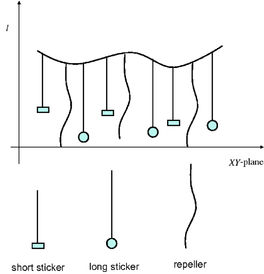
Figure 1: Schematic figure for a membrane with short stickers, long stickers and repellers close to a substrate. The local separation field is $l$.

The grand canonical Hamiltonian of the system under consideration is given by

$$H[l,n] = H_{el}[l]+\sum_{i}\delta_{1,n_{i}}(V_{1}(l_{i})-\mu_{1})+$$ (1)

$$\sum_{i}\delta_{2,n_{i}}(V_{2}(l_{i})-\mu_{2})+\sum_{i}\delta_{3,n_{i}}(V_{3}(l_{i})-\mu_{3})$$

here $H_{el}[l]=\sum_{i}{\kappa\over 2a^{2}}(\Delta_{d}l_{i})^{2}$ denotes the discretized bending energy of the membrane with bending rigidity $\kappa$. Typically, $\kappa=10-20{\rm k_{B}T}$. The discretized Laplacian $\Delta_{d}$ is given by $\Delta_{d}l_{i}=l_{i1}+l_{i2}+l_{i3}+l_{i4}-4l_{i}$ where $l_{i1}$ to $l_{i4}$ are the four nearest-neighbor membrane separation fields of the membrane patch $i$. The second and third terms on the right hand side of Eq. (1) are interaction potentials between the stickers and the substrate. $\mu_{1}$ and $\mu_{2}$ denote the chemical potentials of stickers 1 and 2, respectively. The parameters $V_{3}({\it l}_{i})$ and $\mu_{3}$ represent potentials and the chemical potentials of the repellers, respectively. We consider the following sticker potentials: for $\alpha=1,2$,

$$V_{\alpha}=\cases{U_{\alpha},&if $l_{\alpha}<l<l_{\alpha}+l_{we\alpha}$\cr 0,&otherwise\cr}$$ (2)

where $U_{1}$, $U_{2}$ are both negative and $l_{1}<l_{2}$. That is, type-1 stickers are shorter than type-2 stickers. The repulsive potential of the repellers is $V_{3}=U_{3}>0$ for $0<l<l_{3}$.

The equilibrium properties of the system can be obtained from the grand partition function $Z$,

$$Z=\prod_{i}\int_{0}^{\infty}dl_{i}\sum_{n_{i}=0}^{3}\exp\left[{-H[l,n]\over k_{B}T}\right].$$ (3)

Absorbing the Boltzmann constant $k_{B}$ into the temperature $T$ and tracing out the sticker degrees of freedom one gets

$$Z = \int_{0}^{\infty}\prod_{i}dl_{i}\exp\left[-H_{el}(l)\right]$$ (4)

$$\left[1+\exp\left[{-V_{1}(l_{i})+\mu_{1}\over T}\right]+\exp\left[{-V_{2}(l_{i})+\mu_{2}\over T}\right]+\exp\left[{-V_{3}(l_{i})+\mu_{3}\over T}\right]\right]$$

$$= \int_{0}^{\infty}dl_{i}\prod_{i}\exp\left[{-H_{el}(l)+\sum_{i}V^{eff}(l_{i})\over T}\right],$$

where the effective potential, $V^{eff}(l)$, is given by

$$V^{eff}=\cases{U_{ba},&for $0<l<l_{1}$;\cr U_{1}^{eff},&for $l_{1}<l<l_{1}+l_{we1}$;\cr U_{ba},&for $l_{1}+l_{we1}<l<l_{2};$\cr U_{2}^{eff},&for $l_{2}<l<l_{2}+l_{we2};$\cr U_{ba},&for $l_{we2}<l<l_{3};$\cr 0,&otherwise,\cr}$$ (5)

where

$$U_{1}^{eff}=-{T}\ln{\left[1+\exp[{-U_{1}+\mu_{1}\over T}]+\exp[{\mu_{2}\over T}]+\exp[{\mu_{3}\over T}]\over 1+\exp[{\mu_{1}\over T}]+\exp[{\mu_{2}\over T}]+\exp[{\mu_{3}\over T}]\right]},$$ (6)

$$U_{2}^{eff}=-{T}\ln{\left[1+\exp[{\mu_{1}\over T}]+\exp[{-U_{2}+\mu_{2}\over T}]+\exp[{\mu_{3}\over T}]\over 1+\exp[{\mu_{1}\over T}]+\exp[{\mu_{2}\over T}]+\exp[{\mu_{3}\over T}]\right]},$$ (7)

and

$$U_{ba}^{eff}=-{T}\ln{\left[1+\exp[{\mu_{1}\over T}]+\exp[{\mu_{2}\over T}]+\exp[{-U_{3}+\mu_{3}\over T}]\over 1+\exp[{\mu_{1}\over T}]+\exp[{\mu_{2}\over T}]+\exp[{\mu_{3}\over T}]\right]},$$ (8)

as shown in Fig. 2.

In the following section, the phase behavior of membranes under the effective potential given by Eq. (5) will be studied by mean field approximation and Monte Carlo simulations.

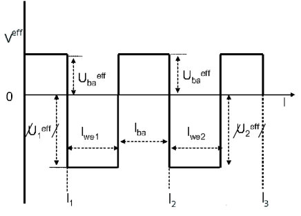
Figure 2: Schematic effective potential, $V^{eff}$ versus $l$. The potential has two square wells of depths $|{\bar{U}}_{1}^{eff}|$ and $|{\bar{U}}_{2}^{eff}|$ and one square barrier $U_{ba}^{eff}$.

3 Mean field theory and Monte Carlo simulation

It is convenient to introduce the rescaled separation field $z=(l/a)\sqrt{\kappa/T}$ and the rescaled effective potential ${\bar{V}}^{eff}=V^{eff}/T$. In equilibrium state the rescaled separation field $z$ fluctuates around its average value $z_{min}$. When the fluctuation is not very strong, mean field approximation can be applied to the discretized Laplacian such that $H_{l}[z]=\sum_{i}(4[z_{min}-z_{i}])^{2}$. In this approximation $z_{i}$ at different sites are decoupled. Hence Eq. (4) becomes

$$Z = \left[\int_{0}^{\infty}dz\exp{[-8(z_{min}-z)^{2}-{\bar{V}}^{eff}(z)]}\right]^{N},$$ (9)

and the mean field free energy of the membrane is given by

$$G = -NT\ln[\left[\int_{0}^{\infty}dz[\exp[-8(z_{min}-z)^{2}-{\bar{V}}^{eff}(z)]]\right].$$ (10)

Minimizing the free energy (10) with respect to $z_{min}$ leads to the following self-consistence equation,

$$z_{min}={\int_{0}^{\infty}z\exp[-8(z_{min}-z)^{2}-{\bar{V}}^{eff}(z)]dz\over\int_{0}^{\infty}\exp[-8(z_{min}-z)^{2}-{\bar{V}}^{eff}(z)]dz}.$$ (11)

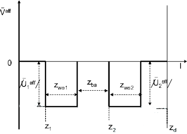
Figure 3: Model potential for membranes without repellers. The two wells are separated by a potential barrier of width $z_{ba}$. $z_{1}$ ($z_{d}$) is the distance between well one (well two) and the hard wall at $z=0$ ($z=z_{d}$). The effective potential $V^{eff}=\infty$ for $z\leq 0$ and $z\geq z_{d}$.

3.1 Membranes without repellers

Let us first consider a membrane without repellers, its effective potential is shown in Fig. 3. Since the critical phenomena for this system belongs to Ising universality class, for sufficiently strong potential depths the system is in two-phase state with two possible separations $z_{min1}$ and $z_{min2}$ [18]; for weak potential wells, the membrane can tunnel through the barrier between the wells and takes one average separation field $z_{min}$.

As an example, Figure 4 shows the relation between ${\bar{U}}_{2}^{eff}$ versus $z_{min}$ given by Eq. (11) for $z_{1}=0.1$, $z_{d}=1.2$, $z_{we1}=z_{we2}=0.2$ and $z_{ba}=0.4$. The effective binding energy of type-1 stickers $|{\bar{U}}_{1}^{eff}|$ is chosen to be $|{\bar{U}}_{1}^{eff}|=4$ for the upper curve and $|{\bar{U}}_{1}^{eff}|=|{\bar{U}}_{1c}^{eff}|=1.095$ for the lower curve. One finds that $z_{min}\rightarrow z_{1}+z_{we1}/2=0.2$ when $|{\bar{U}}_{2}^{eff}|\ll|{\bar{U}}_{1}^{eff}|$; $z_{min}$ increases as $|{\bar{U}}_{2}^{eff}|$ increases, and $z_{min}\rightarrow z_{2}+z_{we1}/2=0.8$ when $|{\bar{U}}_{2}^{eff}|\gg|{\bar{U}}_{1}^{eff}|$. However, when $|{\bar{U}}_{1}^{eff}|>|{\bar{U}}_{1c}^{eff}|$ there is a range of ${\bar{U}}_{2}^{eff}$ where $d|{\bar{U}}_{2}^{eff}|/dz_{min}$ becomes negative, this is unphysical. The physical equation of state in the two-phase state can be found from Maxwell’s equal-area construction, which also determines the phase boundary of the coexistence region for $|{\bar{U}}_{1}^{eff}|>|{\bar{U}}_{1c}^{eff}|$. The critical point (${\bar{U}}_{1C}^{eff}$, ${\bar{U}}_{2C}^{eff}$) is found by varying ${\bar{U}}_{1}^{eff}$ until $\partial U_{2}^{eff}/\partial z_{min}$ and $\partial^{2}U_{2}^{eff}/\partial^{2}z_{min}$ have common zero for given $z_{1}$, $z_{d}$, $z_{ba}$, $z_{we1}$ and $z_{we2}$.

Having discussed how to construct the phase diagram, we consider how confinement affects this adhesion-induced lateral phase separation. Figure 5a shows how ${\bar{U}}_{1c}^{eff}$ and ${\bar{U}}_{2c}^{eff}$ change as $z_{d}$ changes for $z_{1}=0.1$, $z_{ba}=0.4$, $z_{we1}=0.2$ and $z_{we2}=0.2$. The effect of confinement becomes important for $z_{d}\leq 1.5$, where $|{\bar{U}}_{1c}^{eff}|$ and $|{\bar{U}}_{2c}^{eff}|$ increase as $z_{d}$ decreases. This is because the entropic repulsion between the membrane and the hard wall located at $z_{d}$ increases as $z_{d}$ decreases, and the membrane is forced to tunnel through the barrier more often when $z_{d}$ decreases, thus strong confinement tend to suppress lateral phase separation. The phase diagrams for this system at several magnitudes of $z_{d}$ are shown in Fig.5b. It is clear that the critical points shift toward greater $|U_{1}^{eff}|$ and $|U_{2}^{eff}|$ as $z_{d}$ decreases. For $z_{d}=1$, the effective potential profile shown in Fig. 3 is symmetric and the phase coexistence line is on ${\bar{U}}_{1}^{eff}={\bar{U}}_{2}^{eff}$. When $z_{d}<1$, the phase coexistence line bends up; for $z_{d}>1$ the phase coexistence line shifts down in the vicinity of the critical point.

Figure 4: The effective potential depth $|{\bar{U}}_{2}^{eff}|$ versus $z_{min}$ for $z_{1}=0.1$, $z_{d}=1.2$, $z_{we1}=z_{we2}=0.2$ and $z_{ba}=0.4$. $|{\bar{U}}_{1}^{eff}|=4$ for the upper curve and $|{\bar{U}}_{1}^{eff}|=|{\bar{U}}_{1c}^{eff}|=1.095$ for the lower curve, respectively. The phase coexistence region for $|{\bar{U}}_{1}^{eff}|=4$ can be determined by Maxwell equal-area construction.

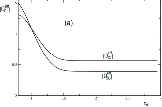
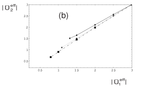
Figure 5: (a) The critical potential depths versus $z_{d}$ for $z_{1}=0.1$, $z_{ba}=0.4$, $z_{we1}=0.2$ and $z_{we2}=0.2$. When $z_{d}$ is small, $|{\bar{U}}_{1c}^{eff}|$ and $|{\bar{U}}_{2c}^{eff}|$ increases as $z_{d}$ decreases. (b) The phase boundaries for the system shown in Fig.5a. $z_{d}=0.9$ (top), $z_{d}=1$ (middle), and $z_{d}=1.2$ (bottom).

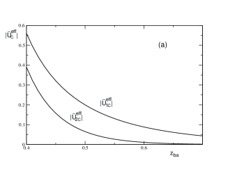
Figure 6: (a) The critical potential depths versus $z_{ba}$ for $z_{1}=0.1$, $z_{d}=6$, and $z_{we1}=z_{we2}=0.2$. $|{\bar{U}}_{1c}^{eff}|>|{\bar{U}}_{2c}^{eff}|$ for all $z_{ba}$ and both $|{\bar{U}}_{1c}^{eff}|$, $|{\bar{U}}_{2c}^{eff}|$ decrease as $z_{ba}$ increases. (b) The critical potential depths versus $z_{ba}$ for $z_{1}=0.1$, $z_{d}=6$, $z_{we1}=0.2$, and $z_{we2}=0.1$. $|{\bar{U}}_{2c}^{eff}|>|{\bar{U}}_{1c}^{eff}|$ for small $z_{ba}$, and $|{\bar{U}}_{1c}^{eff}|>|{\bar{U}}_{2c}^{eff}|$ for large $z_{ba}$.

Mean field theory is also convenient for studying how ${\bar{U}}_{1c}^{eff}$ and ${\bar{U}}_{2c}^{eff}$ vary as the length difference between the stickers changes. Fig.6a shows that, when the effect of confinement is negligible, as the length difference between short and long stickers increases, lateral phase separation occurs at lower $|{\bar{U}}_{1c}^{eff}|$ and $|{\bar{U}}_{2c}^{eff}|$, as one expected. Furthermore, for $z_{we1}=z_{we2}$, $|{\bar{U}}_{1c}^{eff}|>|{\bar{U}}_{2c}^{eff}|$ due to collisions between the membrane and the substrate. On the other hand, Fig.6b depicts that when $z_{we2}={1/2}z_{we1}$, $|{\bar{U}}_{2c}^{eff}|>|{\bar{U}}_{1c}^{eff}|$ when $z_{ba}$ is small due to the potential width difference. However, for large $z_{ba}$ the steric repulsion between a membrane in the second well and the substrate becomes unimportant, thus $|{\bar{U}}_{2c}^{eff}|<|{\bar{U}}_{1c}^{eff}|$ even though $z_{we2}<z_{we1}$. These results demonstrate that our mean field theory can be applied to analyze various physical effects on the adhesion-induced lateral phase separation. A more detailed study will likely require time-consuming large-scale numerical simulations.

To check whether the physics revealed by our simple mean-field analysis holds when fluctuations are taken into account, we compare the mean-field result with Monte Carlo simulation.

When $z_{d}$ and $z_{1}$ are both large, the effect of the walls is negligible. Hence when $z_{we1}=z_{we2}$, the membrane is effectively in a symmetric double-well potential [17]. The critical potential depths ${\bar{U}}_{1c}^{eff}={\bar{U}}_{2c}^{eff}={\bar{U}}^{eff}$. The location of the critical potential depth ${\bar{U}}_{c}^{eff}$ can be obtained by using Binder cumulant method [20]. The ${\bar{U}}^{eff}$ dependence of the Binder moments $C_{2}=\left\langle{\bar{z}}^{2}\right\rangle/\left\langle|{\bar{z}}|\right\rangle^{2}$ and $C_{4}=\left\langle{\bar{z}}^{4}\right\rangle/\left\langle{\bar{z}}^{2}\right\rangle^{2}$ is calculated for several system sizes and the critical point is located at the common intersection point of those curves due to the divergence of the correlation length at criticality. ${\bar{z}}={1\over N}\sum_{i=1}^{N}$ denotes the spatial average of the separation field while $\left\langle...\right\rangle$ represents thermal average. As an example, Figures 7a and 7b show $C_{2}$ and $C_{4}$ versus ${\bar{U}}^{eff}$ for $z_{1}=0.8$, $z_{d}=3.1$, $z_{2}=1.8$, $z_{we1}=z_{we2}=0.5$, and $z_{ba}=0.5$. The system size $L\times L$ in the simulations are $L=10$, $L=20$ and $L=30$. ${\bar{U}}_{c}^{eff}$ can be obtained from the common intersection point of $C_{2}$ and $C_{4}$ for different $L$.

The effect of confinement on lateral phase separation of membrane is important when $z_{d}$ and $z_{1}$ are small. In this case the walls affect the phase coexistence line and the critical potential depths. Thus the phase coexistence line and the critical potential depths in the simulations are determined by measuring the binding probability $P_{1}$ of the membrane in well-one, and the binding probability $P_{2}$ of the membrane in well-two. The simulation starts in the regime when both potential wells are deep and the membrane stays in well-two; then we decrease $|{\bar{U}}_{2}^{eff}|$, $P_{2}$ decreases continuously until the membrane switches from well-two to well-one. This discontinuous transition signals a first-order phase transition[21]. The location of the critical point can be determined by repeating the above procedure for systems with progressively smaller $|{\bar{U}}_{1}^{eff}|$. Below the critical point, the plot $P_{2}$ versus ${\bar{U}}_{2}^{eff}$ is continuous.

Figure 8 shows the phase diagram for $z_{1}=0.1$, $z_{ba}=0.4$, $z_{we1}=0.2$, and $z_{we2}=0.2$. For small $z_{d}$, the phase coexistence curve shifts up in the vicinity of the critical potential depth as membrane confined in well two feels higher entropic repulsion with the hard wall than membrane confined in well-one. For $z_{d}=1$, the effective potential is symmetric thus the phase coexistence line is at ${\bar{U}}_{1}^{eff}={\bar{U}}_{2}^{eff}$. For $z_{d}=1.2$ the phase boundary shifts down in the vicinity of the critical point. Although the critical points in the simulations are located at higher $|U_{1}^{eff}|$ and $|U_{2}^{eff}|$ than those in the mean field theory due to fluctuations, simulations also shown confinement enhanced phase separation. Thus, although mean field theory cannot provide accurate prediction for the critical points, it provides good prediction about the shape of phase boundary in $|U_{1}^{eff}|-|U_{2}^{eff}|$ plane and the entropic effect of confinement on the phase boundary.

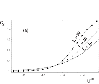
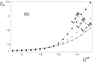
Figure 7: (a) The cummulant $C_{2}$ versus ${\bar{U}}^{eff}$ for $z_{1}=0.8$, $z_{d}=3.1$, $z_{2}=1.8$, $z_{we1}=z_{we2}=0.5$, and $z_{ba}=0.5$. The intersection point for $L=10$, $L=20$, and $L=30$ denotes the location of the critical potential depth ${\bar{U}}_{C}^{eff}$. (b) The cummulant $C_{4}$ versus ${\bar{U}}^{eff}$ for $z_{1}=0.8$, $z_{d}=3.1$, $z_{2}=1.8$, $z_{we1}=z_{we2}=0.5$ and $z_{ba}=0.5$.

Figure 8: Phase diagram in ${\bar{U}}_{1}^{eff}$ ${\bar{U}}_{2}^{eff}$ space constructed from Monte Carlo simulations for membranes without repellers. In the simulations $z_{1}=0.1$, $z_{ba}=0.4$, $z_{we1}=0.2$, and $z_{we2}=0.2$. $z_{d}=0.9$ (top), $z_{d}=1$ (middle), and $z_{d}=1.2$ (bottom).

3.2 Membranes with repellers

To study the effect of repellers on adhesion-induced lateral phase separation, first notice that adding repellers to a system means for given sticker species and densities ($U_{1}$, $\mu_{1}$, $U_{2}$, and $\mu_{2}$ are not changed), repellers with given $U_{3}$, $\mu_{3}$, and $l_{3}$ are added to the system. Therefore we need to see how effective potentials associated with the stickers change as repellers are added to the system.

For membranes containing repellers, the effective potential of the membrane takes the form

$${\bar{V}}^{eff}=\left\{\begin{array}[]{ll}\infty,&\mbox{for}~{}z<0,\\ {\bar{U}}_{ba}^{eff},&\mbox{for}~{}0<z<z_{1},\\ {\bar{U}}_{1}^{eff}\equiv[{\bar{U}}_{1}^{eff}]_{trans},&\mbox{for}~{}z_{1}<z<z_{1}+z_{we1},\\ {\bar{U}}^{eff}_{ba},&\mbox{for}~{}z_{1}+z_{we1}<z<z_{2},\\ {\bar{U}}_{2}^{eff}\equiv[{\bar{U}}_{2}^{eff}]_{trans},&\mbox{for}~{}z_{2}<z<z_{2}+z_{we2},\\ {\bar{U}}_{ba}^{eff},&\mbox{for}~{}z_{2}+z_{we2}<z<z_{3},\\ 0,&\mbox{for}~{}z_{3}<z<z_{d},\\ \infty,&\mbox{for}~{}z>z_{d}\end{array}\right.$$ (20)

as shown in Fig.9. Here ${\bar{U}}_{1}^{eff}<0$ and ${\bar{U}}_{2}^{eff}<0$ while ${\bar{U}}_{ba}^{eff}>0$.

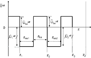
Figure 9: A model potential with two square wells of depth $|{\bar{U}}_{1}^{eff}|$ and $|{\bar{U}}_{2}^{eff}|$ within the range $z_{we1}$ and $z_{we2}$, and one barrier of height ${\bar{U}}_{ba}^{eff}$ and width $z_{ba}$. Because of the hard walls, the effective potential $V^{eff}=\infty$ for $z\leq 0$ and $z\geq z_{d}$.

The presence of repellers contribute the effective potentials of the stickers in Eq. (20). To make this point more transparent, let the effective potential of sticker-$i$ ($i=1$ or 2) in the absence of repellers be

$$[{\bar{U}}_{1}^{eff}]_{0}=-T\ln\frac{1+e^{(-U_{1}+\mu_{1})/T}+e^{\mu_{2}/T}}{1+e^{\mu_{1}/T}+e^{\mu_{2}/T}},$$ (21)

and

$$[{\bar{U}}_{2}^{eff}]_{0}=-T\ln\frac{1+e^{\mu_{1}/T}+e^{(-U_{2}+\mu_{2})/T}}{1+e^{\mu_{1}/T}+e^{\mu_{2}/T}}.$$ (22)

In the presence of repellers, the effective potentials become

$$[{\bar{U}}_{1}^{eff}]_{trans}=-T\ln\frac{1+e^{(-U_{1}+\mu_{1})/T}+e^{\mu_{2}/T}+e^{\mu_{3}/T}}{1+e^{\mu_{1}/T}+e^{\mu_{2}/T}+e^{\mu_{3}/T}},$$ (23)

$$[{\bar{U}}_{2}^{eff}]_{trans}=-T\ln\frac{1+e^{\mu_{1}/T}+e^{(-U_{2}+\mu_{2})/T}+e^{\mu_{3}/T}}{1+e^{\mu_{1}/T}+e^{\mu_{2}/T}+e^{\mu_{3}/T}},$$ (24)

and the effective potential of the repellers is

$${\bar{U}}_{ba}^{eff}=-T\ln\frac{1+e^{\mu_{1}/T}+e^{\mu_{2}/T}+e^{(-U_{3}+\mu_{3})/T}}{1+e^{\mu_{1}/T}+e^{\mu_{2}/T}+e^{\mu_{3}/T}}$$ (25)

Intuitively, adding repellers to the system reduces the affinity of the stickers, this can verified by straightforward algebra. Indeed, from Eqs. (21)(22)(23)(24), one finds

$$|[{\bar{U}}_{1}^{eff}]_{trans}| = |[{\bar{U}}_{1}^{eff}]_{0}|+T\ln\frac{1+e^{\mu_{3}/T}/\left[1+e^{(-U_{1}+\mu_{1})/T}+e^{\mu_{2}/T}\right]}{1+e^{\mu_{3}/T}/(1+e^{\mu_{1}/T}+e^{\mu_{2}/T})}$$ (26)

$$< |[{\bar{U}}_{1}^{eff}]_{0}|,$$

and

$$|[{\bar{U}}_{2}^{eff}]_{trans}| = |[{\bar{U}}_{2}^{eff}]_{0}|+T\ln\frac{1+e^{\mu_{3}/T}/\left[1+e^{\mu_{1}/T}+e^{(-U_{2}+\mu_{2})/T}\right]}{1+e^{\mu_{3}/T}/(1+e^{\mu_{1}/T}+e^{\mu_{2}/T})}$$ (27)

$$< |[{\bar{U}}_{1}^{eff}]_{0}|,$$

because $U_{1}<0$, and $U_{2}<0$.

The above discussion suggests that to see if the presence of repellers enhances or suppresses adhesion-induced lateral phase separation of different species of stickers, one needs to compare the critical potentials $|{\bar{U}}_{ic}^{eff}|$ in the presence of repellers with $|[{\bar{U}}_{ic}^{eff}]_{trans}|$, the potentials that are transformed from $|[{\bar{U}}_{ic}^{eff}]_{0}|$ by Eqs. (26)(27).

As demonstrated in the previous section, although quantitatively not accurate, mean field approximation gives us correct physical picture of the system under consideration. Since the precise magnitude of the critical potential depths is not the key issue of this section, we use mean field theory to study the effect of repellers. First we check if the effect of confinement in the presence of repellers is the same as that in the absence of repellers. The critical potential depths in the presence of repellers versus $z_{d}$ for $z_{1}=0.1$, $z_{3}=1.0$, $z_{ba}=0.4$, $z_{we1}=0.2$, $z_{we2}=0.2$, and $|{\bar{U}}_{ba}^{eff}|=0.1$ in the mean field approximation are shown in Fig.10a. Indeed, like the no-repeller case, the the critical potential depths $|{\bar{U}}_{1c}^{eff}|$ and $|{\bar{U}}_{2c}^{eff}|$ decrease as $z_{d}$ increases. Furthermore, the confinement effect is negligible for large values of $z_{d}$, this is also the same as no-repeller case.

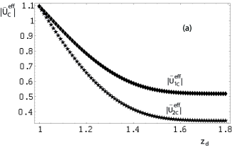
Figure 10: (a) The critical potential depths versus $z_{d}$ for $z_{1}=0.1$, $z_{3}=1.0$, $z_{ba}=0.4$, $z_{we1}=0.2$, $z_{we2}=0.2$, and $|{\bar{U}}_{ba}^{eff}|=0.1$. For small $z_{d}$, $|{\bar{U}}_{c}^{eff}|$ decreases as $z_{d}$ increases. (b) Upper curve: $|{\bar{U}}_{2c}^{eff}|-|[{\bar{U}}_{2c}^{eff}]_{trans}|=0$, lower curve: $|{\bar{U}}_{1c}^{eff}|-|[{\bar{U}}_{1c}^{eff}]_{trans}|=0$. On the left of the curves, repellers suppress lateral phase separation; on the right of the curves, repellers enhance lateral phase separation; between the curves, $|{\bar{U}}_{2c}^{eff}|-|[{\bar{U}}_{2c}^{eff}]_{trans}|<0$, and $|{\bar{U}}_{1c}^{eff}|-|[{\bar{U}}_{1c}^{eff}]_{trans}|>0$. The curves are plotted for $z_{1}=0.1$, $z_{3}=1$, $z_{d}=2$, $z_{we1}=0.2$, $z_{we2}=0.2$, and $z_{ba}=0.4$.

To see the effect of repellers on adhesion-induced phase separation, we compare the critical potentials of the stickers $|[{\bar{U}}_{ic}^{eff}]|$ with $|[{\bar{U}}_{ic}^{eff}]_{trans}|$. Figure 10b shows the curves on which $|{\bar{U}}_{ic}^{eff}|=|[{\bar{U}}_{ic}^{eff}]_{trans}|$ for $z_{1}=0.1$, $z_{d}=6$, $z_{we1}=z_{we2}=0.2$, and $z_{ba}=0.4$. Repellers suppress phase separation on the left of the curves, and enhance phase separation on the right of the curves. Between the curves $|{\bar{U}}_{2c}^{eff}|-|[{\bar{U}}_{2c}^{eff}]_{trans}|<0$, and $|{\bar{U}}_{1c}^{eff}|-|[{\bar{U}}_{1c}^{eff}]_{trans}|>0$. This indicates that stiff repellers enhance, while soft repellers suppress adhesion-induced lateral phase separation. This result can be understood by a simple analysis. When membrane-membrane collisions is not important, adding repellers should not significantly change the height of energy barrier between the wells of the stickers, thus the critical potentials of the stickers in the presence of repellers are related to those in the absence of repellers by $|{\bar{U}}_{ic}^{eff}|+{\bar{U}}_{ba}^{eff}\approx|[{\bar{U}}_{ic}^{eff}]_{0}|$. Repellers enhance phase separation as long as $|[{\bar{U}}_{ic}^{eff}]_{trans}|>|{\bar{U}}_{ic}^{eff}|\approx|[{\bar{U}}_{ic}^{eff}]_{0}|-{\bar{U}}_{ba}^{eff}$. From Eqs. (26)(27)(25), this condition leads to

$$T\ln\left[\frac{1+e^{\mu_{3}/T}/(1+e^{(-U_{1}+\mu_{1})/T}+e^{\mu_{2}/T})}{1+e^{(-U_{3}+\mu_{3})/T}/(1+e^{\mu_{1}/T}+e^{\mu_{2}/T})}\right]>0$$ (28)

for type-1 stickers. Since $U_{3}>0$, we find that for sufficiently large $U_{3}$ (i.e., stiff repellers) the above inequality is satisfied and phase separation is enhanced. Similarly, when $U_{3}$ is sufficiently large, $|{\bar{U}}_{2c}^{eff}|-|[{\bar{U}}_{2c}^{eff}]_{trans}|<0$.

4 Summary and conclusion

We have developed a mean field analysis that is convenient for studying the phase behavior of membrane adhesion induced lateral phase separation. Our study shows that vertical confinement tends to suppress adhesion-induced phase separation because long-sticker-rich state is suppressed due to the entropic loss. We also find that adding repellers reduce the effective binding energies of the stickers, and repellers play a non-trivial role in adhesion-induced phase separation: stiff repellers tend to enhance phase separation, soft repellers tend to suppress phase separation. These ideas are not difficult to check in experiments. For example, consider vesicle adhesion to supported membranes via two types of stickers. Our analysis predicts that it is possible to mix the phase-separated stickers by simply compressing the vesicle against the supporting substrate. The effect of repellers can be checked by incorporating non-adhesive flexible polymers and stiff rod-like molecules to the vesicle surface, and examine the adhesion zone. Flexible polymers should suppress lateral phase separation while stiff molecules should enhance lateral phase separation. We believe that these effects could be useful in the development of new sensitive soft materials with possible applications in future bio-technologies.

References

- [1] R. Lipowsky and E. Sackmann., Structure and Dynamics of Membranes: Generic and Specific Interactions, Vol. 1B of Handbook of Biological Physics (Elsevier, Amsterdam 1995).
- [2] B. Alberts ., , 3rd edition (Garland, New York, 1994).
- [3] S. Komura and D. Andelman, Eur. Phys. J. E 3, 259 (2000).
- [4] R. Bruinsma, A. Behrisch, and E. Sackmann, Phys. Rev. E 61, 4253 (2000).
- [5] A. Albersd fer, T. Feder, and E. Sackmann, Biophys. J. 73, 245 (1997).
- [6] T. R. Weikl, R. R. Netz, and R. Lipowsky, Phys. Rev. E 62, R45 (2000).
- [7] J. Nardi, T. Feder, and E. Sackmann, Europhys. Lett. 37, 371 (1997).
- [8] T. R. Weikl and R. Lipowsky, Phys. Rev. E 64, 011903 (2001).
- [9] H. Strey, M. Peterson, and E. Sackmann, Biophys. J. 69, 478 (1995).
- [10] D. Zuckerman and R. Bruinsma, Phys. Rev. Lett. 74, 3900 (1995).
- [11] C. R. F. Monks et al., Nature (London) 395, 82 (1998); G. Grakoui et al., Science, 285, 221 (1999); D. M. Davis et al., Proc. Natl. Acad. Sci. U.S.A. 96, 15062 (1999).
- [12] S. Y. Qi, J. T. Groves, and A. K. Chakraborty, Proc. Natl. Acad. Sci. U.S.A. 98, 6548 (2001).
- [13] N. J. Burroughs and C. Wlfing, Biophys. J. 83, 1784 (2002).
- [14] T. R. Weikl and R. Lipowsky, Biophys. J. 87, 3665 (2004).
- [15] H.-Y. Chen, Phys. Rev. E 67, 031919 (2003).
- [16] Jia-Yuan Wu and H.-Y. Chen, Phys. Rev. E 73, 011914 (2006).
- [17] M. Asfaw, B. Rozycki, R. Lipowsky and T. R. Weikl, Europhys. Lett. 76, 703 (2006).
- [18] R. Lipowsky, J. Phys. II France 4, 1755 (1994).
- [19] A. Ammann, R. Lipowsky, J. Phys. II France 6, 255 (1996).
- [20] K. Binder and D. W. Heermann, Monte Carlo Simulation in Statistical Physics (Springer, Berlin) 1992.
- [21] Mesfin Asfaw, Ph.D. thesis, Max Planck institute for Colloids and Interfaces, Potsdam, Germany (2005), (unpublished).