Probing Spectroscopic Variability of Galaxies & Narrow-Line Active Galactic Nuclei in the Sloan Digital Sky Survey

Abstract

Under the unified model for active galactic nuclei (AGNs), narrow-line (Type 2) AGNs are, in fact, broad-line (Type 1) AGNs but each with a heavily obscured accretion disk. We would therefore expect the optical continuum emission from Type 2 AGN to be composed mainly of stellar light and non-variable on the time-scales of months to years. In this work we probe the spectroscopic variability of galaxies and narrow-line AGNs using the multi-epoch data in the Sloan Digital Sky Survey (SDSS) Data Release 6. The sample contains 18,435 sources for which there exist pairs of spectroscopic observations (with a maximum separation in time of $\sim{700}$ days) covering a wavelength range of $3900-8900$ Å. To obtain a reliable repeatability measurement between each spectral pair, we consider a number of techniques for spectrophotometric calibration resulting in an improved spectrophotometric calibration of a factor of two. From these data we find no obvious continuum and emission-line variability in the narrow-line AGNs on average – the spectroscopic variability of the continuum is $0.07\pm 0.26$ mag  in the $g$ band and, for the emission-line ratios $\log_{10}$($[$N II$]$/H$\alpha$) and $\log_{10}$($[$O III$]$/H$\beta$), the variability is $0.02\pm 0.03$ dex and $0.06\pm 0.08$ dex, respectively. From the continuum variability measurement we set an upper limit on the ratio between the flux of varying spectral component, presumably related to AGN activities, and that of host galaxy to be $\sim{30}$%. We provide the corresponding upper limits for other spectral classes, including those from the BPT diagram, eClass galaxy classification, stars and quasars.

1. Introduction

Active galactic nuclei (AGNs) are found to vary in the time-domain at many frequencies. The underlying physical mechanism driving the variability seen in AGN spectra is unknown (e.g., Peterson, 2001; Bono et al., 2003). Several scenarios have been proposed including accretion disk instability (Kawaguchi et al., 1998), supernova explosion (Aretxaga et al., 1997), microlensing by stars in the intervening galaxy (Hawkins, 1993), and varying ionizing source or/and varying optical depth of the material in the vicinity of light-generating regions (e.g., Tohline & Osterbrock, 1976; Goodrich, 1989). At present, models involving non-thermal emission from the jets or events occurring on the AGN accretion disk are most favored (see, e.g., Stalin et al., 2004, for a summary of variability models in AGNs by radio loudness).

Most variability studies, however, have been focused on Type 1 (broad-line) AGNs. While the emission lines of Type 2 (narrow-line) AGNs were found to vary in the X-rays on time-scales from hours to years (Guainazzi et al., 1998; Mueller et al., 2003; Mateos et al., 2007), their optical continua and emission lines are generally considered to be non-variable. For the emissions from the narrow-line regions, the spatially low-density region (electron density $n_{e}\sim{1,000}$ cm^-3) results in a long ($\sim{100}$ years) recombination time (Peterson et al., 1995), exceeding the duration of a typical observation. For the optical continuum, it is commonly considered to be composed mainly of the stellar light, in accord with the expectation from the unification model (Antonucci, 1993; Urry & Padovani, 1995) in which Type 2 objects are obscured by a dusty torus along the line-of-sight. Dominated by the stellar light, the optical continuum in Type 2 AGNs should therefore be temporally non-variable. There is, however, no strong observational evidence in the time-domain to either support or dispute these ideas.

From a 4-year monitoring of the broad-band optical variability of 35 Type 1 and 2 Seyfert galaxies, Winkler et al. (1992) demonstrated that most galaxies in their sample were variable. Another promising work to probe Type 2 AGN variability in the optical is the intra-night variability of Seyfert 2 galaxies observed by Jang (2001), where two out of the three objects varied by $\sim{0.25}$ mag. Further, Trippe et al. (2008) found a Type 1.9 Seyfert galaxy (Osterbrock, 1989) to change into a Type 2 Seyfert over a few years, and proposed the underlying cause to be a varying ionizing continuum.

The UV-optical variability of broad-line AGNs is better established with an amplitude of $\sim{10\%}$ (e.g., see discussions in Vanden Berk et al., 2004). Wavelength dependence of QSO variability has been studied by Wilhite et al. (2005), and the C IV-emission dependence by Wilhite et al. (2006) in the Sloan Digital Sky Survey (SDSS, York et al., 2000). In these studies the authors have developed a method to remove wavelength-dependent systematics which may exist in the spectra, from a spectroscopic plate at one epoch of observation to the same plate at another epoch. Correcting for this on a plate-to-plate basis they were able to select variable QSOs and to demonstrate a power-law-like QSO difference spectrum; which in turn can be explained by the change in the accretion rate in thermal accretion disk (Pereyra et al., 2006). QSO photometric variability in the SDSS has been studied by Vanden Berk et al. (2004) for its dependency on physical parameters such as redshift, luminosity and radio properties; by de Vries et al. (2003) in which the authors used both the SDSS and the historical observations (up to $\sim{50}$ years) and found the time-scale of the variability to be $\sim{2}$ years; and by Ivezić et al. (2004) and Sesar et al. (2006) in which the authors used the SDSS repeated imagings in combination with the Palomar Observatory Sky Survey (POSS) data to probe long term QSO variability (up to $\sim{50}$ years), and constrained its time scale to be $\sim{1}$ year in the restframe.

Normal “inactive” galaxies (for our purpose defined to be galaxies that are not Type 1 or Type 2 AGNs, nor low-ionization nuclear emission regions – (LINERS, Heckman, 1980)) are not observed to be variable; and are generally not expected to be. For the continua of galaxies, the time scale of observation is negligible compared with that of stellar evolution (for solar-mass main sequence stars, lifetime $\approx{10^{10}}$ years). For emission-line regions, that arise from low-density environments and H II regions, similar arguments can be made to those for narrow-line regions, with the understanding that the electron density is likely to be lower ($n_{e}\sim{1-1,000}$ cm^-3, Spitzer, 1978).

The goal of this work is, therefore, to probe spectral variability of galaxies and narrow-line AGNs using the SDSS multi-epoch observations. The SDSS data have the advantage of large sample size with the same spectrophotometric reduction, which is critical to our work because we expect any variability present in galaxies to be small (compared with the amplitude of the QSO UV-optical variability, for example). Several techniques are used to refine the spectroscopic calibration, including those by Wilhite et al. (2005). The resultant galaxy variability measurement is compared with that of stars and QSOs, independently analyzed in this work.

In §2 we discuss the samples used. In §3 we present the variability measure. In §4 we describe the refinement of the spectroscopic calibration. In §5 we present the galaxy continuum variability, and the emission line variability of the variable candidates based on the continuum. In §6 we present results on variability analyses on stars and QSOs as sanity checks. In §7 we summarize the results and discuss future work.

2. Samples

As part of the SDSS (York et al., 2000) spectra are observed with fibers of 3″  diameter (corresponding to 0.18 mm at the focal plane for the 2.5 m, f/5 telescope, Gunn et al., 2006). The spectral resolution $R$ is $\sim{1800}$ in the observed frame $3800-9200$ Å. All sources are selected (or “targeted”) from an initial imaging survey using the SDSS camera as described in Gunn et al. (1998) with the filter response curves as described in Fukugita et al. (1996), and using the imaging processing pipeline of Lupton et al. (2001). The astrometric calibration is described in Pier et al. (2003). The photometric system and calibration are described in Fukugita et al. (1996), Hogg et al. (2001), Smith et al. (2002) and Ivezić et al. (2004), Tucker et al. (2006). The targeting strategy for the multi-object spectrograph is described in Blanton et al. (2003).

We select our samples from the Data Release 6 (DR6, Adelman-McCarthy et al., 2008) of the SDSS. The galaxy sample is constructed from the SDSS Main Galaxy sample (Strauss et al., 2002), by selecting spectra which are both spectroscopically classified as galaxies, and rejecting spectra in which the redshift measurements failed or have not been made. The spectral classification (star, galaxy, QSO) is highly confident, with 98% of all the DR6 spectra having consistent classification between the spectro1d pipeline (SubbaRao et al., 2002) and the specBS pipeline (Schlegel et al. in prep.). From this sample, pairs of spectral observations are identified by matching sources in both RA and DEC to within 1″, and in redshift to within 0.01. Spectra at both epochs are required to have the same plate number but different date of observations, given in Modified Julian Date (MJD) by the SDSS. The selection results in 23,330 pairs. The subsequent sample selections (mainly for the purpose of increasing the signal-to-noise, S/N, of the spectra) will be described in §4 and §5. Table LABEL:tab:plate lists the relevant spectroscopic plates and the corresponding number of galaxy spectra. The sample covers $\sim{3-700}$ days in the observed frame.

The spectroscopically classified galaxies selected above do not contain any strong (equivalent width, EW $>$10 Å, and $>3\sigma$  detection in the height of the line) broad line (full width at half maximum, FWHM $>$1000 km s^-1) (SubbaRao et al., 2002). The cutoff is below the traditional line-width selection for broad lines (Type 1) galaxies, where the width of permitted line(s) $>2000$ km s^-1 (e.g., Komossa, 2008). The sample therefore comprises galaxies of different eClass types (Connolly et al., 1995), and narrow-line AGNs. A potential contamination to our galaxy sample would be the narrow-line Seyfert 1 galaxies (Osterbrock & Pogge, 1985, and references therein), expected to offer a direct view of the active nuclei (Antonucci, 1993; Urry & Padovani, 1995) and can be variable in the optical (Giannuzzo & Stirpe, 1996; Peterson et al., 2000). Each of these spectra shows a broad component in Balmer emission line with FWHM $<2000$ km s^-1, and relatively weak $[$O III$]\lambda$5008. The reasons behind this potential contamination are twofold – firstly, the spectro1d pipeline fits to each line a single Gaussian, that may underestimate the line width of the broad component in the case of a composite line which is made up of both the broad and narrow components, in particular when the broad one is relatively weak. Secondly, the FWHM of the broad component of both H$\alpha$ and H$\beta$  of a narrow-line Seyfert 1 can extend down to $\sim 500$ km s^-1 (Fig. 4 of Zhou et al., 2006), falling within the galaxy spectral classification in the SDSS. However, we expect the number contribution of these objects to the whole DR6 galaxy+QSO sample to be small, $\sim 0.5$%, with reference to Zhou et al. (2006) who used an upper limit of $2200$ km s^-1 in the broad component of H$\alpha$ or H$\beta$  emissions to search for narrow-line Seyfert 1 in the SDSS. Similarly, the Seyfert 1.8 and 1.9 (Osterbrock, 1989), both of which show strong narrow components (relative to the broad ones, if available) in H$\alpha$  and H$\beta$, can be variable in the optical (Goodrich, 1989), and may be present in our galaxy sample as well. We note that the current analysis does not provide further separation of those from our emission-line galaxies, that calls for fitting of double Gaussian to each Balmer line, for example. The number contribution of these types to the full galaxy sample is expected to be small, $\sim 0.02$% (Wang & Wei, 2008). In this work, the fraction of the classified Seyfert 2 + starforming + composite galaxies to the full sample of our galaxy spectral pairs is $\sim 14$%; and that of all the eClass types, $\sim 22$% (calculated from Table 4).

When constructing the stellar and QSO samples, the spectral pairs are selected similarly to the case of galaxies, except that they are spectroscopically classified as star and QSO, respectively. The targeting selection for spectroscopic observation of QSOs in the SDSS is described in Richards et al. (2002). Each QSO spectrum classified (SubbaRao et al., 2002) has at least one strong line (see above for the galaxy classification) with FWHM $>$1000 km s^-1, or/and a Lyman alpha forest. Unlike the selection of the galaxies and the QSOs, no criterion is imposed on the quality of the redshift when selecting the stars. The upper bound of their distances is $cz=450$ km s^-1, or $z=0.0015$ (SubbaRao et al., 2002). The samples contain 9,100 stellar pairs and 3,205 QSO pairs (0.08 $<z<$ 3.51), respectively.

The spectra are de-reddened against Galactic extinction using the library written by Simon Krughoff, which adopts the SFD dust maps (Schlegel et al., 1998) and the extinction curve by O’Donnell (1994). Following the SDSS convention the spectra are expressed in vacuum wavelengths. Flux densities $f_{\lambda}$ are expressed in $10^{-17}$ ergs s^-1 cm^-2 Å^-1.

3. Variability Amplitude: $F_{\mathrm{var}}$

We adopt the dimensionless variability measure, $F_{\mathrm{var}}$, for $N$-epoch repeated observations (e.g., Rodriguez-Pascual et al., 1997; Peterson, 2001). It is a fractional root-mean-squared variability amplitude defined as

$$F_{\mathrm{var}}=\frac{\sqrt{\sigma^{2}-\delta^{2}}}{\langle f\rangle}\ ,$$ (1)

where $\sigma^{2}$ is the variance of the flux, $\delta^{2}$ is the mean square uncertainty of the flux, and $\langle f\rangle$ is the mean flux

$$\sigma^{2} = \frac{1}{N}\sum_{i=1}^{N}{(f_{i}-\langle f\rangle)}^{2}\ ,$$ (2)

$$\delta^{2} = \frac{1}{N}\sum_{i=1}^{N}\delta_{i}^{2}\ ,$$ (3)

$$\langle f\rangle = \frac{1}{N}\sum_{i=1}^{N}f_{i}\ .$$ (4)

The numerator, proposed by Bonoli et al. (1979), was termed the square-root of the “excess variance” (Vaughan et al., 2003), in the sense that the flux uncertainty is subtracted in quadrature from the variability. In the calculation of the continuum $F_{\mathrm{var}}$ the wavelength intervals encompassing emission-line center wavelengths $\pm$ 280 km s^-1  are excluded (using the vacuum wavelength values in the line list adopted by the SDSS, and excluding the lines Ca K and H, H$\delta$, the G band around 4306 Å, Mg$\lambda$5177, Na$\lambda$5896, and the Ca II triplet that usually appear as absorptions). The mean square uncertainty for the spectrum at each epoch ($\delta_{i}^{2}$ for a given $i$) is calculated by quadrature summation of the pipeline flux uncertainty per pixel, over all valid pixels. It is therefore a variance in flux based on photon statistics. A valid pixel is defined to be a pixel that is not flagged as bad. The flags are listed in §4.2. $F_{\mathrm{var}}$ is calculated in the observed frame with wavelengths $3900-8900$ Å for each object and for all spectral types.

When calculating $F_{\mathrm{var}}$  for narrow-line AGNs, since any possible host-galaxy contribution is not explicitly subtracted from an observed spectrum, the full observed spectrum is used in calculating the denominator $\langle f\rangle$. As the numerator term “excess variance” does not contain the non-variable host-galaxy contribution, the resultant $F_{\mathrm{var}}$  is therefore a lower limit on the AGN variability.

If the excess variance $\sigma^{2}-\delta^{2}<0$, we assume the variability is zero for the object, but continue to include it in the analysis. In this work, $N=2$. We note that any non-zero $F_{\mathrm{var}}$ is referred to as a “variability” measurement, regardless of the origin being physically interesting or otherwise.

4. Refining Spectroscopic Calibration

The principal steps in the spectrophotometric calibration of each spectrum in the SDSS are: a wavelength-dependent calibration using the observed standard stars on the same plate; and the tying of the absolute flux scale to the observed PSF magnitudes of stars, on the same plate (Adelman-McCarthy et al., 2008). The resultant average uncertainty in the spectrophotometry for DR6 is $7\%$ at observed frame wavelength $3800$ Å  (Adelman-McCarthy et al., 2008). As any variability in the sources from our sample is expected to be of low amplitude, the calibration of the pipeline spectra must be improved using the approaches described below.

4.1. Wavelength-dependent correction

We adopt the method developed by Wilhite et al. (2005) to remove systematics which may be present in each pair of galaxy spectra taken on separate MJDs. Flux-density corrections as a function of the observed-frame wavelength in the range of $3900-8900$ Å  are calculated by a linear fit (tied to the origin) between the flux density ($f_{\lambda}$) of all the objects at epoch 2 (the later epoch) and those at epoch 1. This calculation results in a calibration spectrum for one plate. We adopt a slightly different methodology from Wilhite et al. (2005) in which stellar spectra in each plate were used. Our calibration spectrum per plate is calculated using all galaxies present in that plate, as we want to maximize the number of objects in generating the calibration spectrum, and avoid potential systematic effects when applying point source calibration to extended sources. The underlying assumption is that the majority of the galaxies observed in a given plate are non-variable in time across the two epochs. Even if the galaxies were in fact variable, the method is still applicable because the variable amplitude of several hundred galaxies is not expected to be in phase. An example calibration spectrum is plotted in Fig. 1. Typically the calibration spectra are smooth. To focus on low-order corrections to the galaxy spectra, and to remove noise in the calibration spectrum, we follow Wilhite et al. (2005) and set the final calibration spectrum per plate as its 5th-order polynomial least-squares fit. By visual inspection this functional form works well in removing higher-order spurious spectral features.

When constructing the calibration spectrum we drop any plate in which there are less than 10 pairs of galaxy spectra. We then refine each and every spectrum present in a given plate by using the calibration spectrum, if available.

4.2. Wavelength-independent correction

After removing wavelength-dependent systematics, each spectral pair can, in principle, be subjected to a wavelength-independent normalization in their flux densities. In order to obtain an accurate variability measurement of each spectral pair, the total continuum fluxes of the two spectra at a chosen common wavelength region are set equal. Specifically, for each pair the galaxy spectrum at the epoch of lower S/N is shifted in a wavelength-independent fashion according to

$${f_{\lambda}}^{\mathrm{(low\,\rm S/N)}}{\mathrm{(corrected)}}=C_{\mathrm{band}}\,{f_{\lambda}}^{\mathrm{(low\,\rm S/N)}}{\mathrm{(original)}}\ ,$$ (5)

in which $C_{\mathrm{band}}$ is a constant for each spectral pair, calculated as

$$C_{\mathrm{band}}={F_{\lambda\in{\mathrm{band}}}}^{\mathrm{(high\,\rm S/N)}}/{F_{\lambda\in{\mathrm{band}}}}^{\mathrm{(low\,\rm S/N)}}\ ,$$ (6)

where $F_{\lambda\in\mathrm{band}}$ is the total flux in the restframe wavelength range (which is referred to as “rest-band” for convenience). In this work the rest-band is chosen to be 6450 Å $\pm~{}520$ km s^-1, as such no prominent emission lines are present in the galaxy spectra. Only the galaxy spectra in the first epoch are re-calibrated because it is typically the existence of low S/N data that results in a second observation. The combined procedure of systematics removal and restframe band scaling is referred to “SYS+BAND” in the following discussion.

Given an initial sample (§2, 23,330 objects), we impose S/N cuts using the rest-band measures (or the $[$O III$]\lambda$5008 (vacuum) line, described later when we discuss absolute flux calibration). In this case we reject any spectral pair if there are one or more pixels flagged in either or both spectra in the wavelength region of interest, and we require the flux to be larger than zero at both epochs. The flags under consideration are NOPLUG, BADTRACE, BADFLAT, BADARC, MANYBADCOL, MANYREJECT, LARGESHIFT, FULLREJECT, SCATTERLIGHT, CROSSTALK, NOSKY, BRIGHTSKY, NODATA, COMBINEREJ, BADFLUXFACTOR, BADSKYCHI and REDMONSTER. All of the spectral flux or S/N calculations in this paper are carried out with pixel-masking using these flags. After this S/N criteria, the number of objects in the galaxy sample is reduced to 18,435 (Table LABEL:tab:plate).

In Fig. 2 and 3 we show the restframe galaxy spectra in two epochs from the SDSS pipeline and after the calibration refinement, respectively. Firstly, we note that the pipeline performs well, that the fractional difference between both epoch is about 10% at the shortest wavelength, which is sufficient for many spectral analyses involving emission or absorption lines. However, continuum residual in Fig. 2 is present, which induces a variability ($F_{\mathrm{var}}=0.058$). After the calibration refinement we are able to obtain a zero continuum variability.

For comparing with the rest-band scaling previously discussed, we also adopt the absolute flux calibration described in Peterson et al. (1998). In this procedure, the spectrum in the low S/N epoch in the duo is scaled wavelength-independently so that its total flux in $[$O III$]\lambda$5008 (vacuum) is the same as that of the spectrum in the high S/N epoch. The physical justification is that the $[$O III$]\lambda$5008 line generally appears as a narrow line arising from a low-density region, which is believed to be non-variable in time (Peterson et al., 1995). We note that the average $[$O III$]$ EW of galaxy spectra in the full DR6 catalog is a few Å, so for some objects mainly the continuum flux is measured and is expected to be non-variable as well. The combined procedure of systematics removal and absolute $[$O III$]$ calibration is called “SYS+OIII” in the following. The region of influence is set to be 5008 Å $\pm~{}280$ km s^-1.

When judging which method performs better in analyzing spectral variability, we consider the better method to be the one which minimizes the mean, one standard deviation of the mean ($\sigma_{m}$) and the one standard deviation sample scatter ($\sigma$) of the variability at a fixed spectral S/N. These statistics for the galaxy sample by using the SYS+BAND, SYS+OIII and other refinement methods are listed in Table 2. At S/N $\geq 10$ the SYS+BAND method produces smaller mean and scatter in $F_{\mathrm{var}}$. The difference is not related to the difference in the width of the rest-band being used (520 km s^-1 vs 280 km s^-1), as the SYS+BAND method is also re-performed using 6450 Å $\pm~{}280$ km s^-1, the same width as in the SYS+OIII method. These statistics remain lower in value than those in the SYS+OIII even for this reduced interval. The result suggests that the $[$O III$]\lambda$5008 line in some spectra may be impacted by the effect of seeing so that the total observed line flux is different for the two epochs. The other possible reasons for this discrepancy are: the total line flux is sampled at only a few wavelength bins in the medium resolution SDSS spectra, or the line may exhibit intrinsic variability.

To further test the method SYS+BAND, we divide the galaxy sample into RED and BLUE galaxies by using the eClass classification (described in §5.2.1). The RED spectra are defined as objects with classification parameter $\phi_{KL}\geq 0^{o}$, and the BLUE galaxies, $\phi_{KL}<0^{o}$. For each plate, the calibration spectrum is calculated using only the RED or BLUE galaxies, which in turn is used to re-calibrate galaxies of all spectral types on the same plate. The purpose behind this is to determine whether the refinement method SYS+BAND would be biased by the presence of potentially different galaxy spectral types in the plate. We find that using a specific spectral type does not cause the variability statistics to change (Table 2). We therefore adopt SYS+BAND as the calibration method, and use all available galaxy spectral types when calculating the calibration spectrum throughout this work. The “before and after” of this approach is shown in Fig. 4, where we see that the scatter in $F_{\mathrm{var}}$  vs. S/N of our galaxy sample is reduced after the refinement. Comparing the average variability of our galaxy sample using the SYS+BAND approach with that from the original SDSS spectral reductions (Table 2) we find that the spectrophotometry is improved by a factor of two.

4.3. Plate-to-Plate Difference

There are plate-to-plate differences seen in the above definitions of variable and non-variable sources, that is, the best-fit coefficients in Eqn. 7 are in general plate dependent. In Fig. 5 we show $\langle F_{\mathrm{var}}\rangle$ of the galaxy spectra vs. average spectral S/N, per plate. The average $F_{\mathrm{var}}$ per plate is larger at lower overall spectral S/N, suggesting in those plates the variability measurement is likely affected by the presence of noise in the spectra. By dropping individual spectral pairs with spectral S/N $<10$ at the second epoch, the average and the sample scatter in $F_{\mathrm{var}}$ are reduced to $0.010$ and $0.003$, respectively.

5. Galaxy Variability

5.1. Defining Variables

Following Wilhite et al. (2005) we define the variable candidates by objects having

$$F_{\mathrm{var}}(\rm S/N)>b_{0}\exp\left({\frac{\rm S/N}{b_{1}}}\right)+\,b_{2}\ .$$ (7)

The S/N of each spectrum is calculated in the second epoch and by using all of the valid pixels as defined in §4.2. The constants $b_{0},b_{1},b_{2}$ are determined by least-squares fitting the above exponential form to the binned data ($\langle\mathrm{S/N}\rangle$, $\langle F_{\mathrm{var}}\rangle+n\,\sigma(F_{\mathrm{var}})$), where $\sigma(F_{\mathrm{var}})$ is one standard deviation of $F_{\mathrm{var}}$ in each bin, and for $n=0,1,2,3,4$. Typically 10 bins in S/N are used.

The variable candidates (for galaxies, stars and QSOs) in this work are defined as objects with $>3\sigma$  detection. We do not sub-divide the distribution for detections greater than $4\sigma$, though in the future we plan to explore in more detail the tail of the variable distributions. For comparison we have also defined variables as objects located in a fixed upper percentile of $F_{\mathrm{var}}$ in the plot $F_{\mathrm{var}}$ vs. S/N. The $>3\sigma$ cut is equivalent to a $2-6$% upper percentile for a given S/N (Table 3).

5.2. Continuum

To explore any dependence of spectral variability or repeatability on the spectral type of galaxies, we divide the galaxy sample using two different spectral classification schemes: eClass (Connolly et al., 1995) and the “BPT” diagrams or the Osterbrock diagrams (Baldwin et al., 1981; Veilleux & Osterbrock, 1987). These two schemes are motivated by different spectral features. The eClass is a spectral type describing the steepness of the continuum slope and other higher-order spectral features by using a linear combination of several eigenspectra for each galaxy spectrum. The eClass parameters, $\phi_{KL}$ and $\theta_{KL}$, are related to the coefficients in the eigenspectra expansion (called eigencoefficients), which are calculated by the Spectro1d pipeline in the SDSS. Specifically, the angle $\phi_{KL}$ correlates with the H$\alpha$ emission EW (Madgwick et al., 2003) which is an indicator of star formation rate. The angle $\theta_{KL}$ discriminates galaxy spectra exhibiting post-starburst activities (Connolly et al., 1995; Yip et al., 2004).

On the other hand, the BPT diagrams separate the narrow-line AGNs from galaxies such as the star-forming galaxies by emission line ratios which indicate the physical conditions of gas inside the galaxies such as the electron density and the mean level of ionization (Osterbrock, 1989). The objects in these two spectral classification schemes are not mutually exclusive. We hereafter present results on variability within both kinds of classification.

5.2.1 eClass

The spectral variability as a function of S/N per mean eClass galaxy type (Connolly et al., 1995) is shown in Table 4, and Table 5 for only the variable candidates. The mean eClass spectra are galaxy spectra where each is averaged over a non-trivial size of subspace of the two eClass parameters $\phi_{KL}$ and $\theta_{KL}$ (Yip et al., 2004). Limited by the number of spectral pairs, $\leq~{}3$  in types E or F, only the types A, B, C and D are considered in the variable candidates (Table 5). The continuum of the mean galaxy spectrum is reddest in the type A and bluest in the type D.

Firstly, we note that the average variability amplitude are consistent among different eClass types to within 1–2$\sigma$ sample scatter. If we assume a priori that some populations of galaxies do not vary in time, then a spectral repeatability can be assigned to the population with the smallest mean and scatter in $F_{\mathrm{var}}$, that is, the mean eClass type B. The spectral features of this class are similar to the elliptical galaxies in the atlas of nearby galaxies by Kennicutt (1992). The repeatability, taken to be the average $F_{\mathrm{var}}$, is 0.010 or 1.0%  in the observed-frame wavelength range $3900-8900$ Å.

5.2.2 Emission-line galaxies: narrow-line AGN vs. star-forming

Emission-line galaxies are considered by using the BPT diagram, using the starburst theoretical modeling line by Kewley et al. (2006). We consider the types: Seyfert 2, star-forming, composite and LINERs (Heckman, 1980). We do not find any LINER in our galaxy spectral pairs, using the classification criteria by Kewley et al. (2006, their Eqn. 15) which involved $[$O I$]$$\lambda{6302}$. We hereby consider the diagram log₁₀$([$O III$]$/H$\beta$) vs. log₁₀($[$N II$]$/H$\alpha$) (Fig. 5 of Baldwin et al., 1981).

In the first step of this analysis the EWs are taken from the SDSS reduction. Galaxies with any one of the four lines (H$\beta$  at $4863$ Å, [O III]$\lambda$5008, H$\alpha$  at $6565$ Å, [N II]$\lambda$6585) having restframe EW smaller than $1$ Å are rejected (in the SDSS convention EW $>0$ for emission lines); and at least a 2$\sigma$  detection is required in each of the four lines. Restframe stellar absorption of the related hydrogen emission lines in the BPT diagram is corrected for by a constant increment of 1.3 Å  (Hopkins et al., 2003; Miller et al., 2003). Any possible aperture effect on the emission lines is neglected in this paper, because the primary interest of this work is the comparison of line strength between two epochs, which is done using the same aperture for each object in each epoch and will only be subject to the difference in seeing. To correct on an object-by-object basis would require an assumption of an average line strength as a function of radius for each galaxy. Although the true line-flux correction of individual objects should depend on the distribution of the gas and its projected angle on the sky relative to the observational aperture, under the typical sky conditions in the SDSS observation (the median PSF width = 1.4″  in the $r$ band, Fig. 4 of Abazajian et al., 2003) and given the diameter of the fiber, the seeing-induced aperture correction factor to [O III] is close to unity, based on a nearby ($z=0.009$) Seyfert 1 with a well-resolved ($\sim{10}$″) narrow-line region (Fig. 3 of Wanders et al., 1992). This means that seeing-induced differences in the [O III] flux between any two epochs should be small. Further, the SDSS 3″  diameter fiber spectroscopy does not cause substantial aperture bias in classifying galaxy spectra based on emission lines (Miller et al., 2003).

In Table 4 we compare the variability amplitude between the star-forming galaxies and the narrow-line AGNs in the full galaxy sample, and Table 5 for the variable candidates. It is a little surprising that the average variability amplitude at S/N $\geq 10$  is $1.2\%$ for the star-forming galaxies, slightly higher than that of the narrow-line AGNs, $0.9\%$. The difference is bigger than 1$\sigma_{m}$ (i.e., the measurement of the $F_{\mathrm{var}}$  difference is reliable), but smaller than the $1\sigma$ sample scatter, indicating the $F_{\mathrm{var}}$ of both types are consistent with each other.

In Table 6 we show the average absolute AB magnitudes in $g,r$ and $i$ bands of variable candidates in the dim phase, and the sample-averaged magnitude difference between the dim and bright phases, per spectral type. The magnitudes are calculated for each spectrum, by convolving each restframe-shifted spectrum with the SDSS filter response curves for extended sources at an airmass of 1.3 (Fukugita et al., 1996), and in the AB filter system (Oke & Gunn, 1983). The average difference in the $g$-band magnitudes ranges from $0.07-0.10$ mag depending on the spectral type, but they are consistent among different spectral types to within $1\sigma$  sample scatter of the magnitude difference, $\sigma(\Delta{M})$, a measure of the sum of the sample scatters in both the distributions of $M(\textrm{dim})$ and $M(\textrm{bright})$. For the narrow-line AGNs, no obvious continuum variability is found (e.g., $0.07\pm 0.26$ mag in the $g$ band).

We note that the distribution of $F_{\mathrm{var}}$  in the full sample is non-Gaussian. Using the $>3\sigma$ cut for the variable candidates, for a Gaussian distribution one would expect the ratio between the number of variable candidates and that of the whole sample to be

$$\frac{1-\mathit{erf}(3/\sqrt{2})}{1-\mathit{erf}(-\infty)}\ ,$$ (8)

or $0.13$ %,where $\mathit{erf}(z)$ is the error function, and $1-\mathit{erf}(z)$ is the complementary error function of the form $(2/\sqrt{\pi})\int_{z}^{\infty}\,e^{-t^{2}}dt$. From Table 3, we see that typically at various S/N the $F_{\mathrm{var}}$ of the variable candidates span a longer tail ($1.53-3.44$ %).

5.2.3 Structure Function of the Continuum

The characteristic time scale of variability is usually studied by constructing the structure function (SF, e.g., Simonetti et al. (1985), Hughes et al. (1992); and references therein), the variability amplitude $F_{\mathrm{var}}$ as a function of time lag. Although no obvious continuum variability is found in our sample of galaxies on average, the SF is nonetheless constructed for the galaxy sample. Through the SF analysis, an absence of a time scale would be a cross-check of the lack of variability, and the comparison between the SF  of stars and of QSOs (§6) with that of the galaxies can be carried out.

The restframe SF, $F_{\mathrm{var}}$  vs. $\Delta\tau_{\mathrm{r}est}$, of all galaxies in the galaxy sample is illustrated in Fig. 6, where $\Delta\tau_{\mathrm{r}est}=\Delta\tau/(1+z)$, and $z$ being the redshift of a given galaxy. The time lag $\Delta\tau$ is the difference between the two MJDs of observation, MJD(epoch 2)$-$MJD(epoch 1). No obvious time-scale is seen in the above restframe SFs of galaxies for the $0-500$  days (restframe) sampled. A similar conclusion is obtained when the fractional change in flux ($|$$\Delta{f}/{f}$$|$) is used instead of $F_{\mathrm{var}}$ (Fig. 7), where $\Delta{f}$ is the difference in the flux between two epochs, and $f$ is the average flux over the two epochs.

An exponential function of the form

$$F_{\mathrm{var}}=a\,(1-b\,e^{-\Delta\tau_{\mathrm{r}est}/\tau_{s}})$$ (9)

is fitted to each structure function, where $\tau_{s}$  is the characteristic variability time scale. Typically, a structure function where $b=1$ is considered (e.g., Bonoli et al., 1979; Trevese et al., 1994). Firstly we relax $b$ to accommodate the non-zero variability at zero time lag, obvious in Fig. 6. This can be attributed to the repeatability of the continuum variability measurement (§5.2.1) in eClass Type B, where the mean $F_{\mathrm{var}}$ is 0.010 or 1.0%. The best-fit $\tau_{s}$ for the galaxies is $\sim{10}$ years. Uncertainty of this time scale is large ($\sim{2}$ years, with a reduced $\chi^{2}$ of $20$) because the duration of the observation is much shorter than the best-fit $\tau_{s}$.

We then consider a typical $b=1$ structure functional form at Eqn. 9. By assuming $F_{\mathrm{var}}$  at the zero time lag ($F_{\mathrm{var}}$$(0)$) (the noise) is uncorrelated with the intrinsic $F_{\mathrm{var}}$(the signal), one can obtain the intrinsic $F_{\mathrm{var}}$  by subtracting $F_{\mathrm{var}}$$(0)$ from the total $F_{\mathrm{var}}$ in a quadrature fashion. The resultant structure function is shown in Fig. 8, and the best-fit variability time scales in Table 8, where $F_{\mathrm{var}}$$(0)$ is taken to be the minimum of the total $F_{\mathrm{var}}$. The large best-fit $\chi^{2}$  in stars and galaxies implies that the best-fit variability time scales are quite uncertain. A longer duration of observation would be ideal to improve the structure function.

5.3. Emission Lines

The BPT diagram is constructed for the variable candidates to explore the narrow emission-line variability. Again the emission-line ratios $\log_{10}$($[$N II$]$/H$\alpha$) vs. $\log_{10}$($[$O III$]$/H$\beta$) are considered.

In measuring the EW of an emission line, we fit to a given continuum-subtracted spectrum a single Gaussian function. The continuum is estimated by non-negative least square fitting (Lawson & Hanson, 1974), provided by Dobos et al. (2006) who used the Bruzual & Charlot (2003) stellar population 1 Å-resolution models. In this way, the stellar absorption in the Balmer lines is implicitly taken into account in the best-fit stellar continuum. In measuring the uncertainty of an EW, the following steps are performed. Firstly, the uncertainty in the luminosity densities of the stellar continuum of the spectrum is calculated by using $\delta{f_{\lambda}^{c}}=\delta{f_{\lambda}}$, where $\delta$ denotes the uncertainty of the continuum flux density ${f_{\lambda}^{c}}$ and of the observed spectrum ${f_{\lambda}}$. The uncertainty in each EW is calculated to be $\sum_{\lambda_{R}}{\delta{(f_{\lambda}-f_{\lambda}^{c})}/{f_{\lambda}^{c}}}\,d\lambda$, where $\lambda_{R}$ is the region of influence of the emission lines, taken to be around the line center $\pm 280$ km s^-1. Finally, the uncertainty in each of the line ratios $\log_{10}$($[$N II$]$/H$\alpha$) and $\log_{10}$($[$O III$]$/H$\beta$) is propagated by using common error propagation formula.

The line ratios between the dim and bright phases of sources are found to be located very closely on the BPT diagram, as shown in Fig. 9. The emission-line ratios and their uncertainties for various object types are given in Table 9. The uncertainty in the flux measurement is small, for example in the star-forming galaxies, which indicates a reliable line measurements. For both line ratios the difference between the dim and bright phases is typically comparable to the $1\sigma$ sample scatter in the line-ratio difference (i.e., the last two columns of Table. 9). This is true for all of the object types considered, meaning we find no evidence of narrow emission-line-ratio variability which is above $1\sigma$  level. When dividing the line-ratio measurements by the first and second epoch (Fig. 10) instead of the dim and bright phases, we also see no difference between the two that is larger than $1\sigma$. Further, the line ratios of the variable candidates and the non-variable candidates (Fig. 11) do not show substantial difference in the BPT diagram, true for all of the emission-line galaxy types.

The above analyses are also repeated with the intrinsically de-reddened spectra using the best-fit color excess (E(B-V)) (Yip et al. 2008 in prep.), by the non-negative least square fitting of stellar population models on the SDSS DR6 galaxies (Dobos et al., 2006). Expectedly, each of the average line ratios remains unchanged to the $1\sigma$ level (not shown), because the central wavelengths of the two lines for a given line ratio are close and is thus insensitive to dust reddening.

6. Comparison with Star and QSO

To evaluate further the performance of the calibration refinement, we refine the calibration in stellar and QSO spectra in a spectroscopic plate using calibration spectrum constructed from galaxies of the same plate. The procedure is described in §4.

6.1. Variability in SDSS Stellar and QSO spectra

Table 10 lists the statistics of $F_{\mathrm{var}}$ in our sample of the SDSS stellar spectra. The improvement in the repeatability after the SYS+BAND refinement is a factor of three. The average $F_{\mathrm{var}}$ of stars is found to be slightly higher than that of the galaxies.

Table 11 lists the statistics of $F_{\mathrm{var}}$ in our sample of the SDSS QSO spectra. The QSOs are located within a redshift range of 0.08  – 3.51  with an average of 1.16. Upon the SF analysis the characteristic time scale of the QSOs is found to be $0.4\pm 1.0$ years (Table 7), which agrees with the time scales commonly found in the literature (e.g., Cristiani et al., 1996; Ivezić et al., 2004; Vanden Berk et al., 2004) for the UV-optical variability.

The comparison between the SF of galaxies, stars and QSOs in Fig. 6,7 shows that $F_{\mathrm{var}}$(QSO) $>$ $F_{\mathrm{var}}$(star) $>$ $F_{\mathrm{var}}$(galaxy).

6.2. Cross match with GCVS

The full samples of galaxies, stars and QSOs are matched with the General Catalogue of Variable Stars (GCVS, Kholopov et al., 1999, Vol. I-III and references therein) as an assessment to the definition of variability. The RA and DEC are both matched to within 1″, respectively.

Table 12 shows the objects that exist in both the GCVS and our samples. As expected, all of the matched objects are spectroscopically classified as stars by the SDSS. Three of the five GCVS stars are defined in this work to be variable candidates ($>3\sigma$ detection), hence a completeness of 60% when using 2-epoch observations to infer the stellar variability.

The above indicates that the variability of stars and galaxies in this study could in principle be limited by the small number of epochs, also pointed out by Ivezić et al. (2003); and that the defining of variable stars by more than $3\sigma$ over the average in the variability may need to be adjusted. The fact that more than half of the variable candidates are real variable stars according to the GCVS shows that the calibration refinement is successful in selecting those objects.

6.3. Cross match with SDSS Southern Stripe

Our full samples of galaxies, stars and QSOs are also cross-matched with the variable catalog constructed by Sesar et al. (2007) based on the SDSS repeated imaging (the Stripe 82). The data cover more observation epochs (from 4 to 28, with an average of 9), useful for determining the completeness of our variable candidates based on 2 epochs. The matched objects are found to be either stars or QSOs in the SDSS spectral classification, as Sesar et al. (2007)’s catalog is for un-resolved objects only. In Table 13 the matched stars are listed. Five out of 22 sources matched to the SDSS variable catalog are defined to be variable stars in this work ($>3\sigma$  detection), implying a 23% completeness when using 2-epoch observations to infer the stellar variability.

For QSOs, because more than $300$ matches are found, only the number of found objects is summarized in Table 14, along with our detection significance as variable candidates. About $10\%$  of the objects are considered to be real variables in this work. If some of the narrow-line AGNs do vary in time, the completeness of the variable candidates from our current 2-epoch sample may be as low as $10\%$.

7. Summary

We probe the spectroscopic variability in the galaxies and narrow-line AGNs in the optical wavelengths using multi-epoch observations in the SDSS. In order to detect the expected low amplitude of variability, we compare several approaches to refine the spectrophotometric calibration in the SDSS. The final calibration, in terms of the mean and the standard deviation of the variability in our galaxy sample, is a factor of two  better than the official SDSS reductions.

Our sample of galaxy pairs spans in the restframe $\sim{110}$ days on average, with a maximum of $\sim{700}$ days. The average change in the narrow-line AGN continuum flux, when converted to synthetic AB absolute magnitudes using the SDSS filters, is $0.07\pm 0.26$ mag  in the synthetic $g$ band, where the uncertainty is propagated from the uncertainty in the spectral flux measurement. The fact that no obvious continuum variability is found is consistent with the expectation from the AGN unified model (Antonucci, 1993; Urry & Padovani, 1995), in which some of the light-emitting (in our context, continuum-generating) structures in a narrow-line AGN, such as the accretion disk, are obscured by a dusty torus. Hence, any variability in such structures (cf. the UV-optical variability in QSOs in the time scale of 1 year) is not observed. This also provides an empirical evidence for modeling the continua of narrow-line AGNs using stellar population models (e.g., Kauffmann et al., 2003; Hao et al., 2005). Further, if we use this continuum variability measurement to set an upper limit on the AGN activities, then the ratio between the flux of any varying spectral component, presumably related to AGN activities, and that of the host galaxy is at most $\sim{30}$%.

By comparing the narrow emission-line ratios $\log_{10}$($[$N II$]$/H$\alpha$)  and $\log_{10}$($[$O III$]$/H$\beta$)  between the defined dim and bright phases in the continuum variable candidates, we find no evidence for their variability to be substantially larger than the $1\sigma$ sample scatter in the line-ratio difference. This is consistent with the common view in which the narrow-line emissions in the AGNs are generated from low-density clouds. For example, an electron density $n_{e}\sim{1,000}$ cm^-3 gives rise to a hydrogen recombination time $\sim{100}$ years, which is typically much longer than the duration of the observation.

We found no evidence of continuum variability in galaxies of eClass types A, B, C, D that is larger than the variability uncertainty. This agrees with the expectation that stellar light dominates their continuum, as in the narrow-line AGNs.

We tabulate the upper limits of both the continuum and emission-line variability as a function of spectral type, using the classification schemes eClass and the BPT diagram. These values can serve as a sanity check for researchers who study variability for other sources.

7.1. Variability in Classification

There were few attempts in examining the galaxy classification from the point of view of variability. A recent work by Brunzendorf & Meusinger (2001) suggested variability is an efficient method to find narrow-line AGN. However, this promising result was not subsequently confirmed by the authors (Meusinger & Brunzendorf, 2002). Our result on narrow emission-line ratios being non-variable seems to agree with the latter claim made by the authors.

7.2. Next Steps

So far we have focused on the average variability properties of the galaxies and narrow-line AGNs. We are investigating, on the object-to-object basis, any dramatic variation in spectral features or types.

8. Acknowledgements

We thank Brian Wilhite, David Turnshek and Julian Krolik for discussions. We thank Brigitte König, Amy Kimball and Scot Kleinman for discussions on variable stars. We thank Ani Thakar for discussions on SDSS databases. We thank the referee for helpful suggestions, and discussions on narrow-line Seyfert 1 galaxies. ASS, RFGW, TB and CWY acknowledge support through grants from the W.M. Keck Foundation and the Gordon and Betty Moore Foundation, to establish a program of data-intensive science at the Johns Hopkins University. AJC acknowledges partial support from the NSF ITR award 0851007. LD and IC acknowledge support from grants MSRC-2005-038, NAP-2005/ KCKHA005 and MRTN-CT-2004-503929.

Funding for the SDSS and SDSS-II has been provided by the Alfred P. Sloan Foundation, the Participating Institutions, the National Science Foundation, the U.S. Department of Energy, the National Aeronautics and Space Administration, the Japanese Monbukagakusho, the Max Planck Society, and the Higher Education Funding Council for England. The SDSS Web Site is http://www.sdss.org/.

The SDSS is managed by the Astrophysical Research Consortium for the Participating Institutions. The Participating Institutions are the American Museum of Natural History, Astrophysical Institute Potsdam, University of Basel, University of Cambridge, Case Western Reserve University, University of Chicago, Drexel University, Fermilab, the Institute for Advanced Study, the Japan Participation Group, Johns Hopkins University, the Joint Institute for Nuclear Astrophysics, the Kavli Institute for Particle Astrophysics and Cosmology, the Korean Scientist Group, the Chinese Academy of Sciences (LAMOST), Los Alamos National Laboratory, the Max-Planck-Institute for Astronomy (MPIA), the Max-Planck-Institute for Astrophysics (MPA), New Mexico State University, Ohio State University, University of Pittsburgh, University of Portsmouth, Princeton University, the United States Naval Observatory, and the University of Washington.

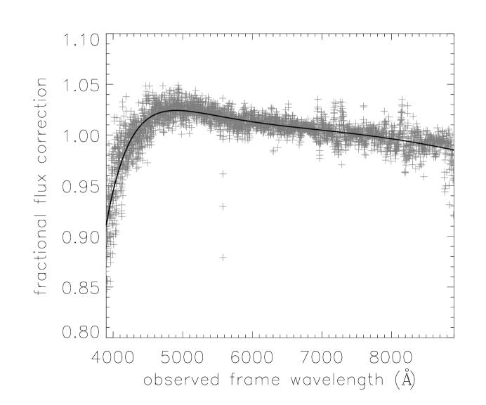
Figure 1.— The calibration spectrum (gray crosses) of the spectroscopic plate 390 and its 5th-order polynomial fit (black line). The correction in flux density between two epochs is a function of the observed-frame wavelength.

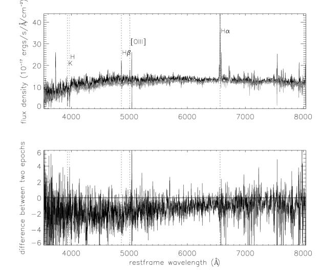
Figure 2.— An example star-forming galaxy without any calibration refinement ($F_{\mathrm{var}}=0.058$). Top: spectra at the first (black) and the second (gray) epoch. Bottom: difference spectrum.

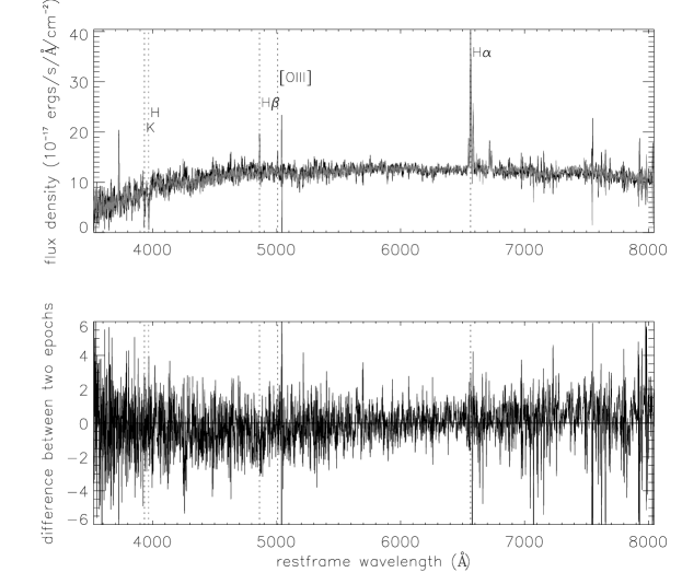
Figure 3.— The same galaxy as in Fig. 2, which shows zero continuum variability ($F_{\mathrm{var}}=0$) after the SYS+BAND calibration refinement. Top: spectra at the first (black) and the second (gray) epoch. Bottom: difference spectrum.

Figure 4.— $F_{\mathrm{var}}$ vs. S/N of galaxy spectra before (left) and after (right) the SYS+BAND calibration refinement. The number of objects in each spectroscopic plate is listed in Table LABEL:tab:plate.

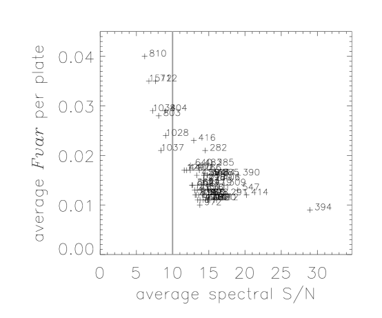
Figure 5.— The average variability of galaxy spectra over a given spectroscopic plate plotted versus the average spectral S/N. The spectra at S/N $\geq 10$ are selected in the subsequent definition of variable and non-variable candidates to minimize variation in $F_{\mathrm{var}}$ among plates.

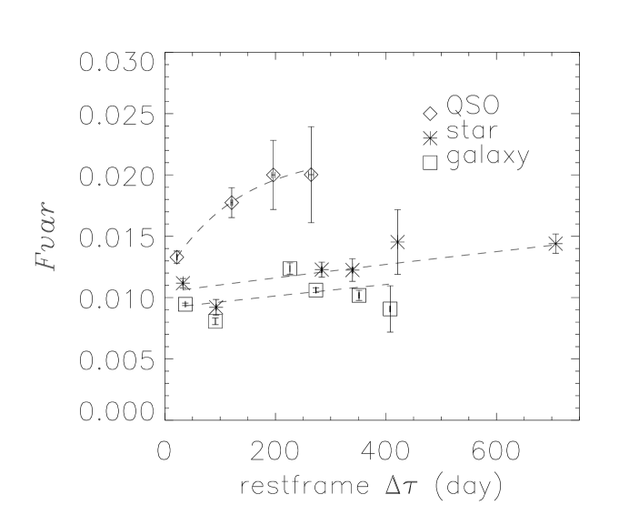
Figure 6.— Restframe structure function of the QSOs, stars and galaxies. Only spectra with S/N $\geq 10$ are shown. Error bar is 1$\sigma_{m}$ for each axis. Dotted line shows the best-fit structure function of an exponential functional form in $\Delta\tau_{\mathrm{r}est}$.

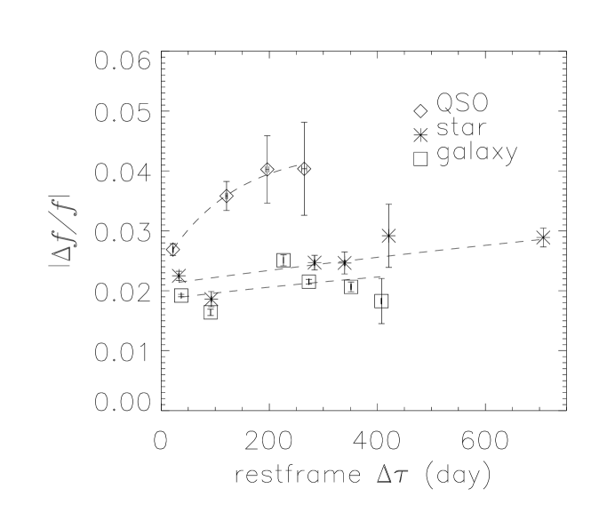
Figure 7.— Restframe structure function. Same as Fig. 6 except that the fraction change in total flux $|$$\Delta{f}/{f}$$|$  is used instead of $F_{\mathrm{var}}$.

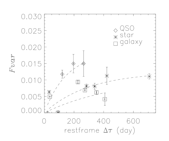
Figure 8.— Restframe structure function of the QSOs, stars and galaxies. Different from Fig. 6 which shows the total variability, here the variability at the zero time lag is quadrature subtracted, respectively in each spectral type. Only spectra with S/N $\geq 10$ are shown. Error bar is 1$\sigma_{m}$ for each axis. Dotted line shows the best-fit structure function of an exponential functional form in $\Delta\tau_{\mathrm{r}est}$.

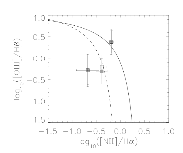
Figure 9.— The BPT diagram of the continuum variable candidates. The object type from the lowest to the highest [N II]/H$\alpha$ value is: star-forming, composite and Seyfert 2. In each duo the filled square represents the average line ratios of the brighter objects, and the empty square for the dimmer ones. The solid and dashed lines respectively define the Seyfert 2 and star-forming galaxies as given by Kewley et al. (2006). The line ratios in all object types do not show substantial change between both epochs. The error bar represents the $1\sigma$ sample scatter in each phase.

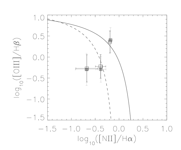
Figure 10.— Similar to Fig. 9, but in each duo the filled square represents the average line ratios of the first epoch, and the empty square for the latter epoch. The error bar represents the $1\sigma$ sample scatter in each epoch.

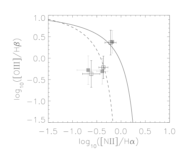
Figure 11.— Similar to Fig. 9, but in each duo the filled square represents the average line ratios of the continuum variable candidates, and the empty square for the non-variable ones. Line ratios in both cases are from the bright phase. The error bar represents the $1\sigma$ sample scatter.

Table 1Spectroscopic plates used in the analysis of galaxies.

plate	first epoch MJD	second epoch MJD	difference in MJD	total number of pair	number of pair
266	51602	51630	28	447	356
279	51608	51984	376	430	361
282	51630	51658	28	346	278
284	51662	51943	281	425	336
285	51663	51930	267	417	317
291	51660	51928	268	444	344
296	51665	51984	319	448	364
297	51663	51959	296	453	369
300	51666	51943	277	386	288
301	51641	51942	301	370	282
304	51609	51957	348	398	317
306	51637	51690	53	435	352
309	51666	51994	328	371	287
340	51691	51990	299	385	302
348	51671	51696	25	313	240
351	51695	51780	85	395	311
385	51783	51877	94	326	259
390	51816	51900	84	392	313
394	51812	51913	101	347	267
404	51812	51877	65	421	335
406	51817	52238	421	319	239
410	51816	51877	61	309	243
411	51817	51873	56	398	318
412	51931	52258	327	396	306
413	51821	51929	108	351	274
414	51869	51901	32	383	299
415	51810	51879	69	366	277
416	51811	51885	74	332	259
418	51817	51884	67	367	285
419	51812	51879	67	355	293
422	51811	51878	67	465	375
425	51884	51898	14	370	290
437	51869	51876	7	304	235
440	51885	51912	27	425	331
483	51902	51942	40	324	247
547	51959	52207	248	347	288
588	52029	52045	16	435	344
594	52027	52045	18	355	285
616	52374	52442	68	450	349
640	52178	52200	22	405	323
644	52149	52173	24	408	339
662	52147	52178	31	455	358
712	52179	52199	20	216	131
790	52433	52441	8	402	323
803	52264	52318	54	430	355
804	52266	52286	20	422	354
810	52326	52672	346	502	360
814	52370	52443	73	363	279
820	52433	52438	5	307	242
960	52425	52466	41	427	354
972	52428	52435	7	417	345
978	52431	52441	10	328	262
1028	52562	52884	322	466	371
1034	52525	52813	288	471	385
1037	52826	52878	52	508	417
1291	52735	52738	3	421	337
1512	53035	53742	707	144	99
1782	53299	53383	84	457	373
2009	53857	53904	47	449	354
2351	53772	53786	14	332	259
$\cdots$	$\cdots$	$\cdots$	$\cdots$	23,330	18,435

Table 2Statistics of $F_{\mathrm{var}}$ in galaxies using different calibration refinements.

method	mean	$\sigma_{m}$	$\sigma$
No refinement	0.020	0.0002	0.025
SYS+BAND	0.010	0.0001	0.009
SYS+BAND (280 km s-1)	0.012	0.0001	0.011
SYS+OIII	0.016	0.0001	0.015
SYS+BAND (RED galaxies)	0.010	0.0001	0.009
SYS+BAND (BLUE galaxies)	0.010	0.0001	0.009

Table 3Upper percentile of the galaxy variable candidates.

lower S/N	0	5	10	15	20
upper S/N	5	10	15	20	40
number	11	102	246	206	86
percentile	1.53	1.89	3.92	6.26	3.44

Table 4Statistics of $F_{\mathrm{var}}$ in the full galaxy sample.

type	number	mean	$\sigma_{m}$	$\sigma$
Seyfert 2	92	0.009	0.0008	0.008
Starforming	1333	0.012	0.0003	0.011
Composite	314	0.010	0.0005	0.009
eClass A	729	0.010	0.0004	0.010
eClass B	919	0.010	0.0003	0.010
eClass C	587	0.011	0.0004	0.010
eClass D	483	0.012	0.0005	0.010
eClass E	3	0.024	0.0100	0.017
eClass F	5	0.044	0.0124	0.028
RED	9603	0.009	0.0001	0.009
BLUE	2705	0.012	0.0002	0.011

Table 5Statistics of $F_{\mathrm{var}}$ in the galaxy variable candidates.

type	number	mean	$\sigma_{m}$	$\sigma$
Seyfert 2	5	0.026	0.0030	0.007
Starforming	62	0.037	0.0023	0.018
Composite	13	0.031	0.0043	0.015
eClass A	34	0.031	0.0027	0.016
eClass B	45	0.031	0.0020	0.014
eClass C	37	0.030	0.0015	0.009
eClass D	18	0.034	0.0030	0.013
RED	388	0.028	0.0006	0.012
BLUE	154	0.034	0.0012	0.015

Table 6Difference in AB synthetic absolute magnitude between the dim and bright phases in $g,r,i$ bands, for variable candidates.

type	$\left<M_{g}\right>$	$\left<M_{r}\right>$	$\left<M_{i}\right>$	$\left<z\right>$	$\left<\Delta{M_{g}}\right>$	$\left<\Delta{M_{r}}\right>$	$\left<\Delta{M_{i}}\right>$	$\delta(\left<\Delta{M_{g}}\right>)$	$\delta(\left<\Delta{M_{r}}\right>)$	$\delta(\left<\Delta{M_{i}}\right>)$	$\sigma(\Delta{M_{g}})$	$\sigma(\Delta{M_{r}})$	$\sigma(\Delta{M_{i}})$
Seyfert 2	-20.57	-21.36	-21.30	0.14	0.07	0.05	0.05	0.26	0.12	0.20	0.01	0.03	0.03
Starforming	-18.79	-19.37	-19.46	0.09	0.10	0.05	0.05	0.09	0.04	0.08	0.05	0.03	0.05
Composite	-19.79	-20.53	-20.53	0.11	0.09	0.04	0.03	0.19	0.08	0.13	0.05	0.02	0.03
eClass A	-20.70	-21.55	-21.25	0.15	0.08	0.05	0.06	0.11	0.05	0.85	0.04	0.04	0.05
eClass B	-20.12	-20.95	-20.74	0.13	0.09	0.05	0.04	0.10	0.04	4.82	0.03	0.03	0.03
eClass C	-19.95	-20.73	-20.81	0.12	0.09	0.04	0.04	0.12	0.05	0.08	0.03	0.02	0.03
eClass D	-18.18	-18.75	-18.91	0.07	0.09	0.04	0.06	0.16	0.07	0.12	0.05	0.02	0.06
RED	-20.14	-20.99	-20.91	0.13	0.08	0.04	0.05	0.03	0.01	3.16	0.04	0.03	0.04
BLUE	-19.27	-19.87	-19.89	0.10	0.09	0.05	0.05	0.06	0.03	0.05	0.05	0.03	0.05

Table 7Best-fit characteristic variability time scale.

type	zero-point $F_{\mathrm{var}}$	$\tau_{s}$ (year)	asymptotic $F_{\mathrm{var}}$($\Delta\tau_{\mathrm{r}est}$$\rightarrow\infty$)	reduced $\chi^{2}$	range in $\Delta\tau_{\mathrm{r}est}$ (day)
QSO	$0.012\pm 0.003$	$0.4\pm 1.0$	$0.022\pm 0.002$	$0.04$	$0-300$
star	$0.010\pm 0.069$	$11.2\pm 6.3$	$0.035\pm 0.035$	$3.41$	$0-710$
galaxy	$0.009\pm 0.162$	$8.5\pm 1.6$	$0.025\pm 0.081$	$19.52$	$0-500$

Table 8Best-fit characteristic variability time scale, after quadtrature subtraction of variability at zero time lag.

type	$\tau_{s}$ (year)	asymptotic $F_{\mathrm{var}}$($\Delta\tau_{\mathrm{r}est}$$\rightarrow\infty$)	reduced $\chi^{2}$	range in $\Delta\tau_{\mathrm{r}est}$ (day)
QSO	$0.4\pm 0.0$	$0.018\pm 0.005$	$13.10$	$0-300$
star	$0.8\pm 0.0$	$0.012\pm 0.003$	$49.71$	$0-710$
galaxy	$1.4\pm 0.0$	$0.011\pm 0.018$	$501.97$	$0-500$

Table 9BPT line-ratio difference between dim and bright phases, for variable candidates.

type	$\left<\right.$$\Delta$$\log_{10}$($[$N II$]$/H$\alpha$)$\left.\right>$	$\left<\right.$$\Delta$$\log_{10}$($[$O III$]$/H$\beta$)$\left.\right>$	$\sigma$($\Delta$$\log_{10}$($[$N II$]$/H$\alpha$))	$\sigma$($\Delta$$\log_{10}$($[$O III$]$/H$\beta$))
Seyfert 2	$0.02\pm 0.03$	$0.06\pm 0.08$	0.03	0.03
Starforming	$0.09\pm 0.01$	$0.16\pm 0.03$	0.17	0.21
Composite	$0.03\pm 0.03$	$0.11\pm 0.09$	0.03	0.08
eClass C	$0.17\pm 0.05$	$0.47\pm 0.12$	0.18	0.43
eClass D	$0.07\pm 0.02$	$0.15\pm 0.06$	0.08	0.17

Table 10Statistics of $F_{\mathrm{var}}$ in stars.

method	mean	$\sigma_{m}$	$\sigma$
No refinement	0.035	0.0011	0.053
SYS+BAND	0.012	0.0003	0.013

Table 11Statistics of $F_{\mathrm{var}}$ in QSOs.

method	mean	$\sigma_{m}$	$\sigma$
No refinement	0.036	0.0012	0.034
SYS+BAND	0.015	0.0005	0.014

Table 12Matched objects between GCVS and our samples.

RA (degree)	DEC (degree)	specClass	S/N	$\Delta\tau$	difference in $g$	difference in $r$	difference in $i$	$F_{\mathrm{var}}$	nSigma
218.750940	-0.768439	1	20.4	53	$0.13\pm 0.49$	$-0.05\pm 0.30$	$-0.09\pm 0.41$	0.017	1
118.540000	42.817851	1	39.0	7	$-0.02\pm 0.26$	$0.00\pm 0.16$	$0.00\pm 0.21$	0.005	0
119.352760	43.207637	1	43.0	7	$0.05\pm 0.23$	$0.01\pm 0.16$	$-0.02\pm 0.22$	0.011	3
120.915900	42.512477	1	46.5	7	$-0.23\pm 0.20$	$-0.03\pm 0.13$	$0.08\pm 0.18$	0.051	4
133.434070	57.811289	1	52.2	40	$0.16\pm 0.18$	$0.06\pm 0.12$	$0.00\pm 0.18$	0.045	4

Table 13Matched objects between SDSS Stripe 82 variable catalog and stars in this work.

RA (degree)	DEC (degree)	specClass	S/N	number of obs in $r$	$\Delta\tau$	difference in $g$	difference in $r$	difference in $i$	$F_{\mathrm{var}}$	nSigma
356.032540	1.027191	1	18.2	10	94	$0.03\pm 1.64$	$0.01\pm 0.45$	$0.00\pm 0.49$	0.003	0
356.151320	0.303432	1	9.1	12	94	$-0.01\pm 2.13$	$-0.02\pm 0.68$	$-0.04\pm 0.73$	0.007	0
356.171110	-1.220269	1	26.8	10	94	$0.08\pm 0.53$	$0.00\pm 0.28$	$-0.07\pm 0.37$	0.006	0
354.635580	0.856453	1	7.9	10	94	$0.02\pm 1.28$	$-0.02\pm 0.94$	$-0.09\pm 1.68$	0.039	1
12.348661	-0.299891	1	52.6	8	101	$0.01\pm 0.23$	$0.00\pm 0.15$	$0.00\pm 0.23$	0.000	0
13.369355	-0.722569	1	45.5	8	101	$-0.13\pm 0.35$	$0.01\pm 0.19$	$0.05\pm 0.27$	0.025	1
31.675864	0.988745	1	17.0	14	65	$-0.01\pm 0.60$	$0.00\pm 0.35$	$0.01\pm 0.53$	0.001	0
36.891406	0.437566	1	11.7	14	421	$0.03\pm 0.79$	$0.03\pm 0.58$	$0.02\pm 0.97$	0.013	0
35.787734	0.959517	1	25.6	14	421	$-0.06\pm 0.44$	$-0.03\pm 0.26$	$0.01\pm 0.37$	0.015	2
36.347691	0.660534	1	20.4	13	421	$-0.04\pm 0.57$	$-0.03\pm 0.33$	$-0.03\pm 0.47$	0.015	2
44.620576	-0.609703	1	14.3	14	61	$0.18\pm 0.74$	$0.01\pm 0.45$	$-0.09\pm 0.71$	0.036	4
44.322878	0.785284	1	13.2	14	61	$-0.14\pm 0.73$	$-0.01\pm 0.44$	$0.06\pm 0.68$	0.031	4
46.057464	-1.220639	1	29.6	12	56	$-0.16\pm 0.32$	$-0.03\pm 0.20$	$0.07\pm 0.29$	0.032	4
48.387960	0.715234	1	17.0	14	108	$-0.07\pm 0.56$	$-0.02\pm 0.35$	$0.03\pm 0.58$	0.014	1
49.984166	-0.044137	1	8.6	14	108	$-0.12\pm 1.16$	$-0.01\pm 0.79$	$0.05\pm 1.39$	0.030	0
51.883714	0.064299	1	54.1	12	32	$-0.40\pm 0.19$	$-0.05\pm 0.12$	$0.15\pm 0.17$	0.085	4
52.295747	0.603985	1	20.9	12	32	$-0.08\pm 0.62$	$-0.01\pm 0.34$	$0.04\pm 0.49$	0.015	2
52.476904	0.389118	1	45.5	14	32	$0.02\pm 0.28$	$0.00\pm 0.17$	$0.00\pm 0.24$	0.006	0
51.602434	0.674580	1	45.2	14	20	$0.01\pm 0.24$	$0.01\pm 0.16$	$-0.04\pm 0.21$	0.007	4
43.924804	-0.542138	1	2.8	14	707	$-0.10\pm 4.41$	$0.15\pm 2.26$	$0.17\pm 3.21$	0.017	0
44.201206	0.013831	1	19.2	14	707	$-0.15\pm 1.10$	$-0.01\pm 0.30$	$0.03\pm 0.30$	0.011	0
44.918114	0.758511	1	6.3	12	707	$-0.14\pm 2.89$	$-0.17\pm 0.98$	$-0.28\pm 1.13$	0.100	2

Table 14Matched objects between SDSS Stripe 82 variable catalog and QSOs in this work

nSigma	number of objects	percentage
0	231	67.3
1	45	13.1
2	33	9.6
3	10	2.9
4	24	7.0

References

- Abazajian et al. (2003) Abazajian, K., et al. 2003, AJ, 126, 2081
- Adelman-McCarthy et al. (2008) Adelman-McCarthy, J. K., et al. 2008, ApJS, 175, 297
- Antonucci (1993) Antonucci, R. 1993, ARA&A, 31, 473
- Aretxaga et al. (1997) Aretxaga, I., Cid Fernandes, R., & Terlevich, R. J. 1997, MNRAS, 286, 271
- Baldwin et al. (1981) Baldwin, J. A., Phillips, M. M., & Terlevich, R. 1981, PASP, 93, 5
- Blanton et al. (2003) Blanton, M. R., Lin, H., Lupton, R. H., Maley, F. M., Young, N., Zehavi, I., & Loveday, J. 2003, AJ, 125, 2276
- Bonoli et al. (1979) Bonoli, F., Braccesi, A., Federici, L., Zitelli, V., & Formiggini, L. 1979, A&AS, 35, 391
- Bono et al. (2003) Bono, G., Trevese, D., & Turatto, M. 2003, Memorie della Societa Astronomica Italiana, 74, 1004
- Brunzendorf & Meusinger (2001) Brunzendorf, J., & Meusinger, H. 2001, A&A, 373, 38
- Bruzual & Charlot (2003) Bruzual, G., & Charlot, S. 2003, MNRAS, 344, 1000
- Connolly et al. (1995) Connolly, A. J., Szalay, A. S., Bershady, M. A., Kinney, A. L., & Calzetti, D. 1995, AJ, 110, 1071
- Cristiani et al. (1996) Cristiani, S., Trentini, S., La Franca, F., Aretxaga, I., Andreani, P., Vio, R., & Gemmo, A. 1996, A&A, 306, 395
- de Vries et al. (2003) de Vries, W. H., Becker, R. H., & White, R. L. 2003, AJ, 126, 1217
- Dobos et al. (2006) Dobos, L., Budavari, T., Csabai, I., & Szalay, A. 2006, The Virtual Observatory in Action: New Science, New Technology, and Next Generation Facilities, 26th meeting of the IAU, Special Session 3, 17-18, 21-22 August, 2006 in Prague, Czech Republic, SPS3, #76, 3
- Fukugita et al. (1996) Fukugita, M., Ichikawa, T., Gunn, J. E., Doi, M., Shimasaku, K., & Schneider, D. P. 1996, AJ, 111, 1748
- Giannuzzo & Stirpe (1996) Giannuzzo, E. M., & Stirpe, G. M. 1996, A&A, 314, 419
- Goodrich (1989) Goodrich, R. W. 1989, ApJ, 340, 190
- Guainazzi et al. (1998) Guainazzi, M., Matt, G., Antonelli, L. A., Fiore, F., Piro, L., & Ueno, S. 1998, MNRAS, 298, 824
- Gunn et al. (1998) Gunn, J. E., et al. 1998, AJ, 116, 3040
- Gunn et al. (2006) Gunn, J. E., et al. 2006, AJ, 131, 2332
- Hao et al. (2005) Hao, L., et al. 2005, AJ, 129, 1783
- Hawkins (1993) Hawkins, M. R. S. 1993, Nature, 366, 242
- Heckman (1980) Heckman, T. M. 1980, A&A, 87, 152
- Hogg et al. (2001) Hogg, D. W., Finkbeiner, D. P., Schlegel, D. J., & Gunn, J. E. 2001, AJ, 122, 2129
- Hopkins et al. (2003) Hopkins, A. M., et al. 2003, ApJ, 599, 971
- Hughes et al. (1992) Hughes, P. A., Aller, H. D., & Aller, M. F. 1992, ApJ, 396, 469
- Ivezić et al. (2003) Ivezić, Ž., et al. 2003, Memorie della Societa Astronomica Italiana, 74, 978
- Ivezić et al. (2004) Ivezić, Ž., et al. 2004, Astronomische Nachrichten, 325, 583
- Ivezić et al. (2004) Ivezić, Ž., et al. 2004, The Interplay Among Black Holes, Stars and ISM in Galactic Nuclei, 222, 525
- Jang (2001) Jang, M. 2001, Ap&SS, 275, 209
- Kauffmann et al. (2003) Kauffmann, G., et al. 2003, MNRAS, 346, 1055
- Kawaguchi et al. (1998) Kawaguchi, T., Mineshige, S., Umemura, M., & Turner, E. L. 1998, ApJ, 504, 671
- Kennicutt (1992) Kennicutt, R. C., Jr. 1992, ApJS, 79, 255
- Kewley et al. (2006) Kewley, L. J., Groves, B., Kauffmann, G., & Heckman, T. 2006, MNRAS, 372, 961
- Kholopov et al. (1999) Kholopov, P. N., et al. 1999, VizieR Online Data Catalog, 2214, 0
- Komossa (2008) Komossa, S. 2008, Revista Mexicana de Astronomia y Astrofisica Conference Series, 32, 86
- Lawson & Hanson (1974) Lawson, C. L. and Hanson, R. J., Solving Least Square Problem 1974, Prentice-Hall
- Lupton et al. (2001) Lupton, R., Gunn, J. E., Ivezić, Z., Knapp, G. R., & Kent, S. 2001, Astronomical Data Analysis Software and Systems X, 238, 269
- Madgwick et al. (2003) Madgwick, D. S., Somerville, R., Lahav, O., & Ellis, R. 2003, MNRAS, 343, 871
- Mateos et al. (2007) Mateos, S., Barcons, X., Carrera, F. J., Page, M. J., Ceballos, M. T., Hasinger, G., & Fabian, A. C. 2007, A&A, 473, 105
- Meusinger & Brunzendorf (2002) Meusinger, H., & Brunzendorf, J. 2002, A&A, 390, 439
- Miller et al. (2003) Miller, C. J., Nichol, R. C., Gómez, P. L., Hopkins, A. M., & Bernardi, M. 2003, ApJ, 597, 142
- Mueller et al. (2003) Mueller, M., Madejski, G. M., Done, C., & Zycki, P. T. 2003, Bulletin of the American Astronomical Society, 35, 637
- O’Donnell (1994) O’Donnell, J. E. 1994, ApJ, 422, 158
- Oke & Gunn (1983) Oke, J. B., & Gunn, J. E. 1983, ApJ, 266, 713
- Osterbrock (1989) Osterbrock, D. E. 1989, Astrophysics of gaseous nebulae and active galactic nuclei, University Science Books, 1989
- Osterbrock & Pogge (1985) Osterbrock, D. E., & Pogge, R. W. 1985, ApJ, 297, 166
- Pereyra et al. (2006) Pereyra, N. A., Vanden Berk, D. E., Turnshek, D. A., Hillier, D. J., Wilhite, B. C., Kron, R. G., Schneider, D. P., & Brinkmann, J. 2006, ApJ, 642, 87
- Peterson et al. (1995) Peterson, B. M., Pogge, R. W., Wanders, I., Smith, S. M., & Romanishin, W. 1995, PASP, 107, 579
- Peterson et al. (1998) Peterson, B. M., Wanders, I., Bertram, R., Hunley, J. F., Pogge, R. W., & Wagner, R. M. 1998, ApJ, 501, 82
- Peterson et al. (2000) Peterson, B. M., McHardy, I. M., & Wilkes, B. J. 2000, New Astronomy Review, 44, 491
- Peterson (2001) Peterson, B. M. 2001, Advanced Lectures on the Starburst-AGN , 3
- Pier et al. (2003) Pier, J. R., Munn, J. A., Hindsley, R. B., Hennessy, G. S., Kent, S. M., Lupton, R. H., & Ivezić, Ž. 2003, AJ, 125, 1559
- Richards et al. (2002) Richards, G. T., et al. 2002, AJ, 123, 2945
- Rodriguez-Pascual et al. (1997) Rodriguez-Pascual, P. M., et al. 1997, ApJS, 110, 9
- Schlegel et al. (1998) Schlegel, D. J., Finkbeiner, D. P., & Davis, M. 1998, ApJ, 500, 525
- Sesar et al. (2006) Sesar, B., et al. 2006, AJ, 131, 2801
- Sesar et al. (2007) Sesar, B., et al. 2007, AJ, 134, 2236
- Simonetti et al. (1985) Simonetti, J. H., Cordes, J. M., & Heeschen, D. S. 1985, ApJ, 296, 46
- Smith et al. (2002) Smith, J. A., et al. 2002, AJ, 123, 2121
- Spitzer (1978) Spitzer, L. 1978, New York Wiley-Interscience, 1978. 333
- Stalin et al. (2004) Stalin, C. S., Gopal-Krishna, Sagar, R., & Wiita, P. J. 2004, MNRAS, 350, 175
- Stoughton et al. (2002) Stoughton, C., et al. 2002, AJ, 123, 485
- Strauss et al. (2002) Strauss, M. A., et al. 2002, AJ, 124, 1810
- SubbaRao et al. (2002) SubbaRao, M., Frieman, J., Bernardi, M., Loveday, J., Nichol, B., Castander, F., & Meiksin, A. 2002, Proc. SPIE, 4847, 452
- Tohline & Osterbrock (1976) Tohline, J. E., & Osterbrock, D. E. 1976, ApJ, 210, L117
- Trevese et al. (1994) Trevese, D., Kron, R. G., Majewski, S. R., Bershady, M. A., & Koo, D. C. 1994, ApJ, 433, 494
- Trippe et al. (2008) Trippe, M. L., Crenshaw, D. M., Deo, R., & Dietrich, M. 2008, AJ, 135, 2048
- Tucker et al. (2006) Tucker, D. L., et al. 2006, Astronomische Nachrichten, 327, 821
- Urry & Padovani (1995) Urry, C. M., & Padovani, P. 1995, PASP, 107, 803
- Vanden Berk et al. (2001) Vanden Berk, D. E., et al. 2001, AJ, 122, 549
- Vanden Berk et al. (2004) Vanden Berk, D. E., et al. 2004, ApJ, 601, 692
- Vaughan et al. (2003) Vaughan, S., Edelson, R., Warwick, R. S., & Uttley, P. 2003, MNRAS, 345, 1271
- Veilleux & Osterbrock (1987) Veilleux, S., & Osterbrock, D. E. 1987, ApJS, 63, 295
- Veilleux et al. (1995) Veilleux, S., Kim, D.-C., Sanders, D. B., Mazzarella, J. M., & Soifer, B. T. 1995, ApJS, 98, 171
- Wanders et al. (1992) Wanders, I., Peterson, B. M., Pogge, R. W., Derobertis, M. M., & van Groningen, E. 1992, A&A, 266, 72
- Wang & Wei (2008) Wang, J., & Wei, J. Y. 2008, ApJ, 679, 86
- Wilhite et al. (2005) Wilhite, B. C., Vanden Berk, D. E., Kron, R. G., Schneider, D. P., Pereyra, N., Brunner, R. J., Richards, G. T., & Brinkmann, J. V. 2005, ApJ, 633, 638
- Wilhite et al. (2006) Wilhite, B. C., Vanden Berk, D. E., Brunner, R. J., & Brinkmann, J. V. 2006, ApJ, 641, 78
- Winkler et al. (1992) Winkler, H., Glass, I. S., van Wyk, F., Marang, F., Jones, J. H. S., Buckley, D. A. H., & Sekiguchi, K. 1992, MNRAS, 257, 659
- Yip et al. (2004) Yip, C. W., et al. 2004, AJ, 128, 585
- York et al. (2000) York, D. G., et al. 2000, AJ, 120, 1579
- Zhou et al. (2006) Zhou, H., Wang, T., Yuan, W., Lu, H., Dong, X., Wang, J., & Lu, Y. 2006, ApJS, 166, 128