A Simple Intrinsic Reduced-Observer for Geodesic Flow

Abstract

Aghannan and Rouchon proposed a new design method of asymptotic observers for a class of nonlinear mechanical systems: Lagrangian systems with configuration (position) measurements. The (position and velocity) observer is based on the Riemannian structure of the configuration manifold endowed with the kinetic energy metric and is intrinsic. They proved local convergence. When the system is conservative, we propose an intrinsic reduced order (velocity) observer based on the Jacobi metric, which can be initialized such that it converges exponentially for any initial true velocity. For non-conservative systems the observer can be used as a complement to the one of Aghannan and Rouchon. More generally the reduced observer provides velocity estimation for geodesic flow with position measurements. Thus it can be (formally) used as a fluid flow soft sensor in the case of a perfect incompressible fluid. When the curvature is negative in all planes the geodesic flow is sensitive to initial conditions. Surprisingly in this case we have global exponential convergence and the more unstable the flow is, faster is the convergence.

Keywords

Riemannian curvature, geodesic flow, non-linear asymptotic observer, Lagrangian mechanical systems, intrinsic equations, contraction, infinite dimensional Lie group, incompressible fluid.

There is no general method to design asymptotic observers for observable non-linear systems. Indeed only some specific types of linearities have been tackled in the literature. In particular over the last few years some work has been devoted to observer design for systems possessing symmetries. [2, 7, 14, 9] consider a finite-dimensional group of symmetries acting on the state space, and [8] a left-invariant dynamics on a Lie group. Symmetries generally correspond to invariance to some changes of units and frame. Invariance to any change of coordinates was raised by [3] who designed an intrinsic observer for a class of non-linear systems: Lagrangian systems with position (configuration) measurements. The aim is to estimate the velocity, independently from any nontrivial choice of coordinates, and of course never differentiate the (noisy) output. The observer was adapted to the specific case of a left-invariant system on a Lie group by [15]. Observer [3] is based on the Riemannian structure of the configuration manifold endowed with the kinetic energy metric. This geometry had already been used in control theory of mechanical systems (see e.g. [11, 10]). The convergence of the observer is local.

According to the Maupertuis principle, the motion of a conservative Lagrangian system is a geodesic flow (motion along a geodesic with constant speed) for the Jacobi metric, intrinsically defined using the kinetic and potential energies, up to a time reparametrization. In this paper we consider the general problem of building a reduced order velocity observer for geodesic flow on a Riemannian manifold with position measurements. A reduced observer is meant to estimate only the unmeasured part of the system’s state (here the velocity). Under some basic assumptions relative to the injectivity radius (also formulated in [3]) we have the following results (Theorem 1). If there is an upper bound $A>0$ on the sectional curvature in all planes, choosing $\hat{v}(0)=0$, the reduced velocity observer always converges exponentially to the true velocity, as long as the gain is larger than a linear function of $\sqrt{A}$. Unfortunately the higher the gain is the most sensitive to noise the observer is. An even better situation occurs when the sectional curvature is non-positive in all planes: the reduced observer is globally exponentially convergent for all positive gain. In fact, the more negative the curvature is the faster the observer converges. This feature is surprising enough as negative curvature implies exponential divergence between two nearby geodesics, and thus “amplifies” initial errors. This is a major difference with [3] who used additional terms precisely to cancel the effects of (negative) curvature.

For mechanical Lagrangian systems the observer of Aghannan and Rouchon is only locally convergent. In the absence of external forces the reduced observer provides an alternative observer which allows to always estimate the true velocity. When there are external forces, the reduced-observer can be used as a complement to [3]. The gain must be chosen large enough, so that the reduced observer converges before the energy varies significantly. If so, it provides an estimated velocity close to the true one, with which the observer [3] can be initialized.

The reduced observer is also applied, formally, to a basic velocimetry problem: compute the velocity of a perfect incompressible fluid observing the fluid particles. The principle of least action implies that the motion of an incompressible fluid can be viewed as a geometric flow. We consider the case of a two-dimensional fluid. As the convergence properties of the observer depend on the sign of the curvature, we will use results and heuristics of Arnol’d [5]. Following them, we show that global convergence could be expected for a large class of trajectories, since the curvature is positive only in a few sections. This latter fact also implies instability of the flow, and Arnol’d interpretes the difficulty of weather’s prediction as a consequence of this result. Note that the problem tackled is nontrivial, as the system is nonlinear, infinite dimensional, and possibly sensitive to initial conditions.

In Section I we give the general motivations introducing Lagrangian systems on manifolds and Maupertuis’ principle. In Section II we introduce the observer. In Section III we consider applications to some mechanical and hydrodynamical systems. In Section IV the convergence in the case of positive constant curvature is illustrated by simulations on the sphere.

1 Lagrangian systems on manifolds

Consider the classical mechanical system with $n$ degrees of freedom described by the Lagrangian

$$\mathcal{L}(q,\dot{q})=\frac{1}{2}g_{ij}(q)\dot{q}^{i}\dot{q}^{j}-U(q)$$

where the generalized positions $q\in\mathcal{M}$ are written in the local coordinates $(q^{i})_{i=1...n}$, $g(q)=(g_{ij}(q))_{i=1\ldots n,j=1\ldots n}$ is a Riemaniann metric on the configuration space $\mathcal{M}$, and $U:\mathcal{M}\mapsto{\mathbb{R}}$ is the potential energy. The Euler-Lagrange equations write in the local coordinates

$${\frac{d}{dt}}\left(\frac{\partial}{\partial\dot{q}^{i}}\mathcal{L}\right)=\frac{\partial}{\partial q^{i}}\mathcal{L},\quad i=1,...,n$$ (1)

One can prove using $\frac{\partial g^{ik}}{\partial q^{l}}g_{jk}=-g^{ik}\frac{\partial g_{jk}}{\partial q^{l}}$ where $g^{il}$ are components of $g^{-1}$ that (1) writes

$$\begin{array}[]{rl}\ddot{q}^{i}&=-\Gamma^{i}_{jk}(q)\dot{q}^{j}\dot{q}^{k}+\frac{\partial}{\partial q^{i}}U\end{array}$$ (3)

where the Christoffel symbols $\Gamma^{i}_{jk}$ are given by $\Gamma^{i}_{jk}=\frac{1}{2}g^{il}\left(\frac{\partial g_{lk}}{\partial q^{j}}+\frac{\partial g_{jl}}{\partial q^{k}}-\frac{\partial g_{jk}}{\partial q^{l}}\right)$ (see e.g. [1]) . A curve $\gamma(t)$ which is a critical point of the action

$$S(\gamma)=\int_{0}^{T}L(\gamma(t),\dot{\gamma}(t)dt)$$

among all curves with fixed endpoints satisfies the Euler-Lagrange equations (1).

1.1 Lagrangian system in a potential field

Consider a conservative Lagrangian system evolving in an admissible region $\{q\in\mathcal{M}:U(q)<E\}$. The energy of the system $E=T(q,\dot{q})+U(q)=\frac{1}{2}g_{ij}(q)\dot{q}^{i}\dot{q}^{j}+U(q)$ is fixed. According to the Maupertuis principle of least action (see e.g. [5]), in the Riemannian geometry defined by the Jacobi metric $\hat{g}^{ij}(q)=2(E-U(q))g^{ij}(q)$ and the natural parameter $\tau$ such that $\frac{d\tau}{dt}=2(E-U(q(t)))$, the geodesic flow is a solution of the equation of motion (3). Indeed if the $\hat{\Gamma}^{i}_{jk}$ are the Christoffel symbols associated to the metric $\hat{g}$ we have

$$\frac{d^{2}}{d\tau^{2}}{q}^{i}+\hat{\Gamma}^{i}_{jk}(q)\frac{d}{d\tau}{q}^{j}\frac{d}{d\tau}{q}^{k}=0$$ (4)

which writes intrinsically $\hat{\nabla}_{\frac{dq}{d\tau}}\frac{dq}{d\tau}=0$ and defines the geodesic flow ($\hat{\nabla}$ is the Levi-Civita covariant differentiation of the Jacobi metric).

1.2 Geodesic flow and holonomic constraints

A material particle constrained to lie on a manifold moves along a geodesic [5]. Indeed $E=T$, $\hat{g}=2Eg$, $d\tau=2Edt$ ensure the energy $T$ is fixed. According to Maupertuis’ principle the motion minimizes $\int_{\gamma}\sqrt{\hat{g}_{ij}\frac{d}{d\tau}{q}^{i}\frac{d}{d\tau}{q}^{j}}d\tau=(1/{\sqrt{2E}})\int_{\gamma}\sqrt{g_{ij}\frac{d}{dt}{q}^{i}\frac{d}{dt}{q}^{j}}dt$ which is proportional to the geodesic length in the metric $g$. More generally an inertial motion of a Lagrangian system with $k$ holonomic constraints can be viewed as the inertial motion of a particle constrained to lie on a submanifold of dimension $n-k$ (see e.g. [5] p 90). A conservative Lagrangian system in a potential field with holonomic constraints satisfies the Maupertuis’ principle on the configuration submanifold of dimension $n-k$.

2 An intrinsic reduced-observer

Let us build an observer to estimate the velocity $\dot{q}$ of a point $q$ moving along the geodesics of ${\mathcal{M}}$ with constant speed, when the position $q$ is measured (with noise). First suppose $\mathcal{M}=\mathbb{R}^{n}$ endowed with Euclidian metric. Let $\dot{q}=v$ and $\dot{v}=0$. For such a linear system a Luenberger reduced dimension observer with arbitrary dynamics can be constructed [13]. The goal is to estimate only the part of the state that is not directly measured. An auxiliary variable $\xi$, which is a combination between the unmeasured part of the state and the output, is generally introduced:

$$\xi=q-\lambda v\qquad(\text{and~{}thus}~{}~{}\dot{\xi}=v)$$ (5)

To estimate $\xi$ and $\dot{\xi}$ consider the reduced observer:

$${\frac{d}{dt}}\hat{\xi}=-\frac{\hat{\xi}-q}{\lambda}$$ (6)

It can be interpreted as a simple pursuit algorithm with proportional feedback. Let $\hat{v}={\frac{d}{dt}}\hat{\xi}$. Let us prove $\hat{\xi}-\xi\rightarrow 0$ and $\hat{v}-v\rightarrow 0$. We have ${\frac{d}{dt}}{\hat{v}}=-(1/\lambda)(\hat{v}-v)$ implying $\hat{v}\rightarrow v$ for $\lambda>0$. As $\hat{\xi}=q-\lambda\hat{v}$, we have $\hat{\xi}-\xi\rightarrow 0$, and $\hat{\xi}$ is asymptotically moving behind $q$ at fixed distance $\lambda\lVert\dot{q}\rVert$. If $\mathcal{M}$ is any Riemannian manifold consider

$${\frac{d}{dt}}\hat{\xi}=-\frac{1}{2\lambda}~{}\overrightarrow{grad}_{\hat{\xi}}~{}D^{2}(\hat{\xi},q),\quad\lambda>0$$ (7)

where $D(\hat{\xi},q)$ is the geodesic distance between $\hat{\xi}$ and $q$. If $D(\hat{\xi},q)$ is smaller than the injectivity radius at $q$, then (7) means that ${\frac{d}{dt}}\hat{\xi}$ is a vector which is tangent to the geodesic linking $\hat{\xi}$ and $q$, and whose norm is proportional to $D(\hat{\xi},q)$. The dynamic does not depend on any choice of local coordinates in ${\mathbb{R}}^{n}$, and is a generalization of (6). We want to prove that $D(\hat{\xi},\xi)\rightarrow 0$ where $\xi$ is a point following $q$ at distance $\lambda\lVert\dot{q}\rVert$ on the geodesic $\{q(t):t>0\}$. The parallel transport $\mathcal{T}_{//\hat{\xi}\rightarrow q}$ of ${\frac{d}{dt}}\hat{\xi}$ to the tangent space at $q$ along the geodesic joining $\hat{\xi}$ and $q$ is an estimation of $v=\dot{q}$.

$$\hat{v}=\mathcal{T}_{//\hat{\xi}\rightarrow q}{\frac{d}{dt}}\hat{\xi}$$ (8)

Theorem 1.

Let ${\mathcal{M}}$ be a Riemannian manifold. Let $T<\infty$. Let $t\mapsto q(t)\in{\mathcal{M}}$ satisfy $\nabla_{\dot{q}}\dot{q}=0$ for $t\in[0,T]$. Let $\xi(t)=\exp_{q(t)}(-\lambda{\dot{q}})$. Consider the observer (7). Let (9) be the inequality

$$D(\hat{\xi}(t),\xi(t))\leq e^{-\frac{1}{\lambda}t}D(\hat{\xi}(0),\xi(0))\quad\forall t\in[0,T]$$ (9)

• Suppose the Riemannian curvature is non-positive in all planes. If for all $t\in[0,T]$, $D(\hat{\xi}(t),q(t))$ is bounded by the injectivity radius $I(t)$ at $q(t)$ (i.e. there exists a unique geodesic joining $\hat{\xi}$ and $q(t)$), (9) is true for all $\lambda>0$. When the manifold is complete and simply-connected (Hadamard manifold), the injectivity radius is infinite (Cartan-Hadamard theorem) and (9) is always true. In particular $\hat{\xi}(0)$ can be chosen arbitrarily. Moreover for all $t\in[0,T]$

  $$\lambda\lVert\hat{v}(t)-\dot{q}(t)\rVert\leq D(\hat{\xi}(t),\xi(t))\leq e^{-\frac{1}{\lambda}t}D(\hat{\xi}(0),\xi(0))$$ (10)

• Suppose the sectional curvature is bounded from above by $A>0$. (9) is true as long as the distance $D(\hat{\xi}(t),q(t))$ remains bounded by $\max(\frac{\pi}{4\sqrt{A}},I(t))$ for all $t\in[0,T]$. If the manifold is simply connected and ${\lambda}>\frac{\pi}{4\lVert\dot{q}\rVert_{g}\sqrt{A}}$, (9) is true as soon as $D(\hat{\xi}(0),q(0))<\frac{\pi}{4\sqrt{A}}.$ Moreover in this case we have exponential convergence in polar coordinates for all $t\in[0,T]$:

  $$\lambda|~{}\lVert\hat{v}(t)\rVert-\lVert\dot{q}\rVert~{}|\leq D(\hat{\xi}(t),\xi(t)),$$ (11)

  $$0\leq\sin(\alpha_{A}(t))\leq\frac{\sqrt{A}~{}}{\sin(\sqrt{A}~{}\lambda\lVert\dot{q}\rVert)}D(\hat{\xi}(t),\xi(t))$$

  where $\alpha_{A}(t)\rightarrow 0$ and the angle $\alpha(t)$ between $\hat{v}(t)$ and $\dot{q}(t)$ satisfies $0\leq\alpha(t)\leq\alpha_{A}(t)\leq\pi$.

The convergence (9) of the observer’s state variable $\hat{\xi}$ is not sufficient to prove that $\hat{v}$ converges. Indeed the estimated velocity $\hat{v}$ is linked to $\hat{\xi}$ via a non-linear geometric transformation. Yet geometry of triangles on curved surfaces will allow to prove (10) and (LABEL:speed:conv:eq2).

Proof.

The proof utilizes two differential geometry lemmas. Lemma 2 is a consequence of Synge’s lemma (see e.g. [19] p 316) for which a direct demonstration is proposed.

Lemma 1.

Let ${\mathcal{M}}$ be a smooth Riemannian manifold. Let $P\in{\mathcal{M}}$ be fixed. On the subspace of ${\mathcal{M}}$ defined by the injectivity radius at $P$ we consider

$${\frac{d}{dt}}x=-\frac{1}{2\lambda}~{}\overrightarrow{grad}_{x}~{}D^{2}(P,x)\quad\lambda>0$$ (12)

If the sectional curvature is non-positive in all planes, the dynamics is a contraction in the sense of [12], i.e, if $\delta x$ is a virtual displacement at fixed $t$ we have

$${\frac{d}{dt}}\|\delta x\|_{g}^{2}\leq-\frac{2}{\lambda}\|\delta x\|_{g}^{2}$$ (13)

where $\|~{}\|_{g}~{}$ is the norm associated to the metric $g$. If the sectional curvature in all planes is upper bounded from above by $A>0$, (13) holds for $D(P,x)<\pi/(4\sqrt{A})$.

Proof.

The virtual displacement is defined [12] as a linear tangent differential form, and can be viewed by duality as a vector of $TM|_{x}$. Let us define a surface $\Sigma$. Let $\gamma_{0}$ be the geodesic joining $P$ to $x$. Consider $x_{\epsilon}=\exp_{x}(\epsilon~{}\delta x)\in{\mathcal{M}}$. It is linked to $P$ by a geodesic, say $\gamma_{\epsilon}$. Up to second order terms in $\epsilon$ we have $\dot{\gamma}_{\epsilon}(0)-\dot{\gamma}_{0}(0)=\epsilon u$ where $u$ is a tangent vector at $P$. The directions defined by $\gamma_{0}$ and $u$ at $P$ span a 2-plane tangent at $P$. All the geodesics having a direction tangent to this 2-plane at $P$ span a smooth surface $\Sigma$ embedded in ${\mathcal{M}}$ which inherits the Riemannian metric $g$. We have $x\in\Sigma$ and $\delta x\in T_{x}\Sigma\subset T_{x}{\mathcal{M}}$. $\Sigma$ is invariant under the flow $\eqref{variete:dyn}$, as the gradient term is tangent to the geodesics heading towards $P$. Indeed, let $\gamma$ be parameterized by the arclength $\sigma$, and let $\sigma_{0}=D(P,x)$. The squared distance increases the most in the direction of the geodesics. Thus the gradient tangent to the geodesic. We have $D^{2}(P,\gamma(\sigma_{0}+\epsilon))=(\sigma_{0}+\epsilon)^{2}$. Up to second order terms $D^{2}(P,\gamma(\sigma_{0}+\epsilon))=D^{2}(P,x)+\epsilon\langle\overrightarrow{grad}_{x}~{}D^{2}(P,x),\frac{d\gamma}{d\sigma}(\sigma_{0})\rangle_{g}$. The norm of the gradient is thus is $2D(P,x)$.

Following [19] (p 177) we use specific coordinates on $\Sigma$ called “polar coordinates”. Let $e_{1},e_{2}$ be an euclidian frame of $T_{P}\Sigma$ for the inherited metric and $e_{1}$ be tangent to $\gamma_{0}$. We define $\Phi:(\sigma,\theta)\mapsto\exp_{P}(\sigma\cos\theta e_{1}+\sigma\sin\theta e_{2})$. $\Sigma$ is parameterized by $\sigma$, the geodesic length to $P$, and $\theta$, the angle in $T_{P}\Sigma$ with $e_{1}$. In the polar coordinates, the elementary length is given by

$$ds^{2}=d\sigma^{2}+G(\sigma,\theta)d\theta^{2}$$

and $G$ satisfies the initial conditions $\sqrt{G}=0$ and $\frac{\partial\sqrt{G}}{\partial\sigma}=1$ at $\sigma=0$. According to a classical result [19] the Gauss curvature at the point $u=\Phi(\sigma,\theta)$ is given by $K(\sigma,\theta)=\frac{-1}{\sqrt{G(\sigma,\theta)}}\frac{\partial^{2}\sqrt{G(\sigma,\theta)}}{\partial\sigma^{2}}$. We will prove (lemma 2) that the Gaussian curvature at $u=\Phi(\sigma,\theta)\in\Sigma$ is less than the sectional curvature in the tangent plane to $\Sigma$ at $u$: $K(\sigma,\theta)\leq K_{sec}(T_{u}\Sigma)$.

Suppose $K_{sec}(T_{u}\Sigma)\leq 0$. It implies $K(\sigma,\theta)\leq 0$. Along $\gamma$ we have

$$\frac{\partial^{2}G(\sigma,\theta)}{\partial\sigma^{2}} =\frac{\partial}{\partial\sigma}(2\sqrt{G(\sigma,\theta)}\frac{\partial\sqrt{G(\sigma,\theta)}}{\partial\sigma})$$ (14)

$$=2\left((\frac{\partial\sqrt{G(\sigma,\theta)}}{\partial\sigma})^{2}-G(\sigma,\theta)K(\sigma,\theta)\right)\geq 0$$

and thus $\frac{\partial}{\partial\sigma}(\sigma\frac{\partial G}{\partial\sigma})\geq\frac{\partial G}{\partial\sigma}$ which yields by integration $\sigma\frac{\partial G}{\partial\sigma}\geq G$ since $G(0,\theta)=0$. In the polar coordinates the dynamics (12) reads

$$\dot{\sigma}=-\frac{1}{\lambda}\sigma;\qquad\dot{\theta}=0$$

Indeed we already stated that the gradient is tangent to the geodesic, thus $\dot{\theta}=0$, and (12) becomes a one-dimensional dynamics along the geodesic, and as $D^{2}(P,x)=\sigma^{2}$ we have $\lVert\overrightarrow{grad}_{x}~{}D^{2}(x,P)\rVert_{g}=2\sigma$. Writing $\|\delta x\|^{2}=\alpha^{2}\delta\sigma^{2}+\beta^{2}G(\sigma,0)\delta\theta^{2}$ we have along the geodesic $\gamma_{0}$ (parameterized by $\sigma$ and $\theta=0$) the following inequality, proving (13).

$${\frac{d}{dt}}\|\delta x\|^{2}=-2\frac{\alpha^{2}}{\lambda}\delta\sigma^{2}-2\beta^{2}\frac{\sigma}{\lambda}\frac{\partial{G(\sigma,0)}}{\partial\sigma}\delta\theta^{2}\leq-\frac{2}{\lambda}\|\delta x\|^{2}$$ (15)

Suppose now $K_{sec}(T_{u}\Sigma)\leq A$. Let $z(\sigma)=\sqrt{G(\sigma,0)}$. We have $z^{\prime\prime}=-K(\sigma,0)z$, $z(0)=0,~{}z^{\prime}(0)=1$, with $K(\sigma,0)\leq A$. The Sturm comparison theorem allows to compare $z$ to the solution of equation $y^{\prime\prime}=-Ay$, $y(0)=0,~{}y^{\prime}(0)=1$, i.e. $y(\sigma)=\sin(\sqrt{A}\sigma)/\sqrt{A}$. A Taylor expansion in $0$ shows there exists $\mu>0$ such that $z(\sigma)/z^{\prime}(\sigma)<y(\sigma)/y^{\prime}(\sigma)$ for $0<\sigma\leq\mu$. It is proved in [4] (Sturm Comparison theorem) this implies $z^{\prime}(\sigma)>0$ and $z(\sigma)/z^{\prime}(\sigma)<y(\sigma)/y^{\prime}(\sigma)$ for $0<\sigma<\pi/(2\sqrt{A})$. Indeed the last inequality is based on the fact that $(z/z^{\prime})^{\prime}=1+K(z/z^{\prime})^{2}\leq 1+A(z/z^{\prime})^{2}$ and thus $z/z^{\prime}$ can never “overtake” $y/y^{\prime}$ (see [4]). Thus for $0\leq\sigma\leq\pi/(4\sqrt{A})$ we have $z(\sigma)\leq z^{\prime}(\sigma)\tan(\pi/4)/\sqrt{A}$, and thus $z^{\prime}(\sigma)^{2}-Az(\sigma)^{2}\geq 0$. Thus for $\sigma=D(P,x)\leq\pi/(4\sqrt{A})$, (14) is true (with $\theta\equiv 0$) and (13) holds.

∎

Lemma 2.

Let ${\mathcal{M}}$ be a smooth manifold. Let $P\in{\mathcal{M}}$. Let E be a two-dimensional vectorial space of $T_{P}{\mathcal{M}}$. Let $\omega$ be a neighborhood of $P$ in $E$ such that the restriction of the exponential map $\rho$ to $\omega$ is a diffeomorphism in ${\mathcal{M}}$. $\Sigma=\rho(\omega)$ is submanifold of dimension 2. Its Gaussian curvature at any $u\in\Sigma$ is less than the sectional curvature in the tangent plane to $\Sigma$ at $u$:

$$K(u)\leq K_{sec}(T_{u}\Sigma)$$

Proof.

The proof is based on computations due to Ivan Kupka. Let $\Sigma$ be the surface of lemma 1 and $\Phi$ the map associated to the polar coordinates. The metric inherited by $\Sigma$ writes

$$ds^{2} =\lVert\frac{\partial\Phi}{\partial\sigma}dr+\frac{\partial\Phi}{\partial\theta}d\theta\rVert^{2}_{g}=\lVert\frac{\partial\Phi}{\partial\sigma}\rVert_{g}^{2}dr^{2}\cdots$$

$$\quad+2<\frac{d\Phi}{\partial\sigma},\frac{\partial\Phi}{\partial\theta}>_{g}d\sigma d\theta+\lVert\frac{\partial\Phi}{\partial\theta}\rVert^{2}_{g}d\theta^{2}$$

For fixed $\theta$ the curve $\gamma_{\theta}:\sigma\mapsto\Phi(\sigma,\theta)$ is a geodesic and thus $\lVert\frac{\partial\Phi}{\partial\sigma}\rVert^{2}_{g}=1$. Let $J(\sigma,\theta)=\frac{\partial\Phi}{\partial\theta}$. For fixed $\theta$, $J_{\theta}:\sigma\mapsto J(\sigma,\theta)$ is a Jacobi field along $\gamma_{\theta}$. Moreover $J(0,\theta)=-\sin\theta e_{1}+\cos\theta e_{2}$ is orthogonal to this geodesic at $P$. It is well known (Jacobi field properties) that it implies $J$ is orthogonal to $\gamma_{\theta}$ at any point. Thus $\langle\frac{\partial\Phi}{\partial\sigma},\frac{\partial\Phi}{\partial\theta}\rangle_{g}=0$ and $ds^{2}=d\sigma^{2}+\lVert J(\sigma,\theta)\rVert_{g}^{2}d\theta^{2}$, and the Gaussian curvature is given by $K(\sigma,\theta)=\frac{-1}{\lVert J(\sigma,\theta)\rVert_{g}}\frac{\partial^{2}{\lVert J(\sigma,\theta)\rVert_{g}}}{\partial\sigma^{2}}$ (see [19]). Consider the Levi-Civita covariant differentiation $\nabla$ of the metric $g$. We have $\frac{\partial{\lVert J(\sigma,\theta)\rVert_{g}}}{\partial\sigma}=\frac{\langle\nabla_{\sigma}J(\sigma,\theta),J(\sigma,\theta)\rangle}{\lVert J(\sigma,\theta)\rVert_{g}}$ and

$$\frac{\partial^{2}{\lVert J(\sigma,\theta)\rVert_{g}}}{\partial\sigma^{2}}=\frac{\langle\nabla_{\sigma}^{2}J(\sigma,\theta),J(\sigma,\theta)\rangle}{\lVert J(\sigma,\theta)\rVert_{g}}\cdots$$

$$\qquad+\frac{\langle\nabla_{\sigma}J(\sigma,\theta),\nabla_{\sigma}J(\sigma,\theta)\rangle}{\lVert J(\sigma,\theta)\rVert_{g}}-\frac{\langle\nabla_{\sigma}J(\sigma,\theta),J(\sigma,\theta)\rangle^{2}}{\lVert J(\sigma,\theta)\rVert_{g}^{3}}$$

According to the Jacobi equation we have $\nabla_{\sigma}^{2}J(\sigma,\theta)+R(J(\sigma,\theta),\frac{\partial\Phi(\sigma,\theta)}{\partial\sigma})\frac{\partial\Phi(\sigma,\theta)}{\partial\sigma}=0$. Thus the Gaussian curvature of $\Sigma$ satisfies

$$K(\sigma,\theta)=K_{sec}(T_{u}\Sigma)\cdots$$

$$\qquad+\frac{\langle\nabla_{\sigma}J(\sigma,\theta),J(\sigma,\theta)\rangle^{2}-\lVert J(\sigma,\theta)\rVert_{g}^{2}{\lVert\nabla_{\sigma}J(\sigma,\theta)\rVert_{g}^{2}}}{\lVert J(\sigma,\theta)\rVert_{g}^{4}}$$

where $K_{sec}(T_{u}\Sigma)=\frac{<R(J(\sigma,\theta),\frac{\partial\Phi(\sigma,\theta)}{\partial\sigma})\frac{\partial\Phi(\sigma,\theta)}{\partial\sigma},J(\sigma,\theta)>}{\lVert J(\sigma,\theta)\rVert^{2}_{g}}$ is the value of the sectional curvature on the tangent plane to $\Sigma$ at $u$, and where we used that $J(\sigma,\theta)$ is orthogonal to $\frac{\partial\Phi(\sigma,\theta)}{\partial\sigma}$. Cauchy-Schwarz implies that the fraction above is negative and $K(\sigma,\theta)\leq K_{sec}(T_{u}\Sigma)$. ∎

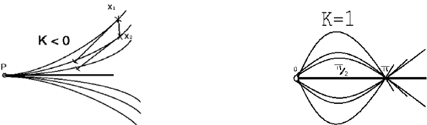
Figure 1: Left: Geodesic deviation on a manifold of negative curvature. (12) writes in polar coordinates $(\sigma,\theta)$: $\dot{\sigma}=-\frac{\sigma}{\lambda};\dot{\theta}=0$. The distance $\lVert\delta x\rVert$ between neighbors $x_{1}$ and $x_{2}$ decreases at a rate at least $\frac{1}{\lambda}$. Right: Geodesic deviation on the sphere.

Suppose that for all $t\in[0,T]$ $D(\hat{\xi},q(t))$ is bounded by the injectivity radius, as well as by $\frac{\pi}{4\sqrt{A}}$ in case of positive sectional curvature. At each time $t$ letting $P=q(t)$ we see that (7) is the same as (12). Lemma 1 thus proves that we have the property (13) at time $t$, with a contraction rate $\frac{2}{\lambda}$ independent from $t$. Thus Lemma 1 used at every $t$ proves that (7) is a contraction as defined in [12], [3]. Using the contraction interpretation in the appendix of [3] we see that if $\hat{\xi}_{1},\hat{\xi}_{2}$ are solutions of (7) we have

$$D(\hat{\xi}_{1}(t),\hat{\xi}_{2}(t))\leq e^{-\frac{1}{\lambda}t}D(\hat{\xi}_{1}(0),\hat{\xi}_{2}(0))\quad\forall t\in[0,T]$$

The system “forgets” its initial condition. So (9) holds if $\xi(t)$ is a solution of (7). This is true since $0={\frac{d}{dt}}D(\xi,q)=\lVert v\rVert_{g}-\lVert\dot{\xi}\rVert_{g}=\lVert v\rVert_{g}-\frac{1}{\lambda}D(\xi,q)$.

Under the basic assumption that $D(\hat{\xi},q(t))\leq I(t)$, we have just proved that when the sectional curvature is nonpositive in all planes, (9) is true for any initial condition. When the sectional curvature is bounded from above by $A$, we proved at Lemma 1 that (9) holds if for all $t>0$ $D(\hat{\xi},q(t))\leq\frac{\pi}{4\sqrt{A}}$, i.e. $\hat{\xi}$ remains in the contraction region. Thus, the bound on $\lambda$ is meant to make the contraction region a trapping region. Indeed ${\frac{d}{dt}}D(\hat{\xi},q)\leq\langle\text{grad}_{q}D(\xi,q),v\rangle-\lVert{\frac{d}{dt}}\hat{\xi}\rVert_{g}\leq\lVert v\rVert_{g}-\frac{1}{\lambda}D(\hat{\xi},q)$. Thus $D(\hat{\xi},q)=\frac{\pi}{4\sqrt{A}}$ implies ${\frac{d}{dt}}D(\hat{\xi},q)<0$ if ${\lambda}>\frac{\pi}{4\lVert v\rVert_{g}\sqrt{A}}$. Thus for ${\lambda}>\frac{\pi}{4\lVert v\rVert_{g}\sqrt{A}}$ the vector field is pointing inside the contraction region. In particular if $D(\hat{\xi}(0),q(0))<\frac{\pi}{4\sqrt{A}}$ we have $D(\hat{\xi}(t),q(t))<\frac{\pi}{4\sqrt{A}}$ for all $t>0$ and (9) holds.

Now that we have proved the exponential convergence of $D(\hat{\xi},\xi)$ we can focus on the convergence of $\hat{v}$ towards $\dot{q}$. $(q,\xi,\hat{\xi})$ is a geodetic triangle $T$. Indeed as $q,\xi,\hat{\xi}$ are assumed to be in a ball of radius $\frac{\pi}{4\sqrt{A}}$, $T$ is well-defined and the angles are less than $\pi$. The length of the sides are: $D(q,\xi)=\lambda\lVert\dot{q}\rVert$, which is fixed, $D(q,\hat{\xi})=\lambda\lVert\hat{v}\rVert$, and $D(\hat{\xi}(t),\xi(t))\leq\exp(-t/\lambda)D(\hat{\xi}(0),\xi(0))$. In the Euclidian case $(K\equiv 0)$, there is an homothety between $\hat{v},\dot{q}$ and the sides of the triangle and we have $\lambda\lVert\hat{v}-\dot{q}\rVert=D(\hat{\xi},\xi)$, proving (10). As $T$ and its sides belong to the surface $\Sigma$ defined before, one can apply Alexandrov’s theorem [19] stating that, if $A$ is an upper bound on the curvature, the angle $\alpha$ between $\dot{q}$ and $\hat{v}$ (the triangle angle at $q$) is less than the angle $\alpha_{A}$ corresponding to the case of constant curvature $K\equiv A$. Thus when the curvature is nonpositive in all planes, $\alpha$ is less than in the Euclidian case and (10) is proved. When the curvature is upper bounded by $A>0$, $\alpha$ is less that $\alpha_{A}$ verifying the spherical law of sines: $\sin(\alpha_{A})=\sin(\beta)\sin(\sqrt{A}~{}D(\hat{\xi},\xi))/\sin(\sqrt{A}~{}D(q,\xi))$, where $\beta$ is the opposite angle to the side linking $q$ and $\xi$ [19]. To prove (LABEL:speed:conv:eq2) we used $0\leq\sin\beta\leq 1$. The first part of (LABEL:speed:conv:eq2) is the spherical triangular inequality. $\alpha_{A}\rightarrow\pi$ is impossible as $D(\hat{\xi},\xi)\rightarrow 0$.

∎

3 Applications

3.1 Lagrangian mechanical system

Proposition 1.

Consider any Lagrangian system in a potential field in the admissible region defined by $U<E$. The observer

$$\frac{d}{dt}\hat{\xi}=-\frac{1}{\lambda}(E-U(q))~{}\overrightarrow{grad}_{\hat{\xi}}~{}D_{\hat{g}}^{2}(\hat{\xi},q)$$ (16)

is such that the Theorem 1 is valid in the Maupertuis time and Jacobi metric.

Proof.

One can apply the Maupertuis’ principle (see section 1.1). In Maupertuis’ time $\tau=\int_{0}^{t}2(E-U(q(t))dt$, the motion is a geodesic flow on the configuration space with modified metric $\hat{g}$, with $\lVert v\rVert_{\hat{g}}=1$ as $\hat{g}_{ij}(q)\frac{dq^{i}}{d\tau}\frac{dq^{j}}{d\tau}=2(E-U)g_{ij}(q)\frac{dq^{i}}{dt}\frac{dq^{j}}{dt}(\frac{dt}{d\tau})^{2}=1$. The observer defined by $\frac{d}{d\tau}\hat{\xi}=-\frac{1}{2\lambda}\overrightarrow{grad}_{\hat{\xi}}{D_{\hat{g}}}^{2}(\hat{\xi},q)$, $\lambda>0$ where $D_{\hat{g}}$ is the distance associated to Jacobi metric, is such that $\hat{v}=\mathcal{T}_{//\hat{\xi}\rightarrow q}\frac{d}{d\tau}\hat{\xi}$ is an estimation of $\frac{d}{d\tau}q$. ∎

For instance, R. Montgomery studied in a recent paper [16] the Newtonian equal-mass three bodies problem, with zero momentum and when the potential is taken equal to $1/r^{2}$: the Jacobi metric has negative curvature everywhere (except at two points). The reduced observer (16) is thus globally convergent for a three bodies system which is sensible to initial conditions.

Remark 1.

For a conservative system, the total energy $E$ needs to be known to compute the Jacobi metric. But no information about the direction of the velocity is required.

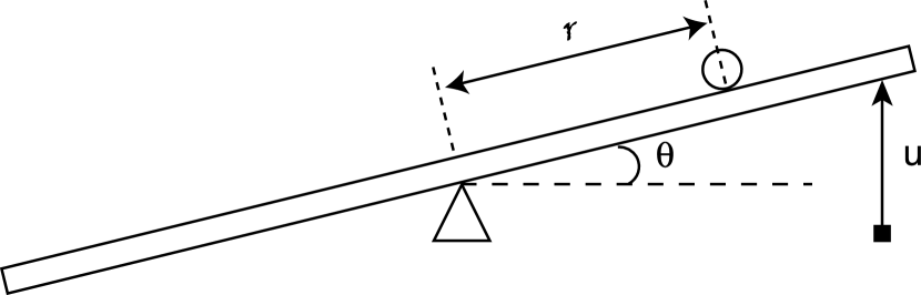
Figure 2: Ball and Beam

Remark 2.

Let us consider now a non-conservative system: the ball and beam of [3] with a torque control $u$ (see fig 2). The observer [3] is only locally convergent. Observer (7) can be used complementarily to provide a globally convergent estimator with the following little experiment. A some time $t_{0}$ maintain $u\equiv 0$ (no control) and set $\hat{\xi}(t_{0})=q(t_{0})$. The characteristic time of convergence of the observer (7) is $\tau=\lambda$ in the Maupertuis time. After a few $\tau$ the observer (7) provides the observer of Aghannan and Rouchon an initial estimation of the velocity close to the true one and from that moment $u$ can vary freely again: [3] converges. As the observer allows to identify the direction of the velocity, it is more interesting to use it for a 3D ball and beam problem in which the beam is replaced with a plate fixed at a point, rotating around two horizontal axis (so that two angles are involved).

3.2 Motion of a perfect incompressible fluid

The goal of this section is to show that the reduced observer could possibly be applied to more complicated systems. No formal proof is given but only heuristic discussions. The observer could be used in particle velocimetry as a (soft) velocimeter for a flow seeded with observable particles and modeled by Euler equations.

3.2.1 A reduced observer

Let us first introduce some results and notations of [5, 6, 18]. Let $\Omega$ be a domain of ${\mathbb{R}}^{3}$ bounded by a surface $\delta\Omega$. Let $\vec{v}$ be the velocity field of an ideal incompressible perfect fluid with density $\rho$ which fills the domain $\Omega$. The motion is described by the Euler equation

$${\frac{d}{dt}}{\vec{v}}+({\vec{v}}.\nabla){\vec{v}}=-\frac{1}{\rho}\nabla p$$ (17)

where $p$ is the pressure. Let SDiff $\Omega$ be the Lie group of all diffeomorphisms that preserve the Euclidian volume. Its Lie algebra ${\mathcal{U}}$ is the set or all vector fields of $\Omega$ of null divergence, and tangent to the boundary $\delta\Omega$. Consider the scalar product on the Lie algebra

$$\forall{\vec{v}},\vec{w}\in{\mathcal{U}},\quad<{\vec{v}},\vec{w}>={\rho}\int\int\int_{\Omega}{\vec{v}}(x).\vec{w}(x)dx$$ (18)

Let ${\vec{v}}(t)\in{\mathcal{U}}$ be a solution of (17). Let $\phi_{t}^{\vec{v}}(x)$ be the position at time $t$ of a fluid particle initially at $x$, i.e. obtained by integration on $[0,t]$ of the system $\frac{d}{ds}z={\vec{v}}(s,z),~{}z(0)=x$. $\phi_{t}^{\vec{v}}$ is a diffeomorphism for any $t>0$, and the motion of the fluid is described by a curve $t\mapsto\phi^{\vec{v}}_{t}$ on SDiff $\Omega$. Suppose $t$ is fixed. After a small time $\tau$ the diffeomorphism describing the fluid will be $\exp_{Id}(\tau{\vec{v}}(t))\phi_{t}^{\vec{v}}$ up to second order terms in $\tau$. It implies ${\vec{v}}(t)=DR_{(\phi_{t}^{\vec{v}})^{-1}}{\frac{d}{dt}}\phi_{t}^{\vec{v}}$ where $DR_{g}$ denotes the tangent map induced by right multiplication by $g$ on the group. Thus the kinetic energy of the fluid $T=\frac{1}{2}\langle{\vec{v}},{\vec{v}}\rangle$ defines a right-invariant metric. The least action principle implies that the fluid motion $t\mapsto\phi^{\vec{v}}_{t}$ is a geodesic flow on SDiff $\Omega$ endowed with the kinetic energy metric. Thus ${\nabla}^{LC}_{\vec{v}}{\vec{v}}=0$ where the Levi-Civita covariant differentiation ${\nabla}^{LC}$ is given by $\huge{\nabla}^{LC}_{\vec{v}}\vec{\eta}=\frac{\partial}{\partial t}\xi+({\vec{v}}\cdot\nabla)~{}\vec{\eta}+\nabla{\alpha}$ and $\alpha$ is a real function such that ${\nabla}^{LC}_{\vec{v}}~{}\vec{\eta}\in{\mathcal{U}}$. For fixed $t$, the virtual displacement corresponding to $\delta x$ in lemma 1 can be defined and identified to an element of ${\mathcal{U}}$. It satisfies a Jacobi equation along the geodesic (see Proposition 2 of [18]).

The reduced observer is defined intrinsically and can formally be applied to this fluid velocity estimation problem. The Theorem 1 is valid, as the proof is only made of intrinsic calculations, and its core is the Jacobi equation which gives conditions under which $\sigma\frac{\partial}{\partial\sigma}G\geq G$. The observer’s state $\hat{\xi}$ is a virtual fluid, defined as a solution of (7), where $q$ is replaced by $\phi_{t}^{\vec{v}}$. Using the right group multiplication one can define $\zeta(t)=\hat{\xi}(t)\circ(\phi_{t}^{\vec{v}})^{-1}$. Note that $\zeta$ must remain in the group identity connected component so that (7) is well-defined.

3.2.2 Discussion on the convergence and curvature

When the curvature is bounded from above by $A=-B^{2}<0$, the geodesic flow is sensitive to initial conditions, and admits ergodic properties [5]. Surprisingly, in this case the observer is globally exponentially convergent by Theorem 1. When there are always sections with negative curvature along a geodesic, it is commonly assumed that the sensitivity to initial conditions is still valid.

We have the following formal convergence result: consider a sinusoidal parallel stationary motion of a fluid in the tore $T^{2}=\{(x,y),~{}x\mod 2\pi,~{}y\mod 2\pi\}$ given by the current function $\psi=\cos(kx+ly)$ with $k,l\in\mathbb{N}$, and the velocity vector field $\vec{v}=\text{rot}~{}\psi$. Take $\hat{\xi}(0)={\phi^{\vec{v}}_{0}}$ for (7). Then $\lVert\hat{v}(t)-\vec{v}\rVert$ converges exponentially to $0$. The proof is obvious as both points belong to the same geodesic. But one can expect a great robustness to measurement noise. Indeed [5] proves the motion defined by $\psi$ is a geodesic of SDiff $T^{2}$, and the curvature is non positive in all planes containing $\vec{v}(x,y)$. Moreover it is zero only in a family of planes of null measure. But by Theorem 1 negative curvature implies global stability, and small positive curvature implies a large basin of attraction.

More generally, Arnol’d [5] considers the group S₀Diff $T^{2}$ of diffeomorphisms preserving the center of gravity. Calculations show the curvature is positive “only in a few sections”. He suggests to consider the mean curvature along paths to characterize the stability of the flow. As a consequence, if the atmosphere was a bidimensional incompressible fluid on the earth viewed as $T^{2}$ (identify opposite sides of the planisphere), the wind should be known up to 5 decimals for a two-months weather’s prediction. Following this suggestion, as the curvature is positive in only in a few sections, one could expect a good global behavior of the observer.

4 Simulations on the sphere

Consider the inertial motion of a material point constrained to lie on the sphere ${\mathbb{S}}^{2}$. The speed is constant (see section 1.2) and assumed to be equal to $1$. One can always choose coordinates $q=(q_{x},q_{y},q_{z})\in{\mathbb{R}}^{3}$ such that the motion writes: $\dot{q}_{x}(t)=\cos(t),~{}\dot{q}_{y}(t)=\sin(t),~{}\dot{q}_{z}(t)=0$. Let $\hat{\xi}=(\hat{\xi}_{x},\hat{\xi}_{y},\hat{\xi}_{z})\in{\mathbb{R}}^{3}$. The observer equation (7) writes

$${\frac{d}{dt}}{\hat{\xi}_{x}} =\frac{1}{\lambda}\varphi~{}\frac{((q\wedge\hat{\xi})\wedge\hat{\xi})_{x}}{\parallel(q\wedge\hat{\xi})\wedge\hat{\xi}\parallel},\quad{\frac{d}{dt}}{\hat{\xi}_{y}}=\frac{1}{\lambda}\varphi~{}\frac{((q\wedge\hat{\xi})\wedge\hat{\xi})_{y}}{\parallel(q\wedge\hat{\xi})\wedge\hat{\xi}\parallel},$$

$${\frac{d}{dt}}{\hat{\xi}_{z}} =\frac{1}{\lambda}\varphi~{}\frac{((q\wedge\hat{\xi})\wedge\hat{\xi})_{z}}{\parallel(q\wedge\hat{\xi})\wedge\hat{\xi}\parallel}$$

where $\lambda<0$ and $\varphi$ is the angle between $q$ and $\hat{\xi}$. As the geodesics of the sphere are great circles, $\varphi$ is the geodesic length between those two points. The inital conditions are : $q(0)=[1,0,0]^{T}$ and $\hat{\xi}(0)=\frac{1}{\sqrt{2}}[0,1,1]^{T}$. To simulate the sensor’s imperfections a white noise whose amplitude is 20$\%$ of the maximal value of the signal was added. $\hat{\xi}$ converges to the equator, and asymptotically follows $q$ at a distance $\lvert\lambda\rvert$. The parallel transport $\hat{v}$ of ${\frac{d}{dt}}\hat{\xi}$ is an estimation of $v$ (not noisier than the measured signal). In fact for $\lambda<\pi/2$ the observer always converges in simulation, and for $\lambda>\pi/2$ it does not.

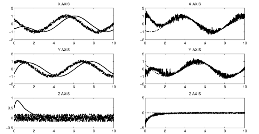
Figure 3: Simulations on the sphere for $\lambda=\pi/4$. Left: Measured $q$ (dashed line) and $\hat{\xi}$ (plain line). Right: velocity $v$ (dashed) and estimation $\hat{v}$ (plain).

5 Conclusion

We designed a nonlinear globally convergent reduced observer for conservative Lagrangian systems. The observer is intrinsic and converges despite the effects of curvature: instability of the flow and gyroscopic terms. The tuning of the gains is simple. The only gain is a scalar which must be set in function of the noise and the maximal curvature. The observer can be used for velocity estimation for all systems described by geodesic flows ($\nabla_{v}v=0$), notably conservative Lagrangian system, and the motion of an incompressible fluid. Using the Maupertuis principle this work could be extended to the case of a mixture of compressible fluids [17].

Unfortunately when the motion is described by $\nabla_{v}v=S(q)$ with $S$ known (Lagrangian system with external forces) the reduced observer does not converge. Including such terms $S$ remains an open question. As a concluding remark, note that the article gives insight in the link between convergence and geometrical structure of the model in the theory of observers, complementing the work of [3, 15] and more recent results [8].

6 Acknowledgements

I am indebted to Ivan Kupka and Pierre Rouchon for very useful discussions.

References

- [1] R. Abraham and J.E. Marsden. Foundations of Mechanics. Addison-Wesley (updated 1985 printing), second edition, 1985.
- [2] N. Aghannan and P. Rouchon. On invariant asymptotic observers. In 41st IEEE Conference on Decision and Control, pages 1479–1484, 2002.
- [3] N. Aghannan and P. Rouchon. An intrinsic observer for a class of lagrangian systems. IEEE AC, 48(6):936–945, 2003.
- [4] V. Arnold. Ordinary Differential Equations. Mir Moscou, 1974.
- [5] V. Arnold. Mathematical Methods of Classical Mechanics. Mir Moscou, 1976.
- [6] V.I. Arnol’d. Sur la géométrie différentielle des groupes de lie de dimension infinie et ses applications à l’hydrodynamique des fluides parfaits. Ann. Inst. Fourier, 16:319–361, 1966.
- [7] S. Bonnabel, Ph. Martin, and P. Rouchon. Symmetry-preserving observers. IEEE Trans. on Automatic Control, 53(11):2514–2526, 2008.
- [8] S. Bonnabel, Ph. Martin, and P. Rouchon. Non-linear symmetry-preserving observers on lie groups. IEEE Trans. on Automatic Control, 54(7):1709 – 1713, 2009.
- [9] S. Bonnabel, M. Mirrahimi, and P. Rouchon. Observer-based hamiltonian identification for quantum systems. Automatica, 45(11):1144–1155, 2009.
- [10] F. Bullo, N.E. Leonard, and A.D. Lewis. Controllability and motion algorithms for underactuated lagrangian systems on lie groups. IEEE Trans. Automat. Control, 35:1437–1454, 2000.
- [11] A.D. Lewis and R.M. Murray. Configuration controllability of simple mechanical control systems. SIAM Journal on Control and Optimization, 35:766–790, 1997.
- [12] W. Lohmiler and J.J.E. Slotine. On metric analysis and observers for nonlinear systems. Automatica, 34(6):683–696, 1998.
- [13] D. Luenberger. An introduction to observers. IEEE Trans. on Automatic Control, 16(6):596–602, 1971.
- [14] R. Mahony, T. Hamel, and J-M Pflimlin. Nonlinear complementary filters on the special orthogonal group. IEEE-Trans. on Automatic Control, 53(5):1203–1218, 2008.
- [15] D. H. S. Maithripala, W. P. Dayawansa, and J. M. Berg. Intrinsic observer-based stabilization for simple mechanical systems on lie groups. SIAM J. Control and Optim., 44:1691–1711, 2005.
- [16] R. Montgomery. Hyperbolic pants fit a three-body problem. Ergod. Thy. Dyn. Sys., 25:921–947, 2005.
- [17] P. Rouchon. Dynamique des fluides parfaits, principe de moindre action, stabilité lagrangienne. Technical Report 13/3446 EN, ONERA, september 1991.
- [18] P. Rouchon. On the Arnol’d stability criterion for steady-state flows of an ideal fluid. European Journal of Mechanics /B Fluids, 10:651–661, 1991.
- [19] J.J. Stoker. Differential Geometry. Wiley-Interscience, 1969.