Stochastic Modeling of Unresolved Scales
in Complex Systems

Abstract

Model uncertainties or simulation uncertainties occur in mathematical modeling of multiscale complex systems, since some mechanisms or scales are not represented (i.e., “unresolved”) due to lack in our understanding of these mechanisms or limitations in computational power. The impact of these unresolved scales on the resolved scales needs to be parameterized or taken into account. A stochastic scheme is devised to take the effects of unresolved scales into account, in the context of solving nonlinear partial differential equations. An example is presented to demonstrate this strategy.

Key Words: Stochastic partial differential equations (SPDEs); stochastic modeling; impact of unresolved scales on resolved scales; model error; large eddy simulation (LES); fractional Brownian motion

Mathematics Subject Classifications (2000): 60H30, 60H35, 65C30, 65N35

1 Introduction

Mathematical models for scientific and engineering systems often involve with some uncertainties. We may roughly classify such uncertainties into two kinds. The first kind of uncertainties may be called model uncertainty. They involve with physical processes that are less known, not yet well understood, not well-observed or measured, and thus difficult to be represented in the mathematical models.

The second kind of uncertainties may be called simulation uncertainty. This arises in numerical simulations of multiscale systems that display a wide range of spatial and temporal scales, with no clear scale separation. Due to the limitations of computer power, at present and for the conceivable future, not all scales of variability can be explicitly simulated or resolved. Although these unresolved scales may be very small or very fast, their long time impact on the resolved simulation may be delicate (i.e., may be negligible or may have significant effects, or in other words, uncertain). Thus, to take the effects of unresolved scales on the resolved scales into account, representations or parameterizations of these effects are desirable.

These uncertainties are sometimes also called unresolved scales, as they are not represented or not resolved in modeling or simulation. Model uncertainties have been considered in, for example, [10, 13, 12, 2, 39, 17, 26, 27, 28] and references therein. Works relevant for parameterizing unresolved scales include [15, 14, 18, 34, 3, 7, 40, 41, 33, 4], among others.

In this paper we consider an issue of approximating model uncertainty or simulation uncertainty (unresolved scales) by stochastic processes, and then devise a stochastic scheme for such approximations. We first recall some basic facts about fractional Brownian motion (fBM) in §2. Then we discuss model uncertainty and simulation uncertainty in §3 and §4, respectively. Finally, we present an example in §5 demonstrating our result. This example involves approximating subgrid scales via correlated noises, in the context of large eddy simulations of a partial differential equation.

2 Fractional Brownian motion and colored noise

We discuss a model of colored noise in terms of fractional Brownian motion (fBM), including a special case which is white noise in terms of usual Brownian motion. The fractional Brownian motion $B^{H}(t)$, indexed by a so called Hurst parameter $H\in(0,1)$, is a generalization of the more well-known process of the usual Brownian motion $B(t)$. It is a centered Gaussian process with stationary increments. However, the increments of the fractional Brownian motion are not independent, except in the usual Brownian motion case ($H=\frac{1}{2}$). For more details, see [25, 23, 8, 20, 38].

Definition of fractional Brownian motion: For $H\in(0,1)$, a Gaussian process $B^{H}(t)$, or $fBM(t)$, is a fractional Brownian motion if it starts at zero $B^{H}(0)=0,\;a.s.$, has mean zero ${\mathbb{E}}[B^{H}(t)]=0$, and has covariance ${\mathbb{E}}[B^{H}(t)B^{H}(s)]=\frac{1}{2}(|t|^{2H}+|s|^{2H}-|t-s|^{2H})$ for all t and s. The standard Brownian motion is a fractional Brownian motion with Hurst parameter $H=\frac{1}{2}$.

Some properties of fractional Brownian motion: A fractional Brownian motion $B^{H}(t)$ has the following properties:
(i) It has stationary increments;
(ii) When $H=1/2$, it has independent increments;
(iii) When $H\neq 1/2$, it is neither Markovian, nor a semimartingale.

We use the Weierstrass-Mandelbrot function to approximate the fractional Brownian motion. The basic idea is to simulate fractional Brownian motion by randomizing a representation due to Weierstrass. Given the Hurst parameter $H$ with $0<H<1$, we define the function $w(t)$ to approximate the fractional Brownian motion:

$$w(t_{i})=\sum^{\infty}_{j=-\infty}C_{j}r^{jH}\sin(2\pi r^{-j}t_{i}+d_{j})$$

where $r=0.9$ is a constant, $C_{j}$’s are normally distributed random variables with mean $0$ and standard deviation $1$, and the $d_{j}$’s are uniformly distributed random variables in the interval $0\leq d_{j}<2\pi$. The underlying theoretical foundation for this approximation can be found in [31, 22]. Figures 1 and 2 show a sample path of the usual Brownian motion (i.e., $H=\frac{1}{2}$), and fractional Brownian motion with Hurst parameter $H=\frac{3}{4}$, respectively.

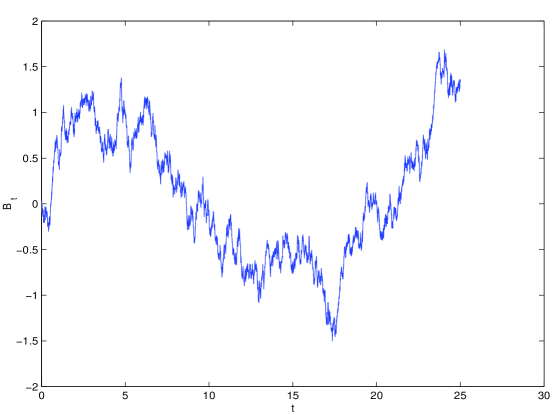
Figure 1: A sample path of Brownian motion $B(t)$

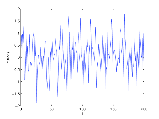
Figure 2: A sample path of fractional Brownian motion $B^{H}(t)$, with $H=0.75$

3 Model uncertainty

We consider a spatially extended system modeled by a partial differential equation (PDE):

$$u_{t}=Au+N(u),$$ (1)

where $A$ is a linear (unbounded) differential operator, and $N$ is a nonlinear function of $u(x,t)$ with $x\in D$ and $t>0$, and satisfies a local Lipschitz condition. In fact, $N$ may also depend on the gradient of $u$.

If this (deterministic) model is accurate, i.e., its prediction on the field $u$ matches with the observational data $\tilde{u}$ on a certain period of time $[0,T]$, then there is no need for a stochastic approach. However, when the prediction $u$ deviates from the observational data $\tilde{u}$, we then need to modify the model (1). In this case, the observational data $\tilde{u}$ may be thought to satisfy a modified model:

$$\tilde{u}_{t}=A\tilde{u}+N(\tilde{u})+F(\tilde{u}),$$ (2)

where the model uncertainty $F(\tilde{u})$ is usually a fluctuating (i.e., random) process, as the observational data $\tilde{u}$ is so (i.e., has various samples or realizations).

The model discrepancy or model uncertainty $F(\tilde{u})$ may have various causes, such as missing physical mechanisms (not represented in the deterministic model (1)). Sometimes, the model uncertainty $F(\tilde{u})$ is smaller in magnitude than other terms in the model (2) and thus is often ignored in the deterministic modeling. However, being small and being fluctuating may not necessarily imply that its impact on the overall system evolution to be small [1]. To take this impact into account, we would like to model or approximate $F(\tilde{u})$ by a stochastic process.

We first calculate the model uncertainty $F(\tilde{u})$ via observational data $\tilde{u}$. By discretizing (2) and using data samples for $\tilde{u}$, we obtain (discretized) samples for $F$.

The time correlation may then be calculated using the samples of $F$. If the time correlation scale is significantly shorter than the time scale for the field $u$, we may ignore the time correlation and thus approximate $F$ by the following stochastic process containing a (uncorrelated) white noise, for example:

$$F=f+\sigma\;\tilde{u}\dot{B}_{t},$$ (3)

where $f={\mathbb{E}}F$ is the mean of $F$ (computed from data), $B_{t}$ is the usual Brownian motion (reviewed in §5 below) and the deterministic noise intensity $\sigma$ may depend on space. Here $\sigma$ may be computed via stochastic calculus, especially the Ito isometry, as follows.

$$F-{\mathbb{E}}F = \sigma\;\tilde{u}\dot{B}_{t},$$

$${\mathbb{E}}[\int_{0}^{T}(F-{\mathbb{E}}F)dt]^{2} = \sigma^{2}\;{\mathbb{E}}[\int_{0}^{T}\tilde{u}dB_{t}]^{2},$$

$${\mathbb{E}}[\int_{0}^{T}(F-{\mathbb{E}}F)dt]^{2} = \sigma^{2}\;{\mathbb{E}}\int_{0}^{T}\tilde{u}^{2}(x,t)dt,$$

Thus we obtain

$$\sigma=\sqrt{\frac{{\mathbb{E}}[\int_{0}^{T}(F-{\mathbb{E}}F)dt]^{2}}{{\mathbb{E}}\int_{0}^{T}\tilde{u}^{2}(x,t)dt}}\;.$$ (4)

With this approximation, we obtain the following stochastic partial differential equation (SPDE) as a modified model for the original deterministic model (1): $U\approx\tilde{u}$

$$U_{t}=AU+N(U)+f(U)+\sigma\;\tilde{u}\dot{B}_{t}.$$ (5)

In general, the model uncertainty $F$ may be better approximated by correlated noise via fractional Brownian motion. Since the procedure is similar, we will demonstrate this in the next section when we discuss simulation uncertainty.

4 Simulation uncertainty

This section deals with simulation uncertainty, i.e., stochastically parameterizing the effects of the unresolved scales on the resolved scales. We consider this issue in the context of large eddy simulations (LES) of a nonlinear partial differential equation with memory.

In large eddy simulations of fluid or geophysical fluid flows [33, 4], the unresolved scales appear as the so-called subgrid scales (SGS). The SGS term appears to be highly fluctuating (“random”); see the Figure 1 in [24]. Partially motivated by this, stochastic parameterizations of subgrid scales have been investigated in fluid, geophysical and climate simulations, based on physical or intuitive or empirical arguments. Another, perhaps more important, motivation for applying stochastic parameterizations of subgrid scales is to induce the desired backward energy flux (“stochastic backscatter”) in fluid simulations [16, 21, 35].

We present one stochastic parameterization scheme of the subgrid scale term in the large eddy simulation of a nonlinear partial differential equation with an extra memory term, which is in fact a nonlinear integro-partial differential equation. The approximation scheme is based on stochastic calculus involving with a fractional Brownian Motion, and the “parameter’ to be calculated is a spatial function, which is derived using Ito stochastic calculus.

$$u_{t}=Au+F(u),$$ (6)

where $A$ is a linear differential operator, and $F$ is a nonlinear function of $u(x,t)$ with $x\in D$and $t>0$, and satisfies a local Lipschitz condition. We investigate stochastic parameterizations of unresolved scales in the context of large eddy simulations of the above system.

The idea of large eddy simulation is to split the flow into a local, spatial mean (or average) and a fluctuation about the that mean. The mean $\bar{u}$ is defined by filtering or mollification (convolution with an approximate identity). The goal is to predict the mean accurately. This is widely believed possible based on the idea that since fluctuations have random character, their average effects on the mean notion can successfully be medelled.

To filter the solution, we pick a filter. Many different ones are commonly used. To fix the ideas, in this paper, we use Gaussian filter as in [4], $G_{\delta}(x)=\frac{1}{\pi\delta^{2}}e^{-\frac{x^{2}}{\delta^{2}}},$ where $\delta>0$ is the filter size and the filter is such that: (i) $u*G_{\delta}$ is infinitely differentiable in space and, (ii) $u*G_{\delta}\to u$ as $\delta\to 0$ in $L^{2}(D)$. Here and hereafter $u*G_{\delta}=\int_{D}u(y,t)G_{\delta}(x-y)dy$ or the over bar $\bar{u}$ denotes convolution.

Remark 1.

The mean $\bar{u}$ is a weighted average of $u$ about the point $x$. As $\delta\to 0$, the points near $x$ are weighted more and more heavily, so $u*G_{\delta}\to u$ as $\delta\to 0$ in $L^{2}(D)$.

Using the fact that convolution commutes with differentiatian, we get the space-filtered system:

$$\bar{u}_{t}=A\bar{u}+\overline{F(u)},$$

or

$$\bar{u}_{t}=A\bar{u}+F(\bar{u})+R(u,\bar{u}),$$ (7)

where the subgrid scale term $R(u,\bar{u}):=\overline{F(u)}-F(\bar{u})$. Since generally $\overline{F(u)}\neq F(\bar{u})$, the usual parameterization or closure problem of the large eddy simulation has arisen. Due to inaccurate (uncertain) initial conditions or boundary conditions, $R(u,\bar{u})$ is a correlated fluctuating process [24, 7], depending on samples $\omega$ in a suitable sample space $\Omega$. We thus would like to approximate the subgrid scale term $R(u,\bar{u})$ by a stochastic process with a correlated (i.e., colored) noise component, for example:

$$R=f(\bar{u})+\sigma(x)\frac{dB^{H}_{t}}{dt},$$ (8)

where $\frac{dB^{H}_{t}}{dt}$ is a colored noise (generalized time derivative of a fractional Brownian motion; reviewed in §5 below), and

$$f(\bar{u})={\mathbb{E}}R,$$ (9)

is the mean component of the subgrid scale term $R$. Moreover, the noise intensity $\sigma(x)$ is a non-negative deterministic function to be determined from fluctuating SGS data $R$. The subgrid scale term $R$ may be inferred from observational data (see [29, 30] for relevant information for subgrid scales in Navier-Stokes equations), or from fine mesh simulations.

Note that $\sigma$ is to be calculated or estimated from the fluctuating SGS data $R$, either from observation or from fine mesh simulations. So this is an inverse problem. As in usual inverse problems [36], the stochastic parameterizations for the SGS term $R$ is not unique. What we proposed above is merely an example. This offers an opportunity for trying various stochastic parameterization schemes, much as one uses various smoother functions (e.g., polynomials or Fourier series) to approximate less regular functions or data in deterministic approximation theory.

To estimate the unknown parameter (function) $\sigma(x)$, we start with the following relation:

$$R-{\mathbb{E}}R = \sigma(x)\frac{dB^{H}_{t}}{dt}.$$ (10)

Taking time integral over a computational interval $[0,T]$ on both sides, we obtain

$$\int_{0}^{T}[R-{\mathbb{E}}R]dt=\int_{0}^{T}\sigma(x)d{B}^{H}_{t}=\sigma(x)B^{H}_{T}.$$

Therefore, taking mean-square on both sides,

$${\mathbb{E}}(\int_{0}^{T}[R-{\mathbb{E}}R]dt)^{2} = \sigma^{2}(x)T^{2H}.$$

Thus an estimator for $\sigma(x)$ is

$$\sigma(x)=\frac{1}{T^{H}}\sqrt{{\mathbb{E}}(\int_{0}^{T}[R-{\mathbb{E}}R]dt)^{2}}\;\;,$$ (11)

which can be computed numerically.

By the stochastic parameterization (8) on the SGS term $R$, with $f$ determined from (9) and $\sigma$ from (11), the LES model (7) becomes a stochastic partial differential equation (SPDE) for the large eddy solution $U\approx\bar{u}$:

$$U_{t}=AU+N(U)+f(U)+\sigma(x)\frac{dB^{H}_{t}}{dt},$$ (12)

with the appropriately filtered boundary condition and filtered initial condition.

5 An example

We present a specific example of stochastic modeling of simulation uncertainty of subgrid scales, in the context of large eddy simulations. We consider the following nonlinear partial differential equation with a memory term (time-integral term) [6]:

$$u_{t} = u_{xx}+u-u^{3}+\int^{t}_{0}{1\over{1+|t-s|^{\beta}}}\;u(x,s)ds,$$ (13)

under appropriate initial condition $u(x,0)=u_{0}(x)$ and boundary conditions $u(-1,t)=a,\;u(1,t)=b$ with $a,b$ constants, on a bounded domain $D:-1\leq x\leq 1$. Here $\beta$ is a positive constant. This model arises in mathematical modeling in ecology [42], heat conduction in certain materials [11, 19] and materials science [9, 19]. The time-integral term here represents a memory effect depending on the past history of the system state, and this memory effect decays polynomially fast in time.

The large eddy solution $\bar{u}$ is the true solution $u$ looked through a filter: i.e., through convolution with a spatial filter $G_{\delta}(x)$, with spatial scale (or filter size or cut-off size) $\delta>0$:

$$\bar{u}(x,t):=u*G_{\delta}=\int_{D}u(y,t)G_{\delta}(x-y)dy.$$

In this paper, we use a Gaussian filter as in [4], $G_{\delta}(x)=\frac{1}{\pi\delta^{2}}e^{-\frac{x^{2}}{\delta^{2}}}$.

On convolving (13) with $G_{\delta}$, the large eddy solution $\bar{u}$ is to satisfy

$$\bar{u}_{t} = \bar{u}_{xx}+\bar{u}-\overline{u^{3}}+\int^{t}_{0}{1\over{1+|t-s|^{\beta}}}\bar{u}(x,s)ds,$$

or

$$\bar{u}_{t} = \bar{u}_{xx}+\bar{u}-{\bar{u}}^{3}+\int^{t}_{0}{1\over{1+|t-s|^{\beta}}}\;\bar{u}(x,s)ds+R(x,t),$$ (14)

where the remainder term, i.e., the subgrid scale (SGS) term $R(x,t)$ is defined as

$$R(x,t):=({\bar{u}})^{3}-\overline{(u^{3})}.$$ (15)

We can write $u=\bar{u}+u^{\prime}$ with $\bar{u}$ the large eddy term and $u^{\prime}$ the fluctuating term. Note that $\bar{u}=u-u^{\prime}$. So the SGS term $R(x,t)$ involves nonlinear interactions of fluctuations $u^{\prime}$ and the large eddy flows. Thus $R(x,t)$ may be regarded as a function of $\bar{u}$ and $u^{\prime}$: $R:=R(\bar{u},u^{\prime})$.

The leads to a possibility of approximating $R(x,t)$ by a suitable stochastic process defined on a probability space $(\Omega,\mathcal{F},\mathbb{P})$, with $\omega\in\Omega$, the sample space, $\sigma-$field $\mathcal{F}$ and probability measure $\mathbb{P}$. This means that we treat $R$ data as random data as in [24], which take different realizations, e.g., due to fluctuating observations or due to numerical simulation with initial and boundary conditions with small fluctuations. In fluid or geophysical fluid simulations, the SGS term may be highly fluctuating and time-correlated [24], and this term may be inferred from observational data [29, 30], or from fine mesh simulations.

This further suggests for parameterizing the subgrid scale term $R(x,t)$ as a time-correlated or colored noisy term. The increments of fractional Brownian motion are correlated in time and hence its generalized time derivative $\dot{B}_{t}^{H}$ is used as a model for colored noise. In the special case $H=\frac{1}{2}$, we have the white noise $\dot{B}_{t}$. Thus we parameterize the subgrid scale term $R(x,t)$, which is time-correlated, by colored noise $\dot{B}_{t}^{H}$ as follows:

$$R(x,t)=f(\bar{u})+\sigma(x)\frac{dB^{H}_{t}}{dt},$$ (16)

where

$$f(\bar{u})={\mathbb{E}}R(x,t),$$ (17)

is the mean component of the subgrid scale term $R(x,t)$. Moreover, the noise intensity $\sigma(x)$ is a non-negative deterministic function to be determined from fluctuating SGS data $R$. The subgrid scale term $R(x,t)$ may be inferred from observational data [29, 30], or from fine mesh simulations as we do here. We represent the mean component $f(\bar{u})$ in terms of the large eddy solution $\bar{u}$. The specific form for $f$ depends on the nature of the mean of $R$. Here we take $f(\bar{u})=a_{0}+a_{1}u+a_{2}u^{2}+a_{3}u^{3}$, where coefficients $a_{i}$’s are determined via data fitting by minimizing $\int_{0}^{T}\int_{D}[a_{0}+a_{1}u+a_{2}u^{2}+a_{3}u^{3}-{\mathbb{E}}R(x,t)]^{2}dxdt$. Moreover, we take $B_{t}^{H}$ as a scalar fractional Brownian motion.

Note that $\sigma$ is to be calculated or estimated from the fluctuating SGS data $R$, either from observation or (in this paper) from fine mesh simulations; see detailed discussions in [24, 7]. So this is an inverse problem. As in usual inverse problems [36], the stochastic parameterizations for the SGS term $R$ is not unique. This offers an opportunity for trying various stochastic parameterization schemes, much as one uses various smoother functions (e.g., polynomials or Fourier series) to approximate less regular functions or data in deterministic approximation theory.

To estimate the unknown parameter (function) $\sigma(x)$, we start with (16)-(17) to get the following relation:

$$R(x,t)-{\mathbb{E}}R(x,t) = \sigma(x)\frac{dB^{H}_{t}}{dt}.$$ (18)

Taking time integral over a computational interval $[0,T]$ on both sides, we obtain

$$\int_{0}^{T}[R(x,t)-{\mathbb{E}}R(x,t)]dt=\int_{0}^{T}\sigma(x)d{B}^{H}_{t}=\sigma(x)B^{H}_{T}.$$

Therefore, taking mean-square on both sides,

$${\mathbb{E}}(\int_{0}^{T}[R(x,t)-{\mathbb{E}}R(x,t)]dt)^{2} = \sigma^{2}(x)T^{2H}.$$

Thus an estimator for $\sigma(x)$ is

$$\sigma(x)=\frac{1}{T^{H}}\sqrt{{\mathbb{E}}(\int_{0}^{T}[R(x,t)-{\mathbb{E}}R(x,t)]dt)^{2}}\;\;,$$ (19)

which can be computed numerically.

By the stochastic parameterization (16) on the SGS term $R$, with $f$ determined from (17) and $\sigma$ from (19), the LES model (14) becomes a stochastic partial differential equation (SPDE) for the large eddy solution $U\approx\bar{u}$:

$$U_{t}=U_{xx}+U-U^{3}+\int^{t}_{0}{1\over{1+|t-s|^{\beta}}}\;U(x,s)ds+f(U)+\sigma(x)\frac{dB^{H}_{t}}{dt},$$ (20)

with boundary conditions $U(-1,t)=a,\;U(1,t)=b$ and filtered initial condition

$$U(x,0)=\bar{u}_{0}(x).$$ (21)

Numerical Experiments:

We use a spectral method to solve nonlinear system (13) and (20) numerically. For more details, please see [37]. We take the following initial and boundary conditions:

$$u(x,0)=u_{0}=0.53x-0.47sin(1.5\pi x),\;\;u(-1,t)=-1,\;\;u(1,t)=1$$

Fine mesh simulations of the original system with memory (13) are conducted to generate benchmark solutions or solution realizations, with initial conditions slightly perturbed; see Fig. 3. These fine mesh solutions $u$ are used to generate the SGS term $R$ defined in (15) at each time and space step. The filter size used in calculating $R$ is taken as $\delta=0.01$. The mean $f$ is calculated from (17) via cubic polynomial data fitting (as discussed in the last section), and parameter function $\sigma(x)$ is calculated as in (19). The stochastic LES model (20) is solved by the same numerical code but on a coarser mesh. Note that a four times coarser mesh simulation with no stochastic parameterization for the original system (13) does not generate satisfactory results; see Fig. 4. The stochastic LES model (20) is then solved in the mesh four times coarser than the fine mesh used to solve the original equation (13). The stochastic parameterization leads to better resolution of the solution as shown in Fig. 5. As in [7], it can be shown that when two stochastic parameterization terms are close in mean-square norm on finite time intervals, the solutions are also close in the same norm.

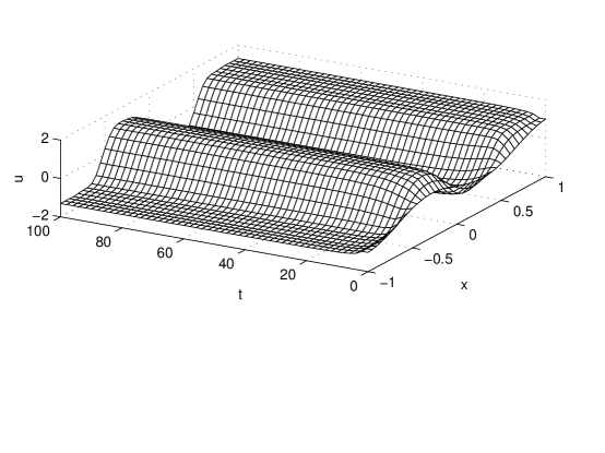
Figure 3: Solution to the original system on a fine mesh, $u_{t}=u_{xx}+u-u^{3}+\int^{t}_{0}{1\over{1+|t-s|^{\beta}}}\;u(x,s)ds$, $\beta=2$, mesh size $\Delta x=0.001$.

Figure 4: Solution to the original system with NO stochastic parametrization on the mesh four times coarser than the mesh used in Fig. 3, $u_{t}=u_{xx}+u-u^{3}+\int^{t}_{0}{1\over{1+|t-s|^{\beta}}}\;u(x,s)ds$, $\beta=2$.

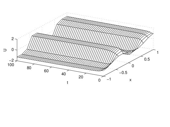
Figure 5: Solution to LES model with stochastic parametrization on the mesh four times coarser than the mesh used in Fig. 3, $U_{t}=U_{xx}+U-U^{3}+\int^{t}_{0}{1\over{1+|t-s|^{\beta}}}\;U(x,s)ds+f(U)+a(x)\dot{B}^{H}_{t}$, $\beta=2$, $H=\frac{3}{4}$.

References

- [1] L. Arnold, Random Dynamical Systems. Springer-Verlag, New York, 1998.
- [2] L. Arnold, Hasselmann’s program visited: The analysis of stochasticity in deterministic climate models. In J.-S. von Storch and P. Imkeller, editors, Stochastic climate models. pages 141–158, Boston, 2001. Birkhäuser.
- [3] P. S. Berloff, Random-forcing model of the mesoscale oceanic eddies. J. Fluid Mech. 529 (2005), 71-95.
- [4] L.C. Berselli, T. Iliescu and W. J. Layton. Mathematics of Large Eddy Simulation of Turbulent Flows. Springer Verlag, 2005.
- [5] P. F. Craigmile, Simulating a class of stationary Gaussian processes using the Davies-Harte algorithm, with application to long memory processes. J. Time Series Anal. 24 (2003), 505-511.
- [6] A. Du and J. Duan, A stochastic approach for parameterizing unresolved scales in a system with memory. Submitted, 2007.
- [7] J. Duan and B. Nadiga, Stochastic parameterization of large eddy simulation of geophysical flows. Proc. American Math. Soc. 135 (2007), 1187-1196.
- [8] T. E. Duncan, Y. Z. Hu, B. Pasik-Duncan, Stochastic Calculus for Fractional Brownian Motion. I: Theory. SIAM Journal on Control and Optimization 38 (2000), 582-612.
- [9] G.A. Francfort and P.M. Suquet, Homognization and mechanical dissipation in thermo-viscoelasticity, Arch. Ratinal Mech. Anal., 96(1986) 879-895.
- [10] J. Garcia-Ojalvo and J. M. Sancho, Noise in Spatially Extended Systems. Springer-Verlag, 1999.
- [11] C. Giorgi, A. Marzocchi and V. Pata, Asymptotic behavior of a similinear problem in heat conduction with memory, NoDEA Nonl. Diff. Equa. Appl., 5(1998) 333-354.
- [12] K. Hasselmann, Stochastic climate models: Part I. Theory. Tellus, 28 (1976), 473-485.
- [13] W. Horsthemke and R. Lefever, Noise-Induced Transitions, Springer-Verlag, Berlin, 1984.
- [14] W. Huisinga, C. Schutte and A.M. Stuart, Extracting macroscopic stochastic dynamics: Model problems. Comm. Pure Appl. Math., 562003, 234-269.
- [15] W. Just, H. Kantz, C. Rodenbeck and M. Helm, Stochastic modelling: replacing fast degrees of freedom by noise. J. Phys. A: Math. Gen., 34 (2001),3199–3213.
- [16] C. E. Leith, Stochastic backscatter in a subgrid-scale model: Plane shear mixing layer. Phys. Fluids A 2 (1990), 297-299.
- [17] J. W.-B. Lin and J. D. Neelin, Considerations for stochastic convective parameterization, J. Atmos. Sci. 2002 Vol. 59, No. 5, pp. 959-975.
- [18] A. J. Majda, I. Timofeyev and E. Vanden Eijnden, Models for stochastic climate prediction. PNAS, 96 (1999), 14687-14691.
- [19] V.A. Marchenko and E.Y. Khruslov, Homogenization of partial differential equations, Boston, Birkhuser, 2006.
- [20] B. Maslowski and B. Schmalfuss, Random dynamical systems and stationary solutions of differential equationsdriven by the fractional Brownian motion. Stoch. Anal. Appl., to appear.
- [21] P. J. Mason and D. J. Thomson, Stochastic backscatter in large-eddy simulations of boundary layers. J. Fluid Mech. 242 (1992), 51-78.
- [22] A. R. Mehrabi, H. Rassamdana and M. Sahimi, Characterization of long-range correlation in complex distributions and profiles. Physical Review E 56, 712 (1997).
- [23] J. Memin, Y. Mishura and E. Valkeila, Inequalitiesfor the meoments of Wiener integrals with respect to a fractional Brownian motion. Stat. & Prob. Lett. 51 (2001), 197-206.
- [24] C. Meneveau and J. Katz, Scale-invariance and turbulence models for large-eddy simulation. Annu. Rev. Fluid Mech. 32 (2000), 1-32.
- [25] D. Nualart, Stochastic calculus with respect to the fractional Brownian motion and applications. Contemporary Mathematics 336, 3-39, 2003.
- [26] T. N. Palmer, G. J. Shutts, R. Hagedorn, F. J. Doblas-Reyes, T. Jung and M. Leutbecher. Representing model uncertainty in weather and claimte prediction. Annu. Rev. Earth Planet. Sci. 33 (2005), 163-193.
- [27] C. Pasquero and E. Tziperman, Statistical parameterization of heterogeneous oceanic convection, J. Phys. Oceanography, 37 (2007), 214-229.
- [28] C. Penland and P. Sura, Sensitivity of an ocean model to “details” of stochastic forcing. In Proc. ECMWF Workshop on Represenation of Subscale Processes using Stochastic-Dynamic Models. Reading, England, 6-8 June 2005.
- [29] H. Peters and W. E. Jones, Bottom layer turbulence in the red sea outflow plume. J. Phys. Oceanography, 36 (2006), 1763-1785.
- [30] H. Peters, C. M. lee, M. Orlic and C. E. Dorman, Turbulence in the wintertime northern Adriatic sea under strong atmospheric forcing. J. Geophys. Res. In Press, 2007.
- [31] V. Pipiras and M. S. Taqqu, Convergence of the Wererstrass-Mandelbrot process to fractinal Brownian motion. Fractals Vol. 8, No.4, (2000), 369-384 .
- [32] B. L. Rozovskii, Stochastic Evolution Equations. Kluwer Academic Publishers, Boston, 1990.
- [33] P. Sagaut, Large Eddy Simulation for Incompressible Flows. Third Edition, Springer, 2005.
- [34] P. Sardeshmukh, Issues in stochastic parametrisation In Proc. ECMWF Workshop on Represenation of Subscale Processes using Stochastic-Dynamic Models. Reading, England, 6-8 June 2005.
- [35] U. Schumann, Stochastic backscatter of turbulent energy and scalar variance by random subgrid-scale fluxes. Proc. R. Soc. Lond. A 451 (1995), 293-318.
- [36] A. Tarantola, Inverse Problem Theory and Methods for Model Parameter Estimation. SIAM, Philadelphia, 2004.
- [37] L. N. Trefethen, Spectral Methods in Matlab. SIAM, Philadelphia, 2000.
- [38] S. Tindel, C. A. Tudor and F. Viens, Stochastic Evolution Equations with Fractional Brownian Motion. Probability Theory and Related Fields 127 (2003), no. 2, 186-204.
- [39] E. Waymire and J. Duan (Eds.), Probability and Partial Differential Equations in Modern Applied Mathematics. Springer-Verlag, 2005.
- [40] D. S. Wilks, Effects of stochastic parameterizations in the Lorenz ’96 system. Q. J. R. Meteorol. Soc. 131 (2005), 389-407.
- [41] P. D. Williams, Modelling climate change: the role of unresolved processes. Phil. Trans. R. Soc. A (2005) 363, 2931-2946.
- [42] J. Wu, Theory and Applications of Partial Functional Differential Equations. Springer, New York, 1996.