EXTENDED CRYSTAL PDE’S

ABSTRACT. In this paper we show that between PDE’s and crystallographic groups there is an unforeseen relation. In fact we prove that integral bordism groups of PDE’s can be considered extensions of crystallographic subgroups. In this respect we can consider PDE’s as extended crystals. Then an algebraic-topological obstruction (crystal obstruction), characterizing existence of global smooth solutions for smooth boundary value problems, is obtained. Applications of this new theory to the Ricci-flow equation and Navier-Stokes equation are given that solve some well-known fundamental problems. These results, are also extended to singular PDE’s, introducing (extended crystal singular PDE’s). An application to singular MHD-PDE’s, is given following some our previous results on such equations, and showing existence of (finite times stable smooth) global solutions crossing critical nuclear energy production zone.

AMS (MOS) MS CLASSIFICATION. 55N22, 58J32, 57R20; 20H15. KEY WORDS AND PHRASES. Integral bordisms in PDE’s; Existence of local and global solutions in PDE’s; Conservation laws; Crystallographic groups; singular PDE’s; singular MHD-PDE’s.

1. Introduction

New points of view were recently introduced by us in the geometric theory of PDE’s, by adopting some algebraic topological approaches. In particular, integral (co)bordism groups are seen very useful to characterize global solutions. The methods developed by us, in the category of (non)commutative PDE’s, in order to find integral bordism groups, allowed us to obtain, as a by-product, existence theorems for global solutions, in a pure geometric way. Another result that is directly related to the knowledge of PDE’s integral bordism groups, is the possibility to characterize PDE’s by means of some important algebras, related to the conservation laws of these equations (PDE’s Hopf algebras). Moreover, thanks to an algebraic characterization of PDE’s, one has also a natural way to recognize quantized PDE’s as quantum PDE’s, i.e., PDE’s in the category of quantum (super)manifolds, in the sense introduced by us in some previous works. These results have opened a new sector in Algebraic Topology, that we can formally define the PDE’s Algebraic Topology. (See Refs.[46, 47, 48, 49, 50, 51, 52, 53, 54, 55, 56, 57, 58, 59, 60, 61, 62, 63, 64, 65, 66, 67, 68, 69, 70, 71, 72, 73, 74], and related works [2, 3, 38, 81, 82, 83].)

Aim of the present paper is, now, to show that PDE’s can be considered as extended crystals, in the sense that their integral bordism groups, characterizing the geometrical structure of PDE’s, can be considered as extended groups of crystallographic subgroups. This fundamental relation gives new insights in the PDE’s geometrical structure understanding, and opens also new possible mathematical and physical interpretations of the same PDE’s structure. In particular, we get a new general workable criterion for smooth global solutions existence satisfying smooth boundary value problems. In fact, we identify the obstruction for existence of such global solutions, with an algebraic-topologic object (crystal obstruction). Since it is easy to handle this method in all the concrete PDE’s of interest, it sheds a lot of light on all the PDE’s theory.

Finally we extend above results also to singular PDE’s, and we recognize extended crystal singular PDE’s. For such equations we identify algebraic-topological obstructions to the existence of global (smooth) solutions solving boundary value problems and crossing singular points too. Applications to MHD-PDE’s, as introduced in some our previous papers [69, 71], and encoding anisotropic incompressible nuclear plasmas dynamics are given.

The paper, after this Introduction, has three more sections, and four appendices. In Section 2 we consider some fundamental mathematical properties of crystallographic groups that will be used in Section 3. There we recall some our results about PDE’s characterization by means of integral bordism groups. Furthermore we relate these groups to crystallographic groups. The main results are Theorem 3.16, Theorem 3.18 and Theorem 3.19. The first two relate formal integrability and complete integrability of PDE’s to crystallographic groups. (It is just this theorem that allows us to consider PDE’s as extended crystallographic structures.) The third main theorem identifies an obstruction, (crystal obstruction), characterizing existence of global smooth solutions in PDE’s. Applications to some under focus PDE’s of Riemannian geometry (e.g., Ricci-flow equation) and Mathematical Physics (e.g., Navier-Stokes equation) are given that solve some well-known fundamental mathematical problems. (Further applications are given in Refs.[68, 69, 70, 71].) Section 4 is devoted to extend above results also to singular PDE’s. The main result in this section is Theorem 4.30 that identifies conditions in order to recognize global (smooth) solutions of singular PDE’s crossing singular points. There we characterize $0$-crystal singular PDE’s, i.e., singular PDE’s having smooth global solutions crossing singular points, stable at finite times. Applications of these results to singular MHD-PDE’s, encoding anisotropic incompressible nuclear plasmas dynamics are given in Example 4.33. Here, by using some our previous recent results on MHD-PDE’s, we characterize global (smooth) solutions crossing critical nuclear zone, i.e., where solutions pass from states without nuclear energy production, to states where there is nuclear energy production. The stability of such solutions is also considered on the ground of our recent geometric theory on PDE’s stability and stability of global solutions of PDE’s [67, 68, 69, 70, 71].

In appendices are collected and organized some standard informations about crystallographic groups and their subgroups in order to give to the reader a general map for a more easy understanding of their using in the examples considered in the paper.

2. CRYSTALLOGRAPHIC GROUPS

Definition 2.1.

Let $(E,({\bf E},\bar{g}),\alpha)$ be a $d$-dimensional Euclidean affine space, where $\alpha:{\bf E}\times E\to E$ is the action mapping of the $n$-dimensional vector space ${\bf E}$ on the set $E$ of points, and $\bar{g}$ is an Euclidean metric on ${\bf E}$. Let us denote by $A(E)={\bf E}\rtimes GL({\bf E})$ the affine group of $E$, i.e., the symmetry group of the above affine structure and by $M(E)={\bf E}\rtimes O({\bf E})$ the group of Euclidean motions of $E$, i.e., the symmetry group of the above euclidean affine structure. (The symbol $\rtimes$ denotes semidirect product, i.e., the set is the cartesian product and the multiplication is defined as $(a,u)(b,v)=(ab,u+av)$.) Let us denote by $R(E)={\bf E}\rtimes SO({\bf E})$ the group of all rigid motions of $E$, i.e., the symmetry group of the above oriented euclidean affine structure, where the orientation is the canonical one induced by the metric. One has the following monomorphisms of inclusions: $R(E)<M(E)<A(E)$. One has the natural split exact commutative diagram

(1)

The quotient groups $A(E)/{\bf E}\cong GL({\bf E})$, $M(E)/{\bf E}\cong O({\bf E})$ and $R(E)/{\bf E}\cong SO({\bf E})$, are called point groups of the corresponding groups $A(E)$, $M(E)$ and $R(E)$ respectively. ${\bf E}$ is called the translations group.

Definition 2.2.

A crystallographic group is a cocompact , discrete subgroup of the isometries of some Euclidean space.

Definition 2.3.

A $d$-dimensional affine crystallographic group $G(d)$ is a subgroup of $M(E)$, such that its subgroup ${\bf T}\equiv G(d)\cap{\bf E}$ of all pure translations is a discrete normal subgroup of finite index.

If the rank of ${\bf T}$ is $d$, i.e., ${\bf T}\cong\mathbb{Z}^{d}$, $G(d)$ is called a space group. The point group $G\equiv G(d)/{\bf T}$ of a space group is finite, and isomorphic to a subgroup of $O(\mathbf{E})$: $G<O(\mathbf{E})$.

Remark 2.4.

Note that the point group $G$ of a crystallographic group $G(d)$ does not necessarily can be identified with a subgroup of $G(d)$. In other words, $G(d)$ is in general an upward extension of ${\bf T}$, as well as an downward extension of $G$, i.e., for a crystallographic group $G(d)$ one has the following short exact sequence:

(2)

Thus we can give the following definition.

Definition 2.5.

We call symmorphic crystallographic groups ones $G(d)$ such that the exact sequence (2) splits.

Theorem 2.6 (Characterization of symmorphic crystallographic groups).

The following propositions are equivalent.

(i) $G(d)$ is a $d$-dimensional symmorphic crystallographic group.

(ii) $G(d)$ has a subgroup $\widetilde{G}<G(d)$ mapped by $\pi$ isomorphically onto $G$, i.e., $G(d)=i(\mathbf{T}).G$ and $i(\mathbf{T})\cap\widetilde{G}=\{1\}$.

(iii) $G(d)$ has a subgroup $\widetilde{G}<G(d)$ such that every element $a\in G(d)$ is uniquely expressible in the form $a=i(h)\tilde{g}$, $h\in\mathbf{T}$, $\tilde{g}\in\widetilde{G}$.

(iv) The short exact sequence (2) is equivalent to the extension

(3)

Proof.

The equivalence of the propositions (i)–(iv) follows from the Definition 2.5 and standard results of algebra. (See, e.g., [10].) ∎

Theorem 2.7 (Cohomology symmorphic crystallographic groups classes).

The symmorphic crystallographic groups $G(d)$, having point group $G$ and translations group $\mathbf{T}$, are classified by $\mathbf{T}$-conjugacy classes that are in 1-1 correspondence with the elements of $H^{1}(G;\mathbf{T})$.

Proof.

Even if this result refers to standard subjects in homological algebra, let us enter in some details of the proof, in order to better specify how the theorem works. In fact these details will be useful in the following. In the case $G$ acts trivially on $\mathbf{T}$, so that the group $G(d)=\mathbf{T}\times G$, the splitting of (2) are in 1-1 correspondence with homomorphisms $G\to\mathbf{T}$. In general case the splitting correspond to derivations (crossed homomorphisms) $d:G\to\mathbf{T}$ satisfying $d(ab)=da+a.db$, for all $a,b\in G$. In fact, let us consider the extension (3). A section $s:G\to\mathbf{T}\rtimes G$ has the form $s(g)=(dg,g)$, where $d$ is a function $G\to\mathbf{T}$. One has $s(g)s(g^{\prime})=(dg+g.dg^{\prime},gg^{\prime})$. So $s$ will be a homomorphism iff $d$ is a derivation. Two splitting $s_{1}$, $s_{2}$, are called $\mathbf{T}$-conjugate if there is an element $h\in\mathbf{T}$ such that $s_{1}(g)=i(h)s_{2}i(h)^{-1}$, for all $g\in G$. Since $(h,1)(k,g)(h,1)^{-1}=(h+k-gh,g)$ in $\mathbf{T}\rtimes G$, the conjugacy relation becomes $d_{1}g=h+d_{2}g-gh$, in terms of the derivations $d_{1}$, $d_{2}$ corresponding to $s_{1}$ and $s_{2}$ respectively. Thus $d_{1}$ and $d_{2}$ correspond to $\mathbf{T}$-conjugate splittings iff their difference $d_{2}-d_{1}$ is a function (principal derivation) $G\to\mathbf{T}$ of the form $g\mapsto gh-a$ for some fixed $h\in\mathbf{T}$. Therefore $\mathbf{T}$-conjugacy classes of splittings of a split extension of $G$ by $\mathbf{T}$ correspond to the elements of the quotient group $Der(G,\mathbf{T})/P(G,\mathbf{T})$, where $Der(G,\mathbf{T})$ is the abelian group of derivations $G\to\mathbf{T}$, and $P(G,\mathbf{T})$ is the group of principal derivations. On the other hand, considering the cochain complex $C^{\bullet}(G,\mathbf{T})$, we see that $Der(G,\mathbf{T})$ is the group of $1$-cocycles and $P(G,\mathbf{T})$ is the group of $1$-coboundaries. Thus we get the theorem. ∎

Theorem 2.8 (Cohomology crystallographic group classes).

The cohomological classification of $d$-dimensional crystallographic groups $G(d)$, with point group $G$, is made by means of the first cohomology group $H^{1}(G;\mathbb{R}^{d}/\mathbb{Z}^{d})$. One has the natural isomorphism: $H^{1}(G;\mathbb{R}^{d}/\mathbb{Z}^{d})\cong H^{2}(G;\mathbb{Z}^{d})$. Two cohomology classes define equivalent crystallographic groups iff they are transformed one another by the normalizer of $G$ in $GL_{d}(\mathbb{Z})$. Two crystallographic groups $G(d)$, $G(d)^{\prime}$, belong to the same class (arithmetical class) if their point groups, respectively $G$, $G^{\prime}$, are conjugate in $GL_{d}(\mathbb{R})$, (in $GL_{d}(\mathbb{Z})$).

Proof.

The proof follows directly by the following standard lemmas of (co)homological algebra.

Lemma 2.9 ([11]).

Let $G$ be a group and $A$ a $G$-module. Let $\mathcal{E}(G,A)$ be the set of equivalence classes of extensions of $G$ by $A$ corresponding to the fixed action of $G$ on $A$. Then, there is a bijection $\mathcal{E}(G,A)\cong H^{2}(G,A)$.

Lemma 2.10 ([11]).

For any exact sequence

(4)

of $G$-modules and any integer $n$ there is a natural map $\delta:H^{n}(G;M^{\prime\prime})\to H^{n+1}(G;M^{\prime})$ such that the sequence

(5)

is exact. Furthermore if $P$ is a projective (resp. if $Q$ is an injective) $\mathbb{Z}G$-module then $H_{n}(G;P)=0$ (resp. $H^{n}(G;Q)=0$) for $n>0$.

In fact, it is enough to take $A=\mathbf{T}=\mathbb{Z}^{d}$, $M^{\prime}=\mathbb{Z}^{d}$, $M=\mathbb{R}^{d}$ and $M^{\prime\prime}=\mathbb{R}^{d}/\mathbb{Z}^{d}$. ∎

Definition 2.11.

We call lattice subgroups of a crystallographic group $G(d)$ the set of its subgroups.

Definition 2.12.

We call $d$-dimensional crystal any topological space ${}^{\maltese}E\subset E$, i.e., contained in the $d$-dimensional Euclidean affine space $E$, having the crystallographic group $G(d)$ as (extrinsic) symmetry group. We call unit cell of ${}^{\maltese}E$, the compact quotient space ${}^{\maltese}E/{\bf T}$, having the point group as (extrinsic) symmetry group.

Theorem 2.13 (Hilbert’s 18th problem).

For any dimension $d$, there are, up to equivalence, only finitely many-dimensional crystallographic space groups. These are called space-group types. We denote by $[G(d)]$ the space-group type identified by the space group $G(d)$.

Proof.

The 18th Hilbert’s problem put at the beginning of 1900, has been first proved in 1911 by L. Bieberbach [8]. For modern proofs see also L. S. Charlap. [15]. ∎

Example 2.14 ($3$-dimensional crystal-group types).

Up to isomorphisms, there are 17 crystallographic groups in dimension $2$ and $219$ in dimension $3$. However, if the spatial groups are considered up to conjugacy with respect to orientation-preserving affine transformations, their number is 230. These last can be called affine space-group types. These are just the F.S. Fedorov and A. Schönflies groups [21, 90]. The corresponding translation-subgroup types, or Bravais lattices, are 14. In Appendix A, Tab. 5, are reported the 32 affine crystallographic point-group types, and in Tab. 7 the 230 affine crystallographic space-group types. There are 66 symmorphic space-group types in $[G(3)]$. For the other 164 $G(3)$ cannot be identified with the semidirect product ${\bf T}\rtimes G(3)/{\bf T}$. It is useful, also, to know the subgroups corresponding to the 32 crystallographic point groups, i.e., their subgroup-lattices, in relation to the results of the following section where integral bordism groups of PDE’s will be related to crystallographic subgroups. For this we report in Appendix B a full list for such subgroups, and in Appendix C a list of amalgamated free products in $[G(3)]$. See also in Appendix A, Tab. 8 for the $2$-dimensional 17 crystal-group types, and Appendix D for the corresponding list of subgroups.

Definition 2.15 (Generalized crystallographic group).

Let $K$ be a principal ideal domain, $H$ a finite group, and $M$ a $KH$-module which as $K$-module is free of finite rank, and on which $H$ acts faithfully. A generalized crystallographic group is a group $G(d)$ which has a normal subgroup isomorphic to $M$ such that the following conditions are satisfied:

(i) $G(d)/M\cong H$.

(ii) Conjugation in $G(d)$ gives the same action of $H$ on $M$.

(iii) The extension

(6)

does not split. We define dimension of $G(d)$ the $K$-free rank $d$ of $M$. We define holonomy group of $G(d)$ the group $H$.

Example 2.16.

With $K=\mathbb{Z}$ one has the crystallographic groups.

Example 2.17.

A complex crystallographic group is a discrete group of affine transformations of a complex affine space $(V,{\bf V})$, such that the quotient $X\equiv V/G$ is compact. This is a generalized crystallographic group with $K=\mathbb{C}$.

In the following we give some examples of crystallographic subgroups in dimension $d=3$. In fact, it will be useful to know such subgroups in relation to results of the next section.

Example 2.18 (The group $\mathbb{Z}\bigoplus\mathbb{Z}$).

This is the crystallographic subgroup, of the crystallographic group $G(3)=\mathbb{Z}^{3}\times\mathbb{Z}_{1}$, with point group $C_{1}=\mathbb{Z}_{1}$ (triclinic syngony). Let us emphasize that $\mathbb{Z}\bigoplus\mathbb{Z}$ is crystallographic since it can be identified with the $2$-dimensional crystallographic group $G(2)=\mathbb{Z}^{2}\times\mathbb{Z}_{1}=p1$, generated by translations parallel to the $x$ and $y$-axes, with point group $\mathbb{Z}_{1}$.

Example 2.19 (The groups $\mathbb{Z}^{2}\bigoplus\mathbb{Z}_{n}$, $n=2,3,4,6$).

These are subgroups of the crystallographic groups $G(3)=\mathbb{Z}^{3}\rtimes\mathbb{Z}_{n}$, $n=2,3,4,6$, (point groups $\mathbb{Z}_{n}$, monoclinic, hexagonal, tetragonal, trigonal syngony respectively). Furthermore, $\mathbb{Z}^{2}\times\mathbb{Z}_{n}$, $n=2,3,4,6$, can be considered also subgroups of the $2$-dimensional crystallographic groups $G(2)=\mathbb{Z}^{2}\rtimes\mathbb{Z}_{n}=pn$, $n=2,3,4,6$, (point groups $\mathbb{Z}_{n}$, oblique, trigonal, square, hexagonal syngony respectively), generated by translations parallel to the $x$ and $y$-axes, and a rotation by $\pi/n$, $n=2,3,4,6$, about the origin.

Example 2.20 (The groups $\mathbb{Z}_{2}\bigoplus\mathbb{Z}_{2}$).

This group coincides with the amalgamated free product $\mathbb{Z}_{2}\bigstar_{e}\mathbb{Z}_{2}$ that is generated by reflection over $x$-axis and reflection over $y$-axis. It is a subgroup of the crystallographic group $G(3)=\mathbb{Z}^{3}\rtimes D_{4}$, (point group $D_{4}$, tetragonal syngony). (See Appendix A and Appendix C.) The group $\mathbb{Z}_{2}\bigoplus\mathbb{Z}_{2}$ is also a subgroup of the $2$-dimensional crystallographic groups $G(2)=\mathbb{Z}^{2}\rtimes D_{4}=p4m$ and $G(2)=\mathbb{Z}^{2}\rtimes D_{4}=p4g$ that have both point group $D_{4}=\mathbb{Z}_{2}\times\mathbb{Z}_{2}$, and square syngony. (See in Appendix A, Tab. 6 and Tab. 8.)

Example 2.21 (The groups $\mathbb{Z}_{4}\bigstar_{\mathbb{Z}_{2}}D_{2}$).

(Note that $D_{2}\cong\mathbb{Z}_{2}$, see in Appendix A, Tab. 6). This group is generated by rotation of $\pi$, rotation by $\pi/2$ and reflection over the $x$-axis. It can be considered a subgroup of some crystallographic group $G(3)$, (see Appendix C).

Definition 2.22.

The subgroups of $GL_{d}(\mathbb{Z})$ that are lattice symmetry groups are called Bravais subgroups. Every maximal finite subgroup of $GL_{d}(\mathbb{Z})$ is a Bravais subgroup.

Definition 2.23.

The geometrical (arithmetical) holohedry of a crystallographic group $G(d)$ is the smallest Bravais subgroup $\widehat{G}(d)$ containing the point group $G\equiv G(d)/\mathbf{T}$ of $G(d)$.

Definition 2.24.

A crystallographic group $G(d)$ is said in general position if there is no affine transformation $\phi\in A(E)$ such that $\phi G(d)\phi^{-1}\equiv{}^{\phi}G(d)$ is a crystallographic group whose lattice of parallel translations has lower symmetry.

Proposition 2.25.

If the crystallographic group $G(d)$ is in general position, then its holohedry $\widehat{G}(d)$ is the lattice symmetry group of the parallel translations $\mathbf{T}$ of $G(d)$.

Definition 2.26.

Two crystallographic groups belong to the same syngony, (Bravais type), if their geometrical (arithmetical) holohedries coincide.

Example 2.27.

For the $3$-dimensional case there are $73$ arithmetic crystal classes. The space group types with the same point group symmetry and the same type of centering belong to the same arithmetic crystal class. An arithmetic crystal class is indicated by the crystal symbol of the corresponding point group followed by the symbol of the lattice. Furthermore $G(3)$ has $7$ syngonies and $14$ Bravais types of crystallographic groups. (See in Appendix A, Tab. 7. The number between brackets () after the symbol of the point group is the number of space-group types with that point group.) The geometric crystal classes with the point symmetries of the lattices are called holohedries and are 7. The other 25 geometric crystal classes are called merhoedries. The Bravais classes (or Bravais arithmetic crystallographic classes) are the arithmetic crystal classes with the point symmetry of the lattice. The Bravais types of lattices and the Bravais classes have the same point symmetry.

3. INTEGRAL BORDISM GROUPS VS. CRYSTALLOGRAPHIC GROUPS

In the following we shall relate above crystallographic groups to the geometric structure of PDE’s. More precisely in some previous works we have characterized the structure of global solutions of PDE’s by means of integral bordism groups. Let us start with the bordism groups.

Theorem 3.1 (Bordism groups vs. crystallographic groups).

Bordism groups of closed compact smooth manifolds can be considered as subgroups of crystallographic ones. More precisely one has the following:

(i) To each nonoriented bordism group $\Omega_{n}$, can be canonically associated a crystallographic group $G(q)$, (crystal-group of $\Omega_{n}$), for a suitable integer $q$, (crystal dimension of $\Omega_{n}$), such that one has the following split short exact sequence:

(7)

So $\Omega_{n}$ is at the same time a subgroup of its crystal-group, as well as an extension of this last. If there are many crystal groups satisfying condition in (7), then we call respectively crystal dimension and crystal group of $\Omega_{n}$ the littlest one.

(ii) To each oriented bordism group ${}^{+}\Omega_{n}$, $n\not\equiv 0$ mod $4$, can be canonically associated a crystallographic group $G(d)$, (crystal-group) of ${}^{+}\Omega_{n}$, for a suitable integer $d$, crystal dimension) of ${}^{+}\Omega_{n}$, such that one has the following short exact sequence:

(8)

So ${}^{+}\Omega_{n}$ is a subgroup of its crystal-group.

Proof.

Let us recall the structure of bordism groups.

Lemma 3.2 (Pontrjagin-Thom-Wall [93, 96, 101]).

A closed $n$-dimensional smooth manifold $V$, belonging to the category of smooth differentiable manifolds, is bordant in this category, i.e., $V=\partial M$, for some smooth $(n+1)$-dimensional manifold $M$, iff the Stiefel-Whitney numbers $<w_{i_{1}}\cdots w_{i_{p}},\mu_{V}>$ are all zero, where $i_{1}+\cdots+i_{p}=n$ is any partition of $n$ and $\mu_{V}$ is the fundamental class of $V$. Furthermore, the bordism group $\Omega_{n}$ of $n$-dimensional smooth manifolds is a finite abelian torsion group of the form:

(9) $$\Omega_{n}\cong\mathbb{Z}_{2}\bigoplus\cdots_{q}\cdots\bigoplus\mathbb{Z}_{2},$$

where $q$ is the number of nondyadic partitions of $n$. Two smooth closed $n$-dimensional manifolds belong to the same bordism class iff all their corresponding Stiefel-Whitney numbers are equal. Furthermore, the bordism group ${}^{+}\Omega_{n}$ of closed $n$-dimensional oriented smooth manifolds is a finitely generated abelian group of the form:

(10) $${}^{+}\Omega_{n}\cong\mathbb{Z}\bigoplus\cdots\bigoplus\mathbb{Z}\bigoplus\mathbb{Z}_{2}\bigoplus\cdots\bigoplus\mathbb{Z}_{2},$$

where infinite cyclic summands can occur only if $n\equiv 0$ mod $4$. Two smooth closed oriented $n$-dimensional manifolds belong to the same bordism class iff all their corresponding Stiefel-Whitney and Pontrjagin numbers are equal.

Let us recall that a group $G$ is cyclic iff it is generated by a single element. All cyclic groups $G$ are isomorphic either to $\mathbb{Z}_{p}$, $p\in\mathbb{Z}^{+}$ or $\mathbb{Z}$. $G\cong\mathbb{Z}_{p}$ iff there is some finite integer $q$ such that $g^{q}=e$, for each $g\in G$. Here $e$ is the unit of $G$. A group $G$ is virtually cyclic if it has a cyclic subgroup $H$ of finite index. All finite groups are virtually cyclic, since the trivial subgroup $H=\{e\}$ is cyclic. Therefore, to compute the finite virtually cyclic subgroups of the $d$-dimensional crystallographic groups is equivalent to compute the finite subgroups. Of course can be there also infinite virtually cyclic subgroups. For these we can use the following lemma.

Lemma 3.3 (Scott & Wall [92]).

Given a group $G$, the only infinite virtually cyclic subgroups of $G$ will be semidirect products $H\rtimes_{\alpha}\mathbb{Z}$ and amalgamated free products $A\bigstar_{B}C$ for $H,A,B,C<G$.

The finite subgroups of the crystallographic groups may be derived exclusively from their point groups. The following lemmas are useful to gain the proof.

Lemma 3.4.

(a) Let $f=(0,b)$ be a finite-ordered element of a crystallographic group $G(d)$. Furthermore, let $x=(v,1)$ be a translation. Then, $f$ commutes with $x$ iff $b(v)=v$, i.e., $b$ fixes $v$.

(b) $F\times\mathbb{Z}$ is a subgroup of some $d$-dimensional crystallographic group iff $F$ is a subgroup of some $(d-1)$-dimensional crystallographic group.

Proof.

(a) It follows directly by computation.

(b) Let assume that $F$ is a subgroup of some $(d-1)$-dimensional crystallographic group $G(d-1)$, then $F\times\mathbb{Z}$ is a subgroup of the $d$-dimensional crystallographic group $G(d-1)\times\mathbb{Z}$. Vice versa, let $F\times\mathbb{Z}$ be a subgroup of some $d$-dimensional crystallographic group $G^{\prime}(d)$. Since in this direct product the generator $x\in\mathbb{Z}$ commutes with all $f\in F$ and $x$ belongs to the Bieberbach lattice $\mathbf{T}^{\prime}$ of $G^{\prime}(d)$, there are at most $(d-1)$ independent elements $t\in\mathbf{T}^{\prime}$ which do not commute with a given $f\in F$. Therefore, $F$ must be a subgroup of some $(d-1)$-dimensional crystallographic group. ∎

Lemma 3.5.

If a crystallographic group $G(d)$ admits a subgroup $F\rtimes_{\alpha}\mathbb{Z}$ for some finite group $F$ and some homomorphism $\alpha:\mathbb{Z}\to Aut(F)$, then $G(d)$ also admits a subgroup $F\times\mathbb{Z}$.

Proof.

Since $\mathbb{Z}$ is cyclic, $\alpha$ is completely determined by the $\alpha(1)$. Since $F$ is finite, $Aut(F)$ is also finite, hence one has $\alpha(1)^{q}=1$ for some finite $q$. Therefore the elements $y=x^{pq}\in\mathbb{Z}$, $\forall p\in\mathbb{Z}$, commute with any $f\in F$, hence $F\rtimes_{\alpha}\mathbb{Z}$ contains as a subgroup $F\times\mathbb{Z}$, identified with the couples $(f,y)$, were $y$ are above defined elements. ∎

Lemma 3.6.

Let $H=F\rtimes_{\alpha}\mathbb{Z}$, $\mathbb{Z}=<x>$, be a subgroup of a crystallographic group $G(d)$. The elements $f\in F$ fix the shift vectors $x^{q}\in\mathbf{T}$.

Proof.

According to Lemma 3.5 we can consider the subgroup $K=F\times\mathbb{Z}<H$. Then the elements $z\in\mathbb{Z}$ of $K$ correspond to translation vectors $x^{q}\in\mathbb{Z}<H$. On the other hand, since $K$ is a direct product $F\times\mathbb{Z}$, all $f\in F$ commute with all $z\in K$. By Lemma 3.4(a), all $f\in F$ fix all $x^{q}\in H$. ∎

Lemma 3.7 (Alperin & Bell [4]).

Let $F$ and $H$ be groups, let $\alpha:H\to Aut(F)$ b a homomorphism, and $\phi\in Aut(F)$. If $\hat{\phi}$ is the inner automorphism of $Aut(F)$ induced by $\phi$, then $F\rtimes_{\hat{\phi}\circ\alpha}H\cong F\rtimes_{\alpha}H$.

(This means that if we identify the conjugacy classes of authomorphisms of a given group, we need to consider only one element of each class to evaluate the candidacy of all automorphisms in that class.)

Lemma 3.8.

If the presentation of the amalgamated free product contains two or more elements of order two that do not commute, then the amalgamated free product is not a subgroup of any three dimensional crystallographic group.

Proof.

In three dimension there are only three possible elements of order two, inversions, $\pi$ rotation, and reflection. All these symmetry commute. Therefore, an amalgamated free product with two order two elements that do not commute cannot exist in $3$-dimensions. ∎

Let us first note that for bordism groups identified with some finite or infinite cyclic groups, theorem is surely true by considering the following two standard lemmas.

Lemma 3.9.

If $H$ is a finite subgroup of a group $G$, every element $a\in H$ generates a finite cyclic subgroup $<a>\equiv\mathbb{Z}_{n}\subset H$, where $n$ is the order of $a$, and $a^{-1}=a^{n-1}$, or equivalently $a^{n}=e$, where $e$ is the unit of $H$ (and also that of $G$.)

Lemma 3.10.

Every element $a$ of a group $G$ generates a cyclic subgroup $<a>\subset G$. If $a$ has infinite order, then $<a>\cong\mathbb{Z}$.

Thus if $\Omega_{p}\cong\mathbb{Z}_{2}$, or ${}^{+}\Omega_{p}\cong\mathbb{Z}$, it follows that theorem is proved.

Now, let us consider the more general situation. We shall consider the following lemma.

Lemma 3.11.

The group $\mathbb{Z}^{s}\rtimes\mathbb{Z}^{s}_{2}$ can be considered a crystallographic group in the Euclidean space $\mathbb{R}^{s}$.

Proof.

The $\mathbb{Z}^{s}$-conjugacy classes of splittings of the split extension

(11)

are in 1-1 correspondence with the elements of

(12) $$\left\{\begin{array}[]{ll}H^{1}(\mathbb{Z}_{2}^{s};\mathbb{Z}^{s})&=Hom_{\mathbb{Z}}(H_{1}(\mathbb{Z}_{2}^{s};\mathbb{Z});\mathbb{Z}^{s})\bigoplus Ext_{\mathbb{Z}}(H_{0}(\mathbb{Z}_{2}^{s};\mathbb{Z});\mathbb{Z}^{s})\\ &\cong\left(Hom_{\mathbb{Z}}(H_{1}(\mathbb{Z}_{2}^{s};\mathbb{Z});\mathbb{Z})\right)^{s}\bigoplus Ext_{\mathbb{Z}}(\mathbb{Z};\mathbb{Z})^{s}\\ &\cong Hom_{\mathbb{Z}}(\mathbb{Z}_{2};\mathbb{Z})^{s^{2}}.\\ \end{array}\right.$$

We have used the fact that for any finite cyclic group $K$ of order $i$ one has

(13) $$H_{r}(K;\mathbb{Z})=\left\{\begin{array}[]{ll}\mathbb{Z}&\hbox{\rm if $r=0$}\\ \mathbb{Z}_{i}&\hbox{\rm if $r=$odd}\\ 0&\hbox{\rm if $r>0$ even.}\end{array}\right\}\Rightarrow H_{r}(\mathbb{Z}_{2};\mathbb{Z})=\left\{\begin{array}[]{ll}\mathbb{Z}&\hbox{\rm if $r=0$}\\ \mathbb{Z}_{2}&\hbox{\rm if $r=$odd}\\ 0&\hbox{\rm if $r>0$ even.}\end{array}\right\}.$$

Furthermore, the Künneth theorem for groups allows us to write the unnatural isomorphism:

(14) $$H_{r}(G_{1}\times G_{2};\mathbb{Z})\cong\bigoplus_{p+q=r}H_{p}(G_{1};\mathbb{Z})\otimes_{\mathbb{Z}}H_{q}(G_{2};\mathbb{Z})\bigoplus_{p+q=r-1}Tor^{\mathbb{Z}}(H_{p}(G_{1};\mathbb{Z}),H_{q}(G_{2};\mathbb{Z}))$$

for any two groups $G_{1}$ and $G_{2}$. Taking into account that $Tor^{\mathbb{Z}}(A,B)=0$ for projective $\mathbb{Z}$-module $A$ (or $B$), and $Ext_{\mathbb{Z}}(\mathbb{Z};\mathbb{Z})=0$ since $\mathbb{Z}$ is a projective $\mathbb{Z}$-module, we get that $H^{1}(\mathbb{Z}_{2}^{s};\mathbb{Z}^{s})=Hom_{\mathbb{Z}}(\mathbb{Z}_{2};\mathbb{Z})^{s^{2}}$. Thus we conclude that there is not an unique $\mathbb{Z}^{s}$-conjugacy class in the splitting in (11). Furthermore, the set of equivalence classes of $s$-dimensional crystallographic groups with such a point group are in 1-1 correspondence with

(15) $$\left\{\begin{array}[]{ll}H^{2}(\mathbb{Z}_{2}^{s};\mathbb{Z}^{s})&\cong Hom_{\mathbb{Z}}(H_{2}(\mathbb{Z}_{2}^{s};\mathbb{Z});\mathbb{Z}^{s})\bigoplus Ext_{\mathbb{Z}}(H_{1}(\mathbb{Z}_{2}^{s};\mathbb{Z});\mathbb{Z}^{s})\\ &\cong Hom_{\mathbb{Z}}(H_{2}(\mathbb{Z}^{s}_{2};\mathbb{Z});\mathbb{Z})^{s}\bigoplus Ext_{\mathbb{Z}}(\mathbb{Z}_{2}^{s};\mathbb{Z}^{s})\\ &\cong\bigoplus_{1\leq r\leq(s-1)}Hom_{\mathbb{Z}}(\mathbb{Z}_{2}\otimes_{\mathbb{Z}}\mathbb{Z}_{2}^{s-r};\mathbb{Z})\bigoplus\mathbb{Z}_{2}^{s^{2}}.\\ \end{array}\right.$$

The above calculation holds for $s>1$. Instead, for $s=1$, one has $H^{2}(\mathbb{Z}_{2};\mathbb{Z})=\mathbb{Z}_{2}$. ∎

Therefore if $\Omega_{n}=\mathbb{Z}^{s}_{2}=\mathbb{Z}_{2}\times\cdots_{s}\cdots\times\mathbb{Z}_{2}$ it can be identified with a point group $G$ of a crystallographic group $G(q)$, belonging to one of these equivalence classes, such that $G(q)<M(\mathbb{R}^{q})$. So one has the exact sequence

(16)

that proves that $\Omega_{n}$ admits a crystallographic group as its extension. Now, since $G(q)$ contains also as subgroup $\mathbb{Z}^{q}\times\mathbb{Z}^{q}_{2}$, that contains as subgroup $\mathbb{Z}^{q}_{2}$, it follows that $G(q)$ contains also as subgroup $\Omega_{n}$. So one has also the following exact sequence:

(17)

Since $G(q)/\Omega_{n}\cong\mathbb{Z}^{q}$, it follows that sequence (17) is the split sequence of (16), and vice versa.

Let us consider, now, the oriented case. Let us exclude the case $n\equiv 0$ mod $4$. Then we can write ${}^{+}\Omega_{n}=\mathbb{Z}^{r}\times\mathbb{Z}^{s}_{2}$. Let us assume $r\geq s$. Then we can consider in $\mathbb{R}^{r}$ the crystallographic group $G(r)=\mathbb{Z}^{r}\rtimes\mathbb{Z}^{s}_{2}$. This contains as subgroup $\mathbb{Z}^{r}\times\mathbb{Z}^{s}_{2}={}^{+}\Omega_{n}$. Therefore one has the following exact sequence:

(18)

Let us assume, now, that $r<s$, then one has the following sequence of subgroups:

(19) $${}^{+}\Omega_{n}=\mathbb{Z}^{r}\times\mathbb{Z}^{s}_{2}<\mathbb{Z}^{s}\times\mathbb{Z}^{s}_{2}<\mathbb{Z}^{s}\rtimes\mathbb{Z}^{s}_{2}=G(s).$$

So we have the following short exact sequence

(20)

Therefore we can conclude that ${}^{+}\Omega_{n}$ is a subgroup of the crystallographic group $G(d)=\mathbb{Z}^{d}\rtimes\mathbb{Z}^{d}_{2}$, with $d=\max\{r,s\}$. ∎

Remark 3.12.

It is important emphasize that crystallographic groups and bordism groups, even if related by above theorem, are in general different groups. In other words, it is impossible identify any crystallographic group with some bordism group, since the first one is in general nonabelian, instead the bordism groups are abelian groups.

We can extend above proof also by including bordism groups relatively to some manifold.

Theorem 3.13.

Bordism groups relative to smooth manifolds can be considered as extensions of crystallographic subgroups.

Proof.

Let us recall that a $k$-cycle of $M$ be a couple $(N,f)$, where $N$ is a $k$-dimensional closed (oriented) manifold and $f:N\to M$ is a differentiable mapping. A group of cycles $(N,f)$ of an $n$-dimensional manifold $M$ is the set of formal sums $\sum_{i}(N_{i},f_{i})$, where $(N_{i},f_{i})$ are cycles of $M$. The quotient of this group by the cycles equivalent to zero, i.e., the boundaries, gives the bordism groups $\underline{\Omega}_{s}(M)$. We define relative bordisms $\underline{\Omega}_{s}(X,Y)$, for any pair of manifolds $(X,Y)$, $Y\subset X$, where the boundaries are constrained to belong to $Y$. Similarly we define the oriented bordism groups ${}^{+}\underline{\Omega}_{s}(M)$ and ${}^{+}\underline{\Omega}_{s}(X,Y)$. One has $\underline{\Omega}_{s}(*)\cong\Omega_{s}$ and ${}^{+}\underline{\Omega}_{s}(*)\cong{}^{+}\Omega_{s}$. For bordisms, the theorem of invariance of homotopy is valid. Furthermore, for any CW-pair $(X,Y)$, $Y\subset X$, one has the isomorphisms: $\underline{\Omega}_{s}(X,Y)\cong{\Omega}_{s}(X/Y)$, $s\geq 0$. One has a natural group-homomorphism $\underline{\Omega}_{s}(X)\to H_{s}(X;\mathbb{Z}_{2})$. This is an isomorphism for $s=1$. In general, $\underline{\Omega}_{s}(X)\not=H_{s}(X;\mathbb{Z}_{2})$. In fact one has the following lemma.

Lemma 3.14 (Quillen [84]).

One has the canonical isomorphism:

(21) $$\underline{\Omega}_{p}(X)\cong\bigoplus_{r+s=p}H_{r}(X;\mathbb{Z}_{2})\otimes_{\mathbb{Z}_{2}}\Omega_{s}.$$

In particular, as $\Omega_{0}=\mathbb{Z}_{2}$ and $\Omega_{1}=0$, we get $\underline{\Omega}_{1}(X)\cong H_{1}(X;\mathbb{Z}_{2})$. Note that for contractible manifolds, $H_{s}(X)=0$, for $s>0$, but $\underline{\Omega}_{s}(X)$ cannot be trivial for any $s>0$. So, in general, $\underline{\Omega}_{s}(X)\not=H_{s}(X;\mathbb{Z}_{2})$.

So we get the following short exact sequence:

(22)

where $\underline{K}_{p}(X)\cong\bigoplus_{r+s=p,r>0}H_{r}(X;\mathbb{Z}_{2})\otimes_{\mathbb{Z}_{2}}\Omega_{s}$. Therefore by using Theorem 3.1 we get the proof soon. ∎

Let us, now, consider a relation between PDE’s and crystallographic groups. This will give us also a new classification of PDE’s on the ground of their integral bordism groups.

Definition 3.15.

We say that a PDE $E_{k}\subset J^{k}_{n}(W)$ is an extended 0-crystal PDE, if its integral bordism group is zero.

The first main theorem is the following one relating the integrability properties of a PDE to crystallographic groups.

Theorem 3.16 (Crystal structure of PDE’s).

Let $E_{k}\subset J^{k}_{n}(W)$ be a formally integrable and completely integrable PDE, such that $\dim E_{k}\geq 2n+1$. Then its integral bordism group $\Omega_{n-1}^{E_{k}}$ is an extension of some crystallographic subgroup. Furthermore if $W$ is contractible, then $E_{k}$ is an extended $0$-crystal PDE, when $\Omega_{n-1}=0$.

Proof.

Let us first recall some definitions and results about integral bordism groups of PDE’s. (For details see Refs.[52, 54, 55, 56, 58, 60, 61], and the following related works [2, 3].) Let $W$ be an $(n+m)$-dimensional smooth manifold with fiber structure $\pi:W\to M$ over a $n$-dimensional smooth manifold $M$. Let $E_{k}\subset J^{k}_{n}(W)$ be a PDE of order $k$, for $n$-dimensional submanifolds of $W$. For an ”admissible” $p$-dimensional, $p\in\{0,\cdots,n-1\}$, integral manifold $N\subset E_{k}$, we mean a $p$-dimensional smooth submanifold of $E_{k}$, contained in an admissible integral manifold $V\subset E_{k}$, of dimension $n$, i.e. a solution of $E_{k}$, that can be deformed into $V$, in such a way that the deformed manifold $\widetilde{N}$ is diffeomorphic to its projection $\widetilde{X}\equiv\pi_{k,0}(\widetilde{N})\subset W$. In such a case the $k$-prolongation $\widetilde{X}^{(k)}=\widetilde{N}$. The existence of $p$-dimensional admissible integral manifolds $N\subset E_{k}$ is obtained solving Cauchy problems of dimension $p\in\{0,\cdots,n-1\}$, i.e., finding $n$-dimensional admissible integral manifolds (solutions) of a PDE $E_{k}\subset J^{k}_{n}(W)$, that contain $N$. Existence theorems for such solutions can be studied in the framework of the geometric theory of PDE’s. For a modern approach, founded on webs structures see also [2, 3]. A geometric way to study the structure of global solutions of PDE’s, is to consider their integral bordism groups. Let $N_{i}\subset E_{k}$, $i=1,2$ be two $(n-1)$-dimensional compact closed admissible integral manifolds. Then, we say that they are $E_{k}$-bordant if there exists a solution $V\subset E_{k}$, such that $\partial V=N_{1}\mathop{\bigcup}\limits^{.}N_{2}$ (where $\mathop{\bigcup}\limits^{.}$ denotes disjoint union). We write $N\thicksim_{E_{k}}N_{2}$. This is an equivalence relation and we will denote by $\Omega^{E_{k}}_{n-1}$ the set of all $E_{k}$-bordism classes $[N]_{E_{k}}$ of $(n-1)$-dimensional compact closed admissible integral submanifolds of $E_{k}$. The operation of taking disjoint union defines a structure of abelian group on $\Omega^{E_{k}}_{n-1}$. In order to distinguish between integral bordism groups where the bording manifolds are smooth, (resp. singular, resp. weak), we shall use also the following symbols $\Omega^{E_{k}}_{n-1}$, (resp. $\Omega^{E_{k}}_{n-1,s}$, resp. $\Omega^{E_{k}}_{n-1,w}$). Let us first consider the integral bordism group $\Omega_{n-1,w}^{E_{k}}$ (or $\Omega_{n-1,s}^{E_{k}}$), for weak solutions (or for singular solutions). We shall use Theorem 2.15 in [60], that we report below to be more direct. (See also [2, 3].)

Theorem 2.15 in [60]. Let $E_{k}\subset J^{k}_{n}(W)$ be a formally and also completely integrable PDE, such that $\dim E_{k}\geq 2n+1$. Then one has the following canonical isomorphism:

(23) $$\Omega^{E_{k}}_{p,w}\cong\bigoplus_{r,s,r+s=p}H_{r}(W;\mathbb{Z}_{2})\oplus_{\mathbb{Z}_{2}}\Omega_{s}.$$

Furthermore, if $W$ is an affine fiber bundle $\pi:W\to M$ over a $n$-dimensional manifold $M$, one has the isomorphisms:

(24) $$\Omega_{p}^{E_{k}}\cong\underline{\Omega}_{p}(M)\cong\bigoplus_{r,s,r+s=p}H_{r}(M;\mathbb{Z}_{2})\oplus_{\mathbb{Z}_{2}}\Omega_{s}.$$

So we can write for the weak integral bordism group

(25) $$\Omega_{n-1,w}^{E_{k}}\cong\bigoplus_{r+s=n-1}H_{r}(W;\mathbb{Z}_{2})\otimes_{\mathbb{Z}_{2}}\Omega_{s}.$$

Then one has that $\Omega_{n-1,w}^{E_{k}}$ is an extension of the bordism group $\Omega_{n-1}$. Hence by using Theorem 3.1 we get the proof.

Let us now consider the integral bordism group $\Omega_{n-1}^{E_{k}}$ for smooth solutions. This bordism group is related to previous one, and to singular bordism group $\Omega_{n-1,s}^{E_{k}}$, by means of the exact commutative diagram (26). Furthermore, the relation between $\Omega_{n-1}^{E_{k}}$, $\Omega_{n-1,w}^{E_{k}}$ and $\Omega_{n-1}$ is given by means of the exact commutative diagram (27), where $K^{E_{k}}_{n-1,w}=\ker(a)$, $K^{E_{k}}_{n-1,w;n-1}=\ker(b)$, $\overline{K}^{E_{k}}_{n-1}=\ker(c)$, with $c=b\circ a$. From this we get that also $\Omega^{E_{k}}_{n-1}$ can be considered an extension of $\Omega_{n-1}$ if $\Omega^{E_{k}}_{n-1,w}$ is so. Therefore we can apply Theorem 3.1 also to the integral bordism group for smooth solutions whether it can be applied to the integral bordism group for weak (or singular) solutions. Therefore theorem is proved.

(26)

(27)

∎

Definition 3.17.

We say that a PDE $E_{k}\subset J^{k}_{n}(W)$ is an extended crystal PDE, if conditions of above theorem are verified. We define crystal group of $E_{k}$ the littlest crystal group such Theorem 3.16 is satisfied. The corresponding dimension will be called crystal dimension of $E_{k}$.

In the following we relate crystal structure of PDE’s to the existence of global smooth solutions, identifying an algebraic-topological obstruction.

Theorem 3.18.

Let $E_{k}\subset J^{k}_{n}(W)$ be a formally integrable and completely integrable PDE. Then, in the algebra $\mathbf{H}_{n-1}(E_{k})\equiv Map(\Omega_{n-1}^{E_{k}};\mathbb{R})$, (Hopf algebra of $E_{k}$), there is a subalgebra, (crystal Hopf algebra) of $E_{k}$. On such an algebra we can represent the algebra $\mathbb{R}^{G(d)}$ associated to the crystal group $G(d)$ of $E_{k}$. (This justifies the name.) We call crystal conservation laws of $E_{k}$ the elements of its crystal Hopf algebra.

Proof.

In fact the short exact sequence

(28)

obtained from the commutative diagram in (27), identifies for duality the following sequence

(29)

On the other hand from the short exact sequence

(30)

identifying $\Omega_{n-1}$ with a crystallographic subgroup, we get for duality the following sequence

(31) $$\lx@xy@svg{\hbox{\raise 0.0pt\hbox{\kern 5.5pt\hbox{\ignorespaces\ignorespaces\ignorespaces\hbox{\vtop{\kern 0.0pt\offinterlineskip\halign{\entry@#!@&&\entry@@#!@\cr&&&&\\}}}\ignorespaces{\hbox{\kern-5.5pt\raise 0.0pt\hbox{\hbox{\kern 0.0pt\raise 0.0pt\hbox{\hbox{\kern 3.0pt\raise 0.0pt\hbox{$\textstyle{0}$}}}}}}}{\hbox{\kern 29.5pt\raise 0.0pt\hbox{\hbox{\kern 0.0pt\raise 0.0pt\hbox{\hbox{\kern 3.0pt\raise 0.0pt\hbox{$\textstyle{\ignorespaces\ignorespaces\ignorespaces\ignorespaces\mathbb{R}^{\Omega_{n-1}}}$}}}}}}}\ignorespaces\ignorespaces\ignorespaces\ignorespaces{}{\hbox{\lx@xy@droprule}}\ignorespaces{\hbox{\kern 5.50002pt\raise 0.0pt\hbox{\hbox{\kern 0.0pt\raise 0.0pt\hbox{\lx@xy@tip{1}\lx@xy@tip{-1}}}}}}{\hbox{\lx@xy@droprule}}{\hbox{\lx@xy@droprule}}{\hbox{\kern 75.49298pt\raise 0.0pt\hbox{\hbox{\kern 0.0pt\raise 0.0pt\hbox{\hbox{\kern 3.0pt\raise 0.0pt\hbox{$\textstyle{\ignorespaces\ignorespaces\ignorespaces\ignorespaces\mathbb{R}^{G(d)}}$}}}}}}}\ignorespaces\ignorespaces\ignorespaces\ignorespaces{}{\hbox{\lx@xy@droprule}}\ignorespaces\ignorespaces\ignorespaces{\hbox{\kern 58.16306pt\raise 6.1111pt\hbox{{}\hbox{\kern 0.0pt\raise 0.0pt\hbox{\hbox{\kern 3.0pt\hbox{\hbox{\kern 0.0pt\raise-1.75pt\hbox{$\scriptstyle{f_{*}}$}}}\kern 3.0pt}}}}}}\ignorespaces{\hbox{\kern 51.49298pt\raise 0.0pt\hbox{\hbox{\kern 0.0pt\raise 0.0pt\hbox{\lx@xy@tip{1}\lx@xy@tip{-1}}}}}}{\hbox{\lx@xy@droprule}}{\hbox{\lx@xy@droprule}}{\hbox{\kern 124.52737pt\raise 0.0pt\hbox{\hbox{\kern 0.0pt\raise 0.0pt\hbox{\hbox{\kern 3.0pt\raise 0.0pt\hbox{$\textstyle{\ignorespaces\ignorespaces\ignorespaces\ignorespaces\mathbb{R}^{G(d)/\Omega_{n-1}}}$}}}}}}}\ignorespaces\ignorespaces\ignorespaces\ignorespaces{}{\hbox{\lx@xy@droprule}}\ignorespaces\ignorespaces\ignorespaces{\hbox{\kern 109.5904pt\raise 5.1875pt\hbox{{}\hbox{\kern 0.0pt\raise 0.0pt\hbox{\hbox{\kern 3.0pt\hbox{\hbox{\kern 0.0pt\raise-0.8264pt\hbox{$\scriptstyle{g_{*}}$}}}\kern 3.0pt}}}}}}\ignorespaces{\hbox{\kern 100.52737pt\raise 0.0pt\hbox{\hbox{\kern 0.0pt\raise 0.0pt\hbox{\lx@xy@tip{1}\lx@xy@tip{-1}}}}}}{\hbox{\lx@xy@droprule}}{\hbox{\lx@xy@droprule}}{\hbox{\kern 184.99362pt\raise 0.0pt\hbox{\hbox{\kern 0.0pt\raise 0.0pt\hbox{\hbox{\kern 3.0pt\raise 0.0pt\hbox{$\textstyle{\ignorespaces\ignorespaces\ignorespaces\ignorespaces 0}$}}}}}}}\ignorespaces\ignorespaces\ignorespaces\ignorespaces{}{\hbox{\lx@xy@droprule}}\ignorespaces{\hbox{\kern 160.99362pt\raise 0.0pt\hbox{\hbox{\kern 0.0pt\raise 0.0pt\hbox{\lx@xy@tip{1}\lx@xy@tip{-1}}}}}}{\hbox{\lx@xy@droprule}}{\hbox{\lx@xy@droprule}}\ignorespaces}}}}\ignorespaces. \textstyle{0} \textstyle{\ignorespaces\ignorespaces\ignorespaces\ignorespaces\mathbb{R}^{\Omega_{n-1}}} \textstyle{\ignorespaces\ignorespaces\ignorespaces\ignorespaces\mathbb{R}^{G(d)}} \scriptstyle{f_{*}} \textstyle{\ignorespaces\ignorespaces\ignorespaces\ignorespaces\mathbb{R}^{G(d)/\Omega_{n-1}}} \scriptstyle{g_{*}} \textstyle{\ignorespaces\ignorespaces\ignorespaces\ignorespaces 0} \textstyle{0} \textstyle{\ignorespaces\ignorespaces\ignorespaces\ignorespaces\mathbb{R}^{\Omega_{n-1}}} \textstyle{\ignorespaces\ignorespaces\ignorespaces\ignorespaces\mathbb{R}^{G(d)}} \scriptstyle{f_{*}} \textstyle{\ignorespaces\ignorespaces\ignorespaces\ignorespaces\mathbb{R}^{G(d)/\Omega_{n-1}}} \scriptstyle{g_{*}} \textstyle{\ignorespaces\ignorespaces\ignorespaces\ignorespaces 0}$$

So we can identify the crystal Hopf algebra of $E_{k}$ with $\mathbb{R}^{\Omega_{n-1}}$. On such an algebra we can represent all the Hopf algebra $\mathbb{R}^{G(d)}$ associated to the crystal group $G(d)$ of $E_{k}$. ∎

Theorem 3.19.

Let $E_{k}\subset J^{k}_{n}(W)$ be a formally integrable and completely integrable PDE. Then, the obstruction to find global smooth solutions of $E_{k}$ can be identified with the quotient $\mathbf{H}_{n-1}(E_{\infty})/\mathbb{R}^{\Omega_{n-1}}$.

Proof.

Let us first consider the following lemma that gives some criteria to recognize $(n-1)$-dimensional admissible integral manifolds in $E_{k}$.

Lemma 3.20 (Cauchy problem solutions criteria).

1) Let $E_{k}\subset J^{k}_{n}(W)$ be a formally integrable and completely integrable PDE on the fiber bundle $\pi:W\to M$, $\dim W=m+n$, $\dim M=n$. Let $N\subset E_{k}$ be a smooth $(n-1)$-dimensional integral manifold, diffeomorphic to $X\equiv\pi_{k,0}(N)\subset W$, such that $X\subset Y$, where $Y$ is a smooth $n$-dimensional submanifold of $W$, satisfying the condition that its $k$-order prolongation $Y^{(k)}\subset J^{k}_{n-1}(W)$, contains $N$, ($0$-order admissibility condition). Then, there exists a (weak, or singular, or smooth) solution $V\subset E_{k}$, such that $N\subset V$.

2) Furthermore, if the symbols $g_{k}$ and $g_{k+1}$, of $E_{k}$ and $E_{k+1}$ respectively, are different from zero, then $V$ can be a singular or smooth solution. Moreover, if there exists a nonzero smooth vector field $\zeta:E_{k}\to TE_{k}$, transversal to $N$, and characteristic, at least for a sub-equation of $E_{k}$, then a smooth solution $V$ passing through $N$ can be built by means of the flow $\phi$ associated to $\zeta$. For suitable initial Cauchy integral manifolds, solutions can be built by using infinitesimal symmetries of the closed ideal encoding $E_{k}$. (For details see Theorem 2.10 in [55].)

3) Finally, let $E_{k}\to E_{k-1}\equiv\pi_{k,k-1}(E_{k})$, be an affine subbundle of $\pi_{k,k-1}:J^{k}_{n}(W)\to J^{k-1}_{n}(W)$, with associated vector bundle $\bar{\pi}_{k-1}:g_{k}\to E_{k-1}$, where $\bar{\pi}_{k,k-1}=\pi_{k,k-1}\circ\bar{\pi}_{k}$, with $\bar{\pi}_{k}:g_{k}\to E_{k}$ is the canonical projection. Let $N\subset E_{k}$ be a smooth $(n-1)$-dimensional integral manifold, diffeomorphic to $X\equiv\pi_{k,0}(N)\subset W$ and satisfying the $0$-order admissibility condition. Then, there exists a (singular, or smooth) solution $V\subset E_{k}$, such that $N\subset V$.

An integral manifold $N\subset E_{k}$, as above defined and contained into a solution $V\subset E_{k}$, is called admissible.

Proof.

Since $N$ is an $(n-1)$-dimensional smooth integral manifold, diffeomorphic to $X\equiv\pi_{k,0}(N)\subset W$, satisfying the $0$-order admissibility condition, we can consider $N\subset Y^{(k)}\subset J^{k}_{n}(W)$, where $Y$ is just a $n$-dimensional smooth manifold of $W$, containing $X$. In general $Y^{(k)}\not\subset E_{k}$, but taking into account that $E_{k}$ is formally integrable and completely integrable, we get that $(E_{k})_{+r}$ is a strong retract of $J^{k+r}_{n}(W)$, $\forall r>0$. Then, we can deform $Y^{(k+r)}\subset J^{k+r}_{n}(W)$ into $E_{k+r}$, obtaining a (weak, or singular, or smooth) solution $\tilde{Y}\subset E_{k+r}$, passing for $N^{(r)}\cong X^{(k+r)}$. Then $\pi_{k+r,k}(\tilde{Y})\equiv V\subset E_{k}$ is a solution of $E_{k}$, passing through $N$. In particular, if $g_{k}\not=0$, and $g_{k+r}\not=0$, $\tilde{Y}$ is a singular (or smooth) solution, and so can be also $V$. Moreover, in the case that $N$ is transversal to a characteristic smooth vector field $\zeta:E_{k}\to TE_{k}$, then $V=\bigcup_{\lambda\in]-\epsilon,\epsilon[}\phi_{\lambda}(N)$ is a smooth solution of $E_{k}$ passing through $N$. Under suitable conditions on the Cauchy integral manifold, the vector field used to build the solution can be an infinitesimal symmetry. (For a detailed proof see the one of Theorem 2.10 in [55].)

Finally, whether $E_{k}\to E_{k-1}\equiv\pi_{k,k-1}(E_{k})$, is an affine subbundle of $\pi_{k,k-1}:J^{k}_{n}(W)\to J^{k-1}_{n}(W)$, with associated vector bundle $\bar{\pi}_{k-1}:g_{k}\to E_{k-1}$, then also $E_{k}$ is a strong retract of $J^{k}_{n}(W)$, so we can reproduce above strategy used to build a solution passing for $N$, without the necessity to prolong $E_{k}$, (if it is not differently required by the structure of this equation). ∎

Example 3.21 (Fourier’s heat equation).

Let us consider the second order PDE

(32) $$(F)\subset J{\it D}^{2}(W)\subset J^{2}_{2}(W):F\equiv u_{t}-u_{xx}=0$$

on the fiber bundle $\pi:W\equiv\mathbb{R}^{3}\to\mathbb{R}^{2}$, $(t,x,u)\mapsto(t,x)$. In this case $(F)\to\pi_{2,1}(F)\equiv(F)_{-1}=J{\it D}(W)$ is an affine fiber subbundle of the affine fiber bundle $\pi_{2,1}:J{\it D}^{2}(W)\to J{\it D}(W)$, with associated vector bundle identified with the symbol $g_{2}$: $\zeta=\zeta_{tt}\partial u_{tt}+\zeta_{tx}\partial u_{tx}\in g_{2}$. So we can apply Lemma 3.20(3). Therefore, if $N\subset(F)$ is a (compact) $1$-dimensional integral manifold, diffeomorphic to its projection $\pi_{2,0}(N)\equiv X\subset W$, we can find solutions $V\subset(F)$, passing from $N$. In particular, whether $N$ is diffeomorphic to a smooth space-like curve $u=h(x)$, (at $t=0$), we get that $N$ is the image of a mapping, say $\gamma:I\equiv[0,1]\subset\mathbb{R}\to(F)$, iff $\gamma^{*}\mathcal{C}_{2}=0$, where $\mathcal{C}_{2}=<dF,\omega\equiv du-u_{t}dt-u_{x}dx,\omega_{t}\equiv du_{t}-u_{tt}dt-u_{tx}dx,\omega_{x}\equiv du_{x}-u_{xt}dt-u_{xx}dx>$ is the Pfaffian contact ideal encoding solutions of $(F)$. Then one can see that the integral curve $\gamma$ is represented in coordinates $(t,x,u,u_{t},u_{x},u_{tt},u_{tx},u_{xx})$ on $J{\it D}^{2}(W)$, by the following equations:

(33) $$\left\{\begin{array}[]{l}t\circ\gamma=0;\hskip 14.22636ptx\circ\gamma=x;\hskip 14.22636ptu\circ\gamma=h(x);\hskip 14.22636ptu_{t}\circ\gamma=\frac{d^{2}h}{dx^{2}}(x);\hskip 14.22636ptu_{x}\circ\gamma=\frac{dh}{dx}(x);\\ u_{xx}\circ\gamma=\frac{d^{2}h}{dx^{2}}(x);\hskip 14.22636ptu_{tx}\circ\gamma=\frac{d^{3}h}{dx^{3}}(x);\hskip 14.22636ptu_{tt}\circ\gamma=\kappa(x).\\ \end{array}\right.$$

where $\kappa(x)$ is an arbitrary smooth function. Then, by considering that the Fourier’s heat equation is a formally integrable and completely integrable PDE, we can see, by taking the first and second prolongations of $(F)$, that must necessarily be $\kappa(x)=\frac{d^{4}h}{dx^{4}}(x)$. In fact, from the first prolongation we get that must be $u_{tt}=u_{xxt}$. From the second prolongation of $(F)$ one has $u_{txx}=u_{xxxx}$. Since must be $u_{xxt}=u_{txx}$ we get $u_{tt}=u_{xxxx}$. By restriction on $t=0$, one has $u_{tt}|_{t=0}=u_{xxxx}|_{t=0}=h_{xxxx}$. So we can build solution also by using Lemma 3.20(1). For example, if we are interested to a solution $V_{S}\subset(F)$, obtained by means of a rigid propagation of the initial Cauchy space-like integral curve (33), one can see that must necessarily be $h(x)=\alpha x+\beta$, with $\alpha,\beta\in\mathbb{R}$, $x\in[0,1]\subset\mathbb{R}$. In other words such type of steady-state solution, $u(t,x)=\alpha x+\beta$, determines also the admissible structure of the integral initial Cauchy line $\Gamma\subset(F)_{t=0}$. In such a case this must be given by the following parametric equations in $J{\it D}^{2}(W)$:

(34) $$(\Gamma):\hskip 2.0pt\left\{\begin{array}[]{l}t\circ\gamma=0;\hskip 14.22636ptx\circ\gamma=x;\hskip 14.22636ptu\circ\gamma=\alpha x+\beta;\hskip 14.22636ptu_{t}\circ\gamma=0;\hskip 14.22636ptu_{x}\circ\gamma=\alpha;\\ u_{xx}\circ\gamma=0;\hskip 14.22636ptu_{tx}\circ\gamma=0;\hskip 14.22636ptu_{tt}\circ\gamma=0.\\ \end{array}\right.$$

Remark that $\zeta=\partial t$ is the smooth vector field propagating the initial Cauchy curve $\Gamma$ in $V_{S}$, i.e., $\zeta$ is the characteristic vector field of $V_{S}$. This is not a characteristic vector field for the Fourier’s heat equation and neither it is a characteristic vector field for the steady-state sub-equation $\left\{u_{xx}=0\right\}$. Instead, $\zeta=\partial t$ is an infinitesimal symmetry for $(F)$. (See Lemma 3.20(2).) Let us also emphasize that the above steady-state solution is not the unique solution passing for $\Gamma$. In order to see this it is enough to generalize the concept of solution and to consider also weak-singular solutions. In fact, let us find regular perturbations of the steady-state solution $V_{S}$ that at $t=0$, in correspondence of the boundary points $\{A,B\}=\partial\Gamma$ of $\Gamma$, have values respectively $a$ and $a+b$. These can be obtained by considering the Fourier’s heat equation, that is a linear equation, as its linearized at the steady-state solution $V_{S}$, $(F)[V_{S}]=(F)$, i.e., the equation for perturbations of $V_{S}$. Then we get:

(35) $$\nu(t,x|\mu,a,b)\equiv e^{-\mu^{2}t}\left[\frac{a+b-b\cos(\mu)}{\sin(\mu)}\sin(\mu x)+b\cos(\mu x)\right].$$

$\nu(t,x|\mu,a,b)$ depends on an arbitrary positive parameter $\mu>0$, and two other parameters $a,b\in\mathbb{R}$, and has the following limits:

$$\lim_{t\to+\infty}\nu(t,x|\mu,a,b)=0;\hskip 2.0pt\lim_{\mu\to 0}\nu(t,x|\mu,a,b)=ax+b;\hskip 2.0pt\lim_{a,b\to 0}\nu(t,x|\mu,a,b)=0.$$

This means that with respect to these perturbations the steady-state solution is asymptotically stable, and all such perturbations produce deformations of the steady-state solution, with deformation parameters just $(\mu,a,b)$. Let us denote by $V[\mu,a,b]$ the $2$-dimensional integral manifold, contained in $(F)$, representing the deformed steady-state solution by $\nu(t,x|\mu,a,b)$, $0\leq x\leq 1$. More precisely $V[\mu,a,b]$ is the integral manifold of $(F)$ corresponding to the solution $u(t,x|\mu,a,b)\equiv\alpha x+\beta+\nu(t,x|\mu,a,b)$. Set $V=V_{S}\bigcup V[\mu,a,b]$. $V$ is a weak-singular solution of $(F)$, that for $t=0$ passes for $\Xi^{(2)}=\Gamma^{(2)}\bigcup\Gamma[\mu,a,b]^{(2)}$, a $1$-dimensional admissible integral manifold of $(F)$, such that $\pi_{2,0}(\Xi^{(2)})\equiv\Xi=\Gamma\bigcup\Gamma[\mu,a,b]$, where $\Gamma[\mu,a,b]$ is the curve identified by $V[\mu,a,b]$ for $t=0$. $\Xi$ is a space-like curve contained in $W$, that is projected, by means of $\pi$, on the interval $[0,1]$ of the $x$-axis. The $2$-dimensional manifold $Y\equiv\pi_{2,0}(V)=\pi_{2,0}(V_{S})\bigcup\pi_{2,0}(V[\mu,a,b])\equiv Y_{S}\bigcup Y[\mu,a,b]$, passes for $\Xi$. Furthermore $V$ converges, for $t\to+\infty$, to the steady-state solution $V_{S}$.

Let us, now, show also an explicit construction of solution for $(F)$ by means of the method of the retraction given in Lemma 3.20. For example, let $f(P)\equiv V\subset J^{2}_{2}(W)$, $P\subset\mathbb{R}^{2}$, be a $2$-dimensional integral manifold representing the smooth function $u(t,x)\equiv\sum_{n\geq 0}t^{n}a_{n}(x)$, passing for the integral curve given in (33). The coefficients $a_{n}(x)$ are suitable functions on $x\in[0,1]$, such that the series converges in $t\in\mathbb{R}^{+}$, and such that $a_{0}(x)=h(x)$, $a_{1}(x)=h_{xx}$, $a_{2}(x)=\frac{1}{2}h_{xxxx}$. These last conditions assure that $V$ passes for the integral curve (33). The integral manifold $V$ is not a solution of $(RF)$ since there are not restrictions on the other coefficients $a_{n}$, $n\geq 3$. The parametric equations of $V$ are given in (36(a)).

(36)

Taking into account that on $(F)$ we can consider the following coordinate functions $\{t,x,u,u_{t},u_{x},u_{tt},u_{tx}\}$, it follows that the retraction mapping $r(f(P))=r(V)\equiv\widetilde{V}\subset(F)$ has the parametric equation given in (36(b)), where the function $\widetilde{u}(t,x)$ is determined starting from the function $u(t,x)$, by imposing the condition to belong to $(F)$. So we get $\widetilde{u}(t,x)=\sum_{n\geq 0}t^{n}\widetilde{a}_{n}(x)$, with $\widetilde{a}_{n}\equiv\frac{1}{n!}\frac{d^{2n}h}{dx^{2n}}(x)$. $\widetilde{V}\subset(F)$, represents the solution $\widetilde{u}(t,x)$. This can be considered as a deformation of $u(t,x)$. In fact, the functions defined in (37), is just the explicit deformation connecting $\widetilde{u}(t,x)$ with $u(t,x)$.

(37) $$\begin{array}[]{l}\widetilde{u}(t,x|\lambda)=\sum_{n\geq 0}t^{n}\widetilde{a}_{n}(\lambda|x),\hskip 2.0pt\widetilde{a}_{n}(\lambda|x)\equiv a_{n}(x)-\lambda[a_{n}(x)+\widetilde{a}_{n}(x)]\\ \Downarrow\\ \left\{\begin{array}[]{l}\widetilde{u}(t,x|0)=\sum_{n\geq 0}t^{n}a_{n}(x)\\ \\ \widetilde{u}(t,x|1)=\sum_{n\geq 0}t^{n}\widetilde{a}_{n}(x).\\ \end{array}\right.\\ \end{array}$$

The integral manifolds $\widetilde{V}_{\lambda}\subset J^{2}_{2}(W)$, $\lambda\in[0,1]$, corresponding to $\widetilde{u}(t,x|\lambda)$, are not contained in $(F)$ for all $\lambda\in[0,1]$, hence are not solutions of $(F)$. Therefore, $\widetilde{V}\subset(F)$ is a solution for the corresponding Cauchy-problem, obtained by means of the retraction method given in Lemma 3.20. The parametric equation of $\widetilde{V}$ is given in (38)

(38) $$\left\{\begin{array}[]{l}t\circ r\circ f=t\\ x\circ r\circ f=x\\ u\circ r\circ f=\sum_{n\geq 0}t^{n}\frac{1}{n!}\frac{d^{2n}h}{dx^{2n}}(x)\\ \\ u_{t}\circ r\circ f=\sum_{n\geq 1}t^{n-1}\frac{1}{(n-1)!}\frac{d^{2n}h}{dx^{2n}}(x)\\ \\ u_{x}\circ r\circ f=\sum_{n\geq 0}t^{n}\frac{1}{n!}\frac{d^{2n+1}h}{dx^{2n+1}}(x)\\ \\ u_{tt}\circ r\circ f=\sum_{n\geq 2}t^{n-2}\frac{1}{(n-2)!}\frac{d^{2n}h}{dx^{2n}}(x)\\ \\ u_{tx}\circ r\circ f=\sum_{n\geq 1}t^{n-1}\frac{1}{(n-1)!}\frac{d^{2n+1}h}{dx^{2n+1}}(x)\\ \end{array}\right\}\hskip 2.0ptx\in[0,1].$$

Let us emphasize, that also in this case the solution so obtained is not unique. In fact, similarly to the previous case, where we have considered weak-singular solutions by means of perturbations of Cauchy data for the steady state solution $V_{S}$, now we have the following weak-singular solution $\widehat{V}\equiv\widetilde{V}\bigcup\widetilde{V}[\mu,a,b]\subset(F)$, where $\widetilde{V}[\mu,a,b]$ is the $2$-dimensional integral manifold identified by the solution of $(F)$ given in (39).

(39) $$\widetilde{u}(t,x|\mu,a,b)=\sum_{n\geq 0}t^{n}\frac{1}{n!}\frac{d^{2n}h}{dx^{2n}}(x)+e^{-\mu^{2}t}\left[\frac{a+b-b\cos(\mu)}{\sin(\mu)}\sin(\mu x)+b\cos(\mu x)\right].$$

Let us denote by $\widetilde{\Gamma}[\mu,a,b]\subset W_{t=0}$ the space-like curve identified by $\widetilde{u}(0,x|\mu,a,b)$. Then $\widetilde{V}[\mu,a,b]$ passes for

$$\widetilde{\Gamma}^{(2)}[\mu,a,b]\subset(F)_{t=0},$$

and the singular solution $\widehat{V}$ passes for the space-like curve

$$\widetilde{\Xi}^{(2)}=\widetilde{\Gamma}^{(2)}\bigcup\widetilde{\Gamma}^{(2)}[\mu,a,b]\subset\widehat{V}\subset(F),$$

where

$$\widetilde{\Xi}=\widetilde{\Gamma}\bigcup\widetilde{\Gamma}[\mu,a,b]\subset W_{t=0}$$

is the space-like curve containing the fixed Cauchy data, i.e., the curve $\widetilde{\Gamma}$. Furthermore the weak-singular solution $\widehat{V}$ asymptotically converges ($t\to+\infty$) to the regular solution $\widetilde{V}$. Since the singular solution $\widetilde{V}$ depends on the parameters $(\mu,a,b)\in\mathbb{R}^{+}\times\mathbb{R}^{2}$, the Cauchy problem identified by the curve $\widetilde{\Gamma}$ has more than one solution.

Let us, now, $N_{0},N_{1}\subset E_{k}$ be two closed compact $(n-1)$-dimensional admissible integral manifolds of $E_{k}$. Then there exists a weak, (resp. singular, resp. smooth) solution $V\subset E_{k}$, such that $\partial V=N_{0}\mathop{\bigcup}\limits^{.}N_{1}$, iff $X\equiv N_{0}\mathop{\bigcup}\limits^{.}N_{1}\in[0]\in\Omega_{n-1,w}^{E_{k}}$, (resp. $X\in[0]\in\Omega_{n-1,s}^{E_{k}}$, resp. $X\in[0]\in\Omega_{n-1}^{E_{k}}$). On the other hand there exists such a smooth solution iff $X\in[0]\in\Omega_{n-1}$ and $X$ has zero all its integral characteristic numbers, i.e., are zero on $X$ all the conservation laws of $E_{k}$. Since these last can be identified with the Hopf algebra $\mathbf{H}_{n-1}(E_{k})\cong\mathbf{H}_{n-1}(E_{\infty})$, where $E_{\infty}$ is the infinity prolongation of $E_{k}$, it follows that the quotient $\mathbf{H}_{n-1}(E_{\infty})/\mathbb{R}^{\Omega_{n-1}}$ measures the amount of how the conservation laws of $E_{k}$ differ from the crystal conservation laws, identified with the elements of the Hopf algebra $\mathbb{R}^{\Omega_{n-1}}$. ∎

Definition 3.22.

We define crystal obstruction of $E_{k}$ the above quotient of algebras, and put: $cry(E_{k})\equiv\mathbf{H}_{n-1}(E_{\infty})/\mathbb{R}^{\Omega_{n-1}}$. We call $0$-crystal PDE one $E_{k}\subset J^{k}_{n}(W)$ such that $cry(E_{k})=0$.

Corollary 3.23.

Let $E_{k}\subset J^{k}_{n}(W)$ be a $0$-crystal PDE. Let $N_{0},N_{1}\subset E_{k}$ be two closed compact $(n-1)$-dimensional admissible integral manifolds of $E_{k}$ such that $X\equiv N_{0}\mathop{\bigcup}\limits^{.}N_{1}\in[0]\in\Omega_{n-1}$. Then there exists a smooth solution $V\subset E_{k}$ such that $\partial V=X$.

Example 3.24 (The Ricci-flow equation).

The Ricci-flow equation

(40) $$F_{ij}\equiv(\partial t.g_{ij})-\kappa R_{ij}=0$$

on a Riemannian $n$-dimensional manifold $(M,g)$, can be encoded by means of a second order differential equation $(RF)\subset J{\it D}^{2}(E)\subset J^{2}_{4}(E)$ over the following fiber bundle $\pi:E\equiv\mathbb{R}\times\widetilde{S^{0}_{2}M}\to\mathbb{R}\times M$, where $\widetilde{S^{0}_{2}M}\subset S^{0}_{2}M$ is the open subbundle of non-degenerate Riemannian metrics on $M$. In [60] we have calculated the integral bordism group of the equation $(RF)\subset J^{2}_{4}(E)$. In particular if $M$ is a $3$-dimensional closed compact smooth simply connected manifold, we get $\Omega_{3,w}^{(RF)}\cong\Omega_{3,s}^{(RF)}\cong\mathbb{Z}_{2}$. Thus $(RF)$ is not an extended $0$-crystal PDE. Taking into account exact commutative diagram (27), we get also the short exact sequence $0\to K_{3,w}^{(RF)}\to\Omega_{3}^{(RF)}\to\mathbb{Z}_{2}\to 0$. Taking into account Example 2.19 we can consider $\Omega_{3}^{(RF)}$ as an extension of a subgroup of the crystallographic group $G(3)=\mathbb{Z}^{3}\rtimes\mathbb{Z}_{2}$ or $G(2)=\mathbb{Z}^{2}\rtimes\mathbb{Z}_{2}$. Therefore the integral bordism group of the Ricci-flow equation on $S^{3}$ is an extended crystal PDE, with crystal group $G(2)=\mathbb{Z}^{2}\rtimes\mathbb{Z}_{2}=p2$ and crystal dimension $2$. Furthermore, from the exact commutative diagram (27) we get also the following short exact sequence $0\to\overline{K}_{3}^{(RF)}\to\Omega_{3}^{(RF)}\to\Omega_{3}\to 0$. Taking into account that $\Omega_{3}=0$, we can have $cry(RF)\not=0$. On the other hand let us consider admissible only space-like integral Cauchy manifolds satisfying the following conditions: (i) They are diffeomorphic to $S^{3}$ or to $M$, assumed any smooth $3$-dimensional Riemannian, compact, closed, orientable, simply connected manifold; (ii) $M$ is homotopy equivalent to $S^{3}$. Such integral manifolds surely exist, since we can embed in $E$ both manifolds $M$ and $S^{3}$ and identify these, for example, with space-like smooth admissible integral manifolds of the subequation $(RF)_{t}\subset(RF)$, where $(RF)_{t}=\hat{\pi}_{2}^{-1}(t)$, $t\in\mathbb{R}$. Here $\hat{\pi}_{2}$ is the canonical projection $(RF)\to\mathbb{R}$, induced by $\pi_{2}:J{\it D}^{2}(E)\to\mathbb{R}\times M$, i.e., $\hat{\pi}_{2}\equiv pr_{1}\circ\pi_{2}:J{\it D}^{2}(E)\to\mathbb{R}$, where $pr_{1}$ is the canonical projection $pr_{1}:\mathbb{R}\times M\to\mathbb{R}$. In fact, in $(RF)$, $(\partial t.g_{ij})$ is solved with respect to $R_{ij}$. More precisely, starting from a $3$-dimensional compact closed, orientable, simply connected Riemannian manifold $(M,\gamma)$, we can identify a space-like integral Cauchy $3$-dimensional manifold $N_{0}\subset(RF)_{t=t_{0}=0}$, diffeomorphic to its projection $\pi_{2,0}(N_{0})\equiv Y_{0}\subset W_{t=t_{0}=0}\cong\widetilde{S^{0}_{2}M}$, by means of the mapping $f:M\to J{\it D}^{2}(E)$ defined by the parameter equation in (41).

(41) $$\left\{\begin{array}[]{l}t\circ f=t_{0}=0\\ x^{k}\circ f=x^{k}\\ g_{ij}\circ f=\gamma_{ij}\\ g_{ij,t}\circ f=\kappa R_{ij}(\gamma)\\ g_{ij,h}\circ f=\gamma_{ij,h}\\ g_{ij,th}\circ f=\kappa R_{ij}(\gamma)_{,h}\\ g_{ij,hk}\circ f=\gamma_{ij,hk}\\ g_{ij,tt}\circ f=\Phi_{ij}(\gamma),\\ \end{array}\right\},\hskip 2.0pt1\leq i,j,h,k\leq 3.$$

where $\{t,x^{k},g_{ij},g_{ij,t},g_{ij,h},g_{ij,th},g_{ij,hk},g_{ij,tt}\}_{1\leq i,j,h,k\leq 3}$ are local coordinates on $J{\it D}^{2}(E)$, $\Phi_{ij}(\gamma)$, $i,j\in\{,2,3\}$, are known analytic functions of $\gamma_{ij}$ and its derivatives up to fourth order, symmetric in the indexes. In fact, since $(RF)$ is a formally integrable and completely integrable PDE [60], from its first prolongation we get

$$\{g_{ij,tt}=\kappa R_{ij}(g)_{,t},g_{ij,th}=\kappa R_{ij}(g)_{,h}\}_{1\leq i,j,h\leq 3},$$

where $R_{ij}(g)_{,t}$ and $R_{ij}(g)_{,h}$ denote the first prolongation of $R_{ij}(g)$, with respect the $t$-variable and $x^{h}$-variable respectively. Since $R_{ij}(g)=R_{ij}(g_{rs},g_{rs,h},g_{rs,hk})$, $i,j\in\{,2,3\}$, are analytic functions, we get also the following analytic functions

$$R_{ij}(g)_{,t}=K_{ij}(g_{rs},g_{rs,h},g_{rs,hk},g_{rs,t},g_{rs,ht},g_{rs,hkt}),\hskip 2.0pt1\leq i,j\leq 3$$

where $K_{ij}$ are analytic functions of their arguments. Taking into account the expression of $(RF)$ and second order prolongation, we get the initial values ($3$-dimensional Cauchy integral manifold), given in (42).

(42) $$\left\{\begin{array}[]{l}g_{rs,h}|_{t=0}=\gamma_{rs,h}\\ g_{rs,t}|_{t=0}=\kappa R_{rs}(\gamma)\\ g_{rs,th}|_{t=0}=\kappa R_{rs,h}|_{t=0}\\ g_{rs,hk}|_{t=0}=\gamma_{rs,hk}\\ g_{rs,tt}|_{t=0}=\Phi_{ij}(\gamma)\\ \end{array}\right\}_{1\leq r,s,h,k\leq 3}\\$$

where $R_{rs,h}$ is the first prolongation of $R_{rs}$ with respect to the coordinates $x^{h}$. Taking into account that one has the following functional dependence $R_{rs}=R_{rs}(g_{ij},g_{ij,p},g_{ij,pq})$, we get

$$R_{rs,h}=(\partial g^{ij}.R_{rs})g_{ij,h}+(\partial g^{ij,p}.R_{rs})g_{ij,ph}+(\partial g^{ij,pq}.R_{rs})g_{ij,pqh}.$$

As by-product we get that $R_{rs,h}|_{t=0}$ are functions of $\gamma_{ij}$ and their derivative up to third order, that we shortly denote by $R_{rs,h}|_{t=0}$. Furthermore, from the first prolongation of $(RF)$ we get also

(43)

Then taking $t=0$, we get that $g_{rs,tt}|_{t=0}$ are functions that depend on $\gamma_{ij}$ and their derivatives up to fourth order, that we shortly denote by $\Phi_{ij}(\gamma)$.

(44)

Similarly one can identify the Riemannian manifold $(S^{3},\bar{\gamma})$, with another space-like integral Cauchy $3$-dimensional manifold $N_{1}\subset(RF)_{t=t_{1}\not=0}$, diffeomorphic to its projection $\pi_{2,0}(N_{1})\equiv Y_{1}\subset W_{t=t_{1}}\cong\widetilde{S^{0}_{2}M}$. Let us emphasize that, fixed the space-like fiber $(RF)_{t}$, above integral Cauchy manifolds are uniquely identified by the Riemannian manifolds $(M,\gamma)$ and $(S^{3},\bar{\gamma})$, respectively. For such integral manifolds $N_{0}$ and $N_{1}$, necessarily pass solutions of $(RF)$, (hence they are admissible). We shall prove this by considering Lemma 3.20(2). First let us note that, similarly to the Fourier’s heat equation, the Ricci-flow equation is an affine subbundle of the affine bundle $\pi_{2,1}:J{\it D}^{2}(E)\to J{\it D}^{1}(E)$, since the fiber $\pi^{-1}_{2,1}(\bar{q})\equiv(RF)_{\bar{q}}$, for $\bar{q}\in(RF)_{-1}$, is an affine space. In fact, $T_{q}(RF)_{\bar{q}}\cong(g_{2})_{q}$, and the vector space $(g_{2})_{q}$ is constant on the fiber $\bar{q}\in(RF)_{-1}$. The situation is shown by the exact commutative diagram in (44) and by the fact that a vector field $\zeta=\zeta_{ij}^{\alpha\beta}\partial g^{ij}_{\alpha\beta}$ belonging to the symbol must satisfy equation (46). (One has used the usual space-time indexes numbering for the coordinates $(t,x^{k})_{1\leq k\leq 3}=(x^{\alpha})_{0\leq\alpha\leq 3}$ on $\mathbb{R}\times M$.) That equation is constant on the points of the fiber $(RF)_{\bar{q}}$, since it depends only on the derivatives of first order $g_{ij,h}$ and zero order $g_{ij}$.

(46) $$\zeta_{rs}^{\alpha\beta}(\partial g^{rs}_{\alpha\beta}.F_{ij})(q)=0,\hskip 2.0ptq\in(RF).$$

This follows soon from the expression of the Ricci tensor as a differential polynomial. See equation (47).

(47)

Since the derivatives of second order $g_{ij,hk}$ appear in (47) multiplied by zero-order terms only, it follows that equation (46) is constant on each fiber $(RF)_{\bar{q}}$. As a by-product it follows that we can apply the retraction method given in Lemma 3.20 directly on $(RF)$.

With this respect, let us see more explicitly, and less formally, how we can build, a smooth solution of the Cauchy problem $(RF)$ identified by the $3$-dimensional integral manifold given in (42). Since, fixed the Riemannian manifold $(M,\gamma)$, we uniquely identify a $3$-dimensional integral manifold $N_{0}\subset(RF)$, diffeomorphic to $M$, (resp. $S^{3}$), then in order to build a solution passing for $N_{0}$, (resp. $N_{1}$), it is enough to prove that we are able to identify a time-like vector field, tangent to $(RF)$, transversal to $N_{0}$ that besides the tangent space $TN_{0}$ generate an integral planes of $(RF)$. In fact, integral planes $L_{\widehat{q}}\subset(\mathbf{E}_{2})_{q}\cong L_{\widehat{q}}\bigoplus(g_{2})_{q}\subset T_{q}(RF)$, $\widehat{q}\in(RF)_{+4}$, $q=\pi_{6,2}(\widehat{q})$, are generated by the following horizontal vectors $\zeta_{\alpha}(q)=[\partial x_{\alpha}+\sum_{0\leq|\beta|\leq 2}g_{ij,\alpha\beta}\partial g^{ij,\beta}]_{\widehat{q}\in(RF)_{+4}}\in T_{q}(RF)$. ($|\beta|$ denotes the multi-index length and $0\leq\alpha\leq 3$.) In (48) is given a more explicit expression of the horizontal vectors $\zeta_{0}$.

(48)

For $\widehat{q}\in(N_{0})^{(4)}=D^{6}\gamma(M)\subset[(RF)_{+4}]_{t=0}\subset(RF)_{+4}$, at the corresponding point $q\in N_{0}$, one has $\zeta=\zeta_{(S)}+\zeta_{(T)}\in(\mathbf{E}_{2})_{q}$, with $\zeta_{(S)}=X^{k}\zeta_{k}(q)\in T_{q}N_{0}$, and $\zeta_{(T)}=X^{0}\zeta_{0}(q)$ transverse to $N_{0}$. Thus the $4$-dimensional integral manifold $V_{q}$, tangent to such an integral plane, is tangent to $N_{0}$ too, and has the vector $\zeta_{0}$ as characteristic time-like vector at $q\in N_{0}$. By varying $q$ in $N_{0}$ we generate a $4$-dimensional manifold $V$ that is the envelopment manifold of the family $\{V_{q}\}_{q\in N_{0}}$ of solutions of $(RF)$, formally defined as $V\equiv\bigcup_{q\in N_{0}}X_{0,q}$, where $X_{0,q}$ is the integral line transversal to $N_{0}$, starting from $q$, tangent to $\zeta_{0}(q)$ and future-directed. Thus $V$ is a line bundle over $N_{0}$, containing $N_{0}$, with $T_{q}N_{0}\subset T_{q}V$, $\forall q\in N_{0}$. This is enough to claim that $V$ is contained in $(RF)$ and it is a time-like integral manifold of $(RF)$, whose tangent space is an horizontal one. In other words, $V$ is not only a viscosity solution, but just a solution of the Cauchy problem identified by $N_{0}$ (resp. $N_{1}$). (See Fig. 1 where the $3$-dimensional manifold $N_{0}$ is reduced to dimension $2$ (figure in the left-side) or dimension $1$ (figure in the right-side) for graphic necessities.)

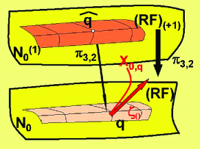
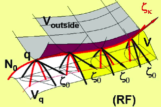
Figure 1. Solution Cauchy problem for $(RF)$, represented by the integral manifold $V$, envelopment manifold, generated by local solutions represented by manifolds $V_{q}$ tangent to $N_{0}$, $\forall q\in N_{0}$, and identified by means of $4$-dimensional integral planes $L_{\widehat{q}}$, for any $\widehat{q}\in N_{0}^{(1)}$. $V_{outside}\subset J{\it D}^{2}(E)$ represents a $4$-dimensional integral manifold, passing for $N_{0}$, but $V_{outside}\not\subset(RF)$. $V_{outside}$ can be deformed in $V$, taking fixed $N_{0}$. $(RF)$ and $(RF)_{+1}$ are represented with (yellow) frames, containing respectively $N_{0}$ and $N_{0}^{(1)}$.

Let us emphasize that, on $N_{0}$, (resp. $N_{1}$), the components of the characteristic vector field $\zeta_{0}$ in (48) are uniquely characterized by the metric $\gamma_{ij}$ and its derivatives up to sixth order. This proves that in order to characterize a solution of the Cauchy problem, identified by $N_{0}\subset(RF)$, it is necessary to consider the prolongation $(RF)_{+4}$, of $(RF)$, up to fourth order. Then the $4$-dimensional manifold $V=\bigcup_{t\in[0,\epsilon[}\phi_{t}(N_{0})\subset(RF)$, obtained by means of the local flow $\phi_{t}$ generated by $\zeta_{0}=\partial\phi$, is a local integral manifold, solution of the Cauchy problem identified by $N_{0}$. (So $\zeta_{0}$ is the characteristic vector field for such a solution.) Let us remark that such a solution does not necessitate to be smooth. In fact in this process we have used only the prolongation of $(RF)$ up to fourth-order, i.e., we have considered only the projections given in (49).

(49) $$\lx@xy@svg{\hbox{\raise 0.0pt\hbox{\kern 18.21149pt\hbox{\ignorespaces\ignorespaces\ignorespaces\hbox{\vtop{\kern 0.0pt\offinterlineskip\halign{\entry@#!@&&\entry@@#!@\cr&&&&\crcr}}}\ignorespaces{\hbox{\kern-18.21149pt\raise 0.0pt\hbox{\hbox{\kern 0.0pt\raise 0.0pt\hbox{\hbox{\kern 3.0pt\raise 0.0pt\hbox{$\textstyle{(RF)_{+4}\ignorespaces\ignorespaces\ignorespaces\ignorespaces}$}}}}}}}\ignorespaces\ignorespaces\ignorespaces\ignorespaces{}{\hbox{\lx@xy@droprule}}\ignorespaces{\hbox{\kern 42.21149pt\raise 0.0pt\hbox{\hbox{\kern 0.0pt\raise 0.0pt\hbox{\lx@xy@tip{1}\lx@xy@tip{-1}}}}}}{\hbox{\lx@xy@droprule}}{\hbox{\lx@xy@droprule}}{\hbox{\kern 42.21149pt\raise 0.0pt\hbox{\hbox{\kern 0.0pt\raise 0.0pt\hbox{\hbox{\kern 3.0pt\raise 0.0pt\hbox{$\textstyle{(RF)_{+3}\ignorespaces\ignorespaces\ignorespaces\ignorespaces}$}}}}}}}\ignorespaces\ignorespaces\ignorespaces\ignorespaces{}{\hbox{\lx@xy@droprule}}\ignorespaces{\hbox{\kern 102.63446pt\raise 0.0pt\hbox{\hbox{\kern 0.0pt\raise 0.0pt\hbox{\lx@xy@tip{1}\lx@xy@tip{-1}}}}}}{\hbox{\lx@xy@droprule}}{\hbox{\lx@xy@droprule}}{\hbox{\kern 102.63446pt\raise 0.0pt\hbox{\hbox{\kern 0.0pt\raise 0.0pt\hbox{\hbox{\kern 3.0pt\raise 0.0pt\hbox{$\textstyle{(RF)_{+2}\ignorespaces\ignorespaces\ignorespaces\ignorespaces}$}}}}}}}\ignorespaces\ignorespaces\ignorespaces\ignorespaces{}{\hbox{\lx@xy@droprule}}\ignorespaces{\hbox{\kern 163.05743pt\raise 0.0pt\hbox{\hbox{\kern 0.0pt\raise 0.0pt\hbox{\lx@xy@tip{1}\lx@xy@tip{-1}}}}}}{\hbox{\lx@xy@droprule}}{\hbox{\lx@xy@droprule}}{\hbox{\kern 163.05743pt\raise 0.0pt\hbox{\hbox{\kern 0.0pt\raise 0.0pt\hbox{\hbox{\kern 3.0pt\raise 0.0pt\hbox{$\textstyle{(RF)_{+1}\ignorespaces\ignorespaces\ignorespaces\ignorespaces}$}}}}}}}\ignorespaces\ignorespaces\ignorespaces\ignorespaces{}{\hbox{\lx@xy@droprule}}\ignorespaces{\hbox{\kern 223.48041pt\raise 0.0pt\hbox{\hbox{\kern 0.0pt\raise 0.0pt\hbox{\lx@xy@tip{1}\lx@xy@tip{-1}}}}}}{\hbox{\lx@xy@droprule}}{\hbox{\lx@xy@droprule}}{\hbox{\kern 223.48041pt\raise 0.0pt\hbox{\hbox{\kern 0.0pt\raise 0.0pt\hbox{\hbox{\kern 3.0pt\raise 0.0pt\hbox{$\textstyle{(RF)}$}}}}}}}\ignorespaces}}}}\ignorespaces. \textstyle{(RF)_{+4}\ignorespaces\ignorespaces\ignorespaces\ignorespaces} \textstyle{(RF)_{+3}\ignorespaces\ignorespaces\ignorespaces\ignorespaces} \textstyle{(RF)_{+2}\ignorespaces\ignorespaces\ignorespaces\ignorespaces} \textstyle{(RF)_{+1}\ignorespaces\ignorespaces\ignorespaces\ignorespaces} \textstyle{(RF)} \textstyle{(RF)_{+4}\ignorespaces\ignorespaces\ignorespaces\ignorespaces} \textstyle{(RF)_{+3}\ignorespaces\ignorespaces\ignorespaces\ignorespaces} \textstyle{(RF)_{+2}\ignorespaces\ignorespaces\ignorespaces\ignorespaces} \textstyle{(RF)_{+1}\ignorespaces\ignorespaces\ignorespaces\ignorespaces} \textstyle{(RF)}$$

However, we can obtain $V$ as a continuous manifold. In fact, let $g_{ij}(x^{\alpha})$ denote a local solution identified by $L_{\widehat{q}}=T_{q}V_{q}\subset T_{q}(RF)$, and $T_{q}N_{0}\subset L_{\widehat{q}}$. Then the time-like integral line $X_{0,q}\subset V_{q}$, tangent to $\zeta_{0}$, is represented by a local curve $\xi_{q}:[0,\epsilon_{q}[\subset\mathbb{R}\to(RF)$, given by the parametric equation (50) in $J{\it D}^{2}(E)$.

(50) $$\left\{\begin{array}[]{l}t\circ\xi=t\\ x^{k}\circ\xi=x^{k}(q)\\ g_{ij}\circ\xi=g_{ij}(t,x^{k}(q))\\ g_{ij,t}\circ\xi=\kappa R_{ij}(g(t,x^{k}))|_{x^{k}=x^{k}(q)}\\ g_{ij,h}\circ\xi=g_{ij,h}(t,x^{k})|_{x^{k}=x^{k}(q)}\\ g_{ij,hk}\circ\xi=g_{ij,hk}(t,x^{k})|_{x^{k}=x^{k}(q)}\\ g_{ij,th}\circ\xi=\kappa R_{ij,h}(g(t,x^{k}))|_{x^{k}=x^{k}(q)}\\ g_{ij,tt}\circ\xi=\kappa^{2}\sum_{0\leq|p|\leq 2}[(\partial g^{rs,p}.R_{ij})R_{rs,p}(g(t,x^{k}))]|_{x^{k}=x^{k}(q)}\\ \end{array}\right.$$

Since $\zeta_{0}$ continuously changes on $N_{0}$, it follows that curves $X_{0,q}$, $q\in N_{0}$, continuously change with $q\in N_{0}$, if the solutions $g_{ij}(t,x^{k})$ continuously change with $q\in N_{0}$ too. This is surely realized by the fact that points $q^{\prime}\in N_{0}$, near to $q$, come from points $\widehat{q}^{\prime}\in N_{0}^{(1)}$, near to $\widehat{q}$, if $\pi_{3,2}(\widehat{q})=q$. In fact, $N_{0}\cong N_{0}^{(1)}$ and $\pi_{3,2}(N_{0}^{(1)})=N_{0}$, thus $\pi_{3,2}|_{N_{0}^{(1)}}:N_{0}^{(1)}\to N_{0}$ is necessarily a continuous mapping. Moreover, we can continuously transform any (local) solution $g_{ij}(t,x^{k})$ of $(RF)$ into other ones by means of space-like (local) $1$-parameter group of diffeomorphisms $\phi_{\lambda}$, $\lambda\in[0,\epsilon[\subset\mathbb{R}$ of $M$. In fact, such transformations are locally represented by the following functions $\{t\circ\phi_{\lambda}=t,x^{k}\circ\phi_{\lambda}=\phi_{\lambda}^{k}(x^{i})\}$. As a by-product it follows that $(RF)$ is invariant under such transformations. In fact $(\phi_{\lambda}^{*}g)_{ij,t}-\kappa R_{ij}(\phi_{\lambda}^{*}g)=\phi_{\lambda}^{*}[g_{ij,t}-\kappa R_{ij}(g)]=0$. Thus we can continuously transform an integral manifold $V_{q}$, into other solutions along the space-like coordinate lines of $N_{0}$, passing for $q$ and identify, in the points $q^{\prime}\in N_{0}$, the time-like curves $X_{0,q^{\prime}}$ that result continuously transformed of $X_{0,q}$. In this way $V=\bigcup_{q\in N_{0}}X_{0,q}$ is a smooth manifold in a suitable tubular neighborhood of $N_{0}\times[0,\epsilon[$, that is the integral manifold of a metric $g_{ij}(t,x^{k})$, of class $C^{3}$, solution of the Ricci flow equation $(RF)$. This proves that the envelopment manifold $V$ is more regular than a viscosity solution.

In order to obtain a smooth solution of the Cauchy problem given by the integral manifold $N_{0}$ it is necessary to repeat the above process on the infinity prolongation $(RF)_{+\infty}\subset J{\it D}^{\infty}(E)$. In fact, also on $(RF)_{+\infty}$, the $3$-dimensional integral manifold $N_{0}\cong D^{\infty}\gamma(M)\equiv N_{0}^{(\infty)}\subset(RF)_{+\infty}$ is uniquely identified by $(M,\gamma)$, and identifies also a unique transversal time-like characteristic vector field $\zeta_{0}^{(\infty)}$, tangent to $(RF)_{+\infty}$. More precisely, $\zeta_{0}^{(\infty)}=\zeta_{0}+\sum_{|\alpha|>2}g_{ij,t\alpha}\partial g^{ij,\alpha}$, with $g_{ij,t\alpha}=\kappa R_{ij,\alpha}(\gamma)$, where $\alpha=0,1,2,3$.

The situation is resumed in the commutative diagram (51).

(51)

Similarly to what made in the Fourier’s heat equation, (see Example 3.21), we can prove that to the above solution one can associate weak-singular ones by using perturbations of the initial Cauchy data. In fact, if $V\subset(RF)$ is a regular solution passing for the integral manifold $N_{0}$, we can consider perturbations like solutions $\nu:\mathbb{R}\times M\to E$, of the linearized equation $(RF)[V]\subset J{\it D}^{2}(E)$. Since also $(RF)[V]$ is formally integrable and completely integrable, in neighborhoods of $N_{0}$ there exist perturbations. These deform $V$ (background solution) giving some new solutions $\widetilde{V}\subset(RF)$. Then $\widehat{V}\equiv V\bigcup\widetilde{V}\subset(RF)$ is a weak-singular solutions of the type just considered in Example 3.21 for the Fourier’s heat equation.

Now, for any of two of such integral manifolds, $N_{0}$ and $N_{1}$, we can find a smooth solution $V$ bording them, $V=N_{0}\mathop{\bigcup}\limits^{.}N_{1}$ iff their integral characteristic numbers are equal, i.e. all the conservation laws of $(RF)$ valued on them give equal numbers. By the way, under our assumptions we can consider $N_{0}$ and $N_{1}$ homotopy equivalent. Let $f:N_{1}\to N_{0}$ be such an homotopy equivalence. Let $\omega$ be any conservation law for $(RF)$. Then one has equation (52).

(52) $$<[N_{0}],[\omega]>=\int_{N_{0}}\omega=\int_{N_{1}}f^{*}\omega=<[N_{1}],[f^{*}\omega]>=<[N_{1}],[\omega]>=\int_{N_{1}}\omega.$$

So any possible integral characteristic number of $N_{0}$ must coincide with ones with $N_{1}$ and vice versa. Thus we can say, that with this meaning of admissibility (full admissibility hypothesis) on the Cauchy integral manifolds, one has $cry(RF)=0$, i.e., $(RF)$ becomes a $0$-crystal. Therefore there are not obstructions on the existence of smooth solutions $V$ of $(RF)$ bording $N_{0}$ and $N_{1}$, $\partial V=N_{0}\mathop{\bigcup}\limits^{.}N_{1}$, i.e., solutions without singular points.

This has as a by-product that $M$ and $S^{3}$ are homeomorphic manifolds. Hence the Poincaré conjecture is proved. With this respect we can say that this proof of the Poincaré conjecture is related to the fact that under suitable conditions of admissibility for the Cauchy integral manifolds, the Ricci-flow equation becomes a $0$-crystal PDE.

Example 3.25 (The d’Alembert equation $\frac{\partial^{2}\log f}{\partial x\partial y}=0$ on the $2$-dimensional torus).

The d’Alembert equation on a $2$-dimensional manifold $M$ can be encoded by a second-order differential equation

(53) $$(d^{\prime}A)_{2}\subset J{\it D}^{2}(W):\left\{uu_{xy}-u_{x}u_{y}=0\right\}$$

with $W\equiv M\times\mathbb{R}$. In [60] we have calculated the integral bordism groups of such an equation. In particular for $M=T^{2}$, the $2$-dimensional torus, one has $\Omega_{1}^{(d^{\prime}A)_{2}}\cong\mathbb{Z}_{2}\bigoplus\mathbb{Z}_{2}$. Taking into account Example 2.20 we see that $\Omega_{1}^{(d^{\prime}A)_{2}}$ is isomorphic to the crystal group $G(2)=\mathbb{Z}^{2}\rtimes D_{4}=p4m$. Therefore, $(d^{\prime}A)_{2}$ on $T^{2}$ is an extended crystal PDE, with crystal dimension $2$.

Example 3.26 (The Tricomi equation on $2$-dimensional manifolds).

In [60] we have considered the integral bordism groups of the Tricomi equation $(T)$:

(54) $$(T)\subset J{\it D}^{2}(W):\left\{u_{yy}-yu_{xx}=0\right\}$$

defined on a $2$-dimensional manifold $M$, i.e. with $W\equiv M\times\mathbb{R}$. For example, on the $2$-dimensional torus $T^{2}$ one has $\Omega_{1}^{(T)}\cong{\mathbb{Z}}_{2}\oplus{\mathbb{Z}}_{2}$. Furthermore on ${\mathbb{R}}P^{2}$ we obtains $\Omega_{1}^{(T)}\cong{\mathbb{Z}}_{2}$. Thus the Tricomi equation on $T^{2}$, (resp. $S^{2}$), is an extended crystal PDE with crystal group $p4m$, (resp. $p2$), and crystal dimension $2$, (resp. $2$).

Example 3.27 (The Navier-Stokes PDE).

The non isothermal Navier-Stokes equation can be encoded by a second order PDE $\widehat{(NS)}\subset J{\it D}^{2}(W)$ on a $9$-dimensional affine fiber bundle $\pi:W\to M$ on the Galilean space-time $M$. In Tab. 1 is reported its polynomial differential structure.

Table 1. Completely integrable Navier-Stokes equation: $\widehat{(NS)}\subset J{\it D}^{2}(W)$ defined by differential polynomials.

${\rm(A)}:F^{0}\equiv\dot{x}^{k}G^{j}_{jk}+\dot{x}^{i}_{s}\delta^{s}_{i}=0$ ($\scriptstyle F^{0}\in A[\dot{x}^{k},\dot{x}^{i}_{s}]$)

(continuity equation)

${\rm(B)}:F^{0}_{\alpha}\equiv\dot{x}^{k}(\partial x_{\alpha}.G^{j}_{jk})+\dot{x}^{k}_{\alpha}G^{j}_{jk}+\dot{x}^{i}_{s\alpha}\delta^{s}_{i}=0$ ($\scriptstyle F^{0}_{\alpha}\in A[\dot{x}^{k},\dot{x}^{i}_{\alpha},\dot{x}^{i}_{s\alpha}]$)

(first prolonged continuity equation)

${\rm(C)}:F^{j}\equiv\dot{x}^{s}R^{j}_{s}+\dot{x}^{s}\dot{x}^{i}\rho G^{j}_{is}+\dot{x}^{s}\dot{x}^{j}_{s}\rho+\rho\dot{x}^{j}_{0}+\dot{x}^{k}_{s}S^{js}_{k}+\dot{x}^{j}_{is}T^{is}$

$+p_{i}g^{ij}+\rho(\partial x_{i}.f)g^{ij}=0$ ($\scriptstyle F^{j}\in A[\dot{x}^{s},\dot{x}^{i}_{s},\dot{x}^{j}_{is},p_{i}]$)

(motion equation)

${\rm(D)}:F^{4}\equiv\theta_{0}\rho C_{p}+\rho C_{p}\dot{x}^{k}\theta_{k}+\theta_{is}\overline{E}^{is}+\dot{x}^{k}\dot{x}^{p}W_{kp}+\dot{x}^{k}\dot{x}^{s}_{p}{\overline{W}}^{p}_{ks}+\dot{x}^{k}_{i}\dot{x}^{s}_{p}Y^{ip}_{ks}=0$

($\scriptstyle F^{4}\in A[\dot{x}^{k},\dot{x}^{s}_{p},\theta_{0},\theta_{k},\theta_{is}]$) (energy equation)

Functions belonging to $\scriptstyle A\subset\mathbb{R}[[x^{1},x^{2},x^{3}]]$

$\scriptstyle R^{j}_{s}\equiv\chi[(\partial x_{p}.G^{j}_{is})+G^{j}_{pq}G^{q}_{is}-G^{q}_{pi}G^{j}_{qs}]g^{pi}$

$\scriptstyle S^{js}_{k}\equiv\chi[2G^{j}_{ik}g^{si}-G^{s}_{qi}\delta^{j}_{k}g^{qi}]$

$\scriptstyle T^{is}\equiv\chi g^{is}=T^{si}$

$\scriptstyle\overline{E}^{is}\equiv-\nu g^{is}=\overline{E}^{si}$

$\scriptstyle W_{kp}\equiv-\chi G^{a}_{jk}G^{b}_{sp}(g_{ba}g^{sj}+\delta^{j}_{b}\delta^{s}_{a})=-2\chi G^{s}_{bk}G^{b}_{sp}=W_{pk}$

$\scriptstyle{\overline{W}}^{p}_{ks}\equiv-2\chi[G^{j}_{ik}g_{js}g^{ip}+G^{p}_{sk}]=-4\chi G^{p}_{sk}={\overline{W}}^{p}_{sk}$

$\scriptstyle Y^{ip}_{ks}\equiv-\chi[g_{ks}g^{ip}+\delta^{p}_{k}\delta^{i}_{s}]=Y^{pi}_{sk}$

$\scriptstyle 0\leq\alpha\leq 3,\hskip 2.0pt1\leq i,j,k,p,s\leq 3.\hskip 2.0pt(\partial x_{0}.G^{j}_{jk})=0$.

There $\{x^{\alpha},\dot{x}^{k},p,\theta\}$ are fibered coordinates on $W$, adapted to the inertial frame, and $G^{k}_{ij}$ are the canonical connection symbols on $M$. Furthermore $A\subset\mathbb{R}[[x^{1},x^{2},x^{3}]]$ is the algebra of real valued analytic functions of $(x^{k})$. We have proved in Refs.[55, 62] that the singular integral bordism groups of such an equation are trivial, i.e., $\Omega^{\widehat{(NS)}}_{3,s}\cong\Omega^{\widehat{(NS)}}_{3,w}\cong 0$. Furthermore, with respect to the notation used in diagram (26), one has that for the integral bordism group for smooth solutions: $\Omega^{\widehat{(NS)}}_{3}\cong K^{\widehat{(NS)}}_{3,w}$. Thus we can conclude that the Navier-Stokes equation is an extended $0$-crystal PDE, but not a $0$-crystal, i.e. $cry\widehat{(NS)}\not=0$. Note that if we consider admissible only all the Cauchy integral manifolds $X\subset\widehat{(NS)}$ such that all their integral characteristic numbers are zero, (full admissibility hypothesis), it follows that $cry\widehat{(NS)}=0$. So, under this condition, $\widehat{(NS)}$ becomes a $0$-crystal PDE.

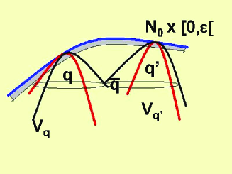
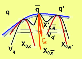
Figure 2. Construction of envelopment solution $V$ for Cauchy problem $N_{0}^{(\infty)}\subset\widehat{(NS)}_{+\infty}$, on the infinity prolongation of $\widehat{(NS)}_{+\infty}$ of $\widehat{(NS)}$. One has $V=\bigcup_{q\in N_{0}^{(\infty)}}X_{0,q}$, with $X_{0,q}$ the unique time-like curve passing for $q$, tangent to the vector $\zeta_{0}(q)$ and contained in the unique analytic solution passing for $q$.

Let us emphasize that, similarly to the Ricci flow equation, we can identify $3$-dimensional space-like smooth integral manifold $N_{0}\subset\widehat{(NS)}_{t}$, such that $N_{0}\cong M_{t}$, via the canonical projection $\pi_{2}:J{\it D}^{2}(W)\to M$, with some smooth space-like section $s_{t}:M_{t}\subset M\to W_{t}\subset W$, of the configuration bundle $\pi:W\to M$. In fact, all the coordinates in $\widehat{(NS)}$, containing time-derivatives, can be expressed by means of the other derivatives containing only space coordinates. (Warn for equation $\widehat{(NS)}$! Even if there are not restrictions on the time derivatives of pressure, between space derivatives of pressure arise some constraints, as well as there are constraints between space derivatives of velocity components, hence sections $s_{t}$ that identify above considered integral manifolds, are not arbitrary ones. For details see below.) Then we can solve the corresponding Cauchy problem applying Lemma 3.20, similarly to what made in the Ricci flow equation. It is useful to remark that in order to build envelopment solutions $V=\bigcup_{q\in N_{0}}X_{0,q}$, it does not necessitate to handle with PDE’s that admit any space-like symmetry. This of course does not happen for any smooth boundary value problem in $\widehat{(NS)}$. With this respect, it is useful also to underline that the popular request to maximize entropy cannot be an enough criterion to realize a smooth envelopment solution. (For complementary results on variational problems constrained by the Navier-Stokes equation see [62].) The existence of such a smooth envelopment manifold, can be proved by working on $\widehat{(NS)}_{+\infty}$. In fact, let $q,q^{\prime}\in N_{0}^{(\infty)}\subset\widehat{(NS)}_{+\infty}$, and let $V_{q}$ and $V_{q^{\prime}}$ be two smooth solutions passing for the initial conditions $q$ and $q^{\prime}$ respectively. We claim that their time-like integral curves $X_{0,q}$ and $X_{0,q^{\prime}}$ cannot intersect for suitable short times, i.e., $t\in[0,\epsilon[$, if $q\not=q^{\prime}$. Really if $\bar{q}\in V_{q}\bigcap V_{q^{\prime}}\not=\emptyset$, then $T_{\bar{q}}V_{q}=T_{\bar{q}}V_{q^{\prime}}=(\mathbf{E}_{\infty})_{\bar{q}}$. This means that in such a point $\bar{q}$, $V_{q}$ and $V_{q^{\prime}}$ must have a contact of infinity order with the Navier-Stokes equation and between them. We can assume that $\bar{q}$ is outside a suitable tubular neighborhood $N_{0}^{(\infty)}\times[0,\epsilon[$ of $N_{0}^{(\infty)}$, otherwise we should admit that $\bar{q}\in N_{0}^{(\infty)}$. In this last case $V_{q}$ and $V_{q^{\prime}}$ should have in $\bar{q}$ time-like curves $X_{0,\bar{q}}$ and $X^{\prime}_{0,\bar{q}}$, transversal to $N_{0}^{(\infty)}$, and with a common tangent vector $\zeta_{0}(\bar{q})$. Furthermore , $V_{q}$ and $V_{q^{\prime}}$ should be tangent to $N_{0}^{(\infty)}$ at $\bar{q}$: $T_{\bar{q}}V_{q}=T_{\bar{q}}V_{q^{\prime}}=(\mathbf{E}_{\infty})_{\bar{q}}\supset T_{\bar{q}}N_{0}^{(\infty)}$. Let us assume that in a suitable neighborhood $N_{0}^{(\infty)}\times[0,\epsilon[$, the manifold $V_{q}$ identifies two separated pieces, say and $V_{q|1}$ and $V_{q|2}$, tangent to $N_{0}^{(\infty)}$ at $q$ and $\bar{q}$, respectively. In other words $V_{q}\bigcap N_{0}^{(\infty)}\times[0,\epsilon[=V_{q|1}\bigcup V_{q|2}$. (If this condition is not satisfied, then $V_{q}$ is necessarily a smooth solution of the Cauchy problem at least in a subset $Y\subset N_{0}^{(\infty)}$. Then we can write $V=V_{1}\bigcup V_{2}\equiv\{\bigcup_{q\in Y}X_{0,q}\}\bigcup\{\bigcup_{q\in Z}X_{0,q}\}$, $Z\equiv N_{0}^{(\infty)}\setminus Y$, and we can continue to similarly discuss about the $V_{2}$-part of $V$.) Then, for the time-like coordinate lines $X_{0,q|1}$ and $X_{0,q|2}$, one has $X_{0,q|1}\bigcap X_{0,q|2}=\emptyset$ in $N_{0}^{(\infty)}\times[0,\epsilon[$. The same circumstance can be verified between $V_{q^{\prime}}$ and $V_{\bar{q}}$, eventually by reducing $\epsilon$. This proves that taking $\epsilon$ little enough, we can consider $V\equiv\bigcup_{q\in N_{0}^{(\infty)}}X_{0,q}\subset\widehat{(NS)}_{+\infty}$, a fiber bundle over $N_{0}^{(\infty)}$ that is a $4$-dimensional integral manifold representing a local solution of the Cauchy problem identified by the smooth $3$-dimensional integral manifold $N_{0}\subset\widehat{(NS)}$. (See Fig. 2.) On $V$ we can recognize a natural smooth fiber bundle structure. In fact, since $\widehat{(NS)}$ is an analytic equation and any point $q\in N_{0}^{(\infty)}$ identifies an analytic solution in a suitable neighborhood $U$ of $p\equiv\pi_{\infty}(q)\in M$, it follows that if two such solutions $s$ and $s^{\prime}$ are defined at $q\in N_{0}^{(\infty)}$ they should coincide in a suitable neighborhood of $p$, denote again it by $U$. Then we can assume that $s$ and $s^{\prime}$ coincide also in $\Omega\equiv\pi_{\infty}^{-1}(U)\bigcap N_{0}^{(\infty)}$. Therefore, we can cover $N_{0}^{(\infty)}$ by means of a covering set $\{\Omega_{\alpha}\}_{\alpha\in J}$, where each $\Omega_{\alpha}$ is such that if $q,q^{\prime}\in\Omega_{\alpha}$, the corresponding analytic solutions $s$ and $s^{\prime}$ are well defined in $U_{\alpha}\subset M$. In this way each time-like curve $X_{0,q}$ is uniquely identified for $q\in\Omega_{\alpha}$. Then we can define smooth functions (transition functions) $\psi_{\alpha\beta}:\Omega_{\alpha}\bigcap\Omega_{\beta}\to\mathbb{R}^{\bullet}\equiv\mathbb{R}\setminus\{0\}$, by $\tau_{\alpha}=\psi_{\alpha\beta}\tau_{\beta}$, where $\tau_{\alpha}$ are nowhere vanishing sections of $V\to N_{0}^{(\infty)}$ on $\Omega_{\alpha}\subset N_{0}^{(\infty)}$. These functions satisfy the following three conditions: (a) $\psi_{\alpha\alpha}=1$; (b) $\psi_{\alpha\beta}=\psi_{\beta\alpha}$; (c) $\psi_{\alpha\beta}\psi_{\beta\gamma}\psi_{\gamma\alpha}=1$ on $\Omega_{\alpha}\bigcap\Omega_{\beta}\bigcap\Omega_{\gamma}$ (cocycle condition). This is enough to claim that the line bundle $V\to N_{0}^{(\infty)}$ has a smooth structure. Let us emphasize that Lemma 3.20 can be applied here also to $3$-dimensional space-like smooth Cauchy integral manifolds $N\subset\widehat{(NS)}_{t}$, that are diffeomorphic to their projections $Y\equiv\pi_{2,0}(N)\subset W_{t}$, but are not necessarily holonomic images of smooth sections of $\pi:W\to M$. In fact, by using the embeddings $N\subset\widehat{(NS)}\subset J{\it D}^{2}(W)\subset J^{2}_{4}(W)$, we can repeat above construction to build smooth envelopment solutions of the Cauchy problem $N^{(\infty)}\subset\widehat{(NS)}_{+\infty}\subset J^{\infty}_{4}(W)$. Really, any smooth $3$-dimensional space-like submanifold $Y\subset W_{t}$, identified by a space-like smooth integral manifold $Z\subset\widehat{(NS)}_{+\infty}\subset J^{\infty}_{4}(W)$, such that $Z\cong Y$, via the canonical projection $\pi_{\infty,0}:J^{\infty}_{4}(W)\to W$, can be locally identified by some smooth implicit functions $\{f_{I}(x^{k},y^{j})=0\}_{1\leq I\leq 5}$, with Jacobian matrix of rank five, where $\{x^{k},y^{j}\}_{1\leq k\leq 3;1\leq j\leq 5}$ are coordinates in the $8$-dimensional affine space $W_{t}$, and we write $Z=Y^{(\infty)}$. Then, as a by-product we get also a cohomology criterion to classify envelopment solutions according to the first cohomology space $H^{1}(N_{0},\mathbb{Z}_{2})$. In fact, a line bundle $V\to N_{0}^{(\infty)}$ is classified by the first Stiefel-Whitney class of $V$, that belongs to $H^{1}(N_{0}^{(\infty)},\mathbb{Z}_{2})\cong H^{1}(N_{0},\mathbb{Z}_{2})$. The classifying space is $\mathbb{R}P^{\infty}$ and the universal principal bundle is $S^{\infty}\to\mathbb{R}P^{\infty}\equiv S^{\infty}/\mathbb{Z}_{2}\cong\mathbb{R}^{\infty}/\mathbb{R}^{\bullet}\cong Gr_{1}(\mathbb{R}^{\infty})$, where $Gr_{1}(\mathbb{R}^{\infty})$ denotes the Grassmannian of $1$-dimensional vector subspaces in $\mathbb{R}^{\infty}$, and the nonzero element of $\mathbb{Z}_{2}$ acts by $v\mapsto-v$. Since $S^{\infty}$ is contractible one has $\pi_{i}(S^{\infty})\cong\pi_{i}(\mathbb{R}P^{\infty})=0$, $i>1$ and $\pi_{1}(\mathbb{R}P^{\infty})\cong\mathbb{Z}_{2}$. $\mathbb{R}P^{\infty}$ is the Eilenberg-Maclane space $K(\mathbb{Z}_{2},1)$ [58]. Hence $[N_{0},Gr_{1}]\cong H^{1}(N_{0};\mathbb{Z}_{2})$, $f\mapsto f^{*}\mu$, where $\mu$ is the generator of $H^{1}(\mathbb{R}P^{\infty};\mathbb{Z}_{2})\cong\mathbb{Z}_{2}$. Since one has the bijection $[N_{0};Gr_{1}]\to\mathbf{V}_{1}(N_{0})$, where $\mathbf{V}_{1}(N_{0})$ denotes the set of $1$-dimensional vector bundles over $N_{0}$, we get the bijection $w_{1}:\mathbf{V}_{1}(N_{0})\to H^{1}(N_{0};\mathbb{Z}_{2})$ that is just the Stiefel-Whitney class for line bundles over $N_{0}^{(\infty)}$. In conclusion an envelopment solution $V\supset N$, of an admissible Cauchy integral manifolds $N\subset\widehat{(NS)}$, can be identified with some cohomology class of $H^{1}(N;\mathbb{Z}_{2})$. In particular $V$ is orientable iff its first Stiefel-Whitney cohomology class $w_{1}(V)=0$. Of course does not necessitate that all cohomology classes of $H^{1}(N;\mathbb{Z}_{2})$ should be represented by some envelopment solution $V$ passing for $N$. However, when this happens we say that $N$ is a wholly cohomologic Cauchy manifold of $\widehat{(NS)}$. This is surely the case when $N\simeq D^{3}$, i.e., when the space-like, smooth, $3$-dimensional, integral manifold $N$ is homotopy equivalent to the $3$-dimensional disk $D^{3}$. In fact in such a case $H^{1}(N;\mathbb{Z}_{2})=0$, hence there is an unique cohomology type of envelopment solution passing for $N^{(\infty)}$, (or $N$), the orientable one. Therefore, in such a case $N$ is a wholly cohomologic Cauchy manifold. For example, when $N$ is identified by a smooth space-like section $s_{t}:M_{t}\subset M\to W_{t}\subset W$, $N$ is a wholly cohomologic Cauchy manifold. It is important to remark also that, fixed some smooth Cauchy problem $N\subset\widehat{(NS)}$, it does not necessitate that a local smooth solution $V\epsilon$ should be unique. In fact, even if the Cartan distribution $\mathbf{E}_{\infty}\subset\widehat{(NS)}_{+\infty}$, is a $4$-dimensional involutive distribution, the manifold $\widehat{(NS)}$, is not finite dimensional, therefore for any point $q\in\widehat{(NS)}$ pass infinity $4$-dimensional integral manifolds tangent to $(\mathbf{E}_{\infty})_{q}\subset T_{q}(\widehat{(NS)}_{+\infty})$. However, we can see that if there are two smooth solutions $V_{\epsilon},V^{\prime}_{\epsilon}\subset\widehat{(NS)}_{+\infty}$ for a fixed smooth Cauchy problem $N\subset\widehat{(NS)}$, their Stiefel-Whitney classes must coincide with a same cohomology class of $H^{1}(N,\mathbb{Z}_{2})$. In fact, let us denote by $\mathbf{N}_{\infty}(N)_{\epsilon}$ the integral $\epsilon$-normal bundle of $N^{(\infty)}$, i.e., $\mathbf{N}_{\infty}(N)_{\epsilon}\equiv\bigcup_{q\in N^{(\infty)}}\mathbf{N}_{\infty}(N)_{\epsilon,q}$, with $\mathbf{N}_{\infty}(N)_{\epsilon,q}\equiv((\mathbf{E}_{\infty})_{q}/T_{q}N)_{\epsilon}\equiv\{[0,\epsilon[\zeta_{0}(q)\}$. Then one has the canonical isomorphism of line bundles over $N^{(\infty)}$: $\mathbf{N}_{\infty}(N)_{\epsilon}\cong V_{\epsilon}$, $\lambda\zeta_{0}(q)\mapsto X_{0,q}(\lambda)$, $\lambda\in[0,\epsilon[$. A similar isomorphism can be recognized between $\mathbf{N}_{\infty}(N)_{\epsilon}$ and $V^{\prime}_{\epsilon}$, taking into account that also $V^{\prime}_{\epsilon}$ can be considered a line bundle: $V^{\prime}_{\epsilon}\equiv\bigcup{q\in N^{(\infty)}}X^{\prime}_{0,q}$. This proves that must necessarily be $\omega_{1}(V_{\epsilon})=\omega_{1}(\mathbf{N}_{\infty}(N)_{\epsilon})=\omega_{1}(V^{\prime}_{\epsilon})$.

So we have shown that any space-like smooth $3$-dimensional integral manifold $N\subset\widehat{(NS)}$ that is diffeomorphic to its projection on $M_{t}\subset M$, (for some $t$), via the canonical projection $\pi_{2}:J{\it D}^{2}(W)_{t}\to M_{t}$, or is diffeomorphic to its projection on $W_{t}$, via the canonical projection $\pi_{2,0}:J{\it D}^{2}(W)_{t}\to W_{t}$, admits smooth solutions, $V\supset N$. Since such integral manifolds (Cauchy manifolds) are not arbitrary ones, but satisfy some constraints, here we shall explicitly prove that such Cauchy manifolds exist. From Tab. 1 we can write $\widehat{(NS)}$ in the form reported in (55)

(55)

From the prolongation of equation (55)(C) with respect to space coordinates $x^{k}$, we get

(56) $$\left\{\begin{array}[]{ll}\hbox{\rm(C)}_{q}\hskip 2.0pt\dot{x}^{j}_{0q}&=\frac{1}{\rho}\left[-\dot{x}^{s}_{q}R^{j}_{s}-\dot{x}^{s}_{q}R^{j}_{s,q}-2\dot{x}^{s}_{q}\dot{x}^{i}\rho G^{j}_{is}-\dot{x}^{s}\dot{x}^{i}\rho G^{j}_{is,q}-\dot{x}^{s}_{q}\dot{x}^{j}_{s}\rho-\dot{x}^{s}\dot{x}^{j}_{sq}\rho\right.\\ &\left.-\dot{x}^{k}_{sq}S^{js}_{k}-\dot{x}^{k}_{s}S^{js}_{k,q}-\dot{x}^{j}_{isq}T^{is}-\dot{x}^{j}_{is}T^{is}_{,q}-p_{iq}g^{ij}-p_{i}g^{ij}_{,q}\right.\\ &\left.-\rho(\partial x_{q}\partial x_{i}.f)g^{ij}-\rho(\partial x_{i}.f)g^{ij}_{,q}\right]\\ &\equiv H^{j}_{,q}\in A[[\dot{x}^{k},\dot{x}^{k}_{h},\dot{x}^{k}_{rs},\dot{x}^{k}_{rsq},p_{i},p_{iq}]]\\ \end{array}\right.$$

By using equations (55)(C) and (56)$(C)_{q}$, we can rewrite equation (55)$(B)_{0}$ in the form reported in (57).

(57) $$\hbox{\rm(E)}\hskip 10.0ptG^{j}_{jk}H^{k}(x^{k},\dot{x}^{s},\dot{x}^{s}_{k},\dot{x}^{s}_{hk},p_{i})+H^{s}_{,s}(x^{k},\dot{x}^{s},\dot{x}^{s}_{k},\dot{x}^{s}_{hk},\dot{x}^{s}_{hkq},p_{i},p_{iq})=0.$$

Therefore, the parametric equations of a space-like integral analytic $3$-dimensional manifold $N\subset\widehat{(NS)}$, diffeomorphic to $M_{t}$, are given in (58).

(58)

where $v^{j}=\dot{x}^{j}(x^{k})$ are solutions of the continuity equation (55)(A). Therefore, equation (55)(A) can be considered a first order equation on the fiber bundle $E_{t}\equiv M_{t}\times\mathbf{I}\to M_{t}$, reported in (59).

(59) $$E_{1}\subset J{\it D}(E_{t}):\hskip 5.0pt\{\dot{x}^{k}G^{j}_{jk}+\dot{x}^{s}_{s}=0\}.$$

One can see that $E_{1}$ is an involutive, formally integrable and completely integrable PDE. In fact, one has

$$\scalebox{0.8}{$\framebox{$\dim(E_{1})_{+1}=29$}=\framebox{$\dim E_{1}=14$}+\framebox{$\dim(g_{1})_{+1}=15$}$},$$

hence the mapping $(E_{1})_{+1}\to E_{1}$ is surjective. Furthermore, we get

$$\scalebox{0.8}{$\framebox{$\dim(g_{1})_{+1}=15$}=\framebox{$\dim g_{1}=8$}+\framebox{$\dim(g_{1})^{(1)}=5$}+\framebox{$\dim(g_{1})^{(2)}=2$}+\framebox{$\dim(g_{1})^{(3)}=0$}$}.$$

This is enough to state that $g_{1}$ is an involutive symbol. Therefore, $E_{1}$ is formally integrable and, since it is analytic it is also completely integrable. As a by-product, we get that for any analytic solution $\dot{x}^{k}=\dot{x}^{k}(x^{i})$ of $E_{1}$, we can write:

(60) $$\left\{\begin{array}[]{ll}\dot{x}^{j}_{0}=A^{j}(x^{s})-g^{ij}p_{i}\\ \dot{x}^{j}_{q0}=A^{j}(x^{s})_{,q}-\frac{1}{\rho}g^{ij}p_{iq}-\frac{1}{\rho}g^{ij}_{,q}p_{i}\\ \end{array}\right.$$

where $A^{j}=A^{j}(x^{s})$ are suitable analytic functions. So equation (57)(E) can be rewritten as a second order equation $E_{2}$ for a function $p=p(x^{k})$ as section of the trivial fiber bundle $F_{t}\equiv M_{t}\times\mathbb{R}\to M_{t}$:

(61) $$E_{2}\subset J{\it D}^{2}(F_{t}):\hskip 5.0pt\{g^{is}p_{is}+p_{i}C^{i}(x^{k})-B(x^{k})=0\}$$

where $C^{i}$ and $B$ are given analytic functions of $x^{k}$. This is an involutive, formally integrable PDE, hence it is completely integrable, since it is analytic. In fact,

$$\scalebox{0.8}{$\framebox{$\dim(E_{2})_{+1}=19$}=\framebox{$\dim(E_{2})=12$}+\framebox{$\dim(g_{2})_{+1}=7$}$}.$$

Therefore, the map $(E_{2})_{+1}\to E_{2}$ is surjective. Furthermore,

$$\scalebox{0.8}{$\framebox{$\dim(g_{2})_{+1}=7$}=\framebox{$\dim(g_{2})=5$}+\framebox{$\dim(g_{2})^{(1)}=2$}+\framebox{$\dim(g_{2})^{(2)}=0$}$},$$

hence $g_{2}$ is an involutive symbol. This concludes the proof. Thus, for any point $q\in E_{1}$, pass solutions of the continuity equation, and fixing a point $q$ on the infinity prolongation $(E_{1})_{+\infty}$, one identifies an analytic solution defined in a suitable neighborhood of $p\equiv\pi_{\infty}(q)\in M_{t}$. (Of course also for equation $E_{1}$ we can identify smooth solutions by solving lower dimension Cauchy problems, by means of Lemma 3.20, i.e., by using envelopment solutions.) Similar considerations can be applied to the equation $E_{2}$ to identify analytic and smooth solutions of the pressure functions $p=p(x^{k})$. This assures that one can identify space-like smooth Cauchy manifolds in $\widehat{(NS)}$, that are diffeomorphic with their canonical projections on $W_{t}$, for any time $t$.

In [62] it is proved that the set of full admissible Cauchy integral manifolds is not empty. This result gives us a general criterion to characterize global smooth solutions of the Navier-Stokes equation and completely solves the well-known problem on the existence of global smooth solutions of the Navier-Stokes equation. (For complementary characterizations of the Navier-Stokes equation see also [62, 67, 68, 69, 70, 71]. There a geometric method to study stability of PDE’s and their solutions, related to integral and quantum bordism groups of PDE’s, has been introduced, and applied to the Navier-Stokes equation too.)

4. EXTENDED CRYSTAL SINGULAR PDE’s

Singular PDE’s can be considered singular submanifolds of jet-derivative spaces. The usual formal theory of PDE’s works, instead, on smooth or analytic submanifolds. However, in many mathematical problems and physical applications, it is necessary to work with singular PDE’s. (See, e.g., the book by Gromov [25] where he talks of ”partial differential relations”, i.e., subsets of jet-derivative spaces.) So it is useful to formulate a general geometric theory for such more general mathematical structures. On the other hand in order to build a formal theory of PDE’s it is necessary to assume some regularity conditions. So a geometric theory of singular PDE’s must in some sense weak the regularity conditions usually adopted in formal theory and admit existence of subsets where these regularity conditions are not satisfied. With this respect, and by using our formulation of geometric theory of PDE’s and singular PDE’s, we study criteria to obtain global solutions of singular PDE’s, crossing singular points. In particular, some applications concerning singular MHD-PDE’s, encoding anisotropic incompressible nuclear plasmas dynamics, are given following some our recent works on this subject. The origin of singularities comes from the fact that there are two regions corresponding to different components PDE’s having different Cartan distributions with different dimensions. However, by considering their natural embedding into a same PDE, we can build physically acceptable solutions, i.e., satisfying the second principle of the thermodynamics, and that cross the nuclear critical zone of nuclear energy production. A characterization of such solutions by means of algebraic topological methods is given also.

The main result of this section is Theorem 4.30 that relates singular integral bordism groups of singular PDE’s to global solutions passing through singular points, and Example 4.33 that for some MHD-PDE’s characterizes global solutions crossing the nuclear critical zone and satisfying the entropy production energy thermodynamics condition.

Let us, now, resume some fundamental definitions and results on the geometry of PDE’s in the category of commutative manifolds, emphasizing some our recent results on the algebraic geometry of PDE’s, that allowed us to characterize singular PDE’s.

Definition 4.1 (Algebraic formulation of PDE’s).

Let $\pi:W\to M$ be a smooth fiber bundle, $\dim W=m+n$, $\dim M=n$. We denote by $J^{k}_{n}(W)$ the space of all $k$-jets of submanifolds of dimension $n$ of $W$ and by $J^{k}(W)$ the $k$-jet-derivative space of sections of $\pi$. Furthermore we denote by $J{\it D}^{k}(W)$ the $k$-jet-derivative space for sections of $\pi$. One has $J{\it D}^{k}(W)\cong J^{k}(W)\subset J^{k}_{n}(W)$. $J^{k}(W)$ is an open subset of $J^{k}_{n}(W)$. Let ${\mathfrak{A}}_{k}$ be the sheaf of germs of differentiable functions $J{\it D}^{k}(W)\rightarrow\mathbb{R}$. It is a sheaf of rings, but also a sheaf of $\mathbb{R}$-modules. A subsheaf of ideals ${\mathfrak{B}}_{k}$ of ${\mathfrak{A}}_{k}$ that is also a subsheaf of $\mathbb{R}$-modules is a PDE of order k on the fiber bundle $\pi:W\rightarrow M$. A regular solution of ${\mathfrak{B}}_{k}$ is a section $s:M\rightarrow W$ such that $f\circ D^{k}s=0,\forall f\in{\mathfrak{B}}_{k}$. The set of integral points of ${\mathfrak{B}}_{k}$ (i.e., the zeros of ${\mathfrak{B}}_{k}$ on $J{\it D}^{k}(W)$ is denoted by $J({\mathfrak{B}}_{k})$. The first prolongation $({\mathfrak{B}}_{k})_{+1}$ of ${\mathfrak{B}}_{k}$ is defined as the system of order $k+1$ on $W\rightarrow M$, defined by the $f\circ\pi_{k,k-1}$ and $f^{(1)}$, where $f^{(1)}$ on $D^{k+1}s(p)$ is defined by $f^{(1)}(D^{k+1}s(p))=(\partial x_{\alpha}.(f\circ D^{k}s(p)))$. In local coordinates $(x^{\alpha},y^{j},y^{j}_{\alpha})$ the formal derivative $f^{(1)}$ is given by $f^{(1)}(x^{\alpha},y^{j},y^{j}_{\alpha})=(\partial x_{\alpha}.f)+\sum_{[\beta]\leq k}y^{j}_{\beta\alpha}(\partial y^{\beta}_{j}.f)$. The system ${\mathfrak{B}}_{k}$ is said to be involutive at an integral point $q\in J{\it D}^{k}(W)$ if the following two conditions are satisfied: (i) ${\mathfrak{B}}_{k}$ is a regular local equation for the zeros of ${\mathfrak{B}}_{k}$ at q (i.e., there are local sections $F_{1},...,F_{t}\in\Gamma(U,{\mathfrak{B}}_{k})$ of ${\mathfrak{B}}_{k}$ on an open neighborhood $U$ of $q$, such that the integral points of ${\mathfrak{B}}_{k}$ in $U$ are precisely the points $q^{\prime}$ for which $F_{j}(q^{\prime})=0$ and $dF_{1}\wedge\cdots\wedge dF_{t}(q)\not=0$, that is $F_{1},\cdots,F_{t}$ are linearly independent at $q;$ and (ii) there is a neighborhood $U$ of $q$ such that $\pi^{-1}_{k+1,k}(U)\bigcap J(({\mathfrak{B}}_{k})_{+1})$ is a fibered manifold over $U\bigcap J({\mathfrak{B}}_{k})$ (with projection $\pi_{k+1,k})$. For a system ${\mathfrak{B}}_{k}$ generated by linearly independent Pfaffian forms $\theta^{1},\cdots,\theta^{k}$ (i.e., a Pfaffian system) this is equivalent to the involutiveness defined for distributions.

Theorem 4.2 ([34]).

Let ${\mathfrak{B}}_{k}$ be a system defined on $J{\it D}^{k}(W)$, and suppose that ${\mathfrak{B}}_{k}$ is involutive at $q\in J({\mathfrak{B}}_{k})$. Then, there is a neighborhood $U$ of $q$ satisfying the following. If $\widetilde{q}\in J(({\mathfrak{B}}_{k})_{+s})$ and $\pi_{k+s,k}(\widetilde{q})$ is in $U$, then there is a regular solution $s$ of ${\mathfrak{B}}_{k}$ defined on a neighborhood $p=\pi_{k+s,-1}(\widetilde{q})$ of $M$ such that $D^{k+s}s(p)=\widetilde{q}$.

Theorem 4.3 (Cartan-Kuraniski prolongation theorem [34, 58]).

Suppose that there exists a sequence of integral points $q^{(s)}$ of $({\mathfrak{B}}_{k})_{+s},s=0,1,\cdots$, projecting onto each other, $\pi_{k+s,k+s-1}(q^{(s)})=q^{(s-1)}$, such that: (a) $({\mathfrak{B}}_{k})_{+s}$ is a regular local equation for $J(({\mathfrak{B}}_{k})_{+s})$ at $q^{(s)};$ and (b) there is a neighborhood $U^{(s)}$ of $q^{(s)}$ in $J(({\mathfrak{B}}_{k})_{+s})$ such that its projection under $\pi_{k+s,k+s-1}$ contains a neighborhood of $q^{(s-1)}$ in $J(({\mathfrak{B}}_{k})_{+(s-1)})$ and such that $\pi_{k+s,k+s-1}:U^{(s)}\rightarrow\pi_{k+s,k+s-1}(U^{(s)})$ is a fibered manifold. Then, $({\mathfrak{B}}_{k})_{+s}$ is involutive at $q^{(s)}$ for $s$ large enough.

The algebraic characterization of singular PDE’s can be given by adopting the methods of the algebraic geometry, combined with the differential algebra. (See e.g., [58].) Let us go here in some details about.

Definition 4.4.

A differential ring is a ring $A$ with a finite number $n$ of commutating derivations $d_{1},\cdots,d_{n}$, $d_{i}d_{j}-d_{j}d_{i}=0$, $\forall i,j=1,\cdots,n$. A differential ideal is an ideal $\mathfrak{a}\subset A$ which is stable by each $d_{i}$, $i=1,\cdots,n$.

A differential ring $(A,\{d_{j}\}_{1\leq j\leq n})$ identifies a subring (subring of constants): $C\equiv cst(A)\equiv\{a\in A|d_{j}a=0,\hskip 2.0pt\forall j=1,\cdots,n\}\subset A$. We may extend each $d_{i}$ to a derivation of the full ring of fractions, $Q(A)$, still denoted by $d_{i}$ and such that $d_{i}(a/r)=(rd_{i}a-ad_{i}r)/r^{2}$, for any $0\not=r$, $a\in A$.

Example 4.5.

If $K$ is a differential field with derivations $\partial_{1},\cdots,\partial_{\mu}$ and $y^{k}$, $k=1,\cdots,m$, are indeterminates over $K$, we set $y^{k}_{0}=y^{k}$. Then the polynomial ring $K[y]_{d}=K[y^{k}_{\mu},k=1,\cdots,m,\hskip 2.0pt\mu=\mu_{1}\cdots\mu_{s},\hskip 2.0pt|\mu|\geq 0]$, can be endowed with a structure of differential ring by defining the formal derivations $d_{i}\equiv\partial_{i}+y^{k}_{\mu+1i}\partial y^{\mu}_{k}$. Of course $K[y]_{d}$ is not a Noetherian ring. We write $K[y_{q}]_{d}=K[y^{k}_{\mu}|k=1,\cdots,m;0\leq|\mu|\leq q]$ and one has $K(y_{q})_{d}=Q(K[y_{q}]_{d})$. We set also $K(y)_{d}=Q(K[y]_{d})$.

Definition 4.6.

A differential subring $A$ of a differential ring $B$ is a subring which is stable under the derivations of $B$. Similarly we can define a differential extension $L/K$ of differential fields, and such an extension is said to be finitely generated if one can find elements $\eta^{1},\cdots,\eta^{m}\in L$ such that $L=K(\eta^{1},\cdots,\eta^{m})$. Then the evaluation epimorphism is defined by $K[y]_{d}\to K[\eta]_{d}\subset L$, $y^{k}\mapsto\eta^{k}$. Its kernel is a prime differential ideal.

Proposition 4.7.

[58] Let $<S>_{d}$ denote the differential ideal generated by the subset $S\subset A$, where $A$ is a differential ring. If $A$ is a differential ring and $a,b\in A$, then one has the following:

(i) $a^{|\mu|+1}d_{\mu}b\in<d_{\nu}(ab)||\nu|\leq|\mu|>$.

(ii) $(d_{i}a)^{2r-1}\in<a^{r}>_{d}$.

(iii) If $\mathfrak{a}$ is a radical differential ideal of the differential ring $A$ and $S$ is any subset of $A$, then $\mathfrak{a}:S\equiv\{a\in A|\mathfrak{a}S\subset\mathfrak{a}\}$ is again a radical differential ideal of $A$.

(iv) If $\mathfrak{a}$ is a differential ideal of a differential ring $A$, then $rad(\mathfrak{a})$ is a differential ideal too.

(v) One has the following inclusion: $a\hskip 2.0ptrad<S>_{d}\subset rad<aS>_{d}$, $\forall a\in A$, and for all subset $S\subset A$.

(vi) If $S$ and $T$ are two subsets of a differential ring $A$, then

$$rad<S>_{d}.rad<T>_{d}\subset rad<ST>_{d}=rad<S>_{d}\cap rad<T>_{d}.$$

(vii) If $S$ is any subset of a differential ring $A$, then we have:

$$rad<S,a_{1},\cdots,a_{r}>_{d}=rad<S,a_{1}>_{d}\cap\cdots\cap rad<S,a_{r}>_{d}.$$

Definition 4.8.

A differential vector space is a vector space $V$ over a differential field $(K,\partial_{i})_{1\leq i\leq n}$ such that are defined $n$ homomorphisms $d_{i}$, $i=1,\cdots,n$, of the additive group $V$ such that: $d_{i}(av)=(\partial_{i}a)v+a(d_{i}v),\hskip 5.0pt\forall a\in K,\hskip 2.0pt\forall v\in V$. Then we say that $K$ is a differential field of definition.

Proposition 4.9.

[58] Let $V$ be a differential vector space over a differential field $K$, with derivations $d_{i}$, $i=1,\cdots,n$, and let $\{e_{j}\}_{j\in I}$ be a basis of $V$. Then the field of definition $\kappa$ of a differential subspace $W\subset V$ is a differential subfield of $K$ if it contains the field of definition of each $d_{1}e_{i},\cdots,d_{n}e_{i}$ with respect to $\{e_{i}\}$.

Definition 4.10.

A family $\eta=(\eta^{1},\cdots,\eta^{m})$ of elements in a differential extension of the differential field $K$ is said to be differentially algebraically independent (or a family of differential indeterminates) over $K$, if the kernel of the evaluation epimorphism $K[y]_{d}\to K[\eta]_{d}$ is zero. Otherwise the family is said to be differentially algebraically dependent (or differentially algebraic) over $K$.

Proposition 4.11.

If $K/\kappa$ and $L/\kappa$ are two given differential extensions with respective derivations $d_{K}$ and $d_{L}$, there always exists a differential free composite field of $K$ and $L$ over $\kappa$.

Proof.

The ring $K\bigotimes_{\kappa}L$ has a natural differential structure given by $d(a\otimes b)=(d_{K}a)\otimes b+a\otimes(d_{L}b)$, as $d_{K}|_{\kappa}=d_{L}|_{\kappa}=\partial$. On the other hand there is a finite number of prime ideals ${\mathfrak{p}}_{i}\subset K\bigotimes_{\kappa}L$ such that $\bigcap_{i}\mathfrak{p}_{i}=0$ and $\mathfrak{p}_{i}+\mathfrak{p}_{j}=<1>$, $\forall i\not=j$. Now we have the following lemma.

Lemma 4.12.

If $\mathfrak{a}_{1},\cdots,\mathfrak{a}_{r}$ are ideals of a differential ring $A$ such that $\mathfrak{a}_{i}+\mathfrak{a}_{j}=A$, $\forall i\not=j$, and $\mathfrak{a}_{1}\cap\cdots\cap\mathfrak{a}_{r}$ is a differential ideal of $A$, then each $\mathfrak{a}_{i}$ is a differential ideal too.

Therefore we can conclude that each $\mathfrak{p}_{i}$ is a differential ideal, hence the proposition is proved. ∎

Lemma 4.13.

A family $\eta$ is differentially algebraic over $K$ iff a differential polynomial $P\in\mathfrak{p}$ exists such that $(\partial y_{P}.P)\not\in\mathfrak{p}$, where $y_{P}$ is the highest power of $y_{p}$ appearing in $P$. $S_{P}\equiv(\partial y_{P}.P)$ is called the separout of $P$. (The initial of $P$ is the coefficient of the highest power of $y_{P}$ appearing in $P$ and it is denoted by $I_{P}$. More precisely one has $P=I_{P}(y_{P})^{r}+\hbox{terms of lower degree}$.)

Proposition 4.14.

[58] If $S$ is any subset of a differential ring $A$ and $r\geq 0$ is any integer, we call $r$-prolongation of $S$, the ideal

$$(S)_{+r}=<d_{\nu}a|a\in S,\hskip 2.0pt0\leq|\nu|\leq r>\subset A.$$

One has the following properties: (i) $(S)_{+(r+s)}=((S)_{+s})_{+r}$. (ii) $(S)_{+\infty}=<S>_{d}$.

(iii) Let $\mathfrak{a}$ be a differential ideal of the differential ring $K[y]_{d}$. We set $\mathfrak{a}_{q}=\mathfrak{a}\cap K[y_{q}]_{d}$, $\mathfrak{a}_{0}={\mathfrak{a}}\cap K[y]_{d}$, $\mathfrak{a}_{\infty}=\mathfrak{a}$. We call the $r$-prolongation of $\mathfrak{a}_{q}$, the following ideal:

$$(\mathfrak{a}_{q})_{+r}=<d_{\nu}P|P\in\mathfrak{a}_{q},\hskip 2.0pt0\leq|\nu|\leq r>\subset K[y_{q+r}]_{d}.$$

One has:

$$(\mathfrak{a}_{q})_{+r}\subseteq\mathfrak{a}_{q+r},\quad(\mathfrak{a}_{q})_{+\infty}\subseteq\mathfrak{a},\quad({\mathfrak{a}}_{q})_{+r}\cap K[y_{q}]_{d}=\mathfrak{a}_{q},\hskip 2.0pt\forall q,r\geq 0.$$

With algebraic sets it is better to consider radical ideals. Hence if $\mathfrak{r}\subset K[y]_{d}$ is a radical differential ideal, then $\mathfrak{r}_{q}$ is a radical ideal of $K[y_{q}]_{d}$, for all $q\geq 0$. Then if $E_{q}=Z(\mathfrak{r}_{q})$ is the algebraic set defined over $K$ by $\mathfrak{r}_{q}=I(E_{q})$, we call $r$-prolongation of $E_{q}$ the following algebraic set: $(E_{q})_{+r}=Z(({\mathfrak{r}}_{q})_{+r})$. In general one has $(\mathfrak{r}_{q})_{+r}\subseteq\mathfrak{r}_{q+r}$, hence $rad((\mathfrak{r}_{q})_{+r})\subseteq\mathfrak{r}_{q+r}$. Therefore, in general one has: $E_{q+r}\subseteq(E_{q})_{+r}$.

Proposition 4.15.

[58] Let $\mathfrak{p}\subset K[y]_{d}$ be a prime differential ideal. Then we can identify each field $L_{q}=Q(K[y_{q}]_{d}/\mathfrak{p}_{q})$ with a non-differential subfield of $L=Q(K[y]_{d}/\mathfrak{p})$ and we have: $K\subseteq L_{0}\subseteq\cdots\subseteq L_{\infty}=L$. Then there are vector spaces $R_{q}$ over $L_{q}$ or $L$ defined by the following linear system:

$$(\partial y^{\mu}_{k}.P_{\tau})(\eta)v^{k}_{\mu}=0,\hskip 5.0pt\left\{1\leq\tau\leq t,\quad 1\leq k\leq m,\quad|\mu|=q\right\},$$

where $\eta$ is a generic solution of $\mathfrak{p}$ and $P_{1},\cdots,P_{t}$ are generating $\mathfrak{p}_{q}$. Such result does not depend on the generating polynomials. We can also define the vector space $g_{q}$ (symbol) over $L_{q}$ or $L$, by means of the linear system:

$$(\partial y^{\mu}_{k}.P_{\tau})(\eta)v^{k}_{\mu}=0,\hskip 5.0pt\left\{1\leq\tau\leq t,\quad 1\leq k\leq m,\quad 0\leq|\mu|\leq q\right\}.$$

For the prolongations $(g_{q})_{+r}$ one has, in general, $g_{q+r}\subseteq(g_{q})_{+r}$, $\forall q,r\geq 0$.

Definition 4.16.

We say that $R_{q}$ or $g_{q}$ is generic over $E_{q}$, if one can find a certain number of maximum rank determinants $D_{\alpha}$ that cannot be all zero at a generic solution of $\mathfrak{p}$.

Proposition 4.17.

$R_{q}$ or $g_{q}$ is generic if we may find polynomials $A_{\alpha},B_{\tau}\in K[y_{q}]_{d}$ such that:

$$\sum_{\alpha}A_{\alpha}D_{\alpha}+\sum_{\tau}B_{\tau}P_{\tau}=1.$$

Furthermore, $R_{q}$ or $g_{q}$ are projective modules over the ring $K[y_{q}]_{d}/\mathfrak{p}_{q}\subset K[y]_{d}/\mathfrak{p}$.

Proof.

It follows directly from the Hilbert theorem of zeros. (See [58].) ∎

Theorem 4.18 (Primality criterion [58]).

Let $\mathfrak{p}_{q}\subset K[y_{q}]_{d}$ and $\mathfrak{p}_{q+1}\subset K[y_{q+1}]_{d}$ be prime ideals such that $\mathfrak{p}_{q+1}=(\mathfrak{p}_{q})_{+1}$ and $\mathfrak{p}_{q+1}\cap K[y_{q}]_{d}=\mathfrak{p}_{q}$. If the symbol $g_{q}$ of the variety $R_{q}$ defined by $\mathfrak{p}_{q}$ is $2$-acyclic and its first prolongation $g_{q+1}$ is generic over $E_{q}$, then $\mathfrak{p}=(\mathfrak{p}_{q})_{+\infty}$ is a prime differential ideal with $\mathfrak{p}\cap K[y_{q+r}]_{d}=(\mathfrak{p}_{q})_{+r}$, for all $r\geq 0$.

Let $\mathfrak{r}_{q}\subset K[y_{q}]_{d}$ and $\mathfrak{r}_{q+1}\subset K[y_{q+1}]_{d}$ be radical ideals such that $\mathfrak{r}_{q+1}=(\mathfrak{r})_{+1}$ and $\mathfrak{r}_{q+1}\cap K[y_{q}]_{d}=\mathfrak{r}_{q}$. If the symbol $g_{q}$ of the algebraic set $E_{q}$ defined by $\mathfrak{r}_{q}$ is $2$-acyclic and its first prolongation $g_{q+1}$ is generic over $E_{q}$, then $\mathfrak{r}=(\mathfrak{r}_{q})_{+\infty}$ is a radical differential ideal with $\mathfrak{r}\cap K[y_{q+r}]_{d}=(\mathfrak{r}_{q})_{+r}$, for all $r\geq 0$.

Theorem 4.19 (Differential basis).

If $\mathfrak{r}$ is a differential ideal of $K[y]_{d}$, then $\mathfrak{r}=rad(({\mathfrak{r}}_{q})_{+\infty})$ for $q$ sufficiently large.

Proof.

In fact one has the following lemma.

Lemma 4.20.

If $\mathfrak{p}$ is a prime ideal of $K[y]_{d}$, then for $q$ sufficiently large, there is a polynomial $P\in K[y_{q}]_{d}$ such that $P\not\in\mathfrak{p}_{q}$ and $P\mathfrak{p}_{q+r}\subset rad((\mathfrak{p}_{q})_{+r})\subset\mathfrak{p}_{q+r}$, for all $r\geq 0$.

After above lemma the proof follows directly. ∎

Every radical differential ideal of $K[y]$ can be expressed in a unique way as the non-redundant intersection of a finite number of prime differential ideals. The smallest field of definition $\kappa$ of a prime differential ideal $\mathfrak{p}\subset K[y]$ is a finitely generated differential extension of $\mathbb{Q}$.

Example 4.21.

With $n=2$, $m=2$, $q=1$. Let us consider the differential polynomial $P=y^{1}_{1}y^{2}_{2}-y^{2}_{1}y^{1}_{2}-1$. We obtain for the symbol $g_{1}$: $y^{1}_{1}v^{2}_{2}+y^{2}_{2}v_{1}^{1}-y^{1}_{2}v_{1}^{2}-y^{2}_{1}v^{1}_{2}=0$. Setting $v^{k}_{i}=y^{k}_{l}w^{l}_{i}$ we obtain $(y^{1}_{1}y^{2}_{2}-y^{2}_{1}y^{1}_{2})(w^{2}_{2}+w^{1}_{1})=0$ and thus $w^{2}_{2}+w^{1}_{1}=0$ on $E_{1}$. Hence $g_{1}$ is generic. One can also set $P_{1}=y^{1}_{2}$, $P_{2}=y^{2}_{1}$ and we get the relation: $y^{2}_{2}P_{1}-y^{1}_{2}P_{2}-P\equiv 1$. A similar result should hold for $E_{1}$. $g_{1}$ is involutive and the differential ideal generated by $P$ in $\mathbb{Q}<y^{1},y^{2}>$ is therefore a prime ideal.

Definition 4.22.

A differentially algebraic extension $L$ over of a differential field $K$ is a differential extension over $K$ where every element of $L$ is differentially algebraic over $K$.

The differential transcendence degree of a differential extension $L/K$ is the number of elements of a maximal subset $S$ of elements of $L$ that are differentially transcendental over $K$ and such that $L$ becomes differentially algebraic over $K(S)$. We shall denote such number by $trd_{d}(L/K)$.

Theorem 4.23 ([58]).

One has the following formula:

$$\dim(\mathfrak{p}_{q+r})=\dim(\mathfrak{p}_{q-1})+\sum_{1\leq i\leq n}{{(r+i)!}\over{r!i!}}\alpha^{i}_{q},\hskip 5.0pt\forall r\geq 0,$$

where $\alpha^{i}_{q}$ is the character of the corresponding system of PDE’s. The character $\alpha^{i}_{q}$ of a $q$-order PDE $E_{q}\subset J{\it D}^{q}(W)$, $\pi:W\to M$, $\dim M=n$, with symbol $g_{q}$, is the integer $\alpha^{i}_{q}\equiv\dim(g_{q}^{(i-1)})_{p}-\dim(g_{q}^{(i)})_{p}$, $p\in E_{q}$, where $(g^{(i)}_{q})_{p}\equiv\{\zeta\in(g_{q})_{p}|\zeta(v_{1})=\cdots=\zeta(v_{i})=0\}$, where $(v_{1},\cdots,v_{n})$ is the natural basis in $T_{\pi_{k}(p)}M$.

The character $\alpha^{n}_{q}$ and the smallest non-zero character only depend on the differential extension $L/K$ and not on the generators. In particular, one has: $trd_{d}(L/K)=\alpha^{n}_{q}$.

If $\zeta$ is differentially algebraic over $K(\eta)_{d}$ and $\eta$ is differentially algebraic over $K$, then $\zeta$ is differentially algebraic over $K$.

If $L/K$ is a differential extension and $\xi,\eta\in L$ are both differentially algebraic over $K$, then $\xi+\eta$, $\xi\eta$, $\xi/\eta$, ($\eta\not=0$), and $d_{i}\xi$ are differentially algebraic over $K$.

Theorem 4.24.

Let $(A,\{\partial_{j}\}_{1\leq j\leq n})$ be a differential ring. The set $D(A)$ of differential operators over $(A,\{\partial_{j}\}_{1\leq j\leq n})$ is a non-commutative filtered ring and a filtered bimodule over $A$.

Proof.

If $y$ is a differential indeterminate over $A$, we may introduce the formal derivatives $d_{1},\cdots,d_{n}$ which are such that $d_{i}d_{j}-d_{j}d_{i}=0$, $\forall i,j=1,\cdots,n$, and are defined by: $d_{i}(ay)=(\partial_{i}a)y+a(d_{i}y)$. We shall write $d_{i}y=y_{i}$, $d_{i}y_{\mu}=y_{\mu+1i}$, where $\mu$ is the multi-index $\mu=(\mu_{1},\cdots,\mu_{n})$ with length $|\mu|=\mu_{1}+\cdots+\mu_{n}$. If $y=(y^{1},\cdots,y^{m})$, we set $d_{\mu}=(d_{1})^{\mu_{1}}\cdots(d_{n})^{\mu_{n}}$ and $d_{\mu}y^{k}=y^{k}_{\mu}$. Any differential operator of order $q$ over $A$ can be written in the form $P=\sum_{0\leq\mu\leq q}a^{\mu}d_{\mu}$, $a^{\mu}\in A$. Set $ord(P)=q$. Then, we can write $D(A)\cong A[d_{1},\cdots,d_{n}]\equiv A[d]$ the ring of partial differential operators over $A$ with derivatives $d_{1},\cdots,d_{n}$. The addition rule is clear. The multiplication rule comes from the Leibniz formula:

$$\left\{\begin{array}[]{l}\partial_{\nu}(ab)=\sum_{\lambda+\mu=\nu}{{\nu!}\over{\lambda!\mu!}}(\partial_{\lambda}a)(\partial_{\mu}b)\\ \\ d_{\nu}(ay)=\sum_{\lambda+\mu=\nu}{{\nu!}\over{\lambda!\mu!}}(\partial_{\lambda}a)d_{\mu}y\\ \end{array}\right\}\Rightarrow\hskip 3.0ptd_{\nu}a=\sum_{\lambda+\mu=\nu}{{\nu!}\over{\lambda!\mu!}}(\partial_{\lambda}a)d_{\mu}.$$

Here we have put $\mu!=\mu_{1}!\cdots\mu_{n}!$. With these rules $D(A)$ becomes a non-commutative ring and a bimodule over $A$. In fact, the previous formula defines the right action of $A$ on $D(A)$. The left action of $A$ on $D(A)$ is simply the multiplication on the left by $A$, that is $aP=a(\sum_{0\leq\mu\leq q}a^{\mu}d_{\mu})=\sum_{0\leq\mu\leq q}aa^{\mu}d_{\mu}$. Now, the filtration of $D(A)$ is naturally induced by filtration of spaces of differential operators. More precisely $D_{q}(A)=\{P\in D(A)|ord(P)\leq q\}$, where $ord(P)=sup\{|\mu||a^{\mu}\not=0\}$. We set $D_{-1}(A)=0$ and $D_{0}(A)=A$. Then, $D_{q}(A)\subset D_{q+1}(A)$, $D(A)=\bigcup_{q\geq 0}D_{q}(A)$ and $D_{q}(A)D_{p}(A)\subseteq D_{p+q}(A)$. ∎

Theorem 4.25 (Algebraic criterion for formal integrability [58]).

Let $Z_{q}=Z(\mathfrak{p}_{q})$ be the variety defined by means of ideal $\mathfrak{p}_{q}\subset K[y_{q}]_{d}$ such that the following conditions are verified:

(i) $(\mathfrak{p}_{q})_{+1}=\mathfrak{p}_{q+1}\subset K[y_{q+1}]_{d}$ is also a prime ideal.

(ii) $\mathfrak{p}_{q+1}\cap K[y_{q}]_{d}=\mathfrak{p}_{q}$.

(iii) $g_{q+1}$ is generic over $E_{q}$.

(iv) $g_{q}$ is $2$-acyclic.

Then $(\mathfrak{p}_{q})_{+\infty}=\mathfrak{p}\subset K[y]_{d}$ is a prime differential ideal, where $\mathfrak{p}$ is the differential ideal generated by a finite number of differential polynomials $P_{1},\cdots,P_{t}$, defining $E_{q}$, and $E_{q}$ is formally integrable. If one of these conditions is not satisfied we get that $\mathfrak{p}$ is not a prime ideal, hence we have a factorization of $\mathfrak{p}$. In other words the PDE is not formally integrable.

Proof.

For a detailed proof see [58].∎

Table 2. Examples of singular PDE’s defined by differential polynomials.

Name	Singular PDE
PDE with node and triple point	$p_{1}\equiv(u^{1}_{x})^{4}+(u^{2}_{y})^{4}-(u^{1}_{x})^{2}=0$
$E_{1}\subset J{\it D}(E)$	$p_{2}\equiv(u^{2}_{x})^{6}+(u^{1}_{y})^{6}-u^{2}_{x}u^{1}_{y}=0$
PDE with cusp and tacnode	$q_{1}\equiv(u^{1}_{x})^{4}+(u^{2}_{y})^{4}-(u^{1}_{x})^{3}+(u^{2}_{y})^{2}=0$
$\bar{E}_{1}\subset J{\it D}(E)$	$q_{2}\equiv(u^{2}_{x})^{4}+(u^{1}_{y})^{4}-(u^{2}_{x})^{2}(u^{1}_{y})-(u^{2}_{x})(u^{1}_{y})^{2}=0$
PDE with conical double point,	$r_{1}\equiv(u^{1})^{2}-(u^{1}_{x})(u^{2}_{y})^{2}=0$
double line and pinch point	$r_{2}\equiv(u^{2})^{2}-(u^{2}_{x})^{2}-(u^{1}_{y})^{2}=0$
$\tilde{E}_{1}\subset J{\it D}(F)$	$r_{3}\equiv(u^{3})^{3}+(u_{y}^{3})^{3}+(u^{2}_{x})(u^{3}_{y})=0$
$\pi:E\equiv\mathbb{R}^{4}\to\mathbb{R}^{2},\quad(x,y,u^{1},u^{2})\mapsto(x,y)$. $\bar{\pi}:F\equiv\mathbb{R}^{5}\to\mathbb{R}^{2},\quad(x,y,u^{1},u^{2},u^{3})\mapsto(x,y)$.
$\mathfrak{a}\equiv<p_{1},p_{2}>\subset A$, $\mathfrak{b}\equiv<q_{1},q_{2}>\subset A$, $\mathfrak{c}\equiv<r_{1},r_{2},r_{3}>\subset B$.

Example 4.26 (Some singular PDE’s).

In Tab. 2 we report some singular PDE’s having some algebraic singularities. These are singular PDE’s of first order defined on $J{\it D}(E)\cong\mathbb{R}^{8}$ for the first two and on $J{\it D}(F)\cong\mathbb{R}^{11}$ for the third. To the ideals $\mathfrak{a}\equiv<p_{1},p_{2}>\subset A$, $\mathfrak{b}\equiv<q_{1},q_{2}>\subset A$ and $\mathfrak{c}\equiv<r_{1},r_{2},r_{3}>\subset B$, where $A\equiv\mathbb{R}[u^{1},u^{2},u^{1}_{x},u^{1}_{y},u^{2}_{x},u^{2}_{y}]$ and $B\equiv\mathbb{R}[u^{1},u^{2},u^{3},u^{1}_{x},u^{1}_{y},u^{2}_{x},u^{2}_{y},u^{3}_{x},u^{3}_{y}]$, one associates the corresponding algebraic sets

(62) $$\left\{\begin{array}[]{l}E_{1}=\{q\in\mathbb{R}^{8}|f(q)=0,\forall f\in\mathfrak{a}\}\subset\mathbb{R}^{8}\\ \\ \bar{E}_{1}=\{q\in\mathbb{R}^{8}|f(q)=0,\forall f\in\mathfrak{b}\}\subset\mathbb{R}^{8}\\ \\ \tilde{E}_{1}=\{q\in\mathbb{R}^{11}|f(q)=0,\forall f\in\mathfrak{c}\}\subset\mathbb{R}^{11}.\\ \end{array}\right.$$

These algebraic sets are in bijective correspondence with the corresponding radicals: $r(\mathfrak{a})=\{g\in A|g(p)=0,\forall p\in E_{1}\}\supset\mathfrak{a}$, $r(\mathfrak{b})=\{g\in A|g(p)=0,\forall p\in\bar{E}_{1}\}\supset\mathfrak{b}$, $r(\mathfrak{c})=\{g\in B|g(p)=0,\forall p\in\tilde{E}_{1}\}\supset\mathfrak{c}$. (This follows from the Hilbert theorem of zeros [58].)

Let us consider in some details the singular PDE $\tilde{E}_{1}\subset J{\it D}(F)$, in order to see existence of global algebraic singular solutions and characterize their stability. We have the following representation: $\tilde{E}_{1}=\bigcup A_{1}\bigcup A_{2}\bigcup A_{3}$, where

(63) $$A_{j}\equiv\left\{\begin{array}[]{l}1)\quad u_{x}^{1}=\frac{(u^{1})^{2}}{(u^{2}_{y})^{2}}\\ \\ 2)\quad u^{1}_{y}=s(j)\sqrt{(u^{2})^{2}-(u^{2}_{x})^{2}}\\ \\ 3)\quad u^{2}_{x}=-\frac{(u^{3})^{3}}{u^{3}_{y}}-(u^{3}_{y})^{2}\\ \end{array}\left|\begin{array}[]{l}(u^{2}_{x})^{2}\leq(u^{2})^{2}\\ \\ u^{2}_{y}\not=0\\ \\ u^{3}_{y}\not=0\\ \end{array}\right.\right\}\subset\tilde{E}_{1}\subset J{\it D}(F)$$

(64) $$A_{3}\equiv\left\{q\in J{\it D}(F)\cong\mathbb{R}^{11}|u^{1}=u^{2}=u^{3}=u^{2}_{x}=u^{1}_{y}=u^{2}_{y}=u^{3}_{y}=0\right\}.$$

In (63) we put $s(1)=1$ and $s(2)=-1$. $A_{3}\cong\mathbb{R}^{4}$ is the set of singular points of $\tilde{E}_{1}$. Instead $A_{1}$ and $A_{2}$ are formally integrable and completely integrable PDE’s. In fact, one has the exact commutative diagrams (65), with $j=1,2$:

(65)   

This can be seen rewriting equations in (63) in the following equivalent way:

(66) $$A_{j}\equiv\left\{\begin{array}[]{l}1)\quad u_{x}^{1}=\frac{(u^{1})^{2}}{(u^{2}_{y})^{2}}\\ \\ 2)\quad u^{1}_{y}=s(j)\sqrt{(u^{2})^{2}-[\frac{(u^{3})^{3}}{u^{3}_{y}}+(u^{3}_{y})^{2}]^{2}}\\ \\ 3)\quad u^{2}_{x}=-[\frac{(u^{3})^{3}}{u^{3}_{y}}+(u^{3}_{y})^{2}]\\ \end{array}\left|\begin{array}[]{l}(u^{2}_{x})^{2}\leq(u^{2})^{2}\\ \\ u^{2}_{y}\not=0\\ \\ u^{3}_{y}\not=0\\ \end{array}\right.\right\}\subset\tilde{E}_{1}\subset J{\it D}(F).$$

The first prolongation $(A_{j})_{+1}$, $j=1,2$, is given by the following equations:

(67)

where

(68) $$\left\{\begin{array}[]{l}a=2u^{2}u^{2}_{x}-2[\frac{(u^{3})^{3}}{u^{3}_{y}}+(u^{3}_{y})^{2}][\frac{3(u^{3})^{2}u^{3}_{x}u^{3}_{y}-(u^{3})^{3}u^{3}_{yx}}{(u^{3}_{y})^{2}}+2u^{3}_{y}u^{3}_{yx}]\\ \\ b=2u^{2}u^{2}_{y}-2[\frac{(u^{3})^{3}}{u^{3}_{y}}+(u^{3}_{y})^{2}][\frac{3(u^{3})^{2}(u^{3}_{y})^{2}-(u^{3})^{3}u^{3}_{yy}}{(u^{3}_{y})^{2}}+2u^{3}_{y}u^{3}_{yy}]\\ \end{array}\right.$$

Then by using (67)(9) to substitute $u^{2}_{yx}$ in (67)(1), and by using the two different expressions of $u^{1}_{xy}$ in (67)(5) and (67)(6) to obtain an explicit expression of $u^{2}_{yy}$, we get the following equations for the first prolongation of $(A_{j})_{+1}$:

(69)

with

(70) $$c=-[\frac{3(u^{3})^{2}(u^{3}_{y})^{2}-(u^{3})^{3}u^{3}_{yy}}{(u^{3}_{y})^{2}}+2u^{3}_{y}u^{3}_{yy}].$$

Therefore also $(A_{j})_{+1}$ are analytic submanifolds of $J{\it D}^{2}(F)$, for $j=1,2$. Furthermore, since $(\dim(A_{j})_{+1}=11)=(\dim(A_{j}=8)+(\dim(g_{1})_{+1}=3)$, we see that the canonical projections $\pi_{2,1}:(A_{j})_{+1}\to A_{j}$, $j=1,2$, are affine subbundles of $J{\it D}^{2}(F)\to J{\it D}(F)$, with associated vector bundles $(g_{1})_{+1}\to A_{j}$, $j=1,2$. Finally the symbol $\dim(g_{1})_{q\in A_{j}}=3$, $j=1,2$, and $\dim(\partial x\rfloor(g_{1})_{q\in A_{j}})=0$. Therefore, $(g_{1})_{q\in A_{j}}$ are involutive. This is enough to conclude that $A_{j}$ are formally integrable, and since they are also analytic they are completely integrable too. Furthermore, taking into account that $\dim A_{j}=8>2\times 2+1=5$, we can apply Theorem 2.15 in [60], (here reported in Section 3), to calculate the weak and singular integral bordism groups of $A_{j}$. One has $\Omega_{1,w}^{A_{j}}=\Omega_{1,s}^{A_{j}}=0$, $j=1,2$. Therefore, $A_{j}$ are extended $0$-crystal PDE’s. So for any two admissible closed $1$-dimensional smooth integral manifolds $N_{0},N_{1}\subset A_{j}$, there exists a (singular) $2$-dimensional integral manifold, solution $V\subset A_{j}$, such that $\partial V=N_{0}\mathop{\bigcup}\limits^{.}N_{1}$. Such a solution is smooth iff all the integral characteristic numbers of $N_{0}$ are equal to ones of $N_{1}$.

The Cartan distribution on $\tilde{E}_{1}$ is given by the following vector fields

(71) $$\zeta=X^{x}(\partial x+u^{k}_{x}\partial u_{k})+X^{y}(\partial y+u^{k}_{y}\partial u_{k})+Y_{k}^{x}\partial u^{k}_{x}+Y_{k}^{y}\partial u^{k}_{y}$$

such that the following equations are satisfied:

(72) $$\left\{\begin{array}[]{l}Y^{x}_{1}(u^{2}_{y})^{2}+Y^{y}_{2}2u^{1}_{x}u^{2}_{y}-2u^{1}(u^{1}_{x}X^{x}+u^{1}_{y}X^{y})=0\\ \\ Y^{y}_{1}2u^{1}_{y}+Y^{x}_{2}2u^{2}_{x}-2u^{2}(u^{2}_{x}X^{x}+u^{2}_{y}X^{y})=0\\ \\ Y^{x}_{2}u^{3}_{y}+Y^{y}_{3}(u^{2}_{x}+3(u^{3}_{y})^{2})+3(u^{3})^{2}(u^{3}_{x}X^{x}+u^{3}_{y}X^{y})=0.\\ \end{array}\right.$$

Therefore $\dim(\mathbf{E}_{1})_{q\in A_{j}}=5$, $j=1,2$. For example on $A_{1}$, one has the following expression of the Cartan vector field:

(73) $$\left\{\begin{array}[]{ll}\zeta&=X^{x}[\partial x+u^{k}_{x}\partial u_{k}+\frac{2u^{1}u^{1}_{x}}{(u^{2}_{y})^{2}}\partial u^{1}_{x}+\frac{u^{2}u^{2}_{x}}{u^{1}_{y}}\partial u^{1}_{y}-\frac{3(u^{3})^{2}u^{3}_{x}}{[u^{2}_{x}+3(u^{3}_{y})^{2}]}\partial u^{3}_{y}]\\ \\ &+X^{y}[\partial y+u^{k}_{y}\partial u_{k}+\frac{2u^{1}u^{1}_{y}}{(u^{2}_{y})^{2}}\partial u^{1}_{x}+\frac{u^{2}u^{2}_{y}}{u^{1}_{y}}\partial u^{1}_{y}-\frac{3(u^{3})^{2}u^{3}_{y}}{[u^{2}_{x}+3(u^{3}_{y})^{2}]}\partial u^{3}_{y}]\\ \\ &+Y^{x}_{2}[\partial u^{2}_{x}-\frac{u^{2}_{x}}{u^{1}_{y}}\partial u^{1}_{y}-\frac{u^{3}_{y}}{[u^{2}_{x}+3(u^{3}_{y})^{2}]}\partial u^{3}_{y}]+Y^{x}_{3}\partial u^{3}_{x}+Y^{y}_{2}[-\frac{2u^{1}_{x}}{u^{2}_{y}}\partial u^{1}_{x}+\partial u^{2}_{y}].\\ \end{array}\right.$$

Instead, since equations (72) are identities for $q\in A_{3}$, we get that $(\mathbf{E}_{1})_{q\in A_{3}}=\mathbf{E}_{1}(F)_{q\in A_{3}}$, i.e., in the singular points the Cartan distribution of $\tilde{E}_{1}$ coincides with the Cartan distribution of $J{\it D}(F)$ that is just given by vector fields given in (71) for arbitrary functions $X^{x},X^{y},Y^{x}_{k},Y^{y}_{k}:J{\it D}(F)\to\mathbb{R}$, $k=1,2,3$. Thus we can prolong any solution $V\subset A_{j}$, $j=1,2$, $\partial V=N_{0}\mathop{\bigcup}\limits^{.}N_{1}$ to a solution $Z$, such that $\partial Z=N_{1}\mathop{\bigcup}\limits^{.}\{q_{0}\}\cong N_{1}$, where $q_{0}\in A_{3}$ also. In other words, $V^{\prime}\equiv V\bigcup_{N_{1}}Z$ is an algebraic singular solution of $\tilde{E}_{1}$. (See Fig. 3.) In fact, we can always find a solution $\tilde{V}\subset J^{1}_{2}(F)$ of the trivial equation $J^{1}_{2}(F)\subseteq J^{1}_{2}(F)$, such that $\partial\tilde{V}=N_{1}\mathop{\bigcup}\limits^{.}\left\{q_{0}\right\}\cong N_{1}$, and such that there exists a disk $D^{2}_{\epsilon}\subset\tilde{V}$, centered on $q_{0}$, with radius $\epsilon$ and boundary $\partial D_{\epsilon}^{2}\equiv N_{\epsilon}\subset A_{j}$. (Let us emphasize that $\dim F=5$, hence we can embed in $F$ any $2$-dimensional smooth compact manifold. See, e.g., [31].) Let $\hat{V}$ be the submanifold of $\tilde{V}$ such that $\partial\hat{V}=N_{\epsilon}\mathop{\bigcup}\limits^{.}N_{1}$. Then, since $A_{j}$ is a strong retract of $J^{1}_{2}(F)$, we can deform $\hat{V}$, obtaining a solution $V^{\prime\prime}_{\epsilon}\subset A_{j}$, such that $\partial V^{\prime\prime}_{\epsilon}=N_{\epsilon}\mathop{\bigcup}\limits^{.}N_{1}$. By taking the limit $\epsilon\to 0$, we can see that the solution $V^{\prime\prime}_{\epsilon}$ identifies a solution $V^{\prime\prime}\subset A_{j}$, such that $V^{\prime\prime}\mathop{\bigcup}\limits^{.}\left\{q_{0}\right\}=V^{\prime}\subset\tilde{E}_{1}$ is just an algebraic singular solution of the singular equation $\tilde{E}_{1}$.

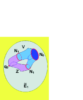
Figure 3. Algebraic singular solution $V^{\prime}=V\bigcup_{N_{1}}Z\subset\tilde{E}_{1}\subset J{\it D}(F)$, passing through a singular point $q_{0}\in A_{3}$.

Note that the symbol $(g_{1})_{q\in A_{3}}=G_{1}\equiv TM\otimes F$, i.e., $(g_{1})_{q\in A_{3}}$ coincides with the symbol of the trivial PDE $J{\it D}(F)\subseteq J{\it D}(F)$. In fact the components of the symbol on $\tilde{E}_{1}$, must satisfy the following equations:

(74) $$\left\{\begin{array}[]{l}Y^{x}_{1}(u^{2}_{y})^{2}+Y^{y}_{2}2u^{1}_{x}u^{2}_{y}=0;\\ \\ Y^{y}_{1}2u^{1}_{y}+Y^{x}_{2}2u^{2}_{x}=0;\\ \\ Y^{x}_{2}u^{3}_{y}+Y^{y}_{3}[u^{2}_{x}+3(u^{3}_{y})^{2}]=0.\\ \end{array}\right\}$$

These equations are identities on $q\in A_{3}$. As a by-product, we get that above considered algebraic singular solutions are, in general, unstable in finite times.

Definition 4.27.

We define extended crystal singular PDE, a singular PDE $E_{k}\subset J^{k}_{n}(W)$ that splits in irreducible components $A_{i}$, i.e., $E_{k}=\bigcup_{i}A_{i}$, where each $A_{i}$ is an extended crystal PDE. Similarly we define extended $0$-crystal singular PDE, (resp. $0$-crystal singular PDE), an extended crystal singular PDE where each component $A_{i}$ is an extended $0$-crystal PDE, (resp. $0$-crystal PDE).

Definition 4.28 (Algebraic singular solutions of singular PDE’s).

Let $E_{k}\subset J^{k}_{n}(W)$ be a singular PDE, that splits in irreducible components $A_{i}$, i.e., $E_{k}=\bigcup_{i}A_{i}$. Then, we say that $E_{k}$ admits an algebraic singular solution $V\subset E_{k}$, if $V\bigcap A_{r}\equiv V_{r}$ is a solution (in the usual sense) in $A_{r}$ for at least two different components $A_{r}$, say $A_{i}$, $A_{j}$, $i\not=j$, and such that one of following conditions are satisfied: (a) ${}_{(ij)}E_{k}\equiv A_{i}\bigcap A_{j}\not=\emptyset$; (b) ${}^{(ij)}E_{k}\equiv A_{i}\bigcup A_{j}$ is a connected set, and ${}_{(ij)}E_{k}=\emptyset$. Then we say that the algebraic singular solution $V$ is in the case (a), weak, singular or smooth, if it is so with respect to the equation ${}_{(ij)}E_{k}$. In the case (b), we can distinguish the following situations: (weak solution): There is a discontinuity in $V$, passing from $V_{i}$ to $V_{j}$; (singular solution): there is not discontinuity in $V$, but the corresponding tangent spaces $TV_{i}$ and $TV_{j}$ do not belong to a same $n$-dimensional Cartan sub-distribution of $J^{k}_{n}(W)$, or alternatively $TV_{i}$ and $TV_{j}$ belong to a same $n$-dimensional Cartan sub-distribution of $J^{k}_{n}(W)$, but the kernel of the canonical projection $(\pi_{k,0})_{*}:TJ^{k}_{n}(W)\to TW$, restricted to $V$ is larger than zero; (smooth solution): there is not discontinuity in $V$ and the tangent spaces $TV_{i}$ and $TV_{j}$ belong to a same $n$-dimensional Cartan sub-distribution of $J^{k}_{n}(W)$ that projects diffeomorphically on $W$ via the canonical projection $(\pi_{k,0})_{*}:TJ^{k}_{n}(W)\to TW$. Then we say that a solution passing through a critical zone bifurcate.

Definition 4.29 (Integral bordism for singular PDE’s).

Let $N_{1},N_{2}\subset E_{k}\subset J^{k}_{n}(W)$ be two $(n-1)$-dimensional admissible closed integral manifolds. We say that $N_{1}$ algebraic integral bords with $N_{2}$, if $N_{1}$ and $N_{2}$ belong to two different irreducible components, say $N_{1}\subset A_{i}$, $N_{2}\subset A_{j}$, $i\not=j$, such that there exists an algebraic singular solution $V\subset E_{k}$ with $\partial V=N_{1}\mathop{\bigcup}\limits^{.}N_{2}$.

In the integral bordism group $\Omega_{n-1}^{E_{k}}$ (resp. $\Omega_{n-1,s}^{E_{k}}$, resp. $\Omega_{n-1,w}^{E_{k}}$) of a singular PDE $E_{k}\subset J^{k}_{n}(W)$, we call algebraic class a class $[N]\in\Omega_{n-1}^{E_{k}}$, (resp. $[N]\in\Omega_{n-1,s}^{E_{k}}$, resp. $[N]\in\Omega_{n-1}^{E_{k}}$,), with $N\subset A_{j}$, such that there exists a closed $(n-1)$-dimensional admissible integral manifolds $X\subset A_{i}\subset E_{k}$, algebraic integral bording with $N$, i.e., there exists a smooth (resp. singular, resp. weak) algebraic singular solution $V\subset E_{k}$, with $\partial V=N\mathop{\bigcup}\limits^{.}X$.

Theorem 4.30 (Singular integral bordism group of singular PDE).

Let $E_{k}\equiv\bigcup_{i}A_{i}\subset J^{k}_{n}(W)$ be a singular PDE. Then under suitable conditions, algebraic singular solutions integrability conditions, we can find (smooth) algebraic singular solutions bording assigned admissible closed smooth $(n-1)$-dimensional integral manifolds $N_{0}$ and $N_{1}$ contained in some component $A_{i}$ and $A_{j}$, $i\not=j$.

Proof.

In fact, we have the following lemmas.

Lemma 4.31.

Let $E_{k}\equiv\bigcup_{i}A_{i}\subset J^{k}_{n}(W)$ be a singular PDE with ${}_{(ij)}E_{k}\equiv A_{i}\bigcap A_{j}\not=\emptyset$. Let us assume that $A_{i}\subset J^{k}_{n}(W)$, $A_{j}\subset J^{k}_{n}(W)$ and ${}_{(ij)}E_{k}\subset J^{k}_{n}(W)$ be formally integrable and completely integrable PDE’s such that $\dim A_{i}>2n+1$, $\dim A_{j}>2n+1$, $\dim{}_{(ij)}E_{k}>2n+1$. Then, one has the following isomorphisms:

(75) $$\Omega_{n-1,w}^{A_{i}}\cong\Omega_{n-1,w}^{A_{j}}\cong\Omega_{n-1,w}^{{}_{(ij)}E_{k}}.$$

So we can find a weak algebraic singular solution $V\subset E_{k}$ such that $\partial V=N_{0}\mathop{\bigcup}\limits^{.}N_{1}$, with $N_{0}\subset A_{i}$, $N_{1}\subset A_{j}$, iff $N_{1}\in[N_{0}]$.

Furthermore, if $g_{k}(A_{i})\not=0$, $g_{k+1}(A_{i})\not=0$, $g_{k}(A_{j})\not=0$, $g_{k+1}(A_{j})\not=0$, $g_{k}({}_{(ij)}E_{k})\not=0$, $g_{k+1}({}_{(ij)}E_{k})\not=0$, then one has also the following isomorphisms:

(76) $$\Omega_{n-1,s}^{A_{i}}\cong\Omega_{n-1,s}^{A_{j}}\cong\Omega_{n-1,s}^{{}_{(ij)}E_{k}}.$$

So we can find a singular algebraic singular solution $V\subset E_{k}$ such that $\partial V=N_{0}\mathop{\bigcup}\limits^{.}N_{1}$, $N_{0}\subset A_{i}$, $N_{1}\subset A_{j}$, iff $N_{1}\in[N_{0}]$.

Proof.

In fact, under the previous hypotheses one has that we can apply Theorem 3.16 to each component $A_{i}$, $A_{j}$ and ${}_{(ij)}E_{k}$ to state that all their weak integral bordism groups of dimension $(n-1)$ are isomorphic to $\bigoplus_{r+s=n-1}H_{r}(W;\mathbb{Z}_{2})\otimes_{\mathbb{Z}_{2}}\Omega_{s}$.

Furthermore, under the above hypotheses on nontriviality of symbols, we can apply Theorem 2.1 in [55]. So we can state that weak integral bordism groups are isomorphic to the corresponding singular ones. ∎

Lemma 4.32.

Let $E_{k}=\bigcup_{i}A_{i}$ be a $0$-crystal singular PDE. Let ${}^{(ij)}E_{k}\equiv A_{i}\bigcup A_{j}$ be connected, and ${}_{(ij)}E_{k}\equiv A_{i}\bigcap A_{j}\not=\emptyset$. Then $\Omega_{n-1,s}^{{}^{(ij)}E_{k}}=0$.

Proof.

In fact, let $Y\subset{}_{(ij)}E_{k}$ be an admissible closed $(n-1)$-dimensional closed integral manifold, then there exists a smooth solution $V_{i}\subset A_{i}$ such that $\partial V_{i}=N_{0}\mathop{\bigcup}\limits^{.}Y$ and a solution $V_{j}\subset A_{j}$ such that $\partial V_{j}=Y\mathop{\bigcup}\limits^{.}N_{1}$. Then, $V=V_{i}\bigcup_{Y}V_{j}$ is an algebraic singular solution of $E_{k}$. This solution is singular in general. ∎

After above lemmas the proof of the theorem can be considered done besides the algebraic singular solutions integrability conditions. ∎

Table 3. Nuclear energy producing magnetohydrodynamics equation $\{\widetilde{F}^{(s)}=0;1\leq s\leq 7\}:\widetilde{(MHD)}\subset J{\it D}^{2}(\widetilde{W})$.

Maxwell	$\widetilde{F}^{(1)}\equiv F^{(1)}\equiv{B^{k}}_{/k}=0$ (no magnetic monopoles)
	$\widetilde{F}^{(2)}\equiv F^{(2)}\equiv{D^{k}}_{/k}-\bar{\rho}4\pi=0$ (Gauss’s law of electrostatic)
	$\widetilde{F}^{(3)}\equiv F^{(3)}{}^{i}\equiv\epsilon^{ijs}E_{j/s}+{{1}\over{c}}(\partial t\cdot B^{i})=0$ (Faraday’s law)
	$\widetilde{F}^{(4)}\equiv F^{(4)}{}^{i}\equiv\epsilon^{ijs}H_{j/s}-{{1}\over{c}}(\partial t\cdot D^{i})-{{4\pi}\over{c}}I^{i}=0$ (Ampere’s law)
	$D^{k}=\epsilon^{ki}E_{i}$, ($\epsilon=$dielectric permeability tensor)
	$\epsilon^{ik}=-\epsilon_{0}g^{ik}+\bar{\epsilon}(v_{r/s}+v_{s/r})g^{ri}g^{sk}$
	$B^{k}=\mu^{ki}H_{i}$, ($\mu=$magnetic permeability tensor)
	$\mu^{ik}=-\mu_{0}g^{ik}+\bar{\mu}(v_{r/s}+v_{s/r})g^{ri}g^{sk}$
Navier-Stokes	$\widetilde{F}^{(5)}\equiv F^{(5)}\equiv{v^{k}}_{/k}=0$ (continuity equation)
	$\widetilde{F}^{(5)}\equiv F^{(5)}_{\alpha}\equiv\dot{x}^{k}(\partial x_{\alpha}.G^{j}_{jk})+\dot{x}^{k}_{\alpha}G^{j}_{jk}+\dot{x}^{s}_{s\alpha}=0$,
	(first-prolonged continuity equation)
	$\widetilde{F}^{(6)}\equiv F^{(6)}{}^{i}\equiv\rho{{\delta v^{i}}\over{\delta t}}-{P^{ik}}_{/k}-F_{(body)}^{i}=0$, (motion equation)
	$\widetilde{F}^{(7)}\equiv\rho C_{v}\frac{\delta\theta}{\delta t}+\frac{\delta w}{\delta t}-\nu(\theta_{/i})_{/k}g^{ik}+S^{k}_{/k}-[2\chi\dot{e}{}^{ik}+\frac{1}{4\pi}(B^{i}B^{k}+E^{i}E^{k})]v_{i/k}$
	$+I^{i}E^{j}g_{ij}-\rho\bar{h}=0$, (energy equation)
	$q^{k}=-\nu\theta_{/i}g^{ik}$, (heat flow)
	$P^{ik}={}^{(rh)}P^{ik}+M^{ik}=-pg^{ik}+\chi(v_{r/s}+v_{s/r})g^{ri}g^{sk}+M^{ik}$
	$\hskip 14.0pt=-g^{ik}[p+\frac{1}{8\pi}(B^{s}B_{s}+E^{s}E_{s})]+\wp^{ik}$ (full stress tensor)
	$\wp^{ki}=\chi(v_{r/s}+v_{s/r})g^{ri}g^{sk}+\frac{1}{4\pi}(B^{i}B^{j}+E^{i}E^{j})$ (deviatory stress)
	(magnetic stress tensor) ${}^{(B)}M^{ij}\equiv\frac{1}{4\pi}(-\frac{1}{2}B^{k}B_{k}g^{ij}+B^{i}B^{j})$
	(electric stress tensor) ${}^{(E)}M^{ij}\equiv\frac{1}{4\pi}(-\frac{1}{2}E^{k}E_{k}g^{ij}+E^{i}E^{j})$
	(e.m. stress tensor) $M^{ij}\equiv{}^{(B)}M^{ij}+{}^{(E)}M^{ij}$.
	(body force): $F_{(body)}^{i}=-\rho(\partial x_{k}.f)g^{ki}+\bar{\rho}E^{i}+\epsilon^{ijk}I_{j}B_{k}$
$\bar{h}$ body energy source density.

Example 4.33 (Extended crystal singular MHD-PDE’s).

In the recent paper [68] we introduced a new PDE of the magnetohydrodynamics encoding the dynamic of anisotropic incompressible plasmas able to describe nuclear energy production. This equation is denoted $\widetilde{(MHD)}\subset J{\it D}^{2}(\widetilde{W})$ and it is reported in Tab. 3. The fiber bundle there considered is $\pi:\widetilde{W}\to M$, over the Galilean space-time $M$, with $\widetilde{W}\equiv M\times\mathbf{I}\times\mathbf{S}^{3}\times\mathbb{R}^{4}$, where $\mathbf{I}$ is an affine $3$-dimensional space (time-like flow velocities space) and $\mathbf{S}$ is a $3$-dimensional Euclidean vector space. A section $s=(v,p,\theta,E,H,I,\bar{\rho},\bar{h})$ represents flow-velocity, isobaric pressure, temperature, electric vector field, magnetic vector field, electric current density, electric charge density, nuclear energy production density. In that paper it is also proved that equation $\widetilde{(MHD)}$ is formally integrable, completely integrable and an extended $0$-crystal. Now, from Theorem 3.16 we can see that for any two space-like admissible Cauchy hypersurfaces $N_{0}\subset\widetilde{(MHD)}_{t_{0}}$, $N_{1}\subset\widetilde{(MHD)}_{t_{1}}$, $t_{1}\not=t_{2}$, there exists a (singular) solution $V\subset\widetilde{(MHD)}$, passing through $N_{0}$ and $N_{1}$. The admissibility requires that $N_{0}$ and $N_{1}$ are smooth $3$-dimensional regular manifolds with respect to the embedding $\widetilde{(MHD)}\subset J^{2}_{4}(\widetilde{W})$, locally satisfying the Cauchy problem and with orientable boundaries $X_{0}\equiv\partial N_{0}$, $X_{1}\equiv\partial N_{1}$, bording by means of a suitable $3$-dimensional time-like integral manifold $P$.

Table 4. Polynomial differential expression for $\theta^{2}\mathcal{R}$.

$\theta^{2}\mathcal{R}=\theta\left[\dot{x}^{a}_{b}\dot{x}^{c}_{d}\mathcal{R}(1)^{bd}_{ac}+\dot{x}^{a}_{b}\dot{x}^{c}_{d}H^{p}H^{q}\mathcal{R}(2)^{bd}_{acpq}+\dot{x}^{a}_{b}\dot{x}^{c}\mathcal{R}(3)^{b}_{ac}+\dot{x}^{a}_{b}\dot{x}^{c}H^{p}H^{q}\mathcal{R}(4)^{b}_{acpq}\right.$

$+\dot{x}^{a}\dot{x}^{b}\mathcal{R}(5)_{ab}+\dot{x}^{a}\dot{x}^{b}\mathcal{R}(6)_{abpq}+\dot{x}^{m}_{s}H^{s}H^{r}\mathcal{R}(7)_{mr}+\dot{x}^{m}_{s}E^{i}E^{j}\mathcal{R}(8)^{s}_{mij}$

$+\dot{x}^{t}H^{q}H^{r}\mathcal{R}(9)_{tqr}+\dot{x}^{t}E^{i}E^{j}\mathcal{R}(10)_{tij}+\dot{x}^{r}_{u}\dot{x}^{a}_{b}\dot{x}^{c}_{d}H^{p}H^{q}\mathcal{R}(11)^{ubd}_{tacpq}+\dot{x}^{r}_{u}\dot{x}^{a}_{b}\dot{x}^{c}H^{p}H^{q}\mathcal{R}(12)^{ub}_{racpq}$

$\left.+\dot{x}^{r}_{u}\dot{x}^{a}\dot{x}^{b}H^{p}H^{q}\mathcal{R}(13)^{u}_{rabpq}+\dot{x}^{w}\dot{x}^{a}\dot{x}^{b}H^{p}H^{q}\mathcal{R}(14)_{wabpq}+\bar{h}\right]+\theta_{j}\theta_{k}\mathcal{R}(15)^{jk}$

$\mathcal{R}(1)^{bd}_{ac}=\frac{\chi}{\rho}(g^{bd}g_{ac}+\delta^{d}_{a}\delta^{b}_{c})$

$\mathcal{R}(2)^{bd}_{acpq}=-\frac{\mu_{0}\bar{\mu}}{4\pi\rho}(\delta^{d}_{a}\delta^{b}_{q}g_{pc}+\delta^{b}_{q}\delta^{d}_{p}g_{ca}+g^{db}g_{qa}g_{pc})$

$\mathcal{R}(3)^{b}_{ac}=\frac{4\chi}{\rho}G^{b}_{ac}$

$\mathcal{R}(4)^{b}_{acpq}=-\frac{\mu_{0}\bar{\mu}}{4\pi\rho}(\delta^{b}_{q}g_{pk}G^{k}_{ac}+\delta^{b}_{q}g_{ka}G^{k}_{pc}+\delta^{b}_{p}g_{aj}G^{j}_{qc}+2g_{pa}G^{b}_{qc}+2g_{aq}G^{b}_{pc}+g_{qt}g_{aj}G^{t}_{kc}G^{k}_{pb})$

$\mathcal{R}(5)_{ab}=\frac{2\chi}{\rho}G^{i}_{sa}G^{s}_{ib}$

$\mathcal{R}(6)_{abpq}=-\frac{\mu_{0}\bar{\mu}}{4\pi\rho}(g_{kj}G^{j}_{qa}G^{k}_{pb}+g_{qt}G^{t}_{ka}G^{k}_{pb}+2g_{pk}G^{j}_{qa}G^{k}_{jb})$

$\mathcal{R}(7)_{mr}=\frac{\mu_{0}^{2}}{4\pi\rho}g_{rm}$

$\mathcal{R}(8)^{s}_{mij}=\frac{1}{8\pi\rho}(\delta^{s}_{j}g_{im}+\delta^{s}_{i}g_{jm})$

$\mathcal{R}(9)_{tqr}=\frac{\mu_{0}}{4\pi\rho}g_{mr}G^{m}_{qt}$

$\mathcal{R}(10)_{tij}=\frac{1}{8\pi\rho}(g_{im}G^{m}_{jt}+g_{jm}G^{m}_{it})$

$\mathcal{R}(11)^{ubd}_{tacpq}=\frac{\bar{\mu}^{2}}{8\pi\rho}(\delta^{d}_{a}\delta^{b}_{q}g_{ic}+\delta^{b}_{q}\delta^{d}_{p}g_{ca}+g^{db}g_{qa}g_{ic})(\delta^{i}_{r}\delta^{u}_{p}+g^{iu}g_{rp})$

$\mathcal{R}(12)^{ub}_{racpq}=\frac{\bar{\mu}^{2}}{4\pi\rho}[\frac{1}{2}(\delta^{b}_{q}g_{ik}G^{k}_{ac}+\delta^{b}_{q}g_{ka}G^{k}_{ic}+\delta^{b}_{i}g_{aj}G^{j}_{qc}+2g_{ia}G^{b}_{qc}+2g_{aq}G^{b}_{ic}+g_{qt}g_{aj}G^{t}_{kc}G^{k}_{ib})$

$(\delta^{i}_{v}\delta^{u}_{p}+g^{iu}g_{rp})$

$\hskip 56.9055pt+(\delta^{u}_{a}\delta^{b}_{q}g_{ir}+\delta^{b}_{q}\delta^{u}_{p}g_{ra}+g^{ab}g_{qa}g_{ir})G^{i}_{pc}]$

$\mathcal{R}(13)^{u}_{rabpq}=\frac{\bar{\mu}^{2}}{4\pi\rho}[\frac{1}{2}(G_{qa}^{j}G_{ib}^{k}g_{kj}+G_{ka}^{t}G_{ib}^{k}g_{qt}+2G_{qa}^{j}G_{jb}^{k}g_{ik})(\delta^{i}_{v}\delta^{u}_{p}+g^{iu}g_{rp})$

$\hskip 56.9055pt+(\delta^{u}_{q}g_{ik}G^{k}_{rb}+\delta^{u}_{q}g_{kr}G^{k}_{ib}+\delta^{u}_{i}g_{rj}G^{j}_{qb}+2g_{ir}G^{u}_{qb}+2g_{rq}G^{k}_{ib}+g_{qt}g_{rj}G^{t}_{kb}G^{k}_{iu})G^{i}_{pa}]$

$\mathcal{R}(14)_{wabpq}=\frac{\bar{\mu}^{2}}{4\pi\rho}(G^{j}_{qa}G^{k}_{ib}g_{kj}+G^{t}_{ka}G^{k}_{ib}g_{qt}+2G^{j}_{qa}G^{k}_{jb}g_{ik}+)G^{i}_{pw}$

$\mathcal{R}(15)^{jk}=\frac{\nu}{\rho}g^{kj}$

Then the solution $V$ has boundary $\partial V=N_{0}\bigcup_{X_{0}}P\bigcup_{X_{1}}N_{1}$. (For details see Refs.[69, 71] There can be also found the explicit expressions of the differential polynomials defining $\widetilde{(MHD)}$.) In [71] we proved that we can identify a sub-equation $\widehat{\underline{(MHD)}}\subset\widetilde{(MHD)}$ such that in some neighborhood of its points, there exist entropy-regular-solutions passing from such initial conditions. More precisely, we can represent $\theta^{2}\mathcal{R}$ as a polynomial differential of first order on $J{\it D}(\widetilde{W})$, belonging to $A[\dot{x}^{a},\dot{x}^{a}_{b},H^{p},E^{p},\theta,\theta_{j},\bar{h}]$, where $A\equiv[[x^{1},x^{2},x^{3}]]$. This can be seen taking into account that

(77) $$\theta^{2}\mathcal{R}(s)=\theta\left[\frac{1}{\rho 4\pi}(B^{i}B^{j}+E^{i}E^{j})\dot{e}_{ij}+\frac{2\chi}{\rho}\dot{e}^{ij}\dot{e}_{ij}+\bar{h}\right]+\frac{\nu}{\rho}(\hbox{\rm grad}\hskip 2.0pt\theta)^{2}.$$

and by calculating the corresponding explicit differential polynomial expression for $\theta^{2}\mathcal{R}:J{\it D}(\widetilde{W})\to\mathbb{R}$. (See Tab. 4.) $\widehat{\underline{(MHD)}}\subset\widetilde{(MHD)}$ is an extended $0$-crystal singular PDE, in the sense of Definition 4.27.

Let us resume the proof given in [71], since this is necessary to understand the further developments reported below. Let us define

(78) $$\underline{(MHD)}\equiv\left\{q\in\widetilde{(MHD)}|\theta(q)>0,\bar{h}(q)\geq 0,\mathcal{R}(q)\geq 0\right\}.$$

Then, $\underline{(MHD)}$ is a connected, simply connected bounded domain in $\widetilde{(MHD)}$. In fact, we can split $\underline{(MHD)}$ in the following way

(79) $$\underline{(MHD)}={}_{(+,+)}\widetilde{Y}_{1}\bigcup{}_{(+,+)}\widetilde{Y}_{2}\bigcup\widetilde{Y}_{3}\bigcup{}_{(+,+,+)}\underline{(MHD)},$$

where

(80) $${}_{(+,+,+)}\underline{(MHD)}\equiv\left\{q\in\widetilde{(MHD)}|\bar{h}(q)>0,\theta(q)>0,\mathcal{R}(q)>0\right\}$$

is an open submanifold of $\widetilde{(MHD)}$, and

(81) $$\left\{\begin{array}[]{ll}{}_{(+,+)}\widetilde{Y}_{1}&\equiv\left\{q\in\widetilde{(MHD)}|\bar{h}(q)=0,\theta(q)>0,\mathcal{R}(q)>0\right\}\\ \\ {}_{(+,+)}\widetilde{Y}_{2}&\equiv\left\{q\in\widetilde{(MHD)}|\mathcal{R}(q)=0,\theta(q)>0,\bar{h}(q)>0\right\}\end{array}\right.$$

are codimension $1$ submanifolds of $\widetilde{(MHD)}$. Furthermore,

(82) $$\widetilde{Y}_{3}\equiv\left\{q\in{}_{(+)}\widetilde{(MHD)}|\bar{h}(q)=0,\mathcal{R}(q)=0\right\}$$

is a codimension $2$ submanifold of

$${}_{(+)}\widetilde{(MHD)}\equiv\left\{q\in\widetilde{(MHD)}|\theta(q)>0\right\}.$$

Let us study the integrability properties of such submanifolds of $\widetilde{(MHD)}$. First note that since ${}_{(+,+,+)}\underline{(MHD)}$ is an open submanifold in $\widetilde{(MHD)}$ and in $J{\it D}^{2}({}_{(+,+)}\widetilde{W})$, where

$${}_{(+,+)}\widetilde{W}\equiv M\times\mathbf{I}\times\mathbb{R}\times\mathbb{R}^{+}\times\mathbf{S}^{3}\times\mathbb{R}\times\mathbb{R}^{+},$$

it follows that if $q\in{}_{(+,+,+)}\underline{(MHD)}$ there exist solutions belonging to ${}_{(+,+,+)}\underline{(MHD)}$, i.e., entropy-regular-solutions passing through $q$, just follows from the fact that ${}_{(+,+,+)}\underline{(MHD)}$ is an open submanifold of $\widetilde{(MHD)}$. So ${}_{(+,+,+)}\underline{(MHD)}$ is completely integrable. Furthermore, since

(83) $$\left\{\begin{array}[]{ll}{}_{(+,+,+)}\underline{(MHD)}_{+r}&=J{\it D}^{r}({}_{(+,+,+)}\underline{(MHD)})\bigcap J{\it D}^{2+r}({}_{(+,+)}\widetilde{W})\\ \\ &\subset J{\it D}^{r}(\widetilde{(MHD)})\bigcap J{\it D}^{2+r}(\widetilde{W})=\widetilde{(MHD)}_{+r}\end{array}\right.$$

it follows that ${}_{(+,+,+)}\underline{(MHD)}$ is also formally integrable. Let us consider the integrability properties of ${}_{(+,+)}\widetilde{Y}_{1}\subset\partial\underline{(MHD)}$. If $q\in{}_{(+,+)}\widetilde{Y}_{1}$ it follows that $q\in{}_{(+)}\widehat{(MHD)}$. Since this last equation is formally integrable and completely integrable, and ${}_{(+,+)}\widetilde{Y}_{1}$ is an open submanifold of ${}_{(+)}\widehat{(MHD)}$, it follows that also ${}_{(+,+)}\widetilde{Y}_{1}$ is formally integrable and completely integrable.

Let us, now, study the integrability properties of

(84) $${}_{(+,+)}\widetilde{Y}_{2}\subset J{\it D}^{2}({}_{(+,+)}\widetilde{W}):\left\{\mathcal{R}=0,\widetilde{F}^{(s)}=0\right\}.$$

One can see that this equation is not formally integrable, but becomes so if we add the first prolongation of $\mathcal{R}=0$. So we can prove that the following equation

(85) $$\widehat{{}_{(+,+)}\widetilde{Y}_{2}}\subset J{\it D}^{2}({}_{(+,+)}\widetilde{W}):\left\{\mathcal{R}=0,\mathcal{R}_{\alpha}=0,\widetilde{F}^{(s)}=0\right\}$$

is formally integrable and completely integrable. Similar considerations can be made on the part $\widetilde{Y}_{3}$, and we can identify, the corresponding formally integrable PDE $\widehat{\widetilde{Y}_{3}}$. We skip on the details. By conclusion we get that

(86) $$\widehat{\underline{(MHD)}}\equiv{}_{(+,+)}\widetilde{Y}_{1}\bigcup\widehat{{}_{(+,+)}\widetilde{Y}_{2}}\bigcup\widehat{\widetilde{Y}_{3}}\bigcup{}_{(+,+,+)}\underline{(MHD)}\subset\widetilde{(MHD)}$$

is the formally integrable and completely integrable constraint in $\widetilde{(MHD)}$, where for any initial condition, passes an entropy-regular-solution for $\widetilde{(MHD)}$. Then we can apply Theorem 3.16 to conclude that $\widehat{\underline{(MHD)}}$ is an extended crystal singular PDE. Furthermore, taking into account that it results

$$\Omega^{\widehat{\underline{(MHD)}}}_{3,w}\cong\Omega^{\widehat{\underline{(MHD)}}}_{3,s}\cong\Omega_{3}=0,$$

we get that $\widehat{\underline{(MHD)}}$ is also an extended $0$-crystal singular PDE. This assures that for any two space-like admissible Cauchy integral manifolds $N_{1}\subset\widehat{\underline{(MHD)}}_{t_{1}}$, $N_{2}\subset\widehat{\underline{(MHD)}}_{t_{2}}$, $t_{1}\not=t_{2}$, such that if both $N_{i}$, $i=1,2$, belong to the same component, in the split given in (86), there exist (singular) entropy-regular-solutions $V$ such that $\partial V=N_{1}\bigcup_{X_{1}}P\bigcup_{X_{2}}N_{2}$, and such that their boundaries $X_{1}\equiv\partial N_{1}$, $X_{2}\equiv\partial N_{2}$, should be orientable and propagating with an admissible $3$-dimensional integral manifold $P$. (For details see [69].) The stability properties of $\widehat{\underline{(MHD)}}$ and its solutions, can be studied by utilizing our recent geometric theory on the stability of PDE’s [67, 68, 69, 70, 71]. More precisely, $\widehat{\underline{(MHD)}}$ is a functionally stable singular PDE, in the sense that it slpits in components that are functionally stable PDE’s. Furthermore, smooth entropy-regular-solutions, i.e., smooth solutions of $\widehat{\underline{(MHD)}}$, do not necessitate to be stable. However, all they can be stabilized and the stable extended crystal singular PDE of $\widehat{\underline{(MHD)}}$, i.e., a singular PDE slpits in components that are stable extended crystal PDE’s. This last is just ${}^{(S)}\widehat{\underline{(MHD)}}=\widehat{\underline{(MHD)}}_{(+\infty)}$. There, all smooth entropy-regular-solutions, belonging to only one of the components, in the split representation (86) are stable at finite times.

Let us, now, find global solutions of $\widehat{\underline{(MHD)}}$, crossing the singular sets corresponding to states without nuclear energy production, to ones where $\bar{h}>0$, i.e., passing from ${}_{(+,+)}\tilde{Y}_{1}$ to ${}_{(+,+,+)}\underline{(MHD)}$. Let $V\subset\widetilde{(MHD)}$ be a time-like solution such that the following conditions are satisfied:

(i) $V$ is a regular entropy solution;

(ii) $V\bigcap{}_{(+,+)}\tilde{Y}_{1}\equiv{}_{(+)}V\not=\emptyset$;

(iii) $V\bigcap{}_{(+,+,+)}\underline{(MHD)}\equiv{}_{(+,+)}V\not=\emptyset$.

(iv) $\partial V=N_{0}\bigcup P\bigcup N_{1}$, $N_{0}\subset{}_{(+)}V$, $N_{1}\subset{}_{(+,+)}V$, $\partial{}_{(+)}V=N_{0}\bigcup{}_{(+)}P\bigcup Y$.

Then we can give the following split surgery representation of $V$:

(87) $$V={}_{(+)}V\bigcup_{Y}Z$$

with $Z=Y\bigcup{}_{(+,+)}V$. We call a solution $V$ of $\widetilde{(MHD)}$, such that holds the surgery property given in (87) just a crossing nuclear critical zone solution. Then, for any two admissible space-like Cauchy hypersurfaces $N_{1}\subset\widehat{\underline{(MHD)}}_{t_{1}}$, $N_{2}\subset\widehat{\underline{(MHD)}}_{t_{2}}$, $t_{1}\not=t_{2}$, such that the following properties are satisfied:

(a) $N_{1}\subset{}_{(+,+)}\tilde{Y}_{1}$;

(b) $N_{2}\subset{}_{(+,+,+)}\underline{(MHD)}$;

there exists a crossing nuclear critical zone solution $V\subset\widetilde{\underline{(MHD)}}$, such that $\partial V=N_{1}\bigcup P\bigcup N_{2}$, where $P$ is a time-like admissible $3$-dimensional integral manifold of $\widetilde{\underline{(MHD)}}$. In general such a solution is a singular solution. Therefore, under above condition of admissibility, one has algebraic classes in $\Omega_{2,s}^{\widehat{\underline{(MHD)}}}$. Furthermore, $V$ is represented by a smooth integral manifold at $Y$, with respect to the split given in (87), if the tangent space $T{}_{(+)}V|_{Y}=TZ|_{Y}\subset\mathbf{E}_{2}\widetilde{(MHD)}|_{Y}$, where $\mathbf{E}_{2}\widetilde{(MHD)}$ is the Cartan distribution of $\widetilde{(MHD)}$. In fact the dimension of the Cartan distribution $\mathbf{E}_{2}$ of $\widehat{\underline{(MHD)}}$ in the points $q\in{}_{(+,+,+)}\underline{(MHD)}$ is higher than in the points $q\in{}_{(+,+)}\tilde{Y}_{1})$. This can be seen by direct computation. Let us denote by

(88) $$\zeta=X^{\alpha}[\partial x_{\alpha}+\sum_{0\leq|\beta|\leq 1}y^{j}_{\alpha\beta}\partial y_{j}^{\beta}]+Z^{j}_{\beta_{1}\beta_{2}}\partial y_{j}^{\beta_{1}\beta_{2}}$$

the generic vector field of the Cartan distribution $\mathbf{E}_{2}(\widetilde{W})$, where

$$\{y^{j}\}_{1\leq j\leq 16}=\{v^{i},p,\theta,E^{i},H^{i},I^{i},\bar{\rho},\bar{h}\}$$

are the vertical coordinates of the fiber bundle $\pi:\widetilde{W}\to M$. The Cartan distribution on the boundary ${}_{(+,+)}\tilde{Y}_{1}\subset\widehat{\underline{(MHD)}}$ is given by the vector fields (88) such that the following equations are satisfied: $\zeta.\bar{F}^{I}=0$, where $\bar{F}^{I}$ are the functions defining equation ${}_{(+,+)}\tilde{Y}_{1}$. These are just the functions defining ${}_{(+,+,+)}\underline{(MHD)}$, i.e., $\widetilde{F}^{(s)}$, $1\leq s\leq 7$, but with the condition $\bar{h}=0$. So we get

(89)

Note that even if the points of ${}_{(+,+)}\tilde{Y}_{1}$ can be considered singular one, with respect to the Cartan distribution of $\widehat{\underline{(MHD)}}$, the embedding $\widehat{\underline{(MHD)}}\subset\widetilde{(MHD)}$ allows us to prolong a solution from ${}_{(+,+)}\tilde{Y}_{1}$ to ${}_{(+,+,+)}\underline{(MHD)}$, according to Theorem 4.30 and surgery representation (87). Then such solution $V$ in general bifurcates along $Y$. By summarizing, we can say that the crossing nuclear critical zone solution $V\subset\widehat{\underline{(MHD)}}$ is represented by an integral manifold $V\subset\widehat{\underline{(MHD)}}$ that is smooth in a neighborhood of $X\subset Y$, iff for its tangent space $TV$, the following condition is satisfied: $T{}_{(+)}V|_{X}=TZ|_{X}\subset\mathbf{E}_{2}(\widetilde{MHD})|_{X}$.

Now, in order to surgery a smooth solution $V^{\prime}\subset{(+,+,+)}\underline{(MHD)}$, passing through a compact smooth space-like $3$-dimensional manifold $N_{1}$, with $X_{1}\equiv\partial N_{1}$ orientable, with suitable smooth solutions of ${}_{(+,+)}\tilde{Y}_{1}$ it is enough that the following conditions should be satisfied:

(90) $$\left\{\begin{array}[]{l}\lim_{\bar{h}\to 0}V^{\prime}={}_{(+,+)}V\subset{{}_{(}+,+,+)}\underline{(MHD)}\\ \\ T{}_{(+,+)}V\subset\mathbf{E}_{2}({(+,+,+)}\underline{(MHD)})_{\bar{h}=0}.\\ \end{array}\right.$$

Since ${}_{(+,+)}V$ is a smooth solution we can prolong it to $\infty$, obtaining a solution ${}_{(+,+)}V^{(\infty)}\subset{}_{(+,+,+)}\underline{(MHD)}_{(+\infty)}$. There it identifies an horizontal $4$-plane $\mathbf{H}\subset\mathbf{E}_{2}({}_{(+,+,+)}\underline{(MHD)}_{(+\infty)})$, contained in the Cartan distribution of ${}_{(+,+,+)}\underline{(MHD)}_{(+\infty)}$. Then $\mathbf{H}$ identifies also an horizontal $4$-plane, that we continue to denote with $\mathbf{H}$, in the Cartan distribution of $\widetilde{(MHD)}_{+\infty}$, that on $({}_{(+,+)}\tilde{Y}_{1})_{+\infty}$, coincides with the Cartan distribution of this last equation. Then we can smoothly prolong ${}_{(+,+)}V^{(\infty)}$ into $({}_{(+,+)}\tilde{Y}_{1})_{+\infty}$, identifying there a smooth solution ${}_{(+)}V^{(\infty)}$. The projection of this algebraic singular solution on ${}_{(+,+)}\tilde{Y}_{1}\bigcup{}_{(+,+,+)}\underline{(MHD)}$ identifies a smooth solution $V$ that has the split surgery property (87). Therefore, it is enough to prove that solutions with the property (90) exist in ${}_{(+,+,+)}\underline{(MHD)}$. Now, we can see that a Cartan vector field $\zeta$ of ${}_{(+,+,+)}\underline{(MHD)}$ is given in (88) and subject to the condition $\zeta.\tilde{F}^{(s)}=0$. Then conditions (90) are satisfied iff $X^{\alpha}{\bar{h}}_{\alpha}=0$. Since this condition can be satisfied for suitable functions $X^{\alpha}$ on ${}_{(+,+,+)}\underline{(MHD)}$, we recognize that in the set of smooth solutions of ${}_{(+,+,+)}\underline{(MHD)}$ exist solutions that smoothly surgery with smooth solutions of ${}_{(+,+)}\tilde{Y}_{1}$. Such solutions are not finite times stable in $\widehat{\underline{(MHD}}$ since there the symbol is not trivial in each components ${}_{(+,+)}\tilde{Y}_{1}$ and ${}_{(+,+,+)}\underline{(MHD)}$. However, by using their formal integrability and complete integrability properties, we can state that in $(\widehat{\underline{(MHD}})_{+\infty}$ such solutions are finite times stable. So $\widehat{\underline{(MHD}})_{+\infty}$ is the stable extended crystal singular PDE associated to $\widehat{\underline{(MHD}}$.

5. APPENDIX A - THE AFFINE CRYSTALLOGRAPHIC GROUP TYPES $[G(3)]$ AND $[G(2)]$

Table 5. The 32 crystallographic point groups of the space-group types $[G(3)]$.

Type Schoenflies Symbol International Symbol nonaxial (2) $C_{i}=S_{2}$, $C_{s}=C_{1h}$ $\bar{1}$, $m$ cyclic (5) $C_{n}$, $n=1,2,3,4,6$ $n$, $n=1,2,3,4,6$ cyclic with horizontal planes (4) $C_{nh}$, $n=2,3,4,6$ $2/m$, $\bar{6}$, $4/m$, $6/m$ cyclic with vertical planes (4) $C_{nv}$, $n=2,3,4,6$ $mm2$, $3m$, $4mm$, $6mm$ dihedral (4) $D_{n}$, $n=2,3,4,6$ $222$, $32$, $422$, $622$ dihedral with horizontal planes (4) $D_{nh}$, $n=2,3,4,6$ $mmm$, $\bar{6}m2$, $4/mmm$, $6/mmm$ dihedral with planes between axes (2) $D_{nd}$, $n=2,3$ $\bar{4}2m$, $\bar{3}m$ improper rotation (2) $S_{n}$, $n=4,6$ $\bar{4}$, $\bar{3}$ cubic groups (5) $T$, $T_{h}$, $T_{d}$, $O$, $O_{h}$ $23$, $m\bar{3}$, $\bar{4}3m$, $432$, $m\bar{3}m$ $n$ ($n=1,2,3,4,6$): rotations of $2\pi/n$ about a symmetry axis. $\bar{n}$ ($n=1,2,3,4,6$): rotation $n$ composed with inversion about symmetry centre; $m=\bar{2}$. $C_{n}=\mathbb{Z}_{n}\cong\{0,1,2,3,\cdots,n-1\}$ (cyclic abelian groups); $C_{i}=S_{2}$; $C_{s}=m$; $C_{3i}=S_{6}$ $D_{n}$: group with an $n$-fold axis plus a two-fold axis perpendicular to that axis. $D_{n}$ is a non abelian group for $n>2$. The group order is $2n$. $D_{nh}$: $D_{n}$ with a mirror plane symmetry perpendicular to the $n$-fold axis. $D_{nv}$: $D_{n}$ with mirror plane symmetries parallel to the $n$-fold axis. $O$: symmetry group of the octahedron. The group order is $24$. One has the isomorphism $O\cong T_{d}$. $O_{h}$: $O$ with improper operations (those that change orientation). The group order is $48$. $T$: symmetry group of the tetrahedron, isomorphic to the alternating group $A_{4}$. The group order is $12$.                  The group order is $12$. $T_{d}$: $\scriptstyle T$ with improper operations. Non abelian group of order $24$. $T_{h}$: $T$ with the addition of an inversion. $A_{n}$: group of even permutations on a set of length $n$. The group order is $\frac{n!}{2}$.

Table 6. Diehdral groups $D_{2m}$, $m\geq 1$.

$m$ $D_{2m}$ $1$ $D_{2}\cong\mathbb{Z}_{2}$ $m\geq 2$ $D_{2m}\cong\mathbb{Z}_{m}\rtimes\mathbb{Z}_{2}$ The generator of $\mathbb{Z}_{2}$ acts on $\mathbb{Z}_{m}$ as multiplication by $-1$ $2$ $D_{4}\cong\mathbb{Z}_{2}\times\mathbb{Z}_{2}$ (Klein four-group) Warn that in crystallography diehdral groups are usually denoted by $D_{m}=D_{2m}$, $m\geq 2$. This is just the notation used in Tab. 5.

Table 7. The 230 affine crystallographic space-group types $[G(3)]$.

Syngonies (7) Geometric classes (32=Point Groups) Bravais types (14) Triclinic $C_{i}=S_{2}(1)$, $C_{1}(1)$ $2P$ Monoclinic $C_{2}(3)$, $C_{1h}(4)$, $C_{2h}(6)$ $8P$, $5C$ Orthorhombic $D_{2}(9)$, $C_{2v}(22)$, $D_{2h}(28)$ $30P$, $15C$, $9I$, $5F$ Tetragonal $C_{4}(6)$, $S_{4}(2)$, $C_{4h}(6)$, $D_{4}(10)$, $C_{4v}(12)$, $D_{2d}(12)$, $D_{4h}(20)$ $49P$, $19I$ Trigonal $C_{6}(4)$, $S_{6}(2)$, $D_{3}(7)$, $C_{3v}(6)$, $D_{3d}(6)$ $18P$, $7R$ Hexagonal $C_{3}(6)$, $C_{3h}(1)$, $C_{6h}(2)$, $D_{6}(6)$, $C_{6v}(4)$, $D_{3h}(4)$, $D_{6h}(4)$ $27P$ Cubic $T(5)$, $T_{h}(7)$, $O(8)$, $T_{d}(6)$, $O_{h}(10)$ $15P$, $11F$, $9I$ (Crystal class systems =Syngonies): 7. (Triclinic=Anorthic), (Trigonal=Rhombohedral). Bravais lattice centering types: $P=$primitive, $I=$body, $F=$face, $A/B/C=$side, $R=$rhombohedral. (For the body-centerd case ($B=I$), the infinite translation group is $\{\mathbb{Z}^{3},\mathbb{Z}^{3}+(\frac{1}{2},\frac{1}{2},\frac{1}{2})\}$.)

Table 8. The 17 affine crystallographic space-group types $[G(2)]$.

Syngony (5) International Symbols Geometric classes (10=Point Groups) Oblique $p1$, $p2$ $\mathbb{Z}_{1}$, $\mathbb{Z}_{2}$ Rectangular $pm$, $pg$, $cm$, $pmm$ $D_{1}$, $D_{1}$, $D_{1}$, $D_{2}$ Rhombic $pmg$, $pgg$, $cmm$ $D_{2}$, $D_{2}$, $D_{2}$ Square $p4$, $p4m$, $p4g$ $\mathbb{Z}_{4}$, $D_{4}$, $D_{4}$ Trigonal $p3$, $p3m1$, $p31m$ $\mathbb{Z}_{3}$, $D_{3}$, $D_{3}$ Hexagonal $p6$, $p6m$ $\mathbb{Z}_{6}$, $D_{6}$ All planar crystallographic groups $G(2)$ are subgroups of $p4m$ or $p6m$, or both. (See Appendix D.) $p=$primitive, $c=$centered, $m=$mirror plane, $g=$glide reflection. A glide reflection is an isometry of the Euclidean plane that combines reflection in a line with a translation along that line.

Table 9. The 4 holohedries (lattice symmetries) in $[G(2)]$.

Holohedry Lattice system $2$ monoclinic=oblique $2mm$ orthorohmbic=$\{$rectangular,rhombic$\}$ $4mm$ tetragonal=square $6mm$ hexagonal=$\{$trigonal,hexagonal$\}$

Table 10. The 7 holohedries (lattice symmetries) in $[G(3)]$.

Holohedry Lattice system $\bar{1}$ triclinic $2/m$ monoclinic $mmm$ orthorohmbic $4/mmm$ tetragonal (square) $\bar{3}m$ trigonal (rombohedric) $6/mmm$ hexagonal $m\bar{3}m$ cubic

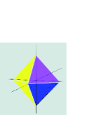
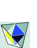
Figure 4. Octahedron and Tetrahedron $3$-chains in $\mathbb{R}^{3}$. (The tetrahedron is a $3$-chain in $\mathbb{R}^{3}$, identified with a regular $4$-faced polyhedron, where each face is an equilateral triangle. It can be derived from the octahedron by extending alternate faces until they meet.)

6. APPENDIX B - THE SUBGROUPS OF THE AFFINE CRYSTALLOGRAPHIC POINT-GROUP TYPES $[G(3)]$

$\scriptstyle C_{i}=S_{2}$ Subgroup Order Index $\scriptstyle-1$ $\scriptstyle 2$ $\scriptstyle 1$ $\scriptstyle 1$ $\scriptstyle 1$ $\scriptstyle 2$ $\scriptstyle C_{s}=C_{1h}$ Subgroup Order Index $\scriptstyle m$ $\scriptstyle 2$ $\scriptstyle 1$ $\scriptstyle 1$ $\scriptstyle 1$ $\scriptstyle 2$ $\scriptstyle C_{1}$ Subgroup Order Index $\scriptstyle 1$ $\scriptstyle 1$ $\scriptstyle 1$

$\scriptstyle C_{2}$ Subgroup Order Index $\scriptstyle 2$ $\scriptstyle 2$ $\scriptstyle 1$ $\scriptstyle 1$ $\scriptstyle 1$ $\scriptstyle 2$ $\scriptstyle C_{3}$ Subgroup Order Index $\scriptstyle 3$ $\scriptstyle 3$ $\scriptstyle 1$ $\scriptstyle 2$ $\scriptstyle 2$ $\scriptstyle 3$ $\scriptstyle C_{4}$ Subgroup Order Index $\scriptstyle 4$ $\scriptstyle 4$ $\scriptstyle 1$ $\scriptstyle 2$ $\scriptstyle 2$ $\scriptstyle 2$ $\scriptstyle 1$ $\scriptstyle 1$ $\scriptstyle 4$

$\scriptstyle C_{6}$ Subgroup Order Index $\scriptstyle 6$ $\scriptstyle 6$ $\scriptstyle 1$ $\scriptstyle 3$ $\scriptstyle 3$ $\scriptstyle 2$ $\scriptstyle 2$ $\scriptstyle 2$ $\scriptstyle 3$ $\scriptstyle 1$ $\scriptstyle 1$ $\scriptstyle 6$ $\scriptstyle C_{2h}$ Subgroup Order Index $\scriptstyle 2/m$ $\scriptstyle 4$ $\scriptstyle 1$ $\scriptstyle 2$ $\scriptstyle 2$ $\scriptstyle 2$ $\scriptstyle m$ $\scriptstyle 2$ $\scriptstyle 2$ $\scriptstyle-1$ $\scriptstyle 2$ $\scriptstyle 2$ $\scriptstyle 1$ $\scriptstyle 1$ $\scriptstyle 4$ $\scriptstyle C_{3h}$ Subgroup Order Index $\scriptstyle-6$ $\scriptstyle 6$ $\scriptstyle 1$ $\scriptstyle 3$ $\scriptstyle 3$ $\scriptstyle 2$ $\scriptstyle m$ $\scriptstyle 2$ $\scriptstyle 3$ $\scriptstyle 1$ $\scriptstyle 1$ $\scriptstyle 6$

$\scriptstyle C_{4h}$ Subgroup Order Index $\scriptstyle 4/m$ $\scriptstyle 8$ $\scriptstyle 1$ $\scriptstyle 4$ $\scriptstyle 4$ $\scriptstyle 2$ $\scriptstyle-4$ $\scriptstyle 4$ $\scriptstyle 2$ $\scriptstyle 2/m$ $\scriptstyle 4$ $\scriptstyle 2$ $\scriptstyle 2$ $\scriptstyle 2$ $\scriptstyle 4$ $\scriptstyle m$ $\scriptstyle 2$ $\scriptstyle 4$ $\scriptstyle-1$ $\scriptstyle 2$ $\scriptstyle 4$ $\scriptstyle 1$ $\scriptstyle 1$ $\scriptstyle 8$ $\scriptstyle C_{6h}$ Subgroup Order Index $\scriptstyle 6/m$ $\scriptstyle 12$ $\scriptstyle 1$ $\scriptstyle-6$ $\scriptstyle 6$ $\scriptstyle 2$ $\scriptstyle 6$ $\scriptstyle 6$ $\scriptstyle 2$ $\scriptstyle-3$ $\scriptstyle 6$ $\scriptstyle 2$ $\scriptstyle 3$ $\scriptstyle 3$ $\scriptstyle 4$ $\scriptstyle 2/m$ $\scriptstyle 4$ $\scriptstyle 3$ $\scriptstyle m$ $\scriptstyle 2$ $\scriptstyle 6$ $\scriptstyle-1$ $\scriptstyle 2$ $\scriptstyle 6$ $\scriptstyle 1$ $\scriptstyle 1$ $\scriptstyle 12$ $\scriptstyle C_{2v}$ Subgroup Order Index $\scriptstyle mm2$ $\scriptstyle 4$ $\scriptstyle 1$ $\scriptstyle 2$ $\scriptstyle 2$ $\scriptstyle 2$ $\scriptstyle m$ $\scriptstyle 2$ $\scriptstyle 2$ $\scriptstyle 1$ $\scriptstyle 1$ $\scriptstyle 4$

$\scriptstyle C_{3v}$ Subgroup Order Index $\scriptstyle 3m$ $\scriptstyle 6$ $\scriptstyle 1$ $\scriptstyle m$ $\scriptstyle 2$ $\scriptstyle 3$ $\scriptstyle 1$ $\scriptstyle 1$ $\scriptstyle 6$ $\scriptstyle C_{4v}$ Subgroup Order Index $\scriptstyle 4mm$ $\scriptstyle 8$ $\scriptstyle 1$ $\scriptstyle 4$ $\scriptstyle 4$ $\scriptstyle 2$ $\scriptstyle mm2$ $\scriptstyle 4$ $\scriptstyle 2$ $\scriptstyle 2$ $\scriptstyle 2$ $\scriptstyle 4$ $\scriptstyle m$ $\scriptstyle 2$ $\scriptstyle 4$ $\scriptstyle 1$ $\scriptstyle 1$ $\scriptstyle 8$ $\scriptstyle C_{6v}$ Subgroup Order Index $\scriptstyle 6mm$ $\scriptstyle 12$ $\scriptstyle 1$ $\scriptstyle 6$ $\scriptstyle 6$ $\scriptstyle 2$ $\scriptstyle 3m$ $\scriptstyle 6$ $\scriptstyle 2$ $\scriptstyle mm2$ $\scriptstyle 4$ $\scriptstyle 3$ $\scriptstyle 2$ $\scriptstyle 2$ $\scriptstyle 6$ $\scriptstyle m$ $\scriptstyle 2$ $\scriptstyle 6$ $\scriptstyle 1$ $\scriptstyle 1$ $\scriptstyle 12$

$\scriptstyle D_{2}$ Subgroup Order Index $\scriptstyle 222$ $\scriptstyle 4$ $\scriptstyle 1$ $\scriptstyle 2$ $\scriptstyle 2$ $\scriptstyle 2$ $\scriptstyle 1$ $\scriptstyle 1$ $\scriptstyle 4$ $\scriptstyle D_{3}$ Subgroup Order Index $\scriptstyle 32$ $\scriptstyle 6$ $\scriptstyle 1$ $\scriptstyle 3$ $\scriptstyle 3$ $\scriptstyle 2$ $\scriptstyle 2$ $\scriptstyle 2$ $\scriptstyle 3$ $\scriptstyle 1$ $\scriptstyle 1$ $\scriptstyle 6$ $\scriptstyle D_{4}$ Subgroup Order Index $\scriptstyle 422$ $\scriptstyle 8$ $\scriptstyle 1$ $\scriptstyle 4$ $\scriptstyle 4$ $\scriptstyle 2$ $\scriptstyle 222$ $\scriptstyle 4$ $\scriptstyle 2$ $\scriptstyle 2$ $\scriptstyle 2$ $\scriptstyle 4$ $\scriptstyle 1$ $\scriptstyle 1$ $\scriptstyle 8$

$\scriptstyle D_{6}$ Subgroup Order Index $\scriptstyle 622$ $\scriptstyle 12$ $\scriptstyle 1$ $\scriptstyle 6$ $\scriptstyle 6$ $\scriptstyle 2$ $\scriptstyle 32$ $\scriptstyle 6$ $\scriptstyle 1$ $\scriptstyle 3$ $\scriptstyle 3$ $\scriptstyle 4$ $\scriptstyle 2$ $\scriptstyle 2$ $\scriptstyle 6$ $\scriptstyle m$ $\scriptstyle 2$ $\scriptstyle 6$ $\scriptstyle 1$ $\scriptstyle 1$ $\scriptstyle 12$ $\scriptstyle D_{2h}$ Subgroup Order Index $\scriptstyle mmm$ $\scriptstyle 8$ $\scriptstyle 1$ $\scriptstyle mm2$ $\scriptstyle 4$ $\scriptstyle 2$ $\scriptstyle 222$ $\scriptstyle 4$ $\scriptstyle 2$ $\scriptstyle 2/m$ $\scriptstyle 4$ $\scriptstyle 2$ $\scriptstyle 2$ $\scriptstyle 2$ $\scriptstyle 4$ $\scriptstyle m$ $\scriptstyle 2$ $\scriptstyle 4$ $\scriptstyle-1$ $\scriptstyle 2$ $\scriptstyle 4$ $\scriptstyle 1$ $\scriptstyle 1$ $\scriptstyle 8$ $\scriptstyle D_{3h}$ Subgroup Order Index $\scriptstyle-6$ $\scriptstyle 6$ $\scriptstyle 1$ $\scriptstyle 3$ $\scriptstyle 3$ $\scriptstyle 2$ $\scriptstyle m$ $\scriptstyle 2$ $\scriptstyle 3$ $\scriptstyle 1$ $\scriptstyle 1$ $\scriptstyle 6$

$\scriptstyle D_{4h}$ Subgroup Order Index $\scriptstyle 4/mmm$ $\scriptstyle 16$ $\scriptstyle 1$ $\scriptstyle-42m$ $\scriptstyle 8$ $\scriptstyle 2$ $\scriptstyle 422$ $\scriptstyle 8$ $\scriptstyle 2$ $\scriptstyle 4/m$ $\scriptstyle 8$ $\scriptstyle 2$ $\scriptstyle 4$ $\scriptstyle 4$ $\scriptstyle 4$ $\scriptstyle-4$ $\scriptstyle 4$ $\scriptstyle 4$ $\scriptstyle mmm$ $\scriptstyle 8$ $\scriptstyle 2$ $\scriptstyle mm2$ $\scriptstyle 4$ $\scriptstyle 4$ $\scriptstyle 222$ $\scriptstyle 4$ $\scriptstyle 4$ $\scriptstyle 2/m$ $\scriptstyle 4$ $\scriptstyle 4$ $\scriptstyle m$ $\scriptstyle 2$ $\scriptstyle 8$ $\scriptstyle 2$ $\scriptstyle 2$ $\scriptstyle 8$ $\scriptstyle-1$ $\scriptstyle 2$ $\scriptstyle 8$ $\scriptstyle 1$ $\scriptstyle 1$ $\scriptstyle 16$ $\scriptstyle D_{6h}$ Subgroup Order Index $\scriptstyle 6/mm$ $\scriptstyle 24$ $\scriptstyle 1$ $\scriptstyle-62m$ $\scriptstyle 12$ $\scriptstyle 2$ $\scriptstyle 6mm$ $\scriptstyle 12$ $\scriptstyle 2$ $\scriptstyle 622$ $\scriptstyle 12$ $\scriptstyle 2$ $\scriptstyle 6/m$ $\scriptstyle 12$ $\scriptstyle 2$ $\scriptstyle-3m$ $\scriptstyle 12$ $\scriptstyle 2$ $\scriptstyle-6$ $\scriptstyle 6$ $\scriptstyle 4$ $\scriptstyle 6$ $\scriptstyle 6$ $\scriptstyle 4$ $\scriptstyle 3m$ $\scriptstyle 6$ $\scriptstyle 4$ $\scriptstyle 32$ $\scriptstyle 6$ $\scriptstyle 4$ $\scriptstyle-3$ $\scriptstyle 6$ $\scriptstyle 4$ $\scriptstyle 6/m$ $\scriptstyle 12$ $\scriptstyle 2$ $\scriptstyle 3$ $\scriptstyle 3$ $\scriptstyle 8$ $\scriptstyle mmm$ $\scriptstyle 8$ $\scriptstyle 3$ $\scriptstyle mm2$ $\scriptstyle 4$ $\scriptstyle 6$ $\scriptstyle 222$ $\scriptstyle 4$ $\scriptstyle 6$ $\scriptstyle 2/m$ $\scriptstyle 4$ $\scriptstyle 6$ $\scriptstyle 2$ $\scriptstyle 2$ $\scriptstyle 12$ $\scriptstyle m$ $\scriptstyle 2$ $\scriptstyle 12$ $\scriptstyle-1$ $\scriptstyle 2$ $\scriptstyle 12$ $\scriptstyle 1$ $\scriptstyle 1$ $\scriptstyle 24$ $\scriptstyle D_{2d}$ Subgroup Order Index $\scriptstyle-42m$ $\scriptstyle 8$ $\scriptstyle 1$ $\scriptstyle-4$ $\scriptstyle 4$ $\scriptstyle 2$ $\scriptstyle mm2$ $\scriptstyle 4$ $\scriptstyle 2$ $\scriptstyle 222$ $\scriptstyle 4$ $\scriptstyle 2$ $\scriptstyle 2$ $\scriptstyle 2$ $\scriptstyle 4$ $\scriptstyle m$ $\scriptstyle 2$ $\scriptstyle 4$ $\scriptstyle 1$ $\scriptstyle 1$ $\scriptstyle 8$

$\scriptstyle D_{3d}$ Subgroup Order Index $\scriptstyle-3m$ $\scriptstyle 12$ $\scriptstyle 1$ $\scriptstyle 3m$ $\scriptstyle 6$ $\scriptstyle 2$ $\scriptstyle 32$ $\scriptstyle 6$ $\scriptstyle 2$ $\scriptstyle-3$ $\scriptstyle 6$ $\scriptstyle 2$ $\scriptstyle 3$ $\scriptstyle 3$ $\scriptstyle 4$ $\scriptstyle 2/m$ $\scriptstyle 4$ $\scriptstyle 3$ $\scriptstyle m$ $\scriptstyle 2$ $\scriptstyle 6$ $\scriptstyle-1$ $\scriptstyle 2$ $\scriptstyle 6$ $\scriptstyle 1$ $\scriptstyle 1$ $\scriptstyle 12$ $\scriptstyle S_{4}$ Subgroup Order Index $\scriptstyle-4$ $\scriptstyle 4$ $\scriptstyle 1$ $\scriptstyle 2$ $\scriptstyle 2$ $\scriptstyle 2$ $\scriptstyle 1$ $\scriptstyle 1$ $\scriptstyle 4$ $\scriptstyle S_{6}=C_{3i}$ Subgroup Order Index $\scriptstyle-3$ $\scriptstyle 6$ $\scriptstyle 1$ $\scriptstyle 3$ $\scriptstyle 3$ $\scriptstyle 2$ $\scriptstyle-1$ $\scriptstyle 2$ $\scriptstyle 3$ $\scriptstyle 1$ $\scriptstyle 1$ $\scriptstyle 6$

$\scriptstyle T$ Subgroup Order Index $\scriptstyle 23$ $\scriptstyle 12$ $\scriptstyle 1$ $\scriptstyle 3$ $\scriptstyle 3$ $\scriptstyle 4$ $\scriptstyle 222$ $\scriptstyle 4$ $\scriptstyle 3$ $\scriptstyle 2$ $\scriptstyle 2$ $\scriptstyle 6$ $\scriptstyle 1$ $\scriptstyle 1$ $\scriptstyle 12$ $\scriptstyle T_{h}$ Subgroup Order Index $\scriptstyle m-3$ $\scriptstyle 24$ $\scriptstyle 1$ $\scriptstyle 23$ $\scriptstyle 12$ $\scriptstyle 2$ $\scriptstyle-3$ $\scriptstyle 6$ $\scriptstyle 4$ $\scriptstyle 3$ $\scriptstyle 3$ $\scriptstyle 8$ $\scriptstyle mmm$ $\scriptstyle 8$ $\scriptstyle 3$ $\scriptstyle mm2$ $\scriptstyle 4$ $\scriptstyle 6$ $\scriptstyle 222$ $\scriptstyle 4$ $\scriptstyle 6$ $\scriptstyle 2/m$ $\scriptstyle 4$ $\scriptstyle 6$ $\scriptstyle 2$ $\scriptstyle 2$ $\scriptstyle 12$ $\scriptstyle m$ $\scriptstyle 2$ $\scriptstyle 12$ $\scriptstyle-1$ $\scriptstyle 2$ $\scriptstyle 12$ $\scriptstyle 1$ $\scriptstyle 1$ $\scriptstyle 24$ $\scriptstyle T_{d}$ Subgroup Order Index $\scriptstyle-43m$ $\scriptstyle 24$ $\scriptstyle 1$ $\scriptstyle 23$ $\scriptstyle 12$ $\scriptstyle 2$ $\scriptstyle 3m$ $\scriptstyle 6$ $\scriptstyle 4$ $\scriptstyle 3$ $\scriptstyle 3$ $\scriptstyle 8$ $\scriptstyle-42m$ $\scriptstyle 8$ $\scriptstyle 3$ $\scriptstyle-4$ $\scriptstyle 4$ $\scriptstyle 6$ $\scriptstyle mm2$ $\scriptstyle 4$ $\scriptstyle 6$ $\scriptstyle 222$ $\scriptstyle 4$ $\scriptstyle 6$ $\scriptstyle 2$ $\scriptstyle 2$ $\scriptstyle 12$ $\scriptstyle m$ $\scriptstyle 2$ $\scriptstyle 12$ $\scriptstyle 1$ $\scriptstyle 1$ $\scriptstyle 24$

$\scriptstyle O$ Subgroup Order Index $\scriptstyle 432$ $\scriptstyle 24$ $\scriptstyle 1$ $\scriptstyle 23$ $\scriptstyle 12$ $\scriptstyle 2$ $\scriptstyle 32$ $\scriptstyle 6$ $\scriptstyle 4$ $\scriptstyle 422$ $\scriptstyle 8$ $\scriptstyle 3$ $\scriptstyle 4$ $\scriptstyle 4$ $\scriptstyle 6$ $\scriptstyle 3$ $\scriptstyle 3$ $\scriptstyle 8$ $\scriptstyle 222$ $\scriptstyle 4$ $\scriptstyle 6$ $\scriptstyle 2$ $\scriptstyle 2$ $\scriptstyle 12$ $\scriptstyle 1$ $\scriptstyle 1$ $\scriptstyle 24$ $\scriptstyle O_{h}$ Subgroup Order Index $\scriptstyle m-3m$ $\scriptstyle 48$ $\scriptstyle 1$ $\scriptstyle-43m$ $\scriptstyle 24$ $\scriptstyle 2$ $\scriptstyle 432$ $\scriptstyle 24$ $\scriptstyle 2$ $\scriptstyle m-3$ $\scriptstyle 24$ $\scriptstyle 2$ $\scriptstyle 23$ $\scriptstyle 12$ $\scriptstyle 4$ $\scriptstyle-3m$ $\scriptstyle 12$ $\scriptstyle 4$ $\scriptstyle 3m$ $\scriptstyle 6$ $\scriptstyle 8$ $\scriptstyle 32$ $\scriptstyle 6$ $\scriptstyle 8$ $\scriptstyle-3$ $\scriptstyle 6$ $\scriptstyle 8$ $\scriptstyle 3$ $\scriptstyle 3$ $\scriptstyle 16$ $\scriptstyle 4/mmm$ $\scriptstyle 16$ $\scriptstyle 3$ $\scriptstyle-42m$ $\scriptstyle 8$ $\scriptstyle 6$ $\scriptstyle 4mm$ $\scriptstyle 8$ $\scriptstyle 6$ $\scriptstyle 422$ $\scriptstyle 8$ $\scriptstyle 6$ $\scriptstyle 4/m$ $\scriptstyle 8$ $\scriptstyle 6$ $\scriptstyle-4$ $\scriptstyle 4$ $\scriptstyle 12$ $\scriptstyle 4$ $\scriptstyle 4$ $\scriptstyle 12$ $\scriptstyle mmm$ $\scriptstyle 8$ $\scriptstyle 6$ $\scriptstyle 222$ $\scriptstyle 4$ $\scriptstyle 12$ $\scriptstyle 2/m$ $\scriptstyle 4$ $\scriptstyle 12$ $\scriptstyle 2$ $\scriptstyle 2$ $\scriptstyle 24$ $\scriptstyle m$ $\scriptstyle 2$ $\scriptstyle 24$ $\scriptstyle-1$ $\scriptstyle 2$ $\scriptstyle 24$ $\scriptstyle 1$ $\scriptstyle 1$ $\scriptstyle 48$

7. APPENDIX C - AMALGAMATED FREE PRODUCTS IN THE AFFINE CRYSTALLOGRAPHIC SPACE-GROUP TYPES $[G(3)]$

Amalgamated free products in $$\scriptstyle[G(3)]$$

reflection over -axis; reflection over -axis.

8. APPENDIX D - THE SUBGROUPS OF THE AFFINE CRYSTALLOGRAPHIC SPACE-GROUP TYPES $[G(2)]$

$$\scriptstyle p2$$

Subgroup Index

Subgroup Index

Subgroup Index

$$\scriptstyle cm$$

Subgroup Index

Subgroup Index

Subgroup Index

$$\scriptstyle p4$$

Subgroup Index

Subgroup Index

Subgroup Index

$$\scriptstyle p4g$$

Subgroup Index

Subgroup Index

Subgroup Index

$$\scriptstyle p3m1$$

Subgroup Index

Subgroup Index

Subgroup Index

References

- [1] H. Abels, Discrete groups of affine isometries, J. Lie Theory 9(1999), 321–349.
- [2] R. P. Agarwal and A. Prástaro, Geometry of PDE’s.III(I): Webs on PDE’s and integral bordism groups. The general theory, Adv. Math. Sci. Appl. 17(1)(2007), 239–266; Geometry of PDE’s.III(II): Webs on PDE’s and integral bordism groups. Applications to Riemannian geometry PDE’s, Adv. Math. Sci. Appl. 17(1)(2007), 267–281.
- [3] R. P. Agarwal and A. Prástaro, Singular PDE’s geometry and boundary value problems, J. Nonlinear Conv. Anal. 9(3)(2008), 417–460; On singular PDE’s geometry and boundary value problems, Appl. Anal. 88(8)(2009), 1115–1131.
- [4] J. L. Alperin and R. B. Bell, Groups and Representations, Gradueate Text in Mathematics 162, Springer, 1995.
- [5] M.T. Anderson, Geometrization of -manifolds via the Ricci flow, Notices Amer. Math. Soc. 51 (2004), 184 193.
- [6] G. Arfken, Crystallographic Point and Space Groups, Mathematical Methods for Physicists, 3rd ed. Orlando, FL., Academic Press, 1985.
- [7] J. Bernstein and O. Schwarzman, Complex crystallographic Coxeter groups and affine root systems, J. Nonlinear Math. Phys. 13(2)(2006), 163–182; Chevally’s theorem for the complex crystallographic groups, J. Nonlinear Math. Phys. 13(3)(2006), 323–351.
- [8] L. Bieberbach, Über die bewegungsgruppen der Euklidschen räume.I, Math. Ann. 70(1911), 297–336; II., Math. Ann. 72(1912), 400–412.
- [9] J. M. Boardman, Singularities of differentiable maps, Publ. Math. Inst. Hautes Études Sci. 33(1967), 21–57.
- [10] N. Bourbaki, Lie Groups and Lie Algebras, Chapters 4-6, Springer-Verlag, Berlin, 2002; Lie Groups and Lie Algebras, Chapters 7-9, Springer-Verlag, Berlin, 2005.
- [11] K. S. Brown, Cohomology of Groups, Springer-Verlag, Paris 1969.
- [12] R. L. Bryant, S. S. Chern, R. B. Gardner, H. L. Goldschmidt & P. A. Griffiths, (1991), Exterior differential systems, Springer-Verlag, New York.
- [13] S. Buoncristiano, C. P. Rourke and B. J. Sanderson, A Geometric Approach to Homology Theory, London Math. Soc. Lecture Note Ser. 18, Cambridge Univ. Press, Cambridge, 1976. Springer-Verlag, New York.
- [14] S. Cappel, A. Ranicki and J. Rosenberg (eds.), (1999), Surveys on Surgery Theory: Volume 1, Papers dedicated to C. T. C. Wall, Princeton University Press, Princeton, New Jersey.
- [15] L. S. Charlap, Bieberbach Groups and Flat Manifolds, Springer-Verlag, New York, 1986.
- [16] B. Chow, S-C. Chu, D. Gliekenstein, C. Guenther, J. Isenberg, T. Ivey, D. Knopf, P. Lu, F. Luo and L. Ni, The Ricci Flow: Techniques and Applications: Part I: Geometric Aspects, Mathematical Surveys Monographs 135, Amer. Math. Soc. 2008.
- [17] B. Chow, S-C. Chu, D. Gliekenstein, C. Guenther, J. Isenberg, T. Ivey, D. Knopf, P. Lu, F. Luo and L. Ni, The Ricci Flow: Techniques and Applications: Part II: Analytic Aspects, Mathematical Surveys Monographs 144, Amer. Math. Soc. 2008.
- [18] B. Chow and D. Knopp, The Ricci flow: an introduction, Mathematical Surveys and Monographs, vol. 110, Amer. Math. Soc. 2004.
- [19] D. M. De Turk, Deforming metrics in the direction of their Ricci tensors, J. Differential Geom. 18(1)(1983), 157–162.
- [20] K. J. Falconer, Fractal Geometry. Mathematical Foundations and Applications. 2nd Revised edition, J. Wiley & Sons Ltd, 2003.
- [21] E. S. Fedorov, The Symmetry and Structure of Crystals. Fundamenta Works., Moscow (1949), 111-255. (In Russian).
- [22] H. Goldshmidt, Integrability criteria for systems of non-linear partial differential equations, J. Differential Geom. 1(1967), 269–307.
- [23] H. Goldshmidt and D. Spencer, Submanifolds and over-determined differential operators, Complex Analysis & Algebraic Geometry, Cambridge, 1977, 319–356.
- [24] M. Golubitsky and V. Guillemin, Stable Mappings and Their Singularities, Springer-Verlag, New York, 1973.
- [25] M. Gromov (1986), Almost flat manifolds, J. Differential Geom. 13(1978), 231–241; Almost Flat Manifolds, Astérisque 81, Soc. Math. France, Paris, 1981.
- [26] R. S. Hamilton, Three-manifolds with positive Ricci curvature, J. Differential. Geom. 17(1982), 255–306.
- [27] R. S. Hamilton, Four-manifolds with positive Ricci curvature operator, J. Differential Geom. 24(1986), 153–179.
- [28] R. S. Hamilton, Eternal solutions to the Ricci flow, J. Differential Geom. 38(1993), 1–11.
- [29] R. S. Hamilton, The formation of singularities in the Ricci flow, Surveys in Differential Geometry 2, International Press, 1995, pp. 7–136.
- [30] R. S. Hamilton, A compactness property for solutions of the Ricci flow on three-manifolds, Comm. Anal. Geom. 7(1999), 695–729.
- [31] M. W. Hirsh, Differential Topology, Springer-Verlag, Berlin 1976.
- [32] S. Kobayashi and K. Nomizu, Foundations of Differential Geometry, vol. I, II, Interscience Publishers, John Wiley & Sons, Inc., New York, 1966. Reprint 1996.
- [33] I. S. Krasilśhchik, V. Lychagin and A. M. Vinogradov, Geometry of Jet Spaces and Nonlinear Partial Differential Equations, Gordon and Breach Science Publishers S.A., Amsterdam 1986.
- [34] M. Kuranishi, On the Cartan prolongation theorem of exsterior differential systems, Amer. J. Math. 79(1)(1957), 1–47.
- [35] M. L. Lapidus and M. van Frankenhuijsen, Fractal Geoemetry and Applications. A Jubilee of Benoit Mandelbrot, Proceedings of Simposia in Purew Math. 72, Amer. Math. Soc., 2005.
- [36] P. L. Lions and M. Crandall, Viscosity solutions of Hamilton-Jacobi equations, Trans. Amer. Math. Soc. 277(1983), 1–42.
- [37] A. M. Ljapunov, Stability of Motion, with an contribution by V. A. Pliss and an introduction by V. P. Basov. Mathematics in Science and Engineering, 30, Academic Press, New York-London, 1966.
- [38] V. Lychagin and A. Prástaro, Singularities of Cauchy data, characteristics, cocharacteristics and integral cobordism, Differential Geom. Appl. 4(1994), 287–300.
- [39] I. B. Madsen and R. J. Milgram, The Classifying Spaces for Surgery and Bordism of Manifolds, Ann. Math. Studies 92, Princeton Univ. Press, NJ, 1979.
- [40] B. B. Mandelbrot, The Fractal Geometry of Nature, W. H. Freeman Co., New York, 1982.
- [41] J. Milnor and J. Stasheff, Characteristic Classes, Ann. Math. Studies 76, Princeton Univ. Press, 1974.
- [42] J. Morgan and D. Sullivan, The transversality characteristic class and linking sycles in surgery theory, Ann. of Math. 99(1974), 463–544.
- [43] G. Perelman, The entropy formula for the Ricci flow and its geometry applications, arXiv:math/0211159.
- [44] G. Perelman, Ricci flow with surgery on three-manifolds, arXiv:math/0303109.
- [45] W. Plesken and M. Pest, On maximal finite irreducible subgroup of , I, II, Math. Computation 31 (1977), 536–551; 552–573.
- [46] A. Prástaro, Dynamic conservation laws, Geometrodynamics Proceedings 1985, A. Prástaro (ed.), World Scientific Publishing Co., Singapore
- [47] A. Prástaro, Cobordism of PDE’s, Boll. Unione Mat. Ital. 30(5-B)(1991), 977–1001.
- [48] A. Prástaro, Quantum geometry of PDE’s, Rep. Math. Phys. 30(3)(1991), 273–354.
- [49] A. Prástaro, Geometry of super PDE’s, Geometry in Partial Differential Equations, A. Prástaro and Th. M. Rassias (eds.), World Scientific Publishing Co., Singapore (1994), 259–315.
- [50] A. Prástaro, Geometry of quantized super PDE’s, Amer. Math. Soc. Transl. 167(2)(1995), 165–192.
- [51] A. Prástaro, Quantum geometry of super PDE’s, Rep. Math. Phys 37(1)(1996), 23–140.
- [52] A. Prástaro, Geometry of PDEs and Mechanics, World Scientific Publishing Co., Singapore, 1996, 760 pp.
- [53] A. Prástaro, (Co)bordisms in PDE’s and quantum PDE’s, Rep. Math. Phys. 38(3)(1996), 443–455.
- [54] A. Prástaro, Quantum and integral (co)bordism groups in partial differential equations, Acta Appl. Math. 51(3)(1998), 243–302.
- [55] A. Prástaro, (Co)bordism groups in PDE’s, Acta Appl. Math. 59(2)(1999), 111–202.
- [56] A. Prástaro, (Co)bordism groups in quantum PDE’s, Acta Appl. Math. 64(2/3)(2000), 111–217.
- [57] A. Prástaro, Quantum manifolds and integral (co)bordism groups in quantum partial differential equations, Nonlinear Anal.47/4(2001)2609–2620.
- [58] A. Prástaro, Quantized Partial Differential Equations, World Scientific Publishing Co., 2004, 500 pp.
- [59] A. Prástaro, Quantum super Yang-Mills equations: Global existence and mass-gap, (eds. G. S. Ladde, N. G. Madhin & M. Sambandham), Proceedings Dynamic Systems & Applications 4(2004), 227–234.
- [60] A. Prástaro, Geometry of PDE’s. I: Integral bordism groups in PDE’s, J. Math. Anal. Appl. 319(2006), 547–566.
- [61] A. Prástaro, Geometry of PDE’s. II: Variational PDE’s and integral bordism groups, J. Math. Anal. Appl. 321(2006), 930–948.
- [62] A. Prástaro, Geometry of PDE’s. IV: Navier-Stokes equation and integral bordism groups, J. Math. Anal. Appl. 338(2)(2008), 1140–1151.
- [63] A. Prástaro, Conservation laws in quantum super PDE’s, Proceedings of the Conference on Differential & Difference Equations and Applications, (eds. R. P. Agarwal & K. Perera), Hindawi Publishing Corporation, New York (2006), 943–952.
- [64] A. Prástaro, (Co)bordism groups in quantum super PDE’s. I: Quantum supermanifolds, Nonlinear Anal. Real World Appl. 8(2)(2007), 505–533.
- [65] A. Prástaro, (Co)bordism groups in quantum super PDE’s. II: Quantum super PDE’s, Nonlinear Anal. Real World Appl. 8(2)(2007), 480–504.
- [66] A. Prástaro, (Co)bordism groups in quantum super PDE’s. III: Quantum super Yang-Mills equations, Nonlinear Anal. Real World Appl. 8(2)(2007), 447–479.
- [67] A. Prástaro, (Un)stability and bordism groups in PDE’s, Banach J. Math. Anal. 1(1)(2007), 139–147.
- [68] A. Prástaro, Extended crystal PDE’s stability.I: The general theory, Math. Comput. Modelling, 49(9-10)(2009), 1759–1780.
- [69] A. Prástaro, Extended crystal PDE’s stability.II: The extended crystal MHD-PDE’s, Math. Comput. Modelling, 49(9-10)(2009), 1781–1801.
- [70] A. Prástaro, On the extended crystal PDE’s stability.I: The -d’Alembert extended crystal PDE’s, Appl. Math. Comput. 204(1)(2008), 63–69.
- [71] A. Prástaro, On the extended crystal PDE’s stability.II: Entropy-regular-solutions in MHD-PDE’s, Appl. Math. Comput. 204(1)(2008), 82–89.
- [72] A. Prástaro, On quantum black-hole solutions of quantum super Yang-Mills equations, Proceedings Dynamic Syst. Appl. 5(2008), 407–414.
- [73] A. Prástaro, Surgery and bordism groups in quantum partial differential equations.I: The quantum Poincaré conjecture, Nonlinear Anal. Theory Methods Appl. 71(12)(2009), 502–525.
- [74] A. Prástaro, Surgery and bordism groups in quantum partial differential equations.II: Variational quantum PDE’s, Nonlinear Anal. Theory Methods Appl. 71(12)(2009), 526–549.
- [75] A. Prástaro, Quantum extended crystal PDE’s, Nonlinear Studies 18(3)(2011), 1–39. arXiv:1105.0166 [math.AT].
- [76] A. Prástaro, Quantum extended crystal super PDE’s, arXiv: 0906.1363[math.AT].
- [77] A. Prástaro, Exotic heat PDE’s, Commun. Math. Anal. 10(1)(2011), 64-81. arXiv: 1006.4483[math.GT].
- [78] A. Prástaro, Exotic heat PDE’s.II. Essays in Mathematics and its Applications. (Dedicated to Stephen Smale.) (Eds. P. M. Pardalos and Th. M. Rassias.) Springer, New York, (to appear). arXiv: 1009.1176[math.AT].
- [79] A. Prástaro, Exotic n-d’Alembert PDE’s and stability. Approximation and Inequalities. (Dedicated to Themistocles M. Rassias for his 60th birthday.) (Eds. G. Georgiev (USA), P. Pardalos (USA) and H. M. Srivastava (Canada)), Springer, New York, (to appear). arXiv: 1011.0081[math.AT].
- [80] A. Prástaro, Exotic PDE’s. arXiv: 1101.0283[math.AT].
- [81] A. Prástaro and Th. M. Rassias, A geometric approach of the generalized d’Alembert equation, J. Comput. Appl. Math. 113(1-2)(2000), 93-122.
- [82] A. Prástaro and Th. M. Rassias, A geometric approach to a noncommutative generalized d’Alembert equation, C. R. Acad. Sc. Paris 330(I-7)(2000), 545-550.
- [83] A. Prástaro and Th. M. Rassias, Ulam stability in geometry of PDE’s, Nonlinear Funct. Anal. Appl. 8(2)(2003), 259-278.
- [84] D. Quillen, Elementary proofs of some results of cobordism theory using Steenrod operators, Adv. Math. 7(1971), 29–56.
- [85] M. S. Raghunathan, Discrete Subgroups of Lie Groups, Springer-Verlag, New York, 1972.
- [86] A. Ranicki, Noncommutative localization in Topolgy, Proceedings of the workshop, Edinburgh, UK, April 29–30, 2002. Cambridge: Cambridge University Press. London Math. Soc. Lecture Note Series 330(2006), 81–102.
- [87] J. J. Rotman, An Introduction to Homological Algebra, Academic Press, San Diego, 1979.
- [88] Y. B. Rudyak, On Thom Spectra, Orientability and Cobordism, Springer-Verlag, Berlin 1998.
- [89] E. A. Ruh, Almost flat manifolds, J. Differential Geom. 17(1982), 1–14.
- [90] A. Schönflies, Krystallsysteme und Kristallstruktur, Teubner (1891).
- [91] R. L. E. Schwartzenberger, -Dimensional Crystallography, Pitman (1980).
- [92] P. Scott and T. Wall, Topological Methods in Group Theory, Homological Group Theory, Proceedings from Durham 1977, Lecture Notes, London Matt. Soc. 36(1979), 137–203.
- [93] R. E. Stong, Notes on Bordism Theories, Ann. Math. Studies. Princeton Univ. Press 1968.
- [94] T. Sunada, Crystals that Nature might miss creating, Notices Amer. Math. Soc. 55(2)(2008), 209–215.
- [95] M. E. Sweedler, Hopf Algebras, Benjamin, New York, 1969.
- [96] R. Switzer, Algebraic Topology-Homotopy and Homology, Springer-Verlag, Berlin 1975.
- [97] R. Thom, Quelques propriété globales des variétés différentieles, Comm. Math. Helv. 28(1954), 17–86.
- [98] R. Thom, Remarques sur les problemes comportant des inéqualities différentielles globales, Bull. Soc. Math. France 87(1954), 455–468.
- [99] R. Thom, Les singularités des applications differentiables, Ann. Inst. Fourier(Grenoble) 6(1955-56), 43–87.
- [100] S. M. Ulam, A collection of Mathematical Problems, Interscience Publ., New York, 1960.
- [101] C. T. C. Wall, Determination of the cobordism ring, Ann. of Math. 72(1960), 292–311.
- [102] C. T. C. Wall, Surgery on Compact Manifolds, London Math. Soc. Monographs 1, Academic Press, New York, 1970; 2nd edition (ed. A. A. Ranicki), Amer. Math. Soc. Surveys and Monographs 69, Amer. Math. Soc., 1999.