We show how the low-energy properties of the 2-leg $XXZ$ spin-1/2 ladders with general anisotropy parameter $\Delta$ on closed geometries can be accounted for in the framework of the $m$-reduction procedure developed in [1]. In the limit of quasi-decoupled chains, a conformal field theory (CFT) with central charge $c=2$ is derived and its ability to describe the model with different boundary conditions is shown. Special emphasis is given to the Mobius boundary conditions which generate a topological defect corresponding to non trivial single-spinon excitations. Then, in the case of the 2-leg $XXX$ ladders we discuss in detail the role of various perturbations in determining the renormalization group flow starting from the ultraviolet (UV) critical point with $c=2$.

Keywords: Twisted CFT, spin-1/2 ladder, Mobius boundary conditions

PACS: 11.25.Hf, 02.20.Sv, 03.65.Fd

1 Introduction

Since two decades one-dimensional and quasi one-dimensional quantum spin systems have been the subject of an extensive study. Such systems appear to be particularly interesting because of two main features: Haldane’s conjecture for one-dimensional antiferromagnetic (AF) spin systems [2] and the discovery of ladder materials [3]. In spin ladders two or more spin chains interact with each other. The magnetic phases of ladder systems are rich and strongly dependent on their geometry, in particular several disordered “quantum spin liquid” phases are known [4]. Due to the low dimensionality quantum fluctuations are crucial and, because of that, such systems exhibit a variety of interesting phenomena such as the appearance of plateaux in magnetization curves [5] and chiral spin liquid (CSL) phases corresponding to a new class of non-Fermi-liquid fixed points [6].

The study of spin ladders with different topologies of couplings has been motivated both from the experimental and the theoretical side. In general, ladders with even number of legs are disordered spin liquids with a finite gap in the excitation spectrum, while in odd-legged ladders there exists a gapless branch in the spectrum implying that the spin correlations decay algebraically. The 3-leg frustrated ladder is the simplest model displaying a non trivial CSL physics at the Toulouse point [6]. Relevant examples of two-leg ladders are the railroad ladder and the zigzag ladder.

The railroad ladder [7] has received a lot of attention in the last years in relation to the physics of high $T_{c}$ cuprate superconductors [8]; it can be thought of as a strip of a two-dimensional square lattice. Within such a system it is possible to observe how spin-1/2 excitations (spinons) are confined into magnons by measuring the dynamical susceptibility $\chi^{{}^{\prime\prime}}\left(\omega,q\right)$; the interchain exchange $J_{\perp}$ acts as a control parameter and at $\left|J_{\perp}\right|\ll J_{||}$, where $J_{||}$ is the intrachain coupling, there is a wide energy range where $\chi^{{}^{\prime\prime}}$ is dominated by incoherent multiparticle processes and a narrow region at low energies where $\chi^{{}^{\prime\prime}}$ exhibits a single-magnon peak around $q=\pi$. So, a weakly coupled railroad ladder gives the interesting opportunity to study the formation of massive spin $S=1$ (triplet) and $S=0$ (singlet) particles, with gaps $m_{t}$ and $m_{s}$ ($m_{t},m_{s}\sim J_{\perp}$), which appear as bound states of the spin-1/2 spinons of individual Heisenberg chains [9]. In this context it has been shown that a quite strong four-spin interaction can induce dimerization [10]. The dimerized phases are thermodynamically indistinguishable from the Haldane phase but the correlation functions show a different behavior: the novel feature in the dynamical susceptibility is the absence of a sharp single magnon peak near $q=\pi$, replaced by a two-particle threshold separated from the ground state by a gap.

Much more interesting are the zigzag ladders which can be viewed as one-dimensional strips of the triangular lattice and, then, could be used as a toy model for understanding spin systems on such a lattice. Such ladders, according to the value of the ratio between the leg and the rung exchange couplings, may develop gapless ground states with algebraically decaying spin correlations or spontaneously broken dimerized ground states [11]. The gapped dimer ground state is degenerate with pairs of spinons as elementary excitations [12] . In the case of antiferromagnetic (AF) couplings, the zigzag ladder introduces frustration, which is a crucial and interesting feature, as shown in the following. Spin ladders have been experimentally found in a number of quasi-one dimensional compounds such as $SrCu_{2}O_{3}$ and $CuGeO_{3}$ [13], $KCuCl_{3}$ and $TlCuCl_{3}$ [14, 15]. Zigzag coupling is also interesting because, as shown later, it cancels the most relevant coupling term for the usual ladders and the net result is a chirally asymmetric perturbation [16]. The study of such systems is relevant also in other contexts, such as gated Josephson junction arrays [17]. Furthermore, there should be pointed out the close analogy [18] between the 2-leg zigzag ladder and the doped Kondo lattice model, which is believed to be relevant to the phenomenon of colossal magnetoresistance [19] in metallic oxides.

The 2-leg spin-1/2 zigzag ladder is the simplest example of frustrated spin systems and may help to elucidate the role of frustration and its interplay with quantum fluctuations, in particular how it affects the spectrum of the low energy excitations [12]. Frustration is expected to lead to new exotic phases as well as to unconventional spin excitations. Indeed such a system can be reinterpreted as a $XXX$ Heisenberg chain with next-to-nearest neighbor interaction, so the simplest Hamiltonian which describes it is the isotropic one [11]:

$$H=\sum_{j}\left[J_{1}\overrightarrow{S}_{j}\cdot\overrightarrow{S}_{j+1}+J_{2}\overrightarrow{S}_{j}\cdot\overrightarrow{S}_{j+2}\right],$$ (1)

where $\overrightarrow{S}_{j}\equiv\left(S_{j}^{\pm}=S_{j}^{x}\pm iS_{j}^{y},S_{j}^{z}\right)$ is the spin operator at site $j$ and the nearest and next-to-nearest neighbor exchanges $J_{1}$, $J_{2}>0$ are competing antiferromagnetic interactions; in particular $J_{2}$ introduces frustration in the model. Small values of $J_{2}$ give rise to a spin-fluid phase whose effective theory is that of a massless free boson; it displays quasi-long range spin order with algebraic decay of spin correlations. Larger values of $J_{2}$ give rise to a quantum phase transition of Kosterlitz-Thouless (KT) type characterized by a spontaneously dimerized ground state.

Many differences arise in the strongly anisotropic $XX$ ladder case described in terms of the Hamiltonian:

$$H_{XX}=\sum_{j}\left[J_{1}\left(S_{j}^{x}S_{j+1}^{x}+S_{j}^{y}S_{j+1}^{y}\right)+J_{2}\left(S_{j}^{x}S_{j+2}^{x}+S_{j}^{y}S_{j+2}^{y}\right)\right].$$ (2)

In such a case, in addition to the two previous phases, a new phase with unconventional characteristics has been predicted in the large $J_{2}$ limit [16], in particular a long-range chiral order

$$\left\langle\left(\overrightarrow{S}_{n}\wedge\overrightarrow{S}_{n+1}\right)_{z}\right\rangle\neq 0$$ (3)

arises with local spin currents polarized along the anisotropy $z$ axis. Such a phase with unbroken time reversal symmetry, termed spin nematic, is gapless and displays incommensurate spin correlations which decay algebraically with exponent $\frac{1}{4}$. In the ground state the longitudinal and transverse spin currents are equal in magnitude but propagate in opposite direction; that produces local currents circulating around the triangular plaquettes of the ladder in an alternating way, the total spin current of the system being zero.

Furthermore, in analyzing the low energy excitations of the zigzag ladder, it is very interesting to investigate the nature of the single-spinon excitation which may appear in the presence of a “local topological defect” in the ground state. Such an issue can be accounted for by imposing Mobius boundary conditions (MBC) inside the closed ladder [20]; that creates a domain-wall type defect in the system without loosing translational invariance. The topological defect can move around in the system and gives rise to single-spinon excitations. That is, non trivial boundary conditions induce interesting new properties in the behavior of the ladder system modifying its excitation spectrum: different boundary conditions on the spin chains give rise to a different spectrum of excitations both within theoretical and numerical analysis [21]. The implications of closed geometries appear to be very exciting, also in view of the study of new kinds of topological order and fractionalized phases [22][23], not yet well explored in the existing literature.

The aim of this paper is to analyze the ground states and the low-energy excitations of a class of antiferromagnetic 2-leg spin-1/2 $XXZ$ Heisenberg ladders arranged in a closed geometry for a variety of boundary conditions, employing a twisted CFT approach, the twisted model (TM) [1]. Such an approach has been successfully applied to quantum Hall systems in the presence of impurities or defects [24, 25, 26], to Josephson junction ladders and arrays of non trivial geometry, in order to investigate the existence of topological order and magnetic flux fractionalization in view of the implementation of a possible solid state qubit protected from decoherence [27, 28, 29] and, finally, to the study of the phase diagram of the fully frustrated $XY$ model ($FFXY$) on a square lattice [30]. In this way we build up a complete CFT for the closed 2-leg $XXZ$ spin-1/2 ladders with general anisotropy parameter $\Delta$, which captures the universal features, reproduces the basic phenomenology and also embodies non trivial boundary conditions. In such a context we focus on the weak coupling limit between the two legs of the ladder, well described by a CFT with central charge $c=2$. Then we restrict to the $XXX$ case and analyze the role of various perturbations in determining the renormalization group flow to several infrared (IR) fixed points in order to reproduce all the relevant phenomenology.

The paper is organized as follows. In Section 2, we introduce the lattice models under study; we start with two non interacting $XXZ$ spin-1/2 chains, characterized by a general value of the anisotropy parameter $\Delta$ and concentrate our attention on the topological conditions which arise from a closed geometry. We focus on two kinds of boundary conditions, that is periodic boundary conditions (PBC) and Mobius boundary conditions (MBC) and analyze its implications on the spectrum and the low energy excitations of the two chains system. Then we switch to the interacting system by turning on the ladder perturbations; we introduce four different perturbations, the railroad one, the zigzag, the 4-spin and, finally, the 4-dimer one and briefly recall all the relevant phenomenology with an emphasis on the two particular values of the anisotropy parameter $\Delta=1$ (i.e. the $XXX$ ladder) and $\Delta=0$ (i.e. the $XX$ ladder) respectively. The implications of a non trivial geometry are also discussed in this weakly interacting case. In Section 3, we recall the continuum limit of the single antiferromagnetic $XXZ$ spin-1/2 chain making use of an Abelian bosonization [31] framework. We focus on the exact relation, given by Bethe Ansatz [32], between the compactification radius $R_{\phi}$ of the boson theory and the anisotropy parameter $\Delta$ of the chain which will be crucial in determining the symmetry properties of TM. In Section 4, we recall some aspects of the $m$-reduction procedure [33], focusing in particular on the $m=2$ case which is the one relevant for the 2-leg system. For the first time we explicitly develop such a procedure for the scalar case and evidence its peculiarities for a general compactification radius. In Section 5, we show how the TM, generated by $m=2$-reduction, well describes in the continuum limit the 2-leg $XXZ$ spin-1/2 ladder with general anisotropy parameter $\Delta$ arranged in a closed geometry for periodic (PBC) and Mobius boundary conditions (MBC). Then the symmetry properties of the TM are recalled for the particular value of the compactification radius corresponding to the $XXX$ ladder. In Section 6, we introduce the interacting system in the continuum by turning on four different perturbations, the railroad one, the zigzag, the 4-spin and the 4-dimer one. We restrict our analysis to the $XXX$ ladder and study the different renormalization group (RG) trajectories obtained starting from the UV fixed point, described by a CFT with central charge $c=2$. Depending on the perturbing term we obtain different infrared (IR) fixed points corresponding to different physical behaviors. In Section 7, some comments and outlooks are given. In Appendix A, the low energy excitations on the torus topology are explicitly given for the TM describing the $XXX$ ladder. In Appendix B, we give a derivation of Eq. (80) quoted in Section 6 within a self-consistent mean field approximation.

2 2-leg $XXZ$ spin-1/2 ladders with Mobius boundary conditions: the lattice model

In this Section we introduce in whole generality the system under study, that is two antiferromagnetic spin-1/2 $XXZ$ chains arranged in a closed geometry, and discuss the different topological conditions which arise corresponding to different boundary conditions imposed at the ends of the two chains. Then we switch to the interacting case and describe the following perturbations: railroad, zigzag, 4-spin and 4-dimer. We discuss in detail the two cases: $XXX$ ladder and $XX$ ladder.

The starting point is a system of two non interacting spin-1/2 $XXZ$ chains with Hamiltonian:

$$H_{0}=J_{0}\sum_{i=1}^{M}(S_{i}^{x}S_{i+2}^{x}+S_{i}^{y}S_{i+2}^{y}+\Delta S_{i}^{z}S_{i+2}^{z})$$ (4)

where $J_{0}>0$ is the antiferromagnetic coupling, $\Delta$ is the anisotropy parameter, $M$ is the total number of sites and we assume that the odd sites belong to the down leg while the even sites belong to the up leg, as sketched in Fig. 1.

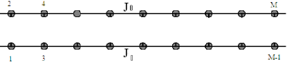
Figure 1: The non interacting system

At this stage the two legs are not interacting. Let us now close the chains imposing the following boundary conditions:

$$M+1\equiv 1\text{ \ , \ \ }M+2\equiv 2.$$ (5)

Depending on $M$, we get two topologically inequivalent boundary conditions: 1) for $M$ even, we get two independent $XXZ$ spin-1/2 chains, each one closed by gluing opposite ends: periodic boundary conditions (PBC); 2) for $M$ odd the two legs are not independent, indeed they appear to be connected at a point upon gluing the opposite ends and the system can be viewed as a single eight shaped chain. This local coupling is a source of local incommensuration, even in the absence of further interactions between up and down legs. Indeed, around the gluing point, an angle deviation is induced between the spins on the two chains from the decoupled value $\theta=\frac{\pi}{2}$ [18]. That defines a characteristic wavelength which is expected to be proportional to a finite correlation length $\xi_{spiral}$, $\theta-\frac{\pi}{2}\propto 1/\xi_{spiral}$, so it could give rise locally to a finite range spiral order. That is, for $M$ odd the system presents some kind of local topological defect in the gluing point, described by:

$$H_{0}^{MBC}=H_{0}+H_{MBC}$$

where the localized crossed interaction $H_{MBC}$ around the gluing point is explicitly given by:

$$H_{MBC}=J_{0}\sum_{i=M,M+1}(S_{i}^{x}S_{i+1}^{x}+S_{i}^{y}S_{i+1}^{y}+\Delta S_{i}^{z}S_{i+1}^{z})-J_{0}(S_{M}^{x}S_{M+2}^{x}+S_{M}^{y}S_{M+2}^{y}+\Delta S_{M}^{z}S_{M+2}^{z}).$$ (6)

This local deformation realizes the so called Mobius boundary conditions (MBC) in the system by physically introducing a topological defect at the gluing point. The system now exactly coincides with two closed $XXZ$ spin-1/2 chains, each one with $(M+1)/2$ sites, which intersect each other in the topological defect at site $M+1\equiv 1$. The existence of two topologically inequivalent configurations, which in the continuum are described by the two topological sectors, untwisted and twisted one, of our TM theory with central charge $c=2$ (see Section 5), is crucial in order to recognize an underlying topological order [34].

Now we are ready to introduce interactions between the two spin-1/2 $XXZ$ chains. Let us start from those which involve two spins, the railroad interaction:

$$H_{\text{Railroad}}=J_{\perp}^{R}\sum_{i=1}^{[(M+1)/2]}(S_{2i-1}^{x}S_{2i}^{x}+S_{2i-1}^{y}S_{2i}^{y}+\Delta S_{2i-1}^{z}S_{2i}^{z}),$$ (7)

and the zigzag one:

$$H_{\text{ZigZag}}=J_{\perp}^{Z}\sum_{i=1}^{M}(S_{i}^{x}S_{i+1}^{x}+S_{i}^{y}S_{i+1}^{y}+\Delta S_{i}^{z}S_{i+1}^{z}).$$ (8)

In order to briefly recall the relevant phenomenology due to such interactions, let us start with $H_{0}+H_{\text{Railroad}}$ [7] and discuss the isotropic $\Delta=1$ case (the system under study is depicted in Fig. 2).

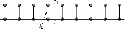
Figure 2: The railroad ladder

The weak coupling limit $J_{0}\gg\left|J_{\perp}^{R}\right|$ is interesting because it allows to study the crossover regime between the gapless spinon excitations on the two decoupled spin-1/2 chains and the strong coupling limit, which takes place when the energy scale is lowered [9]. The main universal features of the spectrum appear to be its symmetry and the persistence of a gap. Such a regime gives the opportunity to investigate the formation of massive spin $S=1$ and $S=0$ particles, which appear as bound states of the spin-1/2 excitations of the individual chains. Indeed, at small interchain coupling $\left|J_{\perp}^{R}\right|\ll J_{0}$ the masses of such particles are of the order of $\left|J_{\perp}^{R}\right|$, the $S=1$ branch being always lower. In the limit $\frac{J_{\perp}^{R}}{J_{0}}\rightarrow 0$ the singlet spectral gap results three times as large as the triplet one. Conversely, in the opposite limit $J_{\perp}^{R}\gg J_{0}$ the ground state is a product of rung singlets with a gap to the excited states which can be viewed as the energy needed in order to break a singlet bond. For $J_{\perp}^{R}\simeq J_{0}$ the energy gap still exists and the ground state is described by a short range valence-bond state [9][35]. In the strongly anisotropic case $\Delta=0$, for $J_{\perp}^{R}\gg J_{0}$ we get a rung singlet massive phase with a non degenerate ground state which is the direct product of singlets in the rung direction. Such a phase extends in the whole range of $J_{\perp}^{R}$, from very large values to very small ones, $J_{\perp}^{R}\simeq 0$ [35].

The zigzag ladder with Hamiltonian $H_{0}+H_{\text{ZigZag}}$ [18] [36][16] [37] (the system is shown in Fig. 3) is equivalent to the spin-1/2 frustrated Heisenberg chain with nearest neighbor coupling $J_{\perp}^{Z}$ and next to nearest neighbor coupling $J_{0}$.

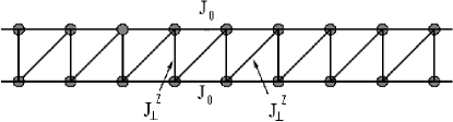
Figure 3: The zigzag ladder

In the isotropic case $\Delta=1$, such a model is shown to be critical for $J_{\perp}^{Z}>J_{\perp c}^{Z}$ ($J_{\perp c}^{Z}=J_{0}/0.241$) [38], being in the same universality class as the antiferromagnetic spin-1/2 Heisenberg chain. For $J_{\perp}^{Z}<J_{\perp c}^{Z}$ the spinons acquire a gap but remain still deconfined and the ground state becomes doubly degenerate [11]. Finally, at the Majumdar-Ghosh (MG) point [39] $J_{\perp}^{Z}=2J_{0}$, that is the exact dimerization point, the two degenerate ground states assume a simple form in the thermodynamic limit, being a collection of decoupled singlets as sketched in Fig. 4.

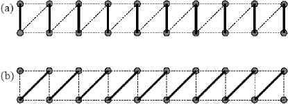
Figure 4: The two degenerate ground states of the zigzag ladder at the MG point

Such ground states can be continuously related to the rung singlet and Haldane phases [40]. For weaker interchain couplings $J_{\perp}^{Z}<2J_{0}$ incommensurate spiral correlations appear in the short range correlations [18][41]. In the regime $J_{0}\gg J_{\perp}^{Z}$ we may view the system as two spin chains with a weak zigzag interchain coupling [18][36]: an exponentially small gap develops and the weak interchain correlations break translational symmetry. So this phase shows a spontaneous dimerization along with a finite range incommensurate magnetic order. Exact diagonalizations as well as density matrix renormalization group (DMRG) calculations [42] have evidenced the difference between a zigzag ladder with an even and an odd number $M$ of sites respectively in the regime $J_{0}\gg J_{\perp}^{Z}$. In particular, for $M$ odd the $S=\frac{1}{2}$ ground state has a dispersion relation with a well defined single particle mode around $k=\frac{\pi}{2}$: such a particle can be viewed as a soliton whose gap increases exponentially when $J_{0}>$ $0.241$. Furthermore no soliton-antisoliton bound states form in this model and solitons are repelled by non magnetic impurities, that is by the ends of the open chains. Conversely, for $M$ even at the MG point there are exact singlet and triplet bound states in a small range of momenta close to $q=\frac{\pi}{2}$, which are degenerate.

In the strongly anisotropic case $\Delta=0$, two coupled $XX$ chains [16], the phase diagram is quite rich. Indeed for a small value of $J_{0}$ a spin fluid phase develops, characterized by gapless excitations with central charge $c=1$, while for $\frac{J_{0}}{J_{\perp}^{Z}}\simeq 0.32$ a phase transition of Kosterlitz-Thouless (KT) kind takes place and the system enters a massive dimerized phase with a twofold degenerate ground state. Conversely, in the large $J_{0}$ limit a critical spin nematic phase with chiral long range order develops. Such a non trivial phase with unbroken time-reversal symmetry is characterized by nonzero local spin currents polarized along the anisotropy $z$ axis. It preserves the spin $U\left(1\right)$ symmetry but spontaneously breaks the $Z_{2}$ symmetry. The transverse spin-spin correlation functions are incommensurate and fall off with the distance as a power law with exponent $\frac{1}{4}$. The ground state is characterized by longitudinal and transverse spin currents which are equal in magnitude but propagate in opposite directions. As a result local currents circulating around the triangular plaquettes of the ladder in an alternating way develop, the total spin current of the system being zero. That gives rise to two degenerate ground states characterized by an antiferromagnetic pattern of chiralities in adjacent plaquettes of the ladder, as shown in Fig. 5.

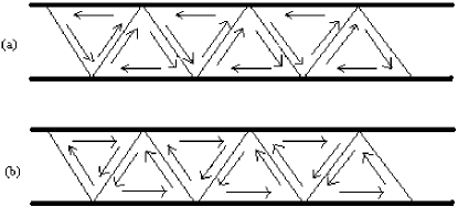
Figure 5: The two degenerate ground states of the zigzag $XX$ ladder in the spin nematic phase

Let us now introduce the closed geometry and point out the peculiarities which emerge in the interacting system for the two inequivalent configurations, $M$ even and odd. For $M$ even (PBC), the up and down legs of the ladder are still well distinguished even if coupled by the two interactions $H_{\text{Railroad}}$ and $H_{\text{ZigZag}}$; in this way the ground state structure and the nature of the excitations is preserved. Conversely, very different and more interesting features take place for $M$ odd (MBC). Indeed the zigzag interaction $H_{\text{ZigZag}}$ couples the $M$ site on the down leg with the $M+1\equiv 1$ site which still belongs to the down leg.

In the $\Delta=1$ case, that breaks the ground states structure and creates a domain-wall type defect in the system without loosing the translational invariance; such a topological defect can be viewed as a $S=\frac{1}{2}$ particle which is able to move with finite momentum. It has been shown [20] by Lanczos and Householder diagonalization methods that the defect particle gives rise to a single-spinon excitation in the spectrum. The presence of an isolated soliton in odd-length frustrated chains with a $S_{tot}=\frac{1}{2}$ ground state has been evidenced by DMRG methods as well [42]; in such a case the soliton excitation behaves as a massive free particle which is repelled by the ends of the chain, so it appears much more similar to a massive particle in a box. In the $\Delta=0$ case, we have that the alternating chiralities structure of the two ground states gets lost. Such a feature can be viewed as the localization of a topological defect which carries an elementary quantum of current, in full analogy with the half flux quantum associated with the topological defect in the closed Josephson junction ladder with MBC investigated in Refs. [27, 28, 29]: in this way the condition of zero total spin current in the ladder would be recovered. In presence of the railroad interaction we obtain more drastic effects, indeed the MBC turn locally on the $M+1\equiv 1$ site the interaction into a zigzag one. More precisely, the $1$ site interacts both with the $M$ site and the $2$ site and also with the $M-1$ site and the $3$ site via the Hamiltonian $H_{0}$.

The two spin interactions just introduced, $H_{\text{Railroad}}$ and $H_{\text{Zig-Zag}}$, can be described by means of a suitable unbalance of the zigzag interaction term. That is interesting in the continuum limit, because it is always possible to put together $H_{\text{Railroad}}$ and $H_{\text{Zig-Zag}}$ in a way to drop the marginal term which appears in $H_{\text{Railroad}}$ and obtain a pure relevant perturbation with conformal dimensions $(\frac{1}{2},\frac{1}{2})$ [9].

Let us now introduce the 4-spin interaction [10]:

$$H_{\text{4-Spin}}=J_{\epsilon}\sum_{i=1}^{[(M+1)/2]}\epsilon_{i}^{Dw}\epsilon_{i}^{Up},$$ (9)

which represents an interchain coupling of the spin-dimerization fields defined on the two legs of the ladder by:

$$\begin{array}[]{c}\epsilon_{i}^{Dw}=(-1)^{i}(S_{2i-1}^{x}S_{2i+1}^{x}+S_{2i-1}^{y}S_{2i+1}^{y}+\Delta S_{2i-1}^{z}S_{2i+1}^{z})\\ \epsilon_{i}^{Up}=(-1)^{i}(S_{2i}^{x}S_{2i+2}^{x}+S_{2i}^{y}S_{2i+2}^{y}+\Delta S_{2i}^{z}S_{2i+2}^{z})\end{array}.$$ (10)

That can be generated either by phonons or (in the doped state) by the conventional Coulomb repulsion between the holes.

Finally, let us introduce the following 8-spin interaction, termed 4-dimer:

$$H_{\text{4-Dimer}}=J_{\varkappa}\sum_{i=1}^{[(M+1)/2]}\varkappa_{i}\varkappa_{i+1},\text{ \ \ \ where: }\varkappa_{i}=\epsilon_{i}^{Dw}\epsilon_{i}^{Up}\text{.}$$ (11)

It plays a crucial role in the presence of the marginal interaction $H_{\text{Zig-Zag}}$ only, in that it gives rise to the dynamical generation of the triplet or singlet mass respectively along two different RG flows, in full analogy with the previous case of the relevant perturbations $H_{\text{Railroad}}$ and $H_{\text{4-Spin}}$.

The continuum limit of all interaction terms just introduced together with the different RG flows which originate by perturbing the two chain Hamiltonian $H_{0}$ (or $H_{0}^{MBC}$) is discussed in detail in Section 6, the continuum limit of $H_{0}$ (or $H_{0}^{MBC}$) being the subject of Section 5.

3 The XXZ spin-1/2 chain in the continuum limit

In this Section we briefly recall the Abelian bosonization technique for the description of the $XXZ$ spin-1/2 chain in the continuum limit. This quantum field theory is the starting point (mother theory, see next Section) in our TM description in the continuum of the 2-leg $XXZ$ spin-1/2 ladders arranged in a closed geometry. Of particular interest for us is the exact relation [32] between the compactification radius $R$ of the boson theory and the anisotropy parameter $\Delta$ of the chain; indeed the symmetry properties of TM crucially depend on this compactification radius. There is a wide literature on the subject of bosonization and on its applications, a review can be found in Ref. [31]; here, we summarize for clarity sake the main steps in the derivation [43].

Let us consider the single $XXZ$ spin-1/2 chain without magnetic field:

$$H_{XXZ}=J\sum_{j=1}^{N}(S_{j}^{x}S_{j+1}^{x}+S_{j}^{y}S_{j+1}^{y}+\Delta S_{j}^{z}S_{j+1}^{z}),$$ (12)

where $j$ is the site index, $N$ is the number of sites, $J>0$ is the exchange coupling and $\Delta$ is the anisotropy parameter. We can convert the above Hamiltonian to one of spinless interacting fermions on a lattice via the Jordan-Wigner transformation. Then, we linearize the energy spectrum around the Fermi surface and switch to the continuum limit by introducing right and left-moving bosons $\phi_{R}\left(x\right)$ and $\phi_{L}\left(x\right)$ (where $x=aj$, for lattice spacing equal to $a$). In this way the continuum limit of the Hamiltonian (12) reads:

$$H_{LL}=\frac{v_{F}}{8\pi}\int dx\left\{\left(1+g\right)\left[\left(\partial_{x}\phi_{R}\right)^{2}+\left(\partial_{x}\phi_{L}\right)^{2}\right]-2g\partial_{x}\phi_{L}\partial_{x}\phi_{R}\right\},$$ (13)

where only the marginal operators have been kept (see Section 3 of Ref. [44] for more details) and $g=\left(2J\Delta\sin^{2}k_{F}\right)/\pi v_{F}$, $v_{F}$ being the Fermi velocity. This is the exactly solvable Luttinger Hamiltonian:

$$H_{LL}=\frac{v}{8\pi}\int dx\left[\left(\partial_{x}\theta\right)^{2}+\left(\partial_{x}\phi\right)^{2}\right],$$ (14)

having introduced the bosonic field $\phi$ and its dual $\theta$, defined as:

$$\phi=\frac{\phi_{L}+\phi_{R}}{\sqrt{K}},\text{ }\theta=\sqrt{K}(\phi_{L}-\phi_{R}).$$ (15)

Here, the renormalized velocity $v$ and the Luttinger parameter $K$ are simply related to the parameters $g$ and $v_{F}$ by:

$$v=\frac{v_{F}}{2}\sqrt{1+2g},\text{ }K=1/\sqrt{1+2g}.$$ (16)

Moreover, they can be expressed in terms of the microscopic parameters $J$ and $\Delta$ by comparison with exact Bethe Ansatz calculations [32]:

$$v\left(\Delta\right)=\frac{J\pi}{2}\frac{\sqrt{1-\Delta^{2}}}{\arccos\Delta},\text{ \ \ \ \ \ }K\left(\Delta\right)=\frac{\pi}{2\left(\pi-\arccos\Delta\right)}.$$ (17)

In the standard bosonization framework, the spin operators have the following bosonic counterpart:

$$S_{j}^{z}\sim\sqrt{K}\partial_{x}\phi+(-1)^{j}const\times\cos(\sqrt{K}\phi),\text{ \ \ }S_{j}^{-}\sim e^{-\frac{i}{2\sqrt{K}}\theta}\left[(-1)^{j}+\cos(\sqrt{K}\phi)\right],$$ (18)

which, under the assumption of periodic boundary conditions, imply the compactification of the boson fields:

$$\phi(x+L,t) = \phi(x,t)+2\pi m_{\phi}R_{\phi},\text{ \ for }m_{\phi}\in\mathbb{Z}\text{ and }R_{\phi}=1/\sqrt{K},$$ (19)

$$\theta(x+L,t) = \theta(x,t)+2\pi m_{\theta}R_{\theta},\text{ \ for }m_{\theta}\in\mathbb{Z}\text{ and }R_{\theta}=2\sqrt{K}.$$ (20)

The compactification radii are functions only of the anisotropy parameter $\Delta$ while the Luttinger velocity $v$ (and analogously the lattice coupling $J$) enters as an overall factor in the spectrum. Such a consideration plays a crucial role in Section 5, in the construction of our TM and its relation with the $XXZ$ 2-leg ladder system. It is worth pointing out that the same compactification conditions can be derived on the basis of pure symmetry considerations [45].

Let us complete this Section by giving the mode expansion of the compactified boson field:

$$\phi(z,\bar{z})=q-ia_{0}\ln z-i\bar{a}_{0}\ln\bar{z}+\sum_{n\neq 0}\frac{ia_{n}}{n}z^{-n}+\sum_{n\neq 0}\frac{i\bar{a}_{n}}{n}\bar{z}^{-n}$$ (21)

in terms of the complex coordinates:

$$z=e^{2\pi(\tau-ix)/L},\text{ \ \ \ \ \ }\bar{z}=e^{2\pi(\tau+ix)/L},$$ (22)

where $\tau=ivt$ (Euclidean space-time). Here, the zero modes are:

$$a_{0}=p+w\text{ and }\bar{a}_{0}=p-w$$ (23)

where $w$ is the winding operator with eigenvalues $m_{\phi}R_{\phi}/2$ for $m_{\phi}\in\mathbb{Z}$ ($m_{\phi}$ is the winding number), $p$ is the conjugate momentum of $q$, $\left[q,p\right]=i,$ and the $a$-modes satisfy two independent Heisenberg algebras:

$$\left[a_{n},a_{n^{\prime}}\right]=n\delta_{n,n^{\prime}},\text{ \ \ \ }\left[a_{n},\bar{a}_{n^{\prime}}\right]=0,\text{ \ \ }\left[\bar{a}_{n},\bar{a}_{n^{\prime}}\right]=n\delta_{n,n^{\prime}}.$$ (24)

The compactification condition implies that the spectrum of the momentum $p$ is no-longer continuous but discrete with eigenvalues $n_{\phi}/R_{\phi}$ for $n_{\phi}\in\mathbb{Z}$. Finally, the Hamiltonian has the following mode expansion:

$$E=\frac{2\pi v}{L}\left\{\frac{1}{2}(a_{0}+\bar{a}_{0})+\sum_{n>0}a_{-n}a_{n}+\sum_{n>0}\bar{a}_{-n}\bar{a}_{n}\right\}.$$ (25)

4 $m$-reduction procedure on the plane

The $m$-reduction technique [33] is at the basis of the derivation of our Twisted Model (TM). Here, the main observation is that for any (mother) CFT, defined by a given chiral algebra, there exists a class of sub-theories (daughter theories) parameterized by an integer $m$ with the same algebraic structure but different central charge $c_{m}=mc$. The general characteristics of the daughter theory is the presence of twisted boundary conditions (TBC) which are induced on the component fields and are the signature of an interaction with a localized topological defect.

In this Section, contrary to our previous publications, we apply the $m$-reduction construction to scalar boson fields and not only to their chiral components. That is done in order to consider carefully the action of the $m$-reduction on the zero modes which, as shown in the following Section, will be crucial for the description of the antiferromagnetic 2-leg spin-1/2 $XXZ$ ladder with Mobius boundary conditions. In particular, we explicitly describe the $m$-reduction only for the $m=2$ case when the mother theory is the compactified boson theory ($c=1$), describing a single $XXZ$ spin-1/2 chain with general anisotropy parameter $\Delta$.

Let $\phi(z,\bar{z})$ be the compactified boson field of the mother theory, we can define the following two scalar fields:

$$\widetilde{\mathcal{X}}(\text{w},\text{\={w}})=\frac{\phi(\text{w},\text{\={w}})+\phi(e^{i\pi}\text{w},e^{-i\pi}\text{\={w}})}{\sqrt{2}},\text{ \ \ \ }\widetilde{\Phi}(\text{w},\text{\={w}})=\frac{\phi(\text{w},\text{\={w}})-\phi(e^{i\pi}\text{w},e^{-i\pi}\text{\={w}})}{\sqrt{2}},$$ (26)

which are respectively symmetric and antisymmetric under the action of the generator $g_{2}$: $($w,w̄$)\rightarrow(e^{i\pi}$w$,e^{-i\pi}$w̄$)$ of the discrete group $Z_{2}$. The $m=2$-reduction is implemented by the map $z=$w² which leads to the definition of the following daughter scalar fields:

$$\mathcal{X}(z,\bar{z})=\widetilde{\mathcal{X}}(z^{1/2},\bar{z}^{1/2})\text{ \ \ and \ \ }\Phi(z,\bar{z})=\widetilde{\Phi}(z^{1/2},\bar{z}^{1/2})\text{.}$$ (27)

The mode expansions of these last two fields are derived in terms of that of $\phi$, Eq.(21), and read as:

$$\mathcal{X}(z,\bar{z})=q_{0}-i\alpha_{0}\ln z-i\bar{\alpha}_{0}\ln\bar{z}+\sum_{n\in\mathbb{Z}-\{0\}}\frac{i\alpha_{n}}{n}z^{-n}+\sum_{n\in\mathbb{Z}-\{0\}}\frac{i\bar{\alpha}_{n}}{n}\bar{z}^{-n},$$ (28)

$$\Phi(z,\bar{z})=-\sqrt{2}\pi w+\sum_{n\in\mathbb{Z}}\frac{i\alpha_{n+1/2}}{n+1/2}z^{-(n+1/2)}+\sum_{n\in\mathbb{Z}}\frac{i\bar{\alpha}_{n+1/2}}{n+1/2}\bar{z}^{-(n+1/2)},$$ (29)

where:

$$q_{0}=\sqrt{2}(q+\pi w),\text{ \ }\alpha_{n+l/2}=\frac{a_{2n+l}}{\sqrt{2}},\text{ \ }\bar{\alpha}_{n+l/2}=\frac{\bar{a}_{2n+l}}{\sqrt{2}}\text{ \ \ with }n\in N\text{\ and }l=0,1\text{,}$$ (30)

and $w$ is the winding operator. The commutation relations of the daughter modes $\left\{q_{0},\{\alpha_{n+l/2}\},\{\bar{\alpha}_{n+l/2}\}\right\}$ follow from those of the mother modes $\left\{q,\{a_{n}\},\{\bar{a}_{n}\}\right\}$ and read as:

$$\left[\alpha_{n+l/2},\alpha_{n^{\prime}+l^{\prime}/2}\right]=\left(n+\frac{l}{2}\right)\delta_{n,n^{\prime}}\delta_{l,l^{\prime}},\text{\ \ }\left[\bar{\alpha}_{n+l/2},\bar{\alpha}_{{}_{n^{\prime}+l^{\prime}/2}}\right]=\left(n+\frac{l}{2}\right)\delta_{n,n^{\prime}}\delta_{l,l^{\prime}},$$ (31)

and

$$\left[\alpha_{n+l/2},\bar{\alpha}_{{}_{n^{\prime}+l^{\prime}/2}}\right]=0,\text{\ \ }\left[q_{0},\alpha_{n+l/2}\right]=i\delta_{0,n}\delta_{0,l},\text{ \ \ \ \ \ }\left[q_{0},\bar{\alpha}_{n+l/2}\right]=i\delta_{0,n}\delta_{0,l}.$$ (32)

Let us point out that the modes $\{\alpha_{n}\}_{n\in\mathbb{Z}}$ and $\{\bar{\alpha}_{n}\}_{n\in\mathbb{Z}}$ of the field $\mathcal{X}(z,\bar{z})$ define two independent standard Heisenberg algebras while those of the field $\Phi(z,\bar{z})$ ($\{\alpha_{n+1/2}\}_{n\in\mathbb{Z}}$ and $\{\bar{\alpha}_{n+1/2}\}_{n\in\mathbb{Z}}$) define two independent $Z_{2}$-twisted Heisenberg algebras with half-integer indices. The zero mode analysis shows that the field $\mathcal{X}(z,\bar{z})$ is a compactified boson with compactification radius $R_{\mathcal{X}}=R_{\phi}/\sqrt{2}$.

The description of the daughter theory proceeds now in a standard way. In particular, for both the $Z_{2}$ untwisted $\mathcal{X}$ and twisted $\Phi$ bosons we can define left and right chiral currents and components of the stress-energy tensor. Let us consider explicitly only the case of left chirality; the currents are:

$$J_{\mathcal{X}}(z)=i\partial_{z}\mathcal{X}(z,\bar{z})\left(=\sum_{n\in\mathbb{Z}}\alpha_{n}z^{-n}\right)\text{, \ }J_{\Phi}(z)=i\partial_{z}\Phi(z,\bar{z})\left(=\sum_{r\in\mathbb{Z}+1/2}\alpha_{r}z^{-r}\right),$$ (33)

and the corresponding components of the stress-energy tensor are:

$$T_{\mathcal{X}}(z)=-\frac{1}{2}\text{:}(\partial_{z}\mathcal{X})^{2}\text{: , \ \ \ \ }T_{\Phi}(z)=-\frac{1}{2}\text{:}(\partial_{z}\Phi)^{2}\text{:}+\frac{1}{16z^{2}}.$$ (34)

Notice that the second term in $T_{\Phi}(z)$ indicates that the $\Phi$-sector is built on the twisted vacuum generated by the left chiral twist field $\sigma(z)$ with conformal dimension $1/16$. That is also manifest in the mode expansion of the corresponding Virasoro generators:

$$L_{n}^{\mathcal{X}}=\frac{1}{2}\sum_{s\in\mathbb{Z}}\text{:}\alpha_{n-s}\alpha_{s}\text{:},\text{ \ \ \ }L_{n}^{\Phi}=\frac{1}{2}\sum_{r\in\mathbb{Z}+1/2}\text{:}\alpha_{n-r}\alpha_{r}\text{:}+\frac{\delta_{0,n}}{16}\text{ \ with }n\in\mathbb{Z.}$$ (35)

Let us stress that $\{L_{n}^{\Phi}\}$ and $\{L_{n}^{\mathcal{X}}\}$ define two independent Virasoro algebras both with central charge $c=1$. Thus the daughter theory has the left component of the stress-energy tensor equal to $T(z)=T_{\mathcal{X}}(z)+T_{\Phi}(z)$, which defines a Virasoro algebra with central charge $c=2$ ($m=2$-reduction).

5 2-leg $XXZ$ spin-1/2 ladders with Mobius boundary conditions: the continuum limit

In this Section we show how the TM, generated by $m=2$-reduction, describes well the 2-leg $XXZ$ spin-1/2 ladder with general anisotropy parameter $\Delta$ arranged in a closed geometry for PBC and MBC boundary conditions. The TM is characterized by two topological sectors, the untwisted and the twisted ones, which describe the continuum limit of the 2-leg $XXZ$ spin-1/2 ladder with PBC and MBC respectively. In order to establish that it is enough to show that the spin-1/2 $XXZ$ ladder with MBC in the continuum is naturally mapped in the twisted sector of our TM, i.e. the sector of TM generated by the $m=2$-reduction. Indeed the untwisted sector of TM can be described in terms of two untwisted boson fields, with the appropriate compactification radius, which define the continuum limit of the 2-leg $XXZ$ spin-1/2 ladder with PBC. Finally, the special value of the anisotropy parameter $\Delta=1$ is considered and the symmetry properties of the corresponding physical system briefly underlined.

Let us recall that the 2-leg $XXZ$ spin-1/2 ladder with $M$ odd sites and MBC coincides with a system of two $XXZ$ spin-1/2 chains, each one with $(M+1)/2$ sites, which are closed with periodicity condition in one gluing site which is common to the two chains. This induces a local deformation of the interaction which has a purely topological nature (topological defect) due to the fact that the gluing site has four nearest neighboring sites (two for each chain) with which it interacts. The presence of the topological defect implies that the ground state of the system in the thermodynamical limit is not in the sector $S_{tot}^{z}=0$. Indeed, while the full system has even size $L_{2}=2L$ ($L=a(M+1)/2$ being the size of the single chain and $a$ the lattice spacing) the number of quantum sites is the odd integer $M$. We can perform now a bosonization analysis for each chain of the system, as shown in Section 3. In this way we obtain, for the up and down chain respectively, two boson fields $\phi_{Up}$ and $\phi_{Dw}$ compactified on the two circles (up and down) of the same length $L$ and with the same compactification radius $R_{\phi}=\sqrt{2\left(\pi-\arccos\Delta\right)/\pi}$. Here, the presence of the topological defect implies the following boundary condition for the fields in the gluing point ($x_{Up}=x_{Dw}=0$):

$$\phi_{Up}(0,t)=\phi_{Dw}(0,t),$$ (36)

which in turn allows us to define the following folding field $\phi$ on the full system:

$$\phi(x,t)=\left\{\begin{array}[]{l}\phi_{Dw}(x,t),\text{ \ \ for }0\leq x\leq L,\\ \\ \phi_{Up}(x-L,t),\text{ \ \ for }L\leq x\leq 2L.\end{array}\right.$$ (37)

The non-trivial topology of the whole system is reflected into the fact that the points $x=0$ and $x=L$ coincide; that is, the compactification space of the field $\phi$ is not a circle of length $L_{2}$ but an eight of same length. It is now simple to show that on this eight-shaped space the field $\phi$ has compactification radius $R_{\phi}$. To this aim it is enough to observe that, on the up/down circle, starting from a given point $x_{Up/Dw}$ we come back to it under a shift of $L$ while, on the eight, we need a shift of $L_{2}=2L$, so that, it results:

$$\phi(x+2L,t)=\left\{\begin{array}[]{l}\phi_{Dw}(x+L,t),\text{ \ \ for }0\leq x\leq L,\\ \\ \phi_{Up}(x,t),\text{ \ \ for }L\leq x\leq 2L,\end{array}\right.$$

$$\text{\ \ \ \ \ \ \ \ \ \ \ \ \ \ \ \ \ \ \ \ \ \ \ \ \ \ \ \ \ \ \ \ \ }=\left\{\begin{array}[]{l}\phi_{Dw}(x,t)+2\pi m_{\phi}R_{\phi},\text{ \ \ for }0\leq x\leq L,\\ \\ \phi_{Up}(x-L,t)+2\pi m_{\phi}R_{\phi},\text{ \ \ for }L\leq x\leq 2L,\end{array}\right.$$

that is:

$$\phi(x+2L,t)=\phi(x,t)+2\pi m_{\phi}R_{\phi}\text{.}$$ (38)

Now we can introduce the complex coordinates:

$$\text{w}=e^{2\pi(\tau-ix)/L_{2}},\text{ \ \ \ \ \ \={w}}=e^{2\pi(\tau+ix)/L_{2}}$$ (39)

where $\tau=ivt$ (Euclidean space-time) and define the fields $\widetilde{\mathcal{X}}($w,w̄$)$ and $\widetilde{\Phi}($w,w̄$)$ according to the formula (26). Let us observe that on the square covering plane:

$$z=\text{w}^{2}=e^{2\pi(\tau-ix)/L},\text{ \ \ \ \ \ }\bar{z}=\text{\={w}}^{2}=e^{2\pi(\tau+ix)/L}$$ (40)

the coincidence of the points $x=0$ and $x=L$, required by the eight shape of the space in the $x$-coordinate, now holds automatically. In fact, the space in the $x$-coordinate is now a circle of length $L$. The above covering is nothing else but the map defined in the previous Section, which implements the $m=2$-reduction on the field $\phi($w,w̄$)$ producing the two independent boson fields $\mathcal{X}(z,\bar{z})$ and $\Phi(z,\bar{z})$ of the daughter theory.

Summarizing, by using the $m=2$-reduction technique, we have transformed the boson field $\phi$ compactified on the eight-shape space of length $2L$ with compactification radius $R_{\phi}$ into the two independent boson fields $\mathcal{X}$ and $\Phi$ compactified on a circle of length $L$, where $R_{\mathcal{X}}=R_{\phi}/\sqrt{2}$ is the compactification radius of $\mathcal{X}$. Thus the 2-leg $XXZ$ spin-1/2 ladder with general anisotropy parameter $\Delta$ and Mobius boundary conditions results described by the twisted sector of our TM.

Let us focus on the isotropic case, that is a $XXX$ ladder, corresponding to the value $\Delta=1$ of the anisotropy parameter. The mother theory now is a theory of a free massless boson field $\phi$ with central charge $c=1$, compactified on a circle with compactification radius $R_{\phi}^{2}=\frac{1}{K}=2$. As a result of the $2$-reduction procedure we obtain a $c=2$ theory of two boson fields, Eqs. (28) and (29), which describe the spin chains of the two legs. Such a daughter theory is an orbifold one, which decomposes into a tensor product of two CFTs, a twisted invariant one with $c=3/2$, realized by the boson $\mathcal{X}(z,\bar{z})$ and a Ramond Majorana fermion, while the second one has $c=1/2$ and is realized in terms of a Neveu-Schwarz Majorana fermion. Such a factorization, $\widehat{su(2)}_{2}\otimes($Ising$)$, is evident in the modular invariant partition function within the torus topology (95) (see Appendix A).

Let us notice that the non abelian bosonization model for the weakly coupled frustrated $XXX$ ladder, introduced in Ref. [36], with symmetry $\left(\text{Ising}\right)^{4}$ corresponds to only one topological sector of our orbifold theory, the untwisted one, which describes PBC imposed at the ends of the two spin-1/2 chains. In closed geometries, nevertheless, the appropriate theory has to include all the relevant boundary conditions, as MBC ones, and this is done by our TM due to the presence of the extra twisted sector. The different boundary conditions correspond to boundary states at the end of the finite ladder, which are codified in terms of the different sectors in the modular invariant partition function. The decomposition into two topological sectors just outlined gives rise to an essential difference in the low energy spectrum for the system under study. Indeed, in the untwisted sector (PBC) only two-spinon excitations are possible (i.e. $SU(2)$ integer spin representations) while, in the twisted sector (MBC) the presence of a topological defect provides a clear evidence of single-spinon excitations (i.e. $SU(2)$ half-integer spin representations). All that takes place in close analogy with fully frustrated Josephson ladders in the extremely quantum limit which are expected to map to spin-1/2 zigzag ladders [46].

6 Renormalization group analysis

In this Section we deal with the weakly interacting 2 leg spin-1/2 ladder system in the continuum by turning on the four different perturbations (7)-(9) and (11). We restrict our analysis to the isotropic case $\Delta=1$, and study the different renormalization group (RG) trajectories flowing from the UV fixed point, described by our TM.

It is worth recalling that our TM is a $Z_{2}$-orbifold with central charge $c=2$ and that the model described by standard bosonization technique coincides just with the untwisted sector of TM. In the next two subsections, we extend to the twisted sector of TM the RG analysis done previously in [9],[10] and [36] for the perturbations (7), (8) and (9). Moreover, in subsection 6.2, we introduce the new interaction (11) within its fermionic representation and study the RG flow generated by the combined action of the perturbations (8) and (11). Depending on the perturbing term, we obtain different infrared (IR) fixed points corresponding to different physical behaviors.

The perturbing terms are scalar ones and get expressed in terms of our bosonic daughter fields $\mathcal{X}(z,\bar{z})$ and $\Phi(z,\bar{z})$ and the corresponding dual fields $\mathcal{Y}(z,\bar{z})$ and $\Theta(z,\bar{z})$, which admit the following representation by left and right chiral components:

$$\mathcal{X}(z,\bar{z})=-iw_{\mathcal{X}}\ln\frac{z}{\bar{z}}+X(z)+\bar{X}(\bar{z}),\text{ \ \ }\mathcal{Y}(z,\bar{z})=X(z)-\bar{X}(\bar{z}),$$ (41)

and

$$\Phi(z,\bar{z})=-2\pi w_{\mathcal{X}}+\varphi(z)+\bar{\varphi}(\bar{z}),\text{ \ \ }\Theta(z,\bar{z})=\varphi(z)-\bar{\varphi}(\bar{z}),$$ (42)

where $w_{\mathcal{X}}$ is the winding operator with eigenvalues $m_{\mathcal{X}}R_{\mathcal{X}}/2$ and $m_{\mathcal{X}}\in\mathbb{Z}$. In the following a representation in terms of four Majorana fermion fields turns out useful, whose holomorphic components ${(1/2,0)}$ are defined as:

$$\psi_{1}(z)=\text{sin}X\left(z\right),\text{ }\psi_{2}(z)=\text{cos}X\left(z\right),\text{ }\psi_{3}(z)=\frac{\text{sin}\varphi\left(z\right)}{\sqrt{z}},\text{ }\psi_{0}(z)=\frac{\text{cos}\varphi\left(z\right)}{\sqrt{z}},$$ (43)

while the anti-holomorphic ones ${(0,1/2)}$ are:

$$\bar{\psi}_{1}(\bar{z})=-\text{sin}\bar{X}\left(\bar{z}\right),\text{ }\bar{\psi}_{2}(\bar{z})=\text{cos}\bar{X}\left(\bar{z}\right),\text{ }\bar{\psi}_{3}(\bar{z})=-\frac{\text{sin}\bar{\varphi}\left(\bar{z}\right)}{\sqrt{\bar{z}}},\text{ }\bar{\psi}_{0}(\bar{z})=\frac{\text{cos}\bar{\varphi}\left(\bar{z}\right)}{\sqrt{\bar{z}}}.$$ (44)

In the present case ($\Delta=1$), the TM is a $Z_{2}$-orbifold with $\widehat{su(2)}_{2}\otimes\bar{I}$ symmetry, where the Ising factor $\bar{I}$ (which is $Z_{2}$-antisymmetric) is generated by $\psi_{0}(z)$ (and the corresponding anti-holomorphic component $\bar{\psi}_{0}(\bar{z})$), and the $\widehat{su(2)}_{2}$ factor is generated by the currents:

$$J^{\pm}(z)=\psi_{3}(z)e^{\pm iX(z)},\text{ }J^{3}(z)=i\partial X(z),$$ (45)

and analogous expressions hold for the anti-holomorphic components. The Lagrangian describing the UV fixed point for the $XXX$ ladder is:

$$\mathcal{L}_{0}=\frac{1}{8\pi}(\partial_{\mu}\mathcal{X}\partial^{\mu}\mathcal{X}+\partial_{\mu}\Phi\partial^{\mu}\Phi)$$ (46)

while the perturbing terms $V$ depend on the particular system under study:

$$\mathcal{L}=\mathcal{L}_{0}-V.$$ (47)

6.1 Ladder and 4-Spin perturbations: massive flow

In the following we deal with the interacting terms $H_{\text{Railroad}}$, $H_{\text{4-Spin}}$, Eqs. (7) and (9), which we write in the continuum limit for the twisted sector of TM, retaining only the relevant terms.

In the continuum the railroad interaction gives rise to relevant perturbations (with conformal dimensions $(1/2,1/2)$) to the UV fixed point, described by our TM theory with central charge $c=2$. Such massive terms are given in terms of the boson fields (41)-(42) by:

$$V_{\text{Railroad}}=-m_{\text{R}}(\text{cos}\mathcal{X}(z,\bar{z})-\text{cos}\Phi(z,\bar{z})+2\text{cos}\Theta(z,\bar{z})),$$ (48)

where $m_{\text{R}}\varpropto J_{\perp}^{R}$,  $J_{\perp}^{R}$ being the coupling constant of the railroad interaction (7). In the Majorana fermion representation we get:

$$V_{\text{Railroad}}=-im_{\text{R}}\sum\limits_{i=1}^{3}\psi_{i}(z)\bar{\psi}_{i}(\bar{z})+3im_{\text{R}}\psi_{0}(z)\bar{\psi}_{0}(\bar{z}),$$ (49)

where it appears clearly that the $\psi_{i}$ ($i=1,2,3$) fields form an Ising triplet with the same mass $m_{\text{R}}$ (the $\widehat{su(2)}_{2}$ sector) and the remaining field is an Ising singlet (the $\bar{I}$ sector) with a larger mass $-3m_{\text{R}}$ [9].

Let us now switch on the 4-spin interaction $H_{\text{4-Spin}}$, Eq. (9), first introduced in Ref. [10], whose expression in the continuum limit can be found starting from the continuum limit for the dimerization operators:

$$\epsilon_{+}\sim\mu_{1}\mu_{2}\mu_{3}\sigma_{0},\ \ \ \ \epsilon_{-}\sim\sigma_{1}\sigma_{2}\sigma_{3}\mu_{0},$$ (50)

where $\epsilon_{\pm}=\epsilon_{Up}\pm\epsilon_{Dw}$ and $\epsilon_{Up/Dw}$ are the continuum analogues in the fermionic representation of the spin-field dimerizations corresponding to the up and down leg respectively, quoted in Eq. (10). Now, by using the fusion rules of the Ising model and dropping the most singular term, we can regularize the OPE lim${}_{z\rightarrow w}:\left(\epsilon_{+}(w,\bar{w})\epsilon_{+}(z,\bar{z})-\epsilon_{-}(w,\bar{w})\epsilon_{-}(z,\bar{z})\right):$ and write the continuum limit of the interaction $H_{\text{4-Spin}}$ as:

$$V_{\text{4-Spin}}(z,\bar{z})=im_{\epsilon}\sum\limits_{i=0}^{3}\psi_{i}(z)\bar{\psi}_{i}(\bar{z}).$$ (51)

Such a relevant mass term (with conformal dimensions $(1/2,1/2)$) can be rephrased in boson language as:

$$V_{\text{4-Spin}}=m_{\epsilon}(\text{cos}\mathcal{X}(z,\bar{z})+\text{cos}\Phi(z,\bar{z})),$$ (52)

where $m_{\epsilon}\varpropto J_{\epsilon}$, $J_{\epsilon}$ being the coupling constant of the 4-spin interaction $H_{\text{4-Spin}}$. As we see from Eq. (51), such a case is different from the railroad interaction (49) in that it gives rise to the same mass contribution $m_{\epsilon}$ for all the Ising fields $\psi_{i}$ ($i=0,1,2,3$). That allows the triplet or singlet mass to vanish also for finite (different from zero) values of the coupling constants $J_{\bot}^{R},J_{\epsilon}$, i.e. far from the UV conformal fixed point $c=2$.  Then two possible trajectories in the RG flow arise, the first characterized by ($m_{t}=0,m_{s}\neq 0$) and the second by ($m_{t}\neq 0,m_{s}=0$), where the mass different form zero increases more and more along the flow, while the vanishing one remains unchanged. In such a case the low energy spectrum is well described by an effective conformal field theory which is obtained after the decoupling of the massive component. We get two possible RG flows: a flow to an IR fixed point with central charge $c=3/2$ as a result of the Ising $\bar{I}$ decoupling and a flow to a different IR fixed point with central charge $c=1/2$ as a result of the $\widehat{su(2)}_{2}$ decoupling.

Let us now analyze the behavior of the staggered magnetization operator $n^{\pm}$ as well as the dimerization one $\epsilon_{\pm}$ along the massive RG flow just discussed. Within the $c=2$ theory they can be expressed in terms of the boson fields (41)-(42) as:

$$n^{+} \sim (\text{cos}\frac{\mathcal{Y}(z,\bar{z})}{2}\text{cos}\frac{\Theta(z,\bar{z})}{2},\text{ sin}\frac{\mathcal{Y}(z,\bar{z})}{2}\text{cos}\frac{\Theta(z,\bar{z})}{2},\text{ sin}\frac{\mathcal{X}(z,\bar{z})}{2}\text{cos}\frac{\Phi(z,\bar{z})}{2}),$$ (53)

$$n^{-} \sim (\text{sin}\frac{\mathcal{Y}(z,\bar{z})}{2}\text{sin}\frac{\Theta(z,\bar{z})}{2},\text{ cos}\frac{\mathcal{Y}(z,\bar{z})}{2}\text{sin}\frac{\Theta(z,\bar{z})}{2},\text{ cos}\frac{\mathcal{X}(z,\bar{z})}{2}\text{sin}\frac{\Phi(z,\bar{z})}{2}),$$ (54)

$$\epsilon_{+} \sim \text{cos}\frac{\mathcal{X}(z,\bar{z})}{2}\text{cos}\frac{\Theta(z,\bar{z})}{2},\ \ \ \ \ \ \epsilon_{-}\sim\text{sin}\frac{\mathcal{X}(z,\bar{z})}{2}\text{sin}\frac{\Theta(z,\bar{z})}{2}.$$ (55)

Indeed in the fermionic representation they are written as:

$$n^{+} \sim (\sigma_{1}\mu_{2}\sigma_{3}\sigma_{0},\mu_{1}\sigma_{2}\sigma_{3}\sigma_{0},\sigma_{1}\sigma_{2}\mu_{3}\sigma_{0}),\text{ \ \ }\epsilon_{+}\sim\mu_{1}\mu_{2}\mu_{3}\sigma_{0},$$ (56)

$$n^{-} \sim (\mu_{1}\sigma_{2}\mu_{3}\mu_{0},\sigma_{1}\mu_{2}\mu_{3}\mu_{0},\mu_{1}\mu_{2}\sigma_{3}\mu_{0}),\text{ \ \ }\epsilon_{-}\sim\sigma_{1}\sigma_{2}\sigma_{3}\mu_{0}.$$ (57)

In the disordered $\bar{I}$ Ising singlet phase characterized by $m_{s}>0$ ($m_{t}=0$) we get:

$$\langle\sigma_{0}\rangle=0,\text{ \ \ \ }\langle\mu_{0}\rangle\neq 0.$$ (58)

As a consequence the fields $\epsilon_{-}$ and $n^{-}$ can be expressed in terms of the primary fields of the CFT with $\widehat{su(2)}_{2}$ symmetry as:

$$n^{-}\sim(\mu_{1}\sigma_{2}\mu_{3},\sigma_{1}\mu_{2}\mu_{3},\mu_{1}\mu_{2}\sigma_{3}),\ \ \ \ \epsilon_{-}\sim\sigma_{1}\sigma_{2}\sigma_{3},$$ (59)

and the corresponding correlation functions of the relative staggered magnetization and dimerization field behave as:

$$\langle n^{-}(z)n^{-}(0)\rangle\sim\langle\epsilon_{-}(z)\epsilon_{-}(0)\rangle\sim\left|z\right|^{-3/4}.$$ (60)

Thus, the critical point $m_{t}=0$ is an IR fixed point with central charge $c=\frac{3}{2}$.

Likewise in the disordered $\widehat{su(2)}_{2}$ Ising triplet phase characterized by $m_{t}>0$ ($m_{s}=0$) we get:

$$\langle\sigma_{i}\rangle=0,\text{ \ \ \ }\langle\mu_{i}\rangle\neq 0\text{ \ \ }\forall i\in\{1,2,3\}.$$ (61)

As a consequence the field $\epsilon_{+}$ can be expressed in terms of the following primary field within the $\bar{I}$ CFT:

$$\epsilon_{+}\sim\sigma_{0},$$ (62)

and the corresponding correlation function follows a power law:

$$\langle\epsilon_{+}(z)\epsilon_{+}(0)\rangle\sim\left|z\right|^{-1/4}.$$ (63)

Thus the critical point $m_{s}=0$ belongs to the Ising universality class with central charge $c=\frac{1}{2}$ and signals a transition to a spontaneously dimerized phase with $\langle\epsilon_{+}\rangle\neq 0$.

6.2 Zigzag and 4-Dimer perturbations: massive flow

In the following we switch off the perturbing terms $H_{\text{Ladder}}$, $H_{\text{4-Spin}}$ and deal with the interacting terms $H_{\text{ZigZag}}$, $H_{\text{4-Dimer}}$, Eqs. (8) and (11), which we write in the continuum limit for the twisted sector of TM. Let us recall that the system of two spin-1/2 chains coupled via a zigzag interaction, with Hamiltonian $H_{0}+$ $H_{\text{ZigZag}}$, has been widely investigated in the literature [18][36][16][37] in the weak-coupling regime $J_{0}\gg J_{\perp}^{Z}$ via a non abelian bosonization approach[47]. In this limit of two quasi-decoupled chains with periodic boundary conditions, the system in the continuum has been described in terms of two level-1 Wess-Zumino-Witten (WZW) field theories or equivalently in terms of four Majorana fermions coupled by some perturbations. As a first step toward the RG analysis of the system in the presence of both the interactions (8) and (11), let us start extending the RG analysis of the system with only the zigzag interaction in the twisted sector of our TM. In the present case, the implementation of the continuum limit has to be brought out carefully, being eventually the zigzag interaction described by a marginal operator. The continuum limit of the Hamiltonian $H_{0}$ of two non-interacting chains leads to the free-fermion Lagrangian:

$$\mathcal{L}_{0}=\frac{1}{2\pi}\sum_{i=0}^{3}v_{i}\left(\psi_{i}\overline{\partial}\psi_{i}+\overline{\psi}_{i}\partial\overline{\psi}_{i}\right)$$ (64)

where $v_{0}=...=v_{3}=v\sim J_{0}a$ is the velocity of spin excitation in isolated chains, $a$ being the lattice spacing, plus a marginal interaction [36]:

$$V_{U}=-\lambda_{U}(O_{1}+O_{2}),$$ (65)

where $\lambda_{U}\sim U/|t|\geq 0$ and:

$$O_{1} = \psi_{1}(z)\bar{\psi}_{1}(\bar{z})\psi_{2}(z)\bar{\psi}_{2}(\bar{z})+\psi_{1}(z)\bar{\psi}_{1}(\bar{z})\psi_{3}(z)\bar{\psi}_{3}(\bar{z})+\psi_{2}(z)\bar{\psi}_{2}(\bar{z})\psi_{3}(z)\bar{\psi}_{3}(\bar{z}),$$ (66)

$$O_{2} = \psi_{0}(z)\bar{\psi}_{0}(\bar{z})(\psi_{1}(z)\bar{\psi}_{1}(\bar{z})+\psi_{2}(z)\bar{\psi}_{2}(\bar{z})+\psi_{3}(z)\bar{\psi}_{3}(\bar{z})),$$ (67)

within the Majorana fermion representation. The zigzag interaction $H_{\text{ZigZag}}$ has instead the following form:

$$V_{\text{ZigZag}}=\lambda_{\text{Z}}[(O_{1}-O_{2})+\sum_{i=0}^{3}(T^{(i)}(z)+\bar{T}^{(i)}(\bar{z}))],$$ (68)

where $\lambda_{\text{Z}}\sim J_{\perp}^{Z}/|t|\geq 0$ and $J_{\perp}^{Z}\geq 0$. Such an marginal interaction contains a non scalar term given by the sum over the energy-momentum tensor of the fermionic fields, whose effect is simply that of renormalizing the fields and the velocities:

$$\begin{array}[]{cc}\left(\psi_{i},\overline{\psi}_{i}\right)\rightarrow\frac{1}{\sqrt{1+\pi\lambda_{\text{Z}}}}\left(\psi_{i},\overline{\psi}_{i}\right)\mathcal{,}&i=0,1,2,3\end{array}$$ (70)

$$\begin{array}[]{cc}v_{0}\rightarrow v_{0}\frac{1+3\pi\lambda_{\text{Z}}}{1-3\pi\lambda_{\text{Z}}},&v_{i}\rightarrow v_{i}\frac{1-\pi\lambda_{\text{Z}}}{1+\pi\lambda_{\text{Z}}},i=1,2,3\end{array}.$$ (72)

After renormalization the whole effect of the perturbing terms $V_{\text{ZigZag}}$ and $V_{U}$ can be expressed as a marginal interaction:

$$\mathcal{V}_{\text{ZigZag}}=\lambda_{+}^{0}(O_{1}+O_{2})+\lambda_{-}^{0}(O_{1}-O_{2}),$$ (73)

where $\lambda_{\pm}^{0}=\frac{1}{2\left(1+\pi\lambda_{\text{Z}}\right)}\left\{\mp\frac{\lambda_{\text{Z}}+\lambda_{U}}{1-3\pi\lambda_{\text{Z}}}+\frac{\lambda_{\text{Z}}-\lambda_{U}}{1+\pi\lambda_{\text{Z}}}\right\}$ and satisfy the following RG equations [36]:

$$\frac{d\lambda_{\pm}^{0}}{d\ln L}=8\pi\left(\lambda_{\pm}^{0}\right)^{2}.$$ (74)

The value of the parameters $\lambda_{U}\geq 0$ and $\lambda_{\text{Z}}\geq 0$ gives rise to $\lambda_{+}^{0}<0$ and $\lambda_{-}^{0}$ small and positive. Thus, under the flow (74) $\lambda_{+}^{0}$ renormalizes to zero ($\lambda_{+}^{0}\rightarrow 0^{-}$) while $\lambda_{-}^{0}$ increases being marginally relevant and that results in a dynamical length scale $\xi\sim e^{1/\lambda_{-}^{0}}$. A mass scale appears dynamically and provides a non vanishing mass for the four fermions: $m_{i}\sim v_{i}\xi^{-1}$, $i=1,2,3$, $m_{0}\sim v_{0}\xi^{-1}$, with $m_{1}=m_{2}=m_{3}=m>0$, $m_{0}<-m$.

In such a picture it is not possible to extract trajectories in the RG flow characterized by a vanishing mass in the $c=1/2$ or $c=3/2$ sector respectively. In order to obtain such trajectories we need to introduce a new perturbing term, the 4-dimer $H_{\text{4-Dimer}}$, defined in Eq. (11). In the continuum the double dimerization operator $\varkappa_{i}=\epsilon_{i}^{Dw}\epsilon_{i}^{Up}$ can be defined by regularizing the following expression:

$$\varkappa(z,\bar{z})=\frac{C_{\varkappa}}{4}\text{ lim}_{z\rightarrow w}:\left(\epsilon_{+}(w,\bar{w})\epsilon_{+}(z,\bar{z})-\epsilon_{-}(w,\bar{w})\epsilon_{-}(z,\bar{z})\right):,$$ (75)

as done in the previous Subsection, Eq. (51); the net result is:

$$\varkappa(z,\bar{z})=\sum\limits_{i=0}^{3}\psi_{i}(z)\bar{\psi}_{i}(\bar{z})$$ (76)

The continuum limit of the interaction $H_{\text{4-Dimer}}$:

$$V_{\text{4-Dimer}}=\lambda_{\varkappa}(O_{1}+O_{2})=\lambda_{\varkappa}\sum\limits_{i\neq j=0}^{3}\psi_{j}(z)\bar{\psi}_{j}(\bar{z})\psi_{i}(z)\bar{\psi}_{i}(\bar{z}),$$ (77)

where $\lambda_{\varkappa}\sim J_{\varkappa}$, is now obtained applying once again the regularization procedure to the OPE lim${}_{z\rightarrow w}:\left(\varkappa(w,\bar{w})\varkappa(z,\bar{z})\right):$; the whole perturbation turns out to be:

$$\mathcal{V}_{\text{Tot}}\equiv\mathcal{V}_{\text{ZigZag}}+V_{\text{4-Dimer}}=\lambda_{+}(O_{1}+O_{2})+\lambda_{-}(O_{1}-O_{2})$$ (78)

where $\lambda_{+}=\lambda_{+}^{0}+\lambda_{\varkappa}$ and $\lambda_{-}=\lambda_{-}^{0}$. Such a general interaction contains two parameters, $\lambda_{+}$ and $\lambda_{-}$, which can be changed independently by changing the coupling constants ($J_{\perp}^{Z}$,$J_{\varkappa}$). In particular, that allows us to define a path in the RG flow characterized by a vanishing singlet mass, i.e. ($m_{t}\neq 0,m_{s}=0$). In order to obtain such a path let us rewrite the general perturbation (78) as:

$$\mathcal{V}_{\text{Tot}}=\Lambda_{1}O_{1}+\Lambda_{2}O_{2}$$ (79)

where $\Lambda_{1}=\lambda_{+}+\lambda_{-}$ and $\Lambda_{2}=\lambda_{+}-\lambda_{-}$. Notice that a mass $m_{s}$ for the singlet could be provided dynamically only by means of the interaction $O_{2}$, because of the presence of the term $\psi_{0}(z)\bar{\psi}_{0}(\bar{z})$. The vanishing of the singlet mass $m_{s}$ can then be obtained only by requiring the marginality of the operator $O_{2}$ along the RG flow. This selects out the condition $\lambda_{+}=\lambda_{-}$ which makes $\Lambda_{2}$ to vanish and which is left invariant under the RG equations. Within a self-consistent mean field approximation (see Appendix B), it is possible to show that along this RG flow trajectory the singlet mass $m_{s}$ indeed vanishes while the triplet mass $m_{t}$ is dynamically generated and reads:

$$m_{t}\sim\pm v_{t}\digamma\exp(-1/8\pi\lambda_{+}),$$ (80)

where $\digamma$ is a momentum cutoff and $v_{t}$ is the spin triplet velocity. The above analysis shows that, under the introduction of the 4-Dimer interaction, we are able to describe an RG trajectory flowing from our TM, the $c=2$ UV  fixed point, toward the Ising $\bar{I}$, the $c=1/2$ IR fixed point, as a result of the dynamical generation only of the triplet mass $m_{t}$ and the consequent decoupling of $\widehat{su(2)}_{2}$.

It is worth noting that the four interactions above introduced could not produce a massless flow to a conformal IR fixed point starting from the UV one with $c=2$. To this aim further interactions which could compete with the mass generation are needed. Let us mention here that following the same analysis developed in [30] we have that in the continuum limit the perturbation:

$$V_{3/2}=\sigma_{0}\sigma_{3},$$ (81)

gives rise to a massless RG flow to the $c=3/2$ IR fixed point, $\widehat{su(2)}_{2}$. The perturbing terms which induce in the continuum limit massless flows to the $c=1$ and $c=1/2$ fixed points can be similarly found and their lattice realization is under analysis.

7 Conclusions and outlooks

In this paper a complete CFT for antiferromagnetic spin-1/2 2-leg $XXZ$ ladders with general anisotropy parameter $\Delta$ and arranged in a closed geometry has been developed. Two kinds of boundary conditions on gluing the ends of the two legs have been considered, that is PBC and MBC. The two topologically inequivalent configurations which arise for an even and an odd number of sites in the ladder system are deeply investigated and the implications of the presence of a topological defect on the spectrum and the low-energy excitations are exploited. The net result in the continuum limit is a $Z_{2}$-orbifold CFT with central charge $c=2$, obtained through $2$-reduction on the single $XXZ$ antiferromagnetic spin-1/2 chain, whose topological sectors account well for the boundary conditions considered. In particular, in the twisted sector a single-spinon excitation to the conformal ground state arises which describes in the continuum the topological defect occurring in a closed ladder with MBC.

The role in determining different massive RG flows of the relevant interactions  ($H_{\text{Railroad}}$, $H_{\text{4-Spin}}$) and of the marginal relevant interactions ($H_{\text{ZigZag}}$, $H_{\text{4-Dimer}}$) is investigated in the isotropic ladder case with $\Delta=1$. In the four fermion description of the system, for both couples of interactions, the result is the possibility to generate massive RG flows with at will unbalanced fermion triplet ($m_{t}$) and singlet ($m_{s}$) masses. The fact that, at the conformal point, our TM model is the exact tensor product of the degrees of freedom of the fermion triplet (i.e. the affine $\widehat{su(2)}_{2}$, $c=3/2$) and of the singlet (i.e. the $\bar{I}$ Ising model, $c=1/2$ ) implies that along these RG flows the topological structure of TM is preserved. In fact, the TM global symmetry $su(2)\otimes Z_{2}$ cannot be broken by different values of the triplet and singlet masses, while it can be enhanced to a partial conformal one $\widehat{su(2)}_{2}\otimes Z_{2}$ or $su(2)\otimes\bar{I}$ along the special RG flows with $m_{t}=0$ or $m_{s}=0$, respectively. This stability allows us to follow the evolution of the single-spinon excitation while it acquires mass along a given RG flow. Thus, we can claim that the existence of massive single-spinon excitations is a general feature of closed ladders with MBC in the presence of various types of interactions. In the strong massive limit then such a single-spinon excitation should coincide with the one described in Ref. [20] in the special case of the zigzag interaction.

Finally, the possibility of getting a whole massless flow starting from the UV fixed point with central charge $c=2$ is briefly discussed. Further analysis on such an issue as well as the complete RG analysis for the anisotropic ladder with $\Delta=0$ will be the subject of a forthcoming publication. Another issue which deserves deeper investigation is the occurrence of a topological order in such spin ladders of non trivial geometry. That could result from the presence of a topological defect, in close analogy with the Josephson junction ladders studied in Refs. [27, 28, 29].

Appendix A: TM on the torus

In this Appendix we summarize the primary field content of our TM model on the torus topology for the particular case $m=2$ and for the compactification radius $R_{\phi}^{2}=2$ of the mother theory, which describes the 2-leg $XXX$ ladder. The decomposition of TM in terms of the $Z_{2}$-invariant (the affine $\widehat{su(2)}_{2}$ with $c=\frac{3}{2}$) and $Z_{2}$-twisted (the Ising model with $c=\frac{1}{2}$ ) sub-theories is well evidenced on the torus [1]  by the corresponding decomposition of the characters. In order to make it explicit let us start introducing the characters of these two RCFT. We denote with $\bar{\chi}_{0}(\tau)$, $\bar{\chi}_{\frac{1}{2}}(\tau)$, $\bar{\chi}_{\frac{1}{16}}(\tau)$ the characters of the chiral primary fields $I$, $\psi$ and $\sigma$ in the Ising model [48] with Neveu-Schwartz ($Z_{2}$-twisted) boundary conditions [1], while

$$\chi_{0}^{\widehat{su(2)}_{2}}(w|\tau) = \chi_{0}(\tau)K_{0}(w|\tau)+\chi_{\frac{1}{2}}(\tau)K_{2}(w|\tau)\,,$$ (82)

$$\chi_{1}^{\widehat{su(2)}_{2}}(w|\tau) = \chi_{\frac{1}{16}}(\tau)\left(K_{1}(w|\tau)+K_{3}(w|\tau)\right),$$ (83)

$$\chi_{2}^{\widehat{su(2)}_{2}}(w|\tau) = \chi_{\frac{1}{2}}(\tau)K_{0}(w|\tau)+\chi_{0}(\tau)K_{2}(w|\tau)$$ (84)

represent the characters of the three extended chiral primary fields in the affine $Z_{2}$-invariant $\widehat{su(2)}_{2}$. The characters $\chi_{0,2}^{\widehat{su(2)}_{2}}$ contain only integer spin (i.e. two-spinon excitations) while $\chi_{1}^{\widehat{su(2)}_{2}}$ describes half-integer spin (i.e. single-spinon excitations). The above character formulae express the decomposition of $\widehat{su(2)}_{2}$ in terms of the $c=1$ RCFT $\widehat{u(1)}_{4}$ (generated by the compactified boson $\mathcal{X}$ with $R_{\mathcal{X}}^{2}=1$) and in terms of the Ising model with Ramond boundary conditions. In particular, the $K_{l}(w|\tau)$ defined by [1]:

$$K_{l}(w|\tau)=\frac{1}{\eta\left(\tau\right)}\;\Theta\left[\begin{array}[]{c}\frac{l}{4}\\[6.0pt] 0\end{array}\right](2w|4\tau)\,,\qquad\text{with }l=0,1,2,3,$$ (85)

are the characters corresponding to the four extended chiral primary fields of the RCFT $\widehat{u(1)}_{4}$ while we denote with $\chi_{i}(\tau)$ those of the Ising model with Ramond boundary conditions.

We can write now the characters of TM, splitting them in the four sectors of the $Z_{2}$-orbifold. We have two extended chiral primaries in the $A-P$ sector with characters given by:

$$\chi_{0}^{+}(w|\tau) = \bar{\chi}_{\frac{1}{16}}(\tau)\left(\chi_{0}^{\widehat{su(2)}_{2}}(w|\tau)+\chi_{2}^{\widehat{su(2)}_{2}}(w|\tau)\right),$$ (86)

$$\chi_{1}^{+}(w|\tau) = \left(\bar{\chi}_{0}(\tau)+\bar{\chi}_{\frac{1}{2}}(\tau)\right)\chi_{1}^{\widehat{su(2)}_{2}}(w|\tau),$$ (87)

and two extended chiral primaries in the $A-A$ sector whose characters read:

$$\chi_{0}^{-}(w|\tau) = \bar{\chi}_{\frac{1}{16}}(\tau)\left(\chi_{0}^{\widehat{su(2)}_{2}}(w|\tau)-\chi_{2}^{\widehat{su(2)}_{2}}(w|\tau)\right),$$ (88)

$$\chi_{1}^{-}(w|\tau) = \left(\bar{\chi}_{0}-\bar{\chi}_{\frac{1}{2}}\right)(\tau)\chi_{1}^{\widehat{su(2)}_{2}}(w|\tau).$$ (89)

In the $P-A$ sector there are two extended chiral primaries with the following characters:

$$\tilde{\chi}_{0}^{-}(w|\tau) =\bar{\chi}_{0}(\tau)\chi_{0}^{\widehat{su(2)}_{2}}(w|\tau)-\bar{\chi}_{\frac{1}{2}}(\tau)\chi_{2}^{\widehat{su(2)}_{2}}(w|\tau),$$ (90)

$$\tilde{\chi}_{1}^{-}(w|\tau) =\bar{\chi}_{0}(\tau)\chi_{2}^{\widehat{su(2)}_{2}}(w|\tau)-\bar{\chi}_{\frac{1}{2}}(\tau)\chi_{0}^{\widehat{su(2)}_{2}}(w|\tau),$$ (91)

while for the $P-P$ sector we have three extended chiral primaries with characters given by:

$$\tilde{\chi}_{\alpha}^{+}(w|\tau) =\bar{\chi}_{0}(\tau)\chi_{0}^{\widehat{su(2)}_{2}}(w|\tau)+\bar{\chi}_{\frac{1}{2}}(\tau)\chi_{2}^{\widehat{su(2)}_{2}}(w|\tau)\,,$$ (92)

$$\tilde{\chi}_{\beta}^{+}(w|\tau) =\bar{\chi}_{0}(\tau)\chi_{2}^{\widehat{su(2)}_{2}}(w|\tau)+\bar{\chi}_{\frac{1}{2}}(\tau)\chi_{0}^{\widehat{su(2)}_{2}}(w|\tau),$$ (93)

$$\tilde{\chi}_{\gamma}^{+}(w|\tau) =\bar{\chi}_{\frac{1}{16}}(\tau)\chi_{1}^{\widehat{su(2)}_{2}}(w|\tau);$$ (94)

note that the above factorization expresses the parity selection rule ($m$-ality). It is interesting to point out that in the $P-P$ sector, unlike for the other sectors, modular invariance constraint requires the presence of three different characters. The isospin operator content of the character $\tilde{\chi}_{\gamma}^{+}(w|\tau)$ clearly evidences its peculiarity with respect to the other states of the periodic case. Indeed it is characterized by two twist fields ($\Delta=1/16$) in the isospin components. The occurrence of the double twist in such a state is simply due to periodicity. Indeed, being an isospin twist field the representation in the continuum limit of a single-spinon excitation, the double twist corresponds to a two-spinon excitation, typical of the periodic configuration.

Finally, it is possible to show (see [1]) that the diagonal partition function of the TM on the torus has the following factorized form:

$$Z(w|\tau)=Z^{\widehat{su(2)}_{2}}(w|\tau)Z_{\overline{I}}(\tau)\text{,}$$ (95)

in terms of the $\widehat{su(2)}_{2}$ partition function $Z^{\widehat{su(2)}_{2}}$ ($c=3/2$) and of the Ising partition function $Z_{\overline{I}}$ ($c=1/2$). They have, in turn, the following expression:

$$Z^{\widehat{su(2)}_{2}}(w|\tau) = |\chi_{0}^{\widehat{su(2)}_{2}}(w|\tau)|^{2}+|\chi_{1}^{\widehat{su(2)}_{2}}(w|\tau)|^{2}+|\chi_{2}^{\widehat{su(2)}_{2}}(w|\tau)|^{2},$$ (96)

$$Z_{\overline{I}}(\tau) = |\bar{\chi}_{0}(\tau)|^{2}+|\bar{\chi}_{\frac{1}{2}}(\tau)|^{2}+|\bar{\chi}_{\frac{1}{16}}(\tau)|^{2}.$$ (97)

Appendix B: mass analysis within the self-consistent mean field approximation

In this Appendix we carry out an analysis in a self-consistent mean field approximation for the masses $m_{t}$ and $m_{s}$. Our situation is more complex than the one quoted in Ref. [36] because we deal with the case where either $\lambda_{+}$ or $\lambda_{-}$ could be marginally relevant and provide a dynamical contribution to the singlet and triplet masses. So we need to keep track of a new feature: the spin singlet and triplet are in the presence of different interactions. Then we may write:

$$\psi_{0}(z)\bar{\psi}_{0}(\bar{z})\rightarrow i\varepsilon_{s}+\psi_{0}(z)\bar{\psi}_{0}(\bar{z}),\text{ \ \ }\psi_{j}(z)\bar{\psi}_{j}(\bar{z})\rightarrow i\varepsilon_{t}+\psi_{j}(z)\bar{\psi}_{j}(\bar{z}),\text{ \ }j=1,2,3,$$ (98)

where $\varepsilon_{s}$ and $\varepsilon_{t}$ can be a priori different. By substituting the expressions (98) in the general perturbing term $\mathcal{V}_{\text{Tot}}$, Eq. (79), and neglecting terms quartic in the fields $\psi$, we get:

$$\mathcal{V}_{\text{Tot}}=i\sum\limits_{i=1}^{3}m_{t}\psi_{i}(z)\bar{\psi}_{i}(\bar{z})+im_{s}\psi_{0}(z)\bar{\psi}_{0}(\bar{z})$$ (99)

where:

$$m_{t}=2\pi(2\varepsilon_{t}\Lambda_{1}+\varepsilon_{s}\Lambda_{2}),\text{ \ \ }m_{s}=6\pi\varepsilon_{t}\Lambda_{2}.$$ (100)

$\varepsilon_{t}$ and $\varepsilon_{s}$ may be determined self-consistently by using the expressions for the correlation functions of massive fermion fields; we get:

$$\varepsilon_{s}=m_{s}\int\frac{d^{2}k}{\pi}\frac{e^{-i\text{k}\cdot\text{x}}}{\text{k}^{2}+m_{s}^{2}}\text{ \ \ , \ }\varepsilon_{t}=m_{t}\int\frac{d^{2}k}{\pi}\frac{e^{-i\text{k}\cdot\text{x}}}{\text{k}^{2}+m_{t}^{2}}$$ (101)

with $m_{t}$ and $m_{s}$ replaced by the expressions given in Eqs. (100).

Along the special RG trajectory characterized by the condition $\Lambda_{2}=0$, the mass $m_{s}$ vanishes and the above system of equations reduces to the single equation in the triplet mass $m_{t}$:

$$\frac{m_{t}}{4\pi\Lambda_{1}}=m_{t}\int\frac{d^{2}k}{\pi}\frac{e^{-i\text{k}\cdot\text{x}}}{\text{k}^{2}+m_{t}^{2}}\text{ }$$ (102)

whose non-zero solution is given by (80).

References

- [1] G. Cristofano, G. Maiella, V. Marotta, Mod. Phys. Lett. A 15 (2000) 547; G. Cristofano, G. Maiella, V. Marotta, Mod. Phys. Lett. A 15 (2000) 1679; G. Cristofano, G. Maiella, V. Marotta, G. Niccoli, Nucl. Phys. B 641 (2002) 547; G. Cristofano, V. Marotta, G. Niccoli, JHEP 06 (2004) 056.
- [2] F. D. M. Haldane, Phys. Rev. Lett. 50 (1983) 1153; F. D. M. Haldane, Phys. Lett. A 93 (1983) 464.
- [3] D. C. Johnston, J. W. Johnson, D. P. Goshorn, A. J. Jacobson, Phys. Rev. B 35 (1987) 219; Z. Hiroi, M. Azuma, M. Takano, Y. Bando, J. Solid State Chem. 95 (1991) 230; E. Dagotto, Rep. Prog. Phys. 62 (1999) 1525.
- [4] E. Dagotto, T. M. Rice, Science 271 (1996) 618; Y. Wang, Phys. Rev. B 60 (1999) 9236.
- [5] K. Hida, J. Phys. Soc. Jpn. 63 (1994) 2359; T. Tonegawa, T. Nakao, M. Kaburagi, J. Phys. Soc. Jpn. 65 (1996) 3317; M. Oshikawa, M. Yamanaka, I. Affleck, Phys. Rev. Lett. 78 (1997) 1984; D. C. Cabra, A. Honecker, P. Pujol, Eur. Phys. J. B 13 (2000) 55.
- [6] N. Andrei, M. R. Douglas, A. Jerez, Phys. Rev. B 58 (1998) 7619; P. Azaria, P. Lecheminant, Nucl. Phys. B 575 (2000) 439; P. Azaria, P. Lecheminant, A. A. Nersesyan, Phys. Rev. B 58 (1998) R8881.
- [7] S. P. Strong, A. J. Millis, Phys. Rev. Lett. 69 (1992) 2419; S. P. Strong, A. J. Millis, Phys. Rev. B 50 (1994) 9911; M. Sigrist, T. M. Rice, F. C. Zhang, Phys. Rev. B 49 (1994) 12058; S. R. White, R. M. Noack, D. J. Scalapino, Phys. Rev. Lett. 73 (1994) 886.
- [8] D. J. Scalapino, Nature 377 (1995) 12; E. Dagotto, J. Riera, D. J. Scalapino, Phys. Rev. B 45 (1992) 5744.
- [9] D. G. Shelton, A. A. Nersesyan, A. M. Tsvelik, Phys. Rev. B 53 (1996) 8521; D. C. Cabra, A. Dobry, G. L. Rossini, Phys. Rev. B 63 (2001) 144408.
- [10] A. A. Nersesyan, A. M. Tsvelik, Phys. Rev. Lett. 78 (1997) 3939; Y. J. Wang, Phys. Rev. B 68 (2003) 214428.
- [11] F. D. M. Haldane, Phys. Rev. B 25 (1982) R4925; F. D. M. Haldane, Phys. Rev. B 26 (1982) 5257.
- [12] B. S. Shastry, B. Sutherland, Phys. Rev. Lett. 47 (1981) 964.
- [13] M. Azuma, Z. Hiroi, M. Takano, K. Ishida, Y. Kitaoka, Phys. Rev. Lett. 73 (1994) 3463; G. Castilla, S. Chakravarty, V. J. Emery, Phys. Rev. Lett. 75 (1995) 1823.
- [14] W. Shiramura, K. Takatsu, H. Tanaka, K. Kamishima, M. Takahashi, H. Mitamura, T. Goto, J. Phys. Soc. Jpn. 66 (1997) 1900.
- [15] W. Shiramura, K. Takatsu, B. Kurniawan, H. Tanaka, H. Uekusa, Y. Ohashi, K. Takizawa, H. Mitamura, T. Goto, J. Phys. Soc. Jpn. 67 (1998) 1548.
- [16] A. A. Nersesyan, A. O. Gogolin, F. H. L. Essler, Phys. Rev. Lett. 81 (1998) 910; P. Lecheminant, T. Jolicoeur, P. Azaria, Phys. Rev. B 63 (2001) 174426; T. Hikihara, M. Kaburagi, H. Kawamura, Phys. Rev. B 63 (2001) 174430.
- [17] E. Altman, A. Auerbach, Phys. Rev. Lett. 81 (1998) 4484.
- [18] S. R. White, I. Affleck, Phys. Rev. B 54 (1996) 9862.
- [19] S. Yunoki, J. Hu, A. L. Malvezzi, A. Moreo, N. Furukawa, E. Dagotto, Phys. Rev. Lett. 80 (1998) 845.
- [20] K. Okunishi, N. Maeshima, Phys. Rev. B 64 (2001) 212406.
- [21] U. Grimm, J. Phys. A: Math. Gen. 35 (2002) L25.
- [22] X. G. Wen, F. Wilczek, A. Zee, Phys. Rev. B 39 (1989) 11413; X. G. Wen, Phys. Rev. B 44 (1991) 2664; T. Senthil, M. P. A. Fisher, Phys. Rev. B 61 (2000) 9690; E. H. Kim, O. Legeza, J. Solyom, Phys. Rev. B 77 (2008) 205121.
- [23] X. G. Wen, Int. J. Mod. Phys. B 6 (1992) 1711; X. G. Wen, Adv. in Phys. 44 (1995) 405.
- [24] G. Cristofano, V. Marotta, A. Naddeo, Phys. Lett. B 571 (2003) 250.
- [25] G. Cristofano, V. Marotta, A. Naddeo, Nucl. Phys. B 679 (2004) 621.
- [26] G. Cristofano, V. Marotta, A. Naddeo, G. Niccoli, J. Stat. Mech.: Theor. Exper. (2006) L05002.
- [27] G. Cristofano, V. Marotta, A. Naddeo, J. Stat. Mech.: Theor. Exper. (2005) P03006.
- [28] G. Cristofano, V. Marotta, A. Naddeo, G. Niccoli, Eur. Phys. J. B 49 (2006) 83.
- [29] G. Cristofano, V. Marotta, A. Naddeo, G. Niccoli, Phys. Lett. A 372 (2008) 2464.
- [30] G. Cristofano, V. Marotta, P. Minnhagen, A. Naddeo, G. Niccoli, J. Stat. Mech.: Theor. Exper. (2006) P11009.
- [31] I. Affleck, in Fields, Strings and Critical Phenomena (Les Houches, Session XLIX), E. Brézin and J. Zinn-Justin (Eds.), Amsterdam: North-Holland (1988); A. O. Gogolin, A. A. Nersesyan, A. M. Tsvelick, Bosonization and Strongly Correlated Systems (Cambridge University Press, Cambridge, 1998); H. J. Schulz, Phys. Rev. B 34 (1986) 6372.
- [32] J. D. Johnson, S. Krinsky, B. M. McCoy, Phys. Rev. A 8 (1973) 2526; A. Luther, I. Peschel, Phys. Rev. B 12 (1975) 3908.
- [33] V. Marotta, J. Phys. A 26 (1993) 3481; V. Marotta, Mod. Phys. Lett. A 13 (1998) 853; V. Marotta, Nucl. Phys. B 527 (1998) 717; V. Marotta, Mod. Phys. Lett. A13 (1998) 2863.
- [34] G. Cristofano et al., work in preparation.
- [35] K. Hijii, A. Kitazawa, K. Nomura, Phys. Rev. B 72 (2005) 014449.
- [36] D. Allen, D. Senechal, Phys. Rev. B 55 (1997) 299.
- [37] C. Itoi, S. Qin, Phys. Rev. B 63 (2001) 224423.
- [38] K. Okamoto, K. Nomura, Phys. Lett. A 169 (1993) 433; S. Eggert, Phys. Rev. B 54 (1996) R9612.
- [39] C. K. Majumdar, D. K. Ghosh, J. Math. Phys. 10 (1969) 1388; C. K. Majumdar, D. K. Ghosh, J. Math. Phys. 10 (1969) 1399.
- [40] A. K. Kolezhuk, H. J. Mikeska, Phys. Rev. B 56 (1997) R11380.
- [41] T. Tonegawa, I. Harada, M. Kaburagi, J. Phys. Soc. Jpn. 61 (1992) 4665; R. Bursill, G. A. Gehring, D. J. J. Farnell, J. B. Parkinson, Tao Xiang, Chen Zeng, J. Phys.: Condens. Matt. 7 (1995) 8605; A. A. Aligia, C. D. Batista, F. H. L. Essler, Phys. Rev. B 62 (2000) 3259; O. Legeza, J. Solyom, L. Tincani, R. M. Noack, Phys. Rev. Lett. 99 (2007) 087203.
- [42] E. Sorensen, I. Affleck, D. Augier, D. Poilblanc, Phys. Rev. B 58 (1998) R14701.
- [43] T. Giamarchi, Quantum Physics in One Dimension, Clarendon Press, Oxford (2004).
- [44] R. G. Pereira, J. Sirker, J. S. Caux, R. Hagemans, J. M. Maillet, S. R. White and I. Affleck, J. Stat. Mech.: Theor. Exper. (2007) P08022.
- [45] S. Lukyanov and V. Terras, Nucl. Phys. B 654 (2003) 323.
- [46] Y. Nishiyama, Eur. Phys. J. B 17 (2000) 295.
- [47] I. Affleck, Nucl. Phys. B 265 (1986) 409; E. Witten, Comm. Math. Phys. 92 (1984) 455; A. B. Zamolodchikov, V. A. Fateev, Sov. J. Nucl. Phys. 43 (1986) 657; V. G. Knizhnik, A. B. Zamolodchikov, Nucl. Phys. B 247 (1984) 83.
- [48] P. Di Francesco, P. Mathieu, D. Senechal, Conformal Field Theories, Springer-Verlag, (1996).