Nonlinear dynamics of soft fermion
excitations in hot QCD plasma III:
Soft-quark bremsstrahlung and energy losses

$${\bf Abstract}$$

In general line with our early works [Yu.A. Markov, M.A. Markova, Nucl. Phys. A770 (2006) 162; 784 (2007) 443] within the framework of a semiclassical approximation the general theory of calculation of effective currents and sources generating bremsstrahlung of an arbitrary number of soft quarks and soft gluons at collision of a high-energy color-charged particle with thermal partons in a hot quark-gluon plasma, is developed. For the case of one- and two-scattering thermal partons with radiation of one or two soft excitations, the effective currents and sources are calculated in an explicit form. In the model case of ‘frozen’ medium, approximate expressions for energy losses induced by the most simple processes of bremsstrahlung of soft quark and soft gluon, are derived. On the basis of a conception of the mutual cancellation of singularities in the sum of so-called ‘diagonal’ and ‘off-diagonal’ contributions to the energy losses, an effective method of determining color factors in scattering probabilities, containing the initial values of Grassmann color charges, is suggested. The dynamical equations for Grassmann color charges of hard particle used by us early are proved to be insufficient for investigation of the higher radiative processes. It is shown that for correct description of these processes the given equations should be supplemented successively with the higher-order terms in powers of the soft fermionic field.

1 Introduction

In the third part of our work, we complete the analysis of dynamics of soft fermionic excitations in a hot QCD medium at the soft momentum scale started in [1, 2] (to be referred to as “Paper I” and “Paper II” throughout this text). Here we focus our attention on the study of soft quark bremsstrahlung of an high-energy color particle induced by collisions with thermal partons in a quark-gluon plasma (QGP). This energetic particle can be external one with respect to the medium or thermal (test) one and will be denoted by 1 in the subsequent discussion. For the sake of simplification, we consider the QGP confined in unbounded volume and all hard quark excitations will be thought massless.

Along the whole length of the paper we use notion of bremsstrahlung of soft quarks on equal terms with the commonly accepted that: bremsstrahlung of soft gluons. This makes it possible to achieve unified terminological unification for the radiative processes in QGP with hard and soft excitations of different statistics. Note that notion of radiation (or absorbtion) of soft fermion excitations by itself is not new. Such a terminology have been already used by Vanderheyden and Ollitrault [3] in analysis of contributions of soft sector of medium excitations to the damping rate of one-particle excitations in cold ultrarelativistic plasmas with QED and QCD interactions.

Let us take a brief look at our approach. It is based on a system of nonlinear integral equations for the gauge potential $A_{\mu}^{a}$ and the quark wave function $\psi_{\alpha}^{i}$, first obtained by Blaizot and Iancu [4]. The equations completely describe the dynamics of soft bose- and fermi-excitations of the medium and contain in the right-hand sides either color currents or color Grassmann-valued sources induced by both the medium and hard test particles. We supplement the Blaizot-Iancu equations by the generalized Wong equation describing a change of the classical color charge $Q=(Q^{a}),\,a=1,\ldots,N_{c}^{2}-1$ of a hard particle and also by the generalized equations for the Grassmann color charges $\theta^{\dagger}=(\theta^{\dagger i})$ and $\theta=(\theta^{i}),\,i=1,\ldots,N_{c}$. The latter equations enable us within the semiclassical approximation completely describe the dynamics of spin-$1/2$ hard particles. The generalization of these color charge evolution equations is connected with necessity of accounting interaction of the half-spin particles not only with soft gluon fields but with soft quark fields. Such approach to the description of dynamics of soft and hard excitations in the hot non-Abelian plasma proved to be rather productive. It has allowed to consider uniformly a wide range of phenomena that have already been demonstrated in Paper II and will be shown also in the present work.

We would like to elucidate those directions of theoretical research, where there can be useful the use of the approach outlined just above. The first of them is related with application to an effective theory of small-$x$ partons described by the classical equations of motion [5]. The strong gluon fields in the theory created by the classical color charge density $\rho^{a}$ carried by valence quarks inside the target large nucleus. In a number of works [6, 7] an approach permitting to express the $\rho^{a}$ in terms of the density of the classical color-charged particles moving in a non-Abelian background field has been developed. The color charges $Q^{a}$ of these particles satisfy the Wong equations. Such approach is valid in the dense regime when $\rho^{a}$ is assumed to be large.

Further in the work of Fukushima [8] attempt to take account of noncommutativity of the color charge density on the operator level, was made. This enables to allow possible quantum corrections. They may be now essential in the dilute regime in which generally quantum effects are not small. However, the effects of ‘noncommutativity’ in principle can appear also on a classical level if one supposes that in the system under consideration along with the classical gluon fields $A_{\mu}^{a}(x)$, the classical (stochastic) quark fields $\psi_{\alpha}^{i}(x)$ also can be generated. For the description of these effects it is necessary to introduce in addition to the usual color charge $Q^{a}$ the anticommuting Grassmann color charges $\theta^{\dagger i}$ and $\theta^{i}$ of hard particles also. Besides, in this case the equation of motion for the gluon field should be supplemented by the equation of motion for the quark field, where in the right-hand side of the latter there will be a color Grassmann-valued current (or source, in our terminology) expressed trough the $\theta$ charges. All this can enable to investigate more subtle effects, for example spin those, in the small $x$ physics already on the classical level of the description.

Another quite interesting direction, where there can be useful our ideas, is associated with construction of the general theory of non-Abelian fluid dynamics. In the paper of Bistrovic, Jackiw et al. [9] the simplest model for a color-conducting fluid in the presence of a chromoelectromagnetic field was suggested, namely it was written out the Euler equation with non-Abelian Lorentz force $nu^{\mu}Q^{a}F^{a}_{\mu\nu}$ on the right-hand side, where $Q^{a}=Q^{a}(t,{\bf x})$ is a space-time local non-Abelian charge satisfying a fluid Wong equation

$$[(D_{t}+{\bf v}\cdot{\bf D})\,Q]^{a}=0$$

with gauge covariant derivatives. The last equation is distinctive feature of the theory in question, reflecting the non-Abelian parallel transport structure. It is interesting to note that in spite of the fact that this theory has been aimed first of all at applications to the quark-gluon plasma, it has found application in other field of physics in research of the various spin transport phenomena in condensed matter physics [10].

The non-Abelian fluid flow is much richer by its property than familiar hydrodynamics. However, the structure of the theory still becomes more richer and diverse if one assumes that in the medium along with non-Abelian gauge field, ‘non-Abelian’ spinor field can be also induced. In this case, for example, instead of the fluid Wong equation written out above, according to (II.5.11) we will have now the following equation:

$$[(D_{t}+{\bf v}\cdot{\bf D})\,Q]^{a}=-ig\,[\vartheta^{\dagger i}(t^{a})^{ij}(\bar{\chi}_{\alpha}\psi_{\alpha}^{j}(t,{\bf x}))-(\bar{\psi}_{\alpha}^{j}(t,{\bf x})\chi_{\alpha})(t^{a})^{ji}\vartheta^{i}],$$

where $\theta^{i}=\theta^{i}(t,{\bf x})$ is a space-time local Grassmann non-Abelian charge and $\chi_{\alpha}=\chi_{\alpha}(t,{\bf x})$ is a space-time local spinor density which can be associated with usual microscopic spin density $S^{\mu\nu\lambda}$ [11]. By this means inserting the Grassmann charge density into consideration inevitably entails inclusion of a spin degree of freedom in general dynamics of the system (and vice versa) that is the qualitative new point in this theory.

Finally, the last direction which we would like to mention is connected with a study of the interaction processes of a jet with the medium at which can change the flavor of the jet, i.e. the flavor of the leading parton. Thus in the papers [12] it was shown that taking into account the effects of conversions between quark and gluon jets in traversing through the quark-gluon plasma is important along with energy losses to explain some experimental observations. In our approach the processes of jet conversions in the QGP is already ‘built into’ the formalism in fact a priory and they are its fundamental part. In [12] the flavor charging processes were considered only via two-body scattering of the type $gq\rightarrow qg,\,q\bar{q}\rightarrow gg,\,\ldots$ and serve as addition to the processes of energy losses. Our formalism enables to consider more complicated processes, where conversions of the jets are indissolubly related to radiative energy losses which are induced by soft quark bremsstrahlung. It is possible that such type of interactions of a jet with the hot QCD medium can give appreciable contribution to the flavor dependent measurements of jet quenching observables and finally to the final jet hadron chemistry.

The structure of the paper is as follows. In Section 2, the basic nonlinear integral equations on the gauge potential $A_{\mu}^{a}$ and the quark wave function $\psi_{\alpha}^{i}$ taking into account presence in the system under investigation of the color currents and the color Grassmann sources of two hard test particles, are written out. Examples of calculation of the simplest effective current and source generating bremsstrahlung of a soft gluon and a soft quark, respectively, are given. Section 3 is concerned with deriving formulae for the radiation intensity induced by the lowest-order bremsstrahlung processes considered in the previous section. In Section 4 and 5, the expressions for radiation intensity is analyzed in the context of the potential model and under the condition when the HTL-correction to bare two-quark – gluon vertex can be neglected. A rough formulae for the energy losses of a high-energy parton induced by the soft gluon and soft quark bremsstrahlung in the high-frequency and small-angle approximations are obtained. Section 6 presents the calculation of effective currents and sources generating bremsstrahlung of a soft gluon and a soft quark in the case of interaction of three hard test color-charged partons. It is shown that here there exist two different type of effective currents and effective sources, each of which is determined by the number of Grassmann charges $\theta^{\dagger}$ and $\theta$. Sections 7, 8, 9 are devoted to discussion of the role of so-called ‘off-diagonal’ contributions to gluon and quark radiation energies and their connection with double Born scattering. The algebraic equations representing the conditions of cancellation of singularities in the sum of ‘diagonal’ and ‘off-diagonal’ contributions to the energy loss of an energetic parton, are found. In Sections 10 and 11, details of calculation and analysis of various symmetry properties of the effective currents and sources defining a further type of high-order radiation processes, namely bremsstrahlung of two soft plasma excitations at collision of two hard test particles, are given. Bremsstrahlung of two soft gluons and bremsstrahlung of soft gluon and soft quark are considered in the former section while bremsstrahlung of a soft quark-antiquark pair and two soft quark are in the latter one. In Conclusion we briefly discuss two fundamentally different approaches to rigorous proof of the evolution equations for the color charges in external bosonic and fermionic fields which have been introduced in Paper II by semiphenomenological way: the complex WKB-Maslov approach and the world-line path integral one.

Finally, in Appendix A, an explicit form of medium modified quark propagator and scalar vertex functions deeply used in section 4 and 5, is written out. In Appendix B, the details of calculations of the trace arising in analysis of probability of soft quark bremsstrahlung in section 5 in the framework of static color center model, are given. In Appendixes C and D, an explicit form of the coefficient functions entering into the effective sources generating bremsstrahlung simultaneously of a soft gluon and a soft quark, and a soft quark-antiquark pair, is presented.

2 Lower order effective current and source

In this section we consider two examples of calculation of effective current and source to lowest nontrivial order in the coupling constant $g$, which generate processes of bremsstrahlung of soft gluon and soft quark, accordingly. Within the framework of semiclassical approximation, these effective quantities take into complete account additional degrees of freedom: soft and hard fermi-excitations.

At first we consider calculation of the effective current. As initial equation for construction of this and higher order effective currents one takes the nonlinear integral equation for a gauge potential $A_{\mu}^{a}(k)$ (II.3.3). We add two additional currents, namely, $j_{\theta\mu}^{\,a}[A,\bar{\psi},\psi](x)$ (Eq. (II.5.1)) and $j_{\Xi\,\mu}^{\,a}[A,\bar{\psi},\psi,Q_{0}](x)$ (Eq. (II.5.21)) to the right-hand side of the above-mentioned equation. Besides, it is necessary to consider the following simple circumstance: for the process of bremsstrahlung to take place, one needs at least two hard color-charged partons interacting among themselves in a medium. From what has been said, it might be assumed that the basic equation (in the momentum representation) for further analysis has the following form:

$$\,{}^{\ast}{\cal D}^{-1}_{\mu\nu}(k)A^{a\nu}(k)=-j^{A(2)a}_{\mu}(A,A)(k)-j^{\Psi(0,2)a}_{\mu}(\bar{\psi},\psi)(k)-j^{\Psi(1,2)a}_{\mu}(A,\bar{\psi},\psi)(k)$$

$$-\,\Bigl{\{}j^{(0)a}_{Q_{1}\mu}(k)+j^{(1)a}_{Q_{1}\mu}(A)(k)+j^{(2)a}_{Q_{1}\mu}(A,A)(k)+j_{\theta_{1}\mu}^{(1)a}(\bar{\psi},\psi)(k)$$ (2.1)

$$+\,j_{\theta_{1}\mu}^{(2)a}(A,\bar{\psi},\psi)(k)+\,j_{\Xi\,\mu}^{(2)a}(Q_{01},\bar{\psi},\psi)(k)+(1\rightarrow 2)\Bigr{\}}.$$

In what follows a high-energy particle 1 will be consider as external one with respect to the medium. It either is injected into the medium or is produced inside of the latter, whereas particle 2 (and also $3,\,4,\,\ldots$) is a thermolized particle (particles) with the typical energy of order of the temperature $T$. On the right-hand side of Eq. (2.1) in the expansion of the medium-induced currents $j^{A},\,j^{\Psi}$ and the currents of hard partons we have kept terms up to the third order in interacting fields $A_{\mu},\,\psi_{\alpha},\,\bar{\psi}_{\alpha}$ and initial values of color charges $Q_{0s}^{a},\,\theta_{0s}^{i},\,\theta_{0s}^{\dagger i},\;s=1,2$. Equation (I.3.3) defines an explicit form of the medium-induced currents $j^{A(2)a}_{\mu},\,j^{\Psi(0,2)a}_{\mu}$ and $j^{\Psi(1,2)a}_{\mu}$, and equations (II.3.4), (II.5.3) and (II.5.22) do explicit form of the hard particle currents $j^{(0)a}_{Q_{1}\mu},\,j^{(1)a}_{Q_{1}\mu},\ldots,j_{\theta_{1}\mu}^{(2)a},j_{\Xi\,\mu}^{(2)a}$, accordingly.

According to our conception the required lower order effective current is defined by derivation of the right-hand side of (2.1) with respect to initial values of Grassmann color charges $\theta_{01}^{\dagger i}$ and $\theta_{02}^{i}$ (or $\theta_{02}^{\dagger i}$ and $\theta_{01}^{i}$) at the point $A^{(0)a}_{\mu}=\psi^{(0)i}_{\alpha}=\dots=Q_{01}^{a}=Q_{02}^{a}=\theta_{01}^{\dagger i}=\ldots=0$, namely

$$\left.\left(\,\frac{\delta^{2}\!j^{\Psi(0,2)a}_{\mu}(\bar{\psi},\psi)(k)}{\delta\theta_{01}^{\dagger\,i}\,\delta\theta_{02}^{j}}+\,\frac{\delta^{2}\!j^{(1)a}_{\theta_{1}\mu}(\bar{\psi},\psi)(k)}{\delta\theta_{01}^{\dagger\,i}\,\delta\theta_{02}^{j}}+\,\frac{\delta^{2}\!j^{(1)a}_{\theta_{2}\mu}(\bar{\psi},\psi)(k)}{\delta\theta_{01}^{\dagger\,i}\,\delta\theta_{02}^{j}}\right)\right|_{\,0}\,$$

$$\equiv K^{a,\,ij}_{\mu}({\bf v}_{1},{\bf v}_{2};\chi_{1},\chi_{2};{\bf x}_{01},{\bf x}_{02}|\,k).$$

Here on the left-hand side, we have kept terms different from zero only. Taking into account Eqs. (I.3.3) and (II.5.3), from the last expression we easily find the desired effective current (more exactly, its part, see below)

$$K^{a,\,ij}_{\mu}({\bf v}_{1},{\bf v}_{2};\ldots|\,k)=\frac{g^{3}}{(2\pi)^{6}}\,(t^{a})^{ij}K_{\mu}({\bf v}_{1},{\bf v}_{2};\ldots|\,k),$$ (2.2)

where

$$K_{\mu}({\bf v}_{1},{\bf v}_{2};\ldots|\,k)\equiv K_{\mu}({\bf v}_{1},{\bf v}_{2};\chi_{1},\chi_{2};{\bf x}_{01},{\bf x}_{02}|\,k)$$ (2.3)

$$=-\!\int\left[\,\bar{\chi}_{1}\,{\cal K}_{\mu}({\bf v}_{1},{\bf v}_{2}|\,k,-q)\chi_{2}\right]\,{\rm e}^{-i({\bf k}-{\bf q})\cdot{\bf x}_{01}}{\rm e}^{-i{\bf q}\cdot{\bf x}_{02}}\,\delta(v_{1}\cdot(k-q))\delta(v_{2}\cdot q)dq,$$

and in turn

$${\cal K}_{\mu}({\bf v}_{1},{\bf v}_{2}|\,k,-q)$$ (2.4)

$$=\frac{v_{1\mu}}{(v_{1}\cdot q)}\,^{\ast}S(q)+\frac{v_{2\mu}}{v_{2}\cdot(k-q)}\,^{\ast}S(k-q)+\!\,^{\ast}S(k-q)\!\,^{\ast}\Gamma_{\mu}^{(G)}(k,-k+q,-q)\,^{\ast}S(q).$$

By this means we can write out the new effective current generating the simplest process of soft-gluon bremsstrahlung at collision of two hard partons with different statistics

$$K^{a}_{\mu}({\bf v}_{1},{\bf v}_{2};\ldots;\theta_{01},\theta_{02};\theta_{01}^{\dagger},\theta_{02}^{\dagger},\ldots|\,k)$$ (2.5)

$$=K^{a,\,ij}_{\mu}({\bf v}_{1},{\bf v}_{2};\ldots|\,k)\,\theta_{01}^{\dagger i}\theta_{02}^{j}+K^{a,\,ij}_{\mu}({\bf v}_{2},{\bf v}_{1};\ldots|\,k)\,\theta_{02}^{\dagger i}\theta_{01}^{j}.$$

The second term here is derived from the first one by the simple replacement $1\rightleftharpoons 2$ and thus complete symmetry of the current with respect to permutation of two hard particles is achieved. At the same time the given term provides a fulfilment of the requirement of reality for the current: $(\tilde{j}^{a}_{\mu}(k))^{\ast}=\tilde{j}^{a}_{\mu}(-k)$. In our case it leads to the following condition:

$$(K^{a,\,ij}_{\mu}({\bf v}_{1},{\bf v}_{2};\ldots|\,k))^{\ast}=K^{a,\,ji}_{\mu}({\bf v}_{2},{\bf v}_{1};\ldots|-\!k).$$ (2.6)

Making use explicit form of coefficient function (2.2) – (2.4) it is not difficult to verify that this condition is hold. In Fig. 1 diagrammatic interpretation of three terms on the right-hand side of Eq. (2.4) is presented.

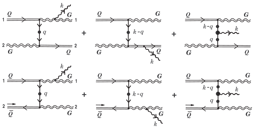
Figure 1: The simplest process of bremsstrahlung of soft gluon generated by color effective current (2.5). The blob stands for the HTL resummation, and the double lines denote hard particles. In the second line the annihilation channel of the process under consideration is given.

The current obtained (2.2) – (2.4) supplements similar one derived in our work [13] (Eqs. (2.11), (2.12)). The effective current in [13] defines the process of soft-gluon bremsstrahlung without a change of statistics of the colliding hard particles.

Proceed now to calculation of an effective source generating the simplest process of bremsstrahlung of soft quark. As the initial equations for construction of effective sources one takes the nonlinear integral equations for the soft-quark interacting fields $\psi_{\alpha}^{i}$ and $\bar{\psi}_{\alpha}^{i}$ (II.3.10). To the right-hand side of these equations we add all additional sources (II.5.14), (II.5.18) and (II.5.19) induced by hard partons 1 and 2. Also it is necessary to add another additional source which has not been taken into account in Paper II (see accepted there notations)

$$\hskip 56.9055pt\eta_{\tilde{\Omega}\,\alpha}^{i}(x)=\tilde{\beta}_{1}\,g\,\chi_{\alpha}(t^{a})^{ii_{1}}\,\Omega^{i_{1}}(t)\Bigl{[}\,\theta^{\dagger j}(t)(t^{a})^{jj_{1}}\,\Omega^{j_{1}}(t)\Bigr{]}\,{\delta}^{(3)}({\bf x}-{\bf v}t),$$

where $\tilde{\beta}_{1}$ is some new constant. As a result, we have in the momentum representation

$$\,{}^{\ast}\!S^{-1}_{\alpha\beta}(q)\psi^{i}_{\beta}(q)=-\,\eta^{(1,1)\,i}_{\alpha}(A,\psi)(q)-\eta^{(2,1)\,i}_{\alpha}(A,A,\psi)(q)$$ (2.7)

$$-\,\Big{\{}\eta^{(0)i}_{\theta_{1}\alpha}(q)+\,\eta^{(1)i}_{\theta_{1}\alpha}(A)(q)+\,\eta^{(2)i}_{\theta_{1}\alpha}(A,A)(q)+\,\eta^{(0,1)i}_{Q_{1}\alpha}(\psi)(q)+\,\eta^{(1,1)i}_{Q_{1}\alpha}(A,\psi)(q)$$

$$+\,\,\eta^{(2)i}_{\Xi\alpha}(\bar{\psi},\psi,\theta_{01})(q)+\,\eta^{(2)i}_{\Omega\alpha}(\bar{\psi},\psi,\theta_{01})(q)+\,\eta^{(2)i}_{\tilde{\Omega}\alpha}(\psi,\psi,\theta_{01}^{\dagger})(q)+\,(1\rightarrow 2)\Bigr{\}}.\hskip 8.5359pt$$

A similar equation is valid for $\bar{\psi}_{\alpha}^{i}(q)$. Here, on the right-hand side in the expansion of the medium induced sources $\eta,\,\bar{\eta}$, and sources $\eta_{\theta_{1,2}},\,\eta_{Q_{1,2}},\,\eta_{\Xi}$, $\eta_{\Omega}$ and $\eta_{\tilde{\Omega}}$ induced by hard particles 1 and 2, we have kept the terms up to the third order in interacting fields and initial values of Grassmann $\theta^{i}_{0\,1,2}$, $\theta^{\dagger i}_{0\,1,2}$ and usual $Q_{0\,1,2}^{a}$ color charges. Equation (I.3.4) defines an explicit form of the medium-induced sources $\eta^{(1,1)\,i}_{\alpha}(A,\psi)(q)$, $\eta^{(2,1)\,i}_{\alpha}(A,A,\psi)(q)$. Furthermore, eq. (II.3.11) defines an explicit form of the sources $\eta^{(0)i}_{\theta_{1,2}\,\alpha}(q)$, $\eta^{(1)i}_{\theta_{1,2}\,\alpha}(A)(q)$ and $\eta^{(2)i}_{\theta_{1,2}\,\alpha}(A,A)(q)$, and equations (II.4.3), (II.5.15), (II.5.20) do an explicit form of the sources $\eta^{(0,1)i}_{Q_{1}\alpha},\,\eta^{(2)i}_{\Xi\alpha},$ and $\eta^{(2)i}_{\Omega\alpha}$, respectively. Finally, an explicit form of the new source $\eta^{(2)i}_{\tilde{\Omega}\alpha}$ is defined as follows:

$$\eta^{(2)i}_{\tilde{\Omega}\alpha}(\psi,\psi,\theta_{1}^{\dagger})(q)=\frac{g^{3}}{2(2\pi)^{3}}\,\tilde{\beta}_{1}\,\theta_{01}^{\dagger j}\!\left[(t^{a})^{ii_{1}}(t^{a})^{ji_{2}}-(t^{a})^{ii_{2}}(t^{a})^{ji_{1}}\right]$$

$$\times\!\int\!\frac{\chi_{1\alpha}}{(v_{1}\cdot q_{1})(v_{1}\cdot q_{2})}\,(\bar{\chi}_{1}\psi^{i_{1}}(q_{1}))(\bar{\chi}_{1}\psi^{i_{2}}(q_{2}))\,\delta(v_{1}\cdot(q-q_{1}-q_{2}))dq_{1}dq_{2}.$$

The first nontrivial effective color source arises by differentiating the right-hand side of Eq. (2.7) with respect to usual color charge $Q_{01}^{a}$ and Grassmann color one $\theta_{02}^{j}$

$$\left.\left(\frac{\delta^{2}\eta^{(1,1)i}_{\alpha}(A,\psi)(q)}{\delta Q_{01}^{a}\,\delta\theta_{02}^{j}}\,+\,\frac{\delta^{2}\eta^{(1)i}_{\theta_{2}\alpha}(A)(q)}{\delta Q_{01}^{a}\,\delta\theta_{02}^{j}}\,+\,\frac{\delta^{2}\eta^{(1)i}_{Q_{1}\alpha}(\psi)(q)}{\delta Q_{01}^{a}\,\delta\theta_{02}^{j}}\right)\!\right|_{\,0}$$

$$\equiv K^{a,\,ij}_{\alpha}({\bf v}_{1},{\bf v}_{2};\chi_{1},\chi_{2};{\bf x}_{01},{\bf x}_{02}|\,q),$$

where on the left-hand side one again has kept the terms that give nonzero contributions. Taking into account Eqs. (I.3.4), (II.3.11) and (II.5.14), from the above expression we find the following effective source:

$$K^{a,\,ij}_{\alpha}({\bf v}_{1},{\bf v}_{2};\ldots|\,q)=\frac{g^{3}}{(2\pi)^{6}}\,(t^{a})^{ij}K_{\alpha}({\bf v}_{1},{\bf v}_{2};\ldots|\,q).$$ (2.8)

Here,

$$K_{\alpha}({\bf v}_{1},{\bf v}_{2};\ldots|\,q)\equiv K_{\alpha}({\bf v}_{1},{\bf v}_{2};\chi_{1},\chi_{2};{\bf x}_{01},{\bf x}_{02}|\,q)$$ (2.9)

$$=\int\!{\cal K}_{\alpha}({\bf v}_{1},{\bf v}_{2};\chi_{1},\chi_{2}|\,q,-q_{1})\,{\rm e}^{-i({\bf q}-{\bf q}_{1})\cdot{\bf x}_{01}}{\rm e}^{-i{\bf q}_{1}\cdot{\bf x}_{02}}\,\delta(v_{1}\cdot(q-q_{1}))\delta(v_{2}\cdot q_{1})dq_{1},$$

and

$${\cal K}_{\alpha}({\bf v}_{1},{\bf v}_{2};\chi_{1},\chi_{2}|\,q,-q_{1})=-\,\alpha\,\frac{\chi_{1\alpha}}{(v_{1}\cdot q_{1})}\;[\bar{\chi}_{1}\,^{\ast}S(q_{1})\chi_{2}]-\frac{\chi_{2\alpha}}{v_{2}\cdot(q-q_{1})}\,(v_{2\mu}\!\,^{\ast}{\cal D}_{C}^{\mu\nu}(q-q_{1})v_{1\nu})$$

$$+\,v_{1\mu}\!\,^{\ast}{\cal D}_{C}^{\mu\nu}(q-q_{1})\!\,^{\ast}\Gamma_{\nu,\;\alpha\beta}^{(Q)}(q-q_{1};q_{1},-q)\,^{\ast}S_{\beta\beta^{\prime}}(q_{1})\chi_{2\beta^{\prime}}.$$ (2.10)

Now we write out the most general form of the effective source generating the simplest process of soft quark bremsstrahlung at collision of two hard partons. This source is symmetric with respect to the permutation of hard particles $1\rightleftharpoons 2$

$$K^{i}_{\alpha}({\bf v}_{1},{\bf v}_{2};\ldots;\theta_{01},\theta_{02};Q_{01},Q_{02};\ldots|\,q)$$ (2.11)

$$=K^{a,\,ij}_{\mu}({\bf v}_{1},{\bf v}_{2};\ldots|\,q)\,Q_{01}^{a}\theta_{02}^{j}+K^{a,\,ij}_{\alpha}({\bf v}_{2},{\bf v}_{1};\ldots|\,q)\,Q_{02}^{a}\theta_{01}^{j}.$$

In Fig. 2 diagrammatic interpretation of the first term on the right-hand side of Eq. (2.11) is presented. The coefficient function here is defined by formulae (2.8) – (2.10). Because this contribution is proportional to usual color charge $Q_{01}^{a}$, the type of a hard parton 1 is the same as at the beginning of interaction so at the end (similar statement holds for contribution with charge $Q_{02}^{a}$). Let us specially note that this circumstance is the general rule. Every term of an expansion of effective current or source containing an usual color charge $Q_{0s}^{a},\,s=1,2,3,\ldots$ defines the scattering process in which statistics of hard parton $s$ does not change at the external legs. The same is true whenever in the expansion there is a combination Grassmann color charges of the type $\theta_{0s}^{\dagger i}\theta_{0s}^{j},(not\;summation!)\,s=1,2,3,\ldots\,.$ On the other hand, if in the expansion there exist ‘not compensated’ Grassmann charges: $\theta_{0s}^{i},\,\theta_{0s}^{\dagger i},\theta_{0s}^{i}Q_{0s}^{a},\theta_{0s}^{\dagger i}Q_{0s}^{a}$, and so on, then it suggests that the hard parton $s$ changes its own statistics during interaction.

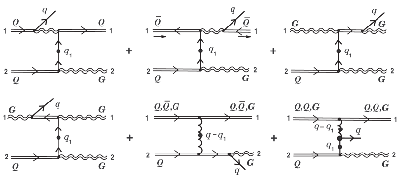
Figure 2: The simplest process of bremsstrahlung of soft quark generated by effective Grassmann source (2.8). Here the first four diagrams are associated with the first term on the right-hand side of Eq. (2.10).

3 Radiation intensity of soft gluon and soft quark bremsstrahlung

In the expression for lowest order effective current (2.5) without loss of generality one can set ${\bf x}_{01}=0$ and choose the vector ${\bf x}_{02}$ in the form ${\bf x}_{02}=({\bf b},z_{02})$, where two-dimensional vector ${\bf b}$ is orthogonal to the relative velocity ${\bf v}_{1}-{\bf v}_{2}$. Besides, in an subsequent discussion the longitudinal component $z_{02}$ also does not play any role and thus it can be set equal to zero. The energy of soft gluon radiation field generated by some effective current, is defined by the following general expression:

$$W({\bf b})=-(2\pi)^{4}\!\int\!d{\bf k}d\omega\!\int\!dQ_{01}dQ_{02}\,\omega\,{\rm Im}\,\left\langle\tilde{j}^{\ast a}_{\mu}(k;{\bf b})\!\,^{\ast}{\cal D}^{\mu\nu}_{C}(k)\tilde{j}^{a}_{\nu}(k;{\bf b})\right\rangle.$$ (3.1)

Here,

$$dQ_{01,\,2}=\delta(Q_{01,\,2}^{b}Q_{01,\,2}^{b}-C_{2}^{(1,\,2)})\prod_{a=1}^{d_{A}}\!dQ_{01,\,2}^{a},\quad d_{A}=N_{c}^{2}-1$$

with the second order Casimir $C_{2}^{(1,\,2)}$ for 1 or 2 hard color particles; $\langle\cdot\rangle$ is an expectation value over an equilibrium ensemble and $\!\,{}^{\ast}{\cal D}^{\mu\nu}_{C}(k)$ is medium modified gluon propagator in the Coulomb gauge. In the rest of frame of the medium the propagator has the following structure:

$$\,{}^{\ast}{\cal D}^{00}_{C}(k)=\biggl{(}\frac{k^{2}}{{\bf k}^{2}}\biggr{)}\,^{\ast}\!\Delta^{l}(k);\quad\,^{\ast}{\cal D}^{0i}(k)=0,$$ (3.2)

$$\,{}^{\ast}{\cal D}^{ij}_{C}(k)=(\delta^{ij}-k^{i}k^{j}/{\bf k}^{2})\,^{\ast}\!\Delta^{t}(k)\equiv\sum_{\zeta=1,2}{\rm e}^{\ast i}(\hat{\bf k},\zeta)\,{\rm e}^{j}(\hat{\bf k},\zeta),\quad\hat{k}^{i}\equiv k^{i}/|{\bf k}|$$

where $\,{}^{\ast}\!\Delta^{l,\,t}(k)=1/(k^{2}-\Pi^{l,\,t}(k))$ are scalar longitudinal and transverse propagators.

Let us substitute effective current (2.5) into the right-hand side of Eq. (3.1). Taking into account (3.2) and normalization

$$\int\!dQ_{01}=\int\!dQ_{02}=1,$$

from Eq. (3.1) we find

$$W({\bf b})=-\,\frac{1}{(2\pi)^{2}}\,\biggl{(}\frac{{\alpha}_{s}}{\pi}\biggr{)}^{\!3}C_{\theta\theta}^{(1;\,2)}\!\!\sum_{\xi=1,2\,}\!\int\!d{\bf k}d\omega\,\omega\,{\rm Im}(^{\ast}{\!\Delta}^{t}(k))$$ (3.3)

$$\times\left\{|\,{\rm e}^{i}(\hat{\bf k},\xi)K^{i}({\bf v}_{1},{\bf v}_{2};{\bf b}|-\!k)|^{\,2}+|\,{\rm e}^{i}(\hat{\bf k},\xi)K^{i}({\bf v}_{1},{\bf v}_{2};{\bf b}|\,k)|^{\,2}\right\}$$

$$\hskip 52.63777pt-\,\frac{1}{(2\pi)^{2}}\,\biggl{(}\frac{{\alpha}_{s}}{\pi}\biggr{)}^{\!3}C_{\theta\theta}^{(1;\,2)}\!\!\int\!d{\bf k}d\omega\,\omega\,\biggl{(}\frac{k^{2}}{{\bf k}^{2}}\biggr{)}{\rm Im}(^{\ast}{\!\Delta}^{l}(k))$$

$$\times\left\{|\,K^{0}({\bf v}_{1},{\bf v}_{2};{\bf b}|\,-\!k)|^{\,2}+|\,K^{0}({\bf v}_{1},{\bf v}_{2};{\bf b}|\,k)|^{\,2}\right\},$$

$\alpha_{s}\equiv g^{2}/4\pi.$ Here, for the sake of brevity we have introduced notation for the color factor

$$C_{\theta\theta}^{(1;2)}\equiv(\theta_{01}^{\dagger}t^{a}\theta_{02})(\theta_{02}^{\dagger}t^{a}\theta_{01}).$$

This color factor under conjugate turns into itself and therefore it can be consider as some real number (in particular, this enables us to take $C_{\theta\theta}^{(1;2)}$ outside the imaginary part sign in (3.1)). Its explicit value will be defined in section 7. Note that in deriving (3.3) we have used the condition of reality (2.6) for the effective current under investigation. This provides us a possibility of resulting initial expression for the energy of radiation field in form more convenient for analysis of the model case of ‘frozen’ thermal partons.

Let us now turn to formula for radiation intensity of bremsstrahlung of soft gluon. In our paper [13] we have used the following expression for the radiation intensity:

$${\cal I}=\!\!\sum\limits_{\zeta=Q,\,\bar{Q},\,G}\int\!\frac{d{\bf p}_{2}}{(2\pi)^{3}}\,f_{{\bf p}_{2}}^{(\zeta)}\Biggl{(}\int\!d{\bf b}\,W({\bf b};\zeta)|\,{\bf v}_{1}-{\bf v}_{2}|\Biggr{)}\equiv\left\langle\frac{dW({\bf b})}{dt}\right\rangle_{\!{\bf b}},$$ (3.4)

where $f_{{\bf p}_{2}}^{(\zeta)}$ are the distribution functions of thermal particles. We emphasize that here summation is taken over all types of hard partons: massless quark, antiquark and gluon. We also have taken into consideration that the energy of radiation field $W({\bf b})$ depends on $\zeta$ itself through color factors. Therefore here, one has used the notation $W({\bf b};\zeta)$ instead of $W({\bf b})$.

However, the case when we consider explicitly the fermion degree of freedom of the system is somewhat more complicated. Formula (3.4) just holds in case of condition when an effective current (by means of which the radiation energy $W({\bf b};\zeta)$ is defined) contains the usual color charge $Q^{a}_{02}$ (or the product $Q^{a}_{02}Q^{a_{1}}_{02}\ldots Q^{a_{n}}_{02}$) of a thermal parton 2. It is precisely this simplest case has been studied in detail in our early work [13]. On the other hand if an effective current contains Grassmann charges $\theta_{02}^{i},\,\theta_{02}^{\dagger i}$ or their combinations $\theta_{02}^{\dagger i}\theta_{02}^{j}$, $Q_{02}^{a}\theta_{02}^{i}$, $Q_{02}^{a}\theta_{02}^{\dagger i}$ and so on, then it is necessary to use the following expression for the radiation intensity (Paper II):

$${\cal I}=\!\!\sum\limits_{\zeta=Q,\,\bar{Q}}\int\!\frac{d{\bf p}_{2}}{(2\pi)^{3}}\,\left[f_{{\bf p}_{2}}^{(\zeta)}+f_{{\bf p}_{2}}^{(G)}\right]\Biggl{(}\int\!d{\bf b}\,W({\bf b};\zeta)|\,{\bf v}_{1}-{\bf v}_{2}|\Biggr{)}\equiv\left\langle\frac{dW({\bf b})}{dt}\right\rangle_{\!{\bf b}}.$$ (3.5)

Here the summation is taken over thermal quarks and antiquarks only. By virtue of the above-mentioned, to provide correct radiation intensity induced by effective current (2.5), it is necessary to make use the second expression (3.5). Let us substitute (3.3) into (3.5). The modules squared in the integrand in (3.3) are analyzed using explicit structure (2.3) in full analogy with similar expressions in [13]. As the final result we obtain the following expression for soft gluon radiation intensity

$$\left\langle\frac{dW({\bf b})}{dt}\right\rangle_{{\!{\bf b}}}^{\!{\cal F}}=-\biggl{(}\frac{{\alpha}_{s}}{\pi}\biggr{)}^{\!3}\Biggl{(}\sum\limits_{\;\zeta=Q,\,\bar{Q}}\!\!C_{\theta\theta}^{(1;\zeta)}\!\!\int\!{\bf p}_{2}^{2}\left[f_{|{\bf p}_{2}|}^{(\zeta)}+f_{|{\bf p}_{2}|}^{(G)}\right]\frac{d|{\bf p}_{2}|}{2\pi^{2}}\,\Biggr{)}$$ (3.6)

$$\times\,\Biggl{[}\int\!\frac{d\Omega_{{\bf v}_{2}}}{4\pi}\!\sum_{\xi=1,\,2\,}\int\!d{\bf k}d\omega\,\omega\,{\rm Im}(^{\ast}{\!\Delta}^{t}(k))$$

$$\times\!\int\!d{\bf q}\,\Bigl{\{}|\,\bar{\chi}_{1}({\rm e}^{i}(\hat{\bf k},\xi){\cal K}^{i}({\bf v}_{1},{\bf v}_{2}|\,k,-q))\chi_{2}|^{\,2}\,\delta(\omega-{\bf v}_{2}\cdot{\bf q}-{\bf v}_{1}\cdot({\bf k}-{\bf q}))$$

$$\hskip 48.36958pt+\,|\,\bar{\chi}_{1}({\rm e}^{i}(\hat{\bf k},\xi){\cal K}^{i}({\bf v}_{1},{\bf v}_{2}|\,-\!k,-q))\chi_{2}|^{\,2}\,\delta(\omega+{\bf v}_{2}\cdot{\bf q}-{\bf v}_{1}\cdot({\bf k}+{\bf q}))\Bigr{\}}$$

$$+\,\Bigl{(}\,^{\ast}{\!\Delta}^{t}(k)\rightarrow\,^{\ast}{\!\Delta}^{l}(k),\;{\rm e}^{i}{\cal K}^{i}\rightarrow\sqrt{\frac{k^{2}}{{\bf k}^{2}}}\,{\cal K}^{0}\Bigr{)}\Biggr{]}_{q^{0}=({\bf v}_{2}\cdot\,{\bf q})}.$$

It is necessary to stress that whereas the ${\cal K}^{i}$ amplitude depends only on velocity ${\bf v}_{2}\,\,({\bf v}_{2}^{2}=1)$ of thermal partons, the $|\,{\bf p}_{2}|$ - dependence of the integrand in (2.6) implicitly enters through spinor $\chi_{2}$ (see Appendix C in Paper II and footnote in the next section). For this reason it is impossible to fulfill the integration over $d|{\bf p}_{2}|$ in the first line of Eq. (3.6). The symbol ${\cal F}$ on the left-hand side of the above equation denotes ‘fermionic’ contribution to the soft-gluon radiation intensity, which should be added to similar ‘bosonic’ contribution (Eq. (3.9) in work [13]).

To determine the radiation intensity caused by bremsstrahlung of real quantum of oscillations it is sufficient in the case of a weak-absorption medium to approximate an imaginary part of scalar propagators in (3.6) in the following way

$${\rm Im}(^{\ast}{\!\Delta}^{t,\,l}(k))\simeq-\pi\,{\rm sign}(\omega)\,\frac{{\rm Z}_{t,\,l}({\bf k})}{2\omega_{\bf k}^{t,\,l}}\,[\,\delta(\omega-\omega_{\bf k}^{t,\,l})+\delta(\omega+\omega_{\bf k}^{t,\,l})],$$ (3.7)

where ${\rm Z}_{t,\,l}({\bf k})$ are the residues of appropriate scalar propagators ${}^{\ast}{\!\Delta}^{t,\,l}(k)$ at the relevant poles and $\omega_{\bf k}^{t,\,l}\equiv{\omega}^{t,\,l}({\bf k})$ are the dispersion relations for transverse and longitudinal modes. In substituting the last expression into (3.6) it is necessary to drop the term containing $\delta(\omega+\omega_{\bf k}^{t,\,l})$ since it corresponds to absorption process rather then to radiation one.

Now we turn to determine of an expression for intensity radiation of soft quark bremsstrahlung generated by effective source (2.11). The energy of soft quark radiation field $\psi_{\alpha}^{i}(q)=-\,^{\ast}\!S_{\alpha\beta}(q)\,\tilde{\eta}_{\beta}^{i}[A^{(0)},\psi^{(0)}](q;\,{\bf b})$ is defined as follows:

$$W({\bf b})=-\,\frac{i}{2}\,\,(2\pi)^{4}\!\!\int\!d{\bf q}dq^{0}\,q^{0}\!\int\!\!dQ_{01}dQ_{02}\,\left\langle\bar{\tilde{\eta}}^{i}(-q;{\bf b})\bigr{\{}\,^{\ast}\!S(-q)+\!\,^{\ast}\!S(q)\bigl{\}}\,\tilde{\eta}^{i}(q;{\bf b})\right\rangle$$ (3.8)

$$=(2\pi)^{4}\!\!\int\!d{\bf q}dq^{0}\,q^{0}\!\int\!\!dQ_{01}dQ_{02}\,\Bigl{\{}\,{\rm Im}\,(\!\,^{\ast}\!\Delta_{+}(q))\left\langle\bar{\tilde{\eta}}^{i}(-q;{\bf b})\,h_{+}(\hat{\bf q})\,\tilde{\eta}^{i}(q;{\bf b})\right\rangle$$

$$\hskip 150.79968pt+\,\,{\rm Im}\,(\!\,^{\ast}\!\Delta_{-}(q))\left\langle\bar{\tilde{\eta}}^{i}(-q;{\bf b})\,h_{-}(\hat{\bf q})\,\tilde{\eta}^{i}(q;{\bf b})\right\rangle\Bigr{\}}.$$

On the most-right hand side we have used an representation of the quark propagator $\,{}^{\ast}\!S(q)$ through the scalar propagators $\Delta_{\pm}(q)$, Eq. (A.1).

Let us substitute effective source (2.11) into the right-hand side of the preceding equation. Taking into account averaging rules over initial values of usual color charges

$$\int\!dQ_{01}\,Q_{01}^{a}Q_{01}^{b}=\frac{C_{2}^{(1)}}{d_{A}}\,\delta^{ab},\quad\int\!dQ_{02}\,Q_{02}^{a}Q_{02}^{b}=\frac{C_{2}^{(2)}}{d_{A}}\,\delta^{ab}$$

and also representation of the $h_{\pm}(\hat{\bf q})$ ‘projectors’ in terms of eigenspinors of chirality and helicity

$$(h_{+}({\hat{\bf q}}))_{\alpha\beta}=\sum\limits_{\lambda=\pm}u_{\alpha}(\hat{\bf q},\lambda)\bar{u}_{\beta}(\hat{\bf q},\lambda),\quad(h_{-}({\hat{\bf q}}))_{\alpha\beta}=\sum\limits_{\lambda=\pm}v_{\alpha}(\hat{\bf q},\lambda)\bar{v}_{\beta}(\hat{\bf q},\lambda),$$

from (3.8) we find

$$W({\bf b})=$$ (3.9)

$$=\frac{1}{(2\pi)^{2}}\,\biggl{(}\frac{{\alpha}_{s}}{\pi}\biggr{)}^{\!3}\Biggl{\{}C^{(2)}_{\theta}\Biggl{(}\frac{C_{F}\,C_{2}^{(1)}}{d_{A}}\Biggr{)}\!\sum\limits_{\lambda=\pm}\int\!d{\bf q}dq^{0}\,q^{0}\,{\rm Im}\,(\!\,^{\ast}\!\Delta_{+}(q))|\,\bar{u}(\hat{\bf q},\lambda)K({\bf v}_{1},{\bf v}_{2};\ldots;{\bf b}|\,q)|^{\,2}$$

$$\hskip 79.6678pt+\,C^{(1)}_{\theta}\Biggl{(}\frac{C_{F}\,C_{2}^{(2)}}{d_{A}}\Biggr{)}\!\sum\limits_{\lambda=\pm}\int\!d{\bf q}dq^{0}\,q^{0}\,{\rm Im}\,(\!\,^{\ast}\!\Delta_{+}(q))|\,\bar{u}(\hat{\bf q},\lambda)K({\bf v}_{2},{\bf v}_{1};\ldots;{\bf b}|\,q)|^{\,2}\Biggr{\}}$$

$$\hskip 42.67912pt+\,\Bigr{(}\,^{\ast}{\!\Delta}_{+}(q)\rightarrow\,^{\ast}{\!\Delta}_{-}(q),\;\bar{u}(\hat{\bf q},\lambda)\rightarrow\bar{v}(\hat{\bf q},\lambda)\Bigr{)}\biggl{\}}.$$

Here, $C^{(1)}_{\theta}\equiv\theta_{01}^{\dagger i}\theta_{01}^{i},\,C^{(2)}_{\theta}\equiv\theta_{02}^{\dagger i}\theta_{02}^{i}$ are constants. Their explicit form have been defined in Paper II; $C_{F}=(N_{c}^{2}-1)/2N_{c}$. Making use (3.9) we will determine just below the soft quark radiation intensity. All the above-mentioned reasoning concerning a correct choice of formula for the radiation intensity of soft gluon bremsstrahlung holds for soft quark bremsstrahlung also. In this particular case of effective source (2.11) the situation is somewhat more complicated in comparison with effective current (2.5). In the latter case both terms in the right-hand side of (2.5) contain Grassmann charges of a hard thermal parton 2: either $\theta_{02}^{i}$ or $\theta_{02}^{\dagger i}$. Therefore for each term on the right-hand side of (3.6) it has been used the same formula (3.5). In the former case the first term in (2.11) contains Grassmann charge $\theta_{02}^{j}$ while the second one contains usual charge $Q_{02}^{a}$ of a thermal parton 2. Therefore the first contribution on the right-hand side of Eq. (3.9) should be substituted into formula for radiation intensity (3.5), whereas the second one can into formula (3.4). As result, we obtain

$$\left\langle\frac{dW({\bf b})}{dt}\right\rangle_{\!{\bf b}}=\biggl{(}\frac{{\alpha}_{s}}{\pi}\biggr{)}^{\!3}\Biggl{(}\frac{C_{F}\,C_{2}^{(1)}}{d_{A}}\Biggr{)}\Biggl{(}\sum\limits_{\,\zeta=Q,\,\bar{Q}}\!\!C_{\theta}^{(\zeta)}\!\!\int\!{\bf p}_{2}^{2}\left[f_{|{\bf p}_{2}|}^{(\zeta)}+f_{|{\bf p}_{2}|}^{(G)}\right]\,\frac{d|{\bf p}_{2}|}{2\pi^{2}}\Biggr{)}\int\!\frac{d\Omega_{{\bf v}_{2}}}{4\pi}$$ (3.10)

$$\times\sum\limits_{\lambda=\pm}\int\!d{\bf q}dq^{0}\,q^{0}\,{\rm Im}\,(\!\,^{\ast}\!\Delta_{+}(q))\int\!d{\bf q}_{1}\,\Bigl{|}\,\bar{u}(\hat{\bf q},\lambda){\cal K}({\bf v}_{1},{\bf v}_{2};\chi_{1},\chi_{2}|\,q,-q_{1})\Bigr{|}^{\,2}_{\;q^{0}_{1}\,=\,{\bf v}_{2}\cdot\,{\bf q}_{1}}$$

$$\times\,\delta(q^{0}-{\bf v}_{2}\cdot{\bf q}_{1}-{\bf v}_{1}\cdot({\bf q}-{\bf q}_{1}))$$

$$+\,\biggl{(}\frac{{\alpha}_{s}}{\pi}\biggr{)}^{\!3}\Biggl{(}\frac{C_{F}\,C_{\theta}^{(1)}}{d_{A}}\Biggr{)}\Biggl{(}\sum\limits_{\;\zeta=Q,\,\bar{Q},\,G}\!\!C_{2}^{(\zeta)}\!\!\int\!{\bf p}_{2}^{2}\,f_{|{\bf p}_{2}|}^{(\zeta)}\,\frac{d|{\bf p}_{2}|}{2\pi^{2}}\Biggr{)}\int\!\frac{d\Omega_{{\bf v}_{2}}}{4\pi}$$

$$\times\sum\limits_{\lambda=\pm}\int\!d{\bf q}dq^{0}\,q^{0}\,{\rm Im}\,(\!\,^{\ast}\!\Delta_{+}(q))\int\!d{\bf q}_{1}\,\Bigl{|}\,\bar{u}(\hat{\bf q},\lambda){\cal K}({\bf v}_{2},{\bf v}_{1};\chi_{2},\chi_{1}|\,q,-q+q_{1})\Bigr{|}^{\,2}_{\;q^{0}_{1}\,=\,{\bf v}_{2}\cdot\,{\bf q}_{1}}$$

$$\times\,\delta(q^{0}-{\bf v}_{2}\cdot{\bf q}_{1}-{\bf v}_{1}\cdot({\bf q}-{\bf q}_{1}))$$

$$+\,\Bigr{(}\,^{\ast}{\!\Delta}_{+}(q)\rightarrow\,^{\ast}{\!\Delta}_{-}(q),\;\bar{u}(\hat{\bf q},\lambda)\rightarrow\bar{v}(\hat{\bf q},\lambda)\Bigr{)}.$$

Here, by means of change of variable $q_{1}\rightarrow q-q_{1}$ we have resulted the second term in the form more convenient for analysis of the static limit ${\bf v}_{2}=0$. To derive the radiation intensity caused by bremsstrahlung of real fermion quantum of oscillations for a weak-absorption medium it should be set

$${\rm Im}\,^{\ast}\!\Delta_{\pm}(q)\simeq\pi\,{\rm Z}_{\pm}({\bf q})\,\delta(q^{0}-\omega_{\bf q}^{\pm})+\pi\,{\rm Z}_{\mp}({\bf q})\,\delta(q^{0}+\omega_{\bf q}^{\mp}),$$ (3.11)

where ${\rm Z}_{\pm}({\bf q})$ are residues of the HTL-resummed quark propagator at the normal quark and plasmino poles, $\omega_{\bf q}^{\pm}$ are soft-quark modes and perform the integration with respect to $dq^{0}$. The second term here with $\delta(q^{0}+\omega_{\bf q}^{\mp})$ is important along with the first one, since it determines bremsstrahlung of soft antiquark modes.

4 Approximation of static color center for soft gluon bremsstrahlung

Let us analyze the expression for gluon radiation intensity (3.6) (with regard to approximations (3.7) for the scalar propagators) under the conditions when we can neglect by bremsstrahlung of hard thermal parton 2. Formally, this corresponds to the limit ${\bf v}_{2}=0$ and ignoring the contributions proportional to $(\bar{\chi}_{2}u(\hat{\bf q},\lambda))$ and $(\bar{\chi}_{2}v(\hat{\bf q},\lambda))$. In this limiting case formula (3.6), correct to a sign, coincides with the expression for energy loss of a high-energy parton 1. Further, we will neglect the HTL-correction to the bare two-quark – gluon vertex. For the sake of simplicity, we restrict our consideration to the case of radiation of a transverse soft gluon. At first we examine the integral over the momentum transfer ${\bf q}$ on the right-hand side of Eq. (3.6). To be specific, we consider the first term in square brackets. We write it in the following form:

$$\int\!d{\bf q}_{\perp}dq_{\|}\left|\,\bar{\chi}_{1}\!\left({\rm e}^{i}(\hat{\bf k},\zeta){\cal K}^{i}({\bf v}_{1},0|\,k,-q)\right)\!\chi_{2}\right|^{\,2}_{\,k_{0}=\omega^{t}_{\bf k},\;q_{0}=0}\delta(\omega^{t}_{\bf k}-{\bf v}_{1}\cdot{\bf k}+q_{\|}),$$

where ${\bf q}_{\perp}$ and $q_{\|}$ are the transverse and longitudinal components of momentum transfer with respect to velocity ${\bf v}_{1}$, correspondingly. The integration with respect to $dq_{\|}$ is trivial owing to the delta-function in the integrand. For completely unpolarized states of hard partons 1 and 2, taking into account the definition of the function ${\cal K}^{i}$ (2.4), we can identically rewrite the integrand in the static limit as follows:

$$\left|\,\bar{\chi}_{1}A\chi_{2}\right|^{\,2}=\frac{1}{16E_{1}E_{2}}\,{\rm Sp}\!\left.\left[(v_{1}\cdot\gamma)A\gamma^{0}(\gamma^{0}A^{\dagger}\gamma^{0})\right]\right|_{\,q_{0}=0,\;q_{\|}=-\,(\omega_{\bf k}^{t}-{\bf v}_{1}\cdot{\bf k})},$$ (4.1)

where

$$A\equiv{\rm e}^{i}(\hat{\bf k},\xi){\cal K}^{i}({\bf v}_{1},0|\,k,-q)$$ (4.2)

$$=\Biggl{\{}\,\frac{({\bf e}(\hat{\bf k},\xi)\cdot{\bf v}_{1})}{\omega_{\bf k}^{t}-{\bf v}_{1}\cdot{\bf k}}\,+\,^{\ast}\!S(k-q)\,\Gamma^{i}(k;-k+q,-q){\rm e}^{i}(\hat{\bf k},\xi)\Biggr{\}}\,^{\ast}\!S(q).$$

We have already analyzed the structure similar to (4.2) in section 9 of Paper II. In so doing we have essentially used the representation of the $\Gamma^{i}$ vertex function in the form of an expansion in the matrices $h_{+}({\hat{\bf q}}),\,h_{-}({\hat{\bf q}})$ (see Appendix F in Paper II and Appendix A of the present work). The only intrinsic difference of the case under consideration (4.2) is that we have investigated in Paper II an interaction with plasmon instead of transverse quantum. Bellow we will use the results of this analysis in full measure.

Analogue of expression (II.9.3) is

$$A=\Biggl{\{}\frac{({\bf e}\cdot{\bf v}_{1})}{v_{1}\cdot k}-\Bigl{[}\,h_{+}(\hat{\bf l})\,(\!\,^{\ast}\!\Delta_{+}(l))^{\ast}+h_{-}(\hat{\bf l})\,(\!\,^{\ast}\!\Delta_{-}(l))^{\ast}\,\Bigr{]}$$ (4.3)

$$\times\left(-\,h_{-}(\hat{\bf l})\left\{\!\!\begin{array}[]{rl}{\it\Gamma}_{\!+}^{\,i}{\rm e}^{i}\\ {\it\acute{\Gamma}}_{\!-}^{\,i}{\rm e}^{i}\\ \end{array}\!\!\right\}-h_{+}(\hat{\bf l})\left\{\!\!\begin{array}[]{rl}{\it\Gamma}_{\!-}^{\,i}{\rm e}^{i}\\ {\it\acute{\Gamma}}_{\!+}^{\,i}{\rm e}^{i}\\ \end{array}\!\!\right\}\pm 2\,h_{\mp}(\hat{\bf q})\,{\bf l}^{2}|{\bf q}|\,({\it\Gamma}_{\perp}^{\,i}{\rm e}^{i})+({\bf n}\cdot{\bf\gamma})({\it\Gamma}_{1\perp}^{\,i}{\rm e}^{i})\right)\Biggr{\}}$$

$$\times\Bigl{[}\,h_{+}(\hat{\bf q})\,^{\ast}\!\Delta_{+}(q)+h_{-}(\hat{\bf q})\,^{\ast}\!\Delta_{-}(q)\Bigr{]},$$

where $l=q-k$ and ${\bf n}={\bf q}\times{\bf k}$. The symbols type of $\left\{\!\!\begin{array}[]{rl}{\it\Gamma}_{+}^{\,i}{\rm e}^{i}\\ {\it\acute{\Gamma}}_{-}^{\,i}{\rm e}^{i}\\ \end{array}\!\!\right\}$ and the signs $\pm$ in braces designate that one takes upper (lower) value if an expression is multiplied by $h_{-}(\hat{\bf q})\,^{\ast}\!\Delta_{-}(q)$ $\left(h_{+}(\hat{\bf q})\,^{\ast}\!\Delta_{+}(q)\right)$ on the right. Such representation is convenient because it enables us to removed the third term in parentheses in view of nilpotency of the $h_{\pm}(\hat{\bf q})$ ‘projectors’: $(h_{\pm}(\hat{\bf q}))^{2}=0$. An explicit form of the scalar vertex functions ${\it\Gamma}_{\pm}^{\,i},\;{\it\acute{\Gamma}}_{\pm}^{\,i}$ and ${\it\Gamma}_{1\perp}^{\,i}$ for the sake of subsequent references are given in Appendix A of this work.

Let us present the amplitude of soft gluon bremsstrahlung $A$ as the sum of two parts:

$$A=A_{\|}+A_{\perp},$$

where we have related to the $A_{\perp}$ function the contribution of terms with the ‘transverse’ scalar vertex ${\it\Gamma}_{1\perp}^{\,i}$. Using the same line of reasoning as in section 9 of Paper II it is not difficult to show that the function $A_{\|}$ can be presented in the following symmetric form:

$$A_{\|}=\Bigl{[}\,\acute{\cal M}_{+}^{t}({\bf q},{\bf k};\xi)\,h_{+}(\hat{\bf l})h_{-}(\hat{\bf l})+\acute{\cal M}_{-}^{t}({\bf q},{\bf k};\xi)\,h_{-}(\hat{\bf l})h_{+}(\hat{\bf l})\Bigr{]}\,h_{+}(\hat{\bf q})\,^{\ast}\!\Delta_{+}(q)$$

$$\hskip 22.76228pt+\,\Bigl{[}\,{\cal M}_{+}^{t}({\bf q},{\bf k};\xi)\,h_{+}(\hat{\bf l})h_{-}(\hat{\bf l})+{\cal M}_{-}^{t}({\bf q},{\bf k};\xi)\,h_{-}(\hat{\bf l})h_{+}(\hat{\bf l})\Bigr{]}\,h_{-}(\hat{\bf q})\,^{\ast}\!\Delta_{-}(q),$$

where the scalar amplitudes are defined as follows:

$$\acute{\cal M}_{\pm}^{t}({\bf q},{\bf k};\xi)\equiv\frac{{\bf e}(\hat{\bf k},\xi)\cdot{\bf v}_{1}}{\omega_{\bf k}^{t}-{\bf v}_{1}\cdot{\bf k}}\,\,+\acute{{\it\Gamma}}_{\pm}^{\,i}(k;-k+q,-q){\rm e}^{i}(\hat{\bf k},\xi)\,(\,^{\ast}\!\Delta_{\pm}(l))^{\ast}$$ (4.4)

and the ${\cal M}_{\pm}^{t}$ scalar amplitudes are obtained from $\acute{\cal M}_{\pm}^{t}$ by replacement of the scalar vertices: $\acute{{\it\Gamma}}_{\pm}^{\,i}\rightarrow{\it\Gamma}_{\pm}^{\,i}$.

Let us, for the time being, ignore existence of the ‘transverse’ part $A_{\perp}$ in the total amplitude. We substitute the above expression for $A_{\|}$ into Eq. (4.1). Here we face with calculation of the traces ${\rm Sp}\,[(v_{1}\cdot\gamma)h_{\pm}(\hat{\bf l})h_{-}(\hat{\bf q})h_{\pm}(\hat{\bf l})]$ and so on. The traces are quite similar to the traces we have considered in section 9 of Paper II (see, e.g., Eq. (II.9.7)) and therefore we give at once the final result for the trace on the right-hand side of (4.1)

$${\rm Sp}\!\left[\,(v_{1}\cdot\gamma)A_{\|}\,\gamma^{0}(\gamma^{0}A^{\dagger}_{\|}\gamma^{0})\right]$$

$$=|\,^{\ast}\!\Delta_{+}(q)|^{\,2}\,\Biggl{\{}\acute{\rho}_{+}({\bf v}_{1};\hat{\bf q},\hat{\bf l})\left|\,\acute{\cal M}_{+}^{t}({\bf q},{\bf k};\xi)\right|^{\,2}+\acute{\rho}_{-}({\bf v}_{1};\hat{\bf q},\hat{\bf l})\left|\,\acute{\cal M}_{-}^{t}({\bf q},{\bf k};\xi)\right|^{\,2}$$

$$+\;\frac{{\bf v}_{1}\cdot({\bf n}\times{\bf l})}{|{\bf q}|\;{\bf l}^{2}}\,\left|\,\acute{\cal M}_{+}^{t}({\bf q},{\bf k};\xi)\!-\!\acute{\cal M}_{-}^{t}({\bf q},{\bf k};\xi)\right|^{\,2}\Biggr{\}}$$ (4.5)

$$+\;|\,^{\ast}\!\Delta_{-}(q)|^{\,2}\,\Biggl{\{}{\rho}_{+}({\bf v}_{1};\hat{\bf q},\hat{\bf l})\left|\,{\cal M}_{+}^{t}({\bf q},{\bf k};\xi)\right|^{\,2}+{\rho}_{-}({\bf v}_{1};\hat{\bf q},\hat{\bf l})\left|\,{\cal M}_{-}^{t}({\bf q},{\bf k};\xi)\right|^{\,2}$$

$$-\;\frac{{\bf v}_{1}\cdot({\bf n}\times{\bf l})}{|{\bf q}|\;{\bf l}^{2}}\,\left|\,{\cal M}_{+}^{t}({\bf q},{\bf k};\xi)\!-\!{\cal M}_{-}^{t}({\bf q},{\bf k};\xi)\right|^{\,2}\Biggr{\}},$$

where

$$\acute{\rho}_{\pm}({\bf v}_{1};\hat{\bf q},\hat{\bf l})\equiv 1-{\bf v}_{1}\cdot\hat{\bf q}\pm(\hat{\bf q}\cdot\hat{\bf l}-{\bf v}_{1}\cdot\hat{\bf l}\,),$$ (4.6)

$${\rho}_{\pm}({\bf v}_{1};\hat{\bf q},\hat{\bf l})\equiv 1+{\bf v}_{1}\cdot\hat{\bf q}\mp(\hat{\bf q}\cdot\hat{\bf l}+{\bf v}_{1}\cdot\hat{\bf l}\,).$$

Recall that by virtue of (4.1) expression (4.5) has been defined at values $q_{0}=0$ and $q_{\|}=-\,(\omega_{\bf k}^{t}-{\bf v}_{1}\cdot{\bf k})$. To within the factors $|\,^{\ast}\!\Delta_{\pm}(q)|^{\,2}$ and the replacement of transverse mode by longitudinal one, Eq. (4.5) exactly reproduces Eq. (II.9.8), as it should be. In section 9 of Paper II we have analyzed the probability of scattering process of soft fermion excitations by hard test particle. In Fig. 3 this scattering process is presented.

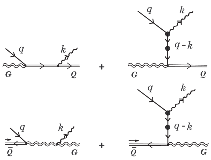
Figure 3: The scattering process of a soft fermion excitation by a hard parton such that statistics both hard and soft excitations are changed.

Both external soft legs lie on mass shell. In the case being considered one of soft external legs (quark leg, in this instance) is virtual and coupled with a static color center. In equation (4.5) this center is simulated by factors $|\,^{\ast}\!\Delta_{\pm}(q)|^{\,2}_{\,q_{0}=0}$. Thus the factorization of elastic part of the process under consideration from inelastic one takes place.

Let us determine expression for trace (4.5) in the high-frequency and small-angle approximations. The ‘elastic’ factors $|\,^{\ast}\!\Delta_{\pm}(q)|^{\,2}_{\,q_{0}=0}$ are most simply approximated. By using an explicit form for the scalar propagators (A.2), (A.3) it is not difficult to obtain

$$\lim\limits_{q_{0}\rightarrow 0}\,^{\ast}\!\Delta_{\pm}(q_{0},{\bf q})=\pm\,\frac{|{\bf q}|}{\,{\bf q}^{2}+\omega_{0}^{2}\,(1\mp i\pi/2)}\,.$$

Further, taking into account $\omega_{\bf k}^{t}-{\bf v}_{1}\cdot{\bf k}\simeq({\bf k}^{2}_{\perp}+m_{g}^{2}+x^{2}M^{2})/2\omega\equiv l^{-1}_{f}$, we have

$${\bf q}^{2}={\bf q}_{\perp}^{2}+q^{2}_{\|}\simeq{\bf q}_{\perp}^{2}+l^{-2}_{f}.$$

Here, $l_{f}$ and $m_{g}^{2}=(3\,g^{2}\!/2)\{(N_{c}+n_{f}/2)(T^{\,2}/9)+n_{f}(\mu^{2}/6\pi^{2})\}$ are the finite formation length for soft gluon radiation and the (squared) induced gluon mass, accordingly. Since we have restricted ourselves only to massless hard particles, in the subsequent discussion we will regularly neglect by possible mass terms of the type $x^{2}M^{2},\;x\equiv\omega/E_{1}$. Under the condition ${\bf q}_{\perp}^{2}\gg l^{-2}_{f}$ one puts the final touches to approximation of the ‘elastic’ factors

$$|\,^{\ast}\!\Delta_{\pm}(0,{\bf q})|^{\,2}\simeq\frac{{\bf q}_{\perp}^{2}}{\left({\bf q}^{2}_{\perp}+\omega_{0}^{2}\right)^{\,2}+\biggl{(}\displaystyle\frac{\omega_{0}^{2}\pi}{2}\biggr{)}^{\!\!2}}\,.$$ (4.7)

As the next step we will consider approximation of the coefficient functions $\acute{\rho}_{\pm}$ and ${\rho}_{\pm}$ in (4.5). Let us approximate the second term on the right-hand side of (4.6). Simple reasoning leads to

$${\bf v}_{1}\cdot\hat{\bf q}\equiv\frac{{\bf v}_{1}\cdot{\bf q}}{|\,{\bf q}|}=-\,\frac{(\omega_{\bf k}^{t}-{\bf v}_{1}\cdot{\bf k})}{|{\bf q}|}\simeq-\frac{1}{|\,{\bf q}_{\perp}|}\,l_{f}^{-1}.$$ (4.8)

For the third term we have a chain of equalities:

$$\hat{\bf q}\cdot\hat{\bf l}\,=\,\frac{{\bf q}_{\perp}\!\cdot({\bf q}-{\bf k})_{\perp}\!+q_{\|}(q-k)_{\|}}{|{\bf q}||\,{\bf q}-{\bf k}|}\,\simeq\,\frac{{\bf q}_{\perp}\!\cdot({\bf q}-{\bf k})_{\perp}\!+\omega\,l_{f}^{-1}}{|{\bf q}||\,{\bf q}-{\bf k}|},\quad\omega\equiv k_{\|}.$$

Taking into account the approximations

$$\frac{1}{|\,{\bf q}-{\bf k}|}\,\simeq\,\frac{1}{k_{\|}}-\frac{1}{k_{\|}^{3}}\,\left\{k_{\|}\,l_{f}^{-1}+({\bf q}-{\bf k})^{2}_{\perp}\right\},\quad\frac{1}{|{\bf q}|}\,\simeq\,\frac{1}{|\,{\bf q}_{\perp}|}\,\Biggl{(}1-\frac{l_{f}^{-2}}{2\,{\bf q}_{\perp}^{2}}\Biggr{)},$$ (4.9)

we finally obtain

$$\hat{\bf q}\cdot\hat{\bf l}\;\simeq\;\frac{1}{|\,{\bf q}_{\perp}|}\,\Biggl{\{}\frac{1}{\,l_{f}}\,+\,\frac{{\bf q}_{\perp}\!\cdot({\bf q}-{\bf k})_{\perp}}{\omega}\Biggr{\}}.$$ (4.10)

Eventially, for the last term on the right-hand side of Eq. (4.6) it is not difficult to derive

$${\bf v}_{1}\cdot\hat{\bf l}=-\,\frac{\omega_{\bf k}^{t}}{|\,{\bf l}|}\,\simeq\,-1+\frac{({\bf q}-{\bf k})^{2}_{\perp}}{2\,\omega^{2}}\,.$$

Considering all the above-stated approximations, we find that the $\acute{\rho}_{\pm}$ and ${\rho}_{\pm}$ coefficient functions are approximated at leading order by the following expressions:

$$\acute{\rho}_{+}\simeq{\rho}_{+}\simeq 2,\quad\acute{\rho}_{-}\simeq-{\rho}_{-}\simeq-\,\frac{{\bf q}_{\perp}\!\cdot({\bf q}-{\bf k})_{\perp}}{\omega|\,{\bf q}_{\perp}|}\,.$$ (4.11)

It is evident that the $\acute{\rho}_{-}$ and ${\rho}_{-}$ functions are suppressed in comparison with the $\acute{\rho}_{+}$ and ${\rho}_{+}$ ones.

Let us now turn to an approximation of scalar amplitudes (4.4). For the first term here we can use conventional expression for the approximation in question

$$\frac{{\bf e}\cdot{\bf v}_{1}}{\omega_{\bf k}^{t}-{\bf v}_{1}\cdot{\bf k}}\,\simeq\,-\,2\,\frac{{\bf e}_{\perp}\cdot{\bf k}_{\perp}}{{\bf k}_{\perp}^{2}+m_{g}^{2}}\,.$$ (4.12)

In the second term we will consider, at first, approximations of the scalar propagators $\,{}^{\ast}\!\Delta_{\pm}(l)$. We make use their explicit expressions given in Appendix A. In the denominator of the $\,{}^{\ast}\!\Delta_{-}(l)$ propagator the term $\delta\Sigma_{-}(l)$ can be dropped and $|\,{\bf l}|$ should be replaced by $\omega$. As a result to leading order we have

$$\,{}^{\ast}\!\Delta_{-}(\omega_{\bf k}^{t},{\bf l})\,\simeq\,-\frac{1}{\,2\omega}\,.$$

Furthermore, for the soft-quark self-energy $\delta\Sigma_{+}(l)$ one has approximation

$$\delta\Sigma_{+}(\omega_{\bf k}^{t},{\bf l})\,\simeq\,\frac{\omega_{0}^{2}}{|\,{\bf l}|}\,\Biggl{(}1+\frac{({\bf q}-{\bf k})^{2}_{\perp}}{4\,\omega^{2}}\,\Biggl{\{}\ln\frac{4\omega^{2}}{({\bf q}-{\bf k})^{2}_{\perp}}-i\pi\!\Biggr{\}}\Biggr{)}.$$

Under the condition

$$\epsilon\ln\epsilon\ll 1,\quad\epsilon\equiv({\bf q}-{\bf k})^{2}_{\perp}/\omega^{2}$$

the preceding expression can be simplified having put $\delta\Sigma_{+}(\omega_{\bf k}^{t},{\bf l})\simeq\omega_{0}^{2}/|\,{\bf l}|$. Hence it immediately follows that

$$\,{}^{\ast}\!\Delta_{+}(\omega_{\bf k}^{t},{\bf l})\,\simeq\,\frac{2\omega}{({\bf q}-{\bf k})^{2}_{\perp}+m_{q}^{2}}\,,$$ (4.13)

where $m_{q}^{2}=2\omega^{2}_{0}$ is the induced quark mass squared. It is evident that the propagator $\,{}^{\ast}\!\Delta_{-}(l)$ is suppressed with respect to $\,{}^{\ast}\!\Delta_{+}(l)$.

Approximations of the vertex factors $\acute{{\it\Gamma}}_{\pm}^{\,i}{\rm e}^{i}(\hat{\bf k},\xi)$ and ${\it\Gamma}_{\pm}^{\,i}{\rm e}^{i}(\hat{\bf k},\xi)$ are more complicated and cumbersome (an explicit form of the vertex functions is given in Appendix A). Omitting tedious calculations we want at once to present the final result up to the next to leading order:

$$\acute{{\it\Gamma}}_{\pm}^{\,i}{\rm e}^{i}(\hat{\bf k},\xi)\,\simeq\,-\frac{{\rm e}_{\perp}\cdot{\bf q}_{\perp}}{|\,{\bf q}_{\perp}|}\,\mp\,\Biggl{[}\,1-\frac{1}{\,{\bf q}_{\perp}^{\,2}}\,\Bigl{(}{\bf q}_{\perp}\cdot({\bf q}-{\bf k})_{\perp}+\omega l_{f}^{-1}\Bigr{)}\Biggr{]},$$ (4.14)

$${\it\Gamma}_{\pm}^{\,i}{\rm e}^{i}(\hat{\bf k},\xi)\,\simeq\,+\,\frac{{\rm e}_{\perp}\cdot{\bf q}_{\perp}}{|\,{\bf q}_{\perp}|}\,\mp\,\Biggl{[}\,1-\frac{1}{\,{\bf q}_{\perp}^{\,2}}\,\Bigl{(}{\bf q}_{\perp}\cdot({\bf q}-{\bf k})_{\perp}+\omega l_{f}^{-1}\Bigr{)}\Biggr{]},\hskip 5.69046pt$$

Let us now return to initial expression (4.5). By using the above estimations one can show that terms containing the differences of the scalar amplitudes: $\acute{\cal M}_{+}^{t}\!-\!\acute{\cal M}_{-}^{t}$ and ${\cal M}_{+}^{t}\!-\!{\cal M}_{-}^{t}$ to leading order exactly cancel each other. Furthermore, by virtue of estimations (4.11), (4.13) and (4.14) we can neglect contributions of terms containing the scalar amplitudes $\acute{\cal M}_{-}^{t}$ and ${\cal M}_{-}^{t}$. Finally, we see the first term ${\bf e}\cdot{\bf v}_{1}/(\omega_{\bf k}^{t}-{\bf v}_{1}\cdot{\bf k})$ in the $\acute{\cal M}_{+}^{t}$ and ${\cal M}_{+}^{t}$ amplitudes in view of estimations (4.13), (4.14) and (4.12) to be suppressed in comparison with the second one by the factor $|\,{\bf q}_{\perp}|/\omega$. To sum up, at leading order trace (4.5) is approximated by the following simple expression:

$${\rm Sp}\!\left[\,(v_{1}\cdot\gamma)A_{\|}\,\gamma^{0}(\gamma^{0}A^{\dagger}_{\|}\gamma^{0})\right]$$ (4.15)

$$\simeq\,16\,\omega^{2}\frac{1}{\Bigl{(}{\bf q}^{2}_{\perp}+\omega_{0}^{2}\Bigr{)}^{2}+\biggl{(}\displaystyle\frac{\omega_{0}^{2}\pi}{2}\biggr{)}^{\!2}}\;\frac{({\bf e}_{\perp}\cdot{\bf q}_{\perp})^{2}}{\Bigl{[}({\bf q}-{\bf k})^{2}_{\perp}+m_{q}^{2}\Bigr{]}^{2}}\,.$$

Let us recall now about existence of ‘transverse’ part of the total amplitude $A$, which defined by the expression

$$A_{\perp}=-\Bigl{[}\,h_{+}(\hat{\bf l})\,(\!\,^{\ast}\!\Delta_{+}(l))^{\ast}+h_{-}(\hat{\bf l})\,(\!\,^{\ast}\!\Delta_{-}(l))^{\ast}\,\Bigr{]}({\bf n}\cdot{\bf\gamma})({\it\Gamma}_{1\perp}^{\,i}{\rm e}^{i})$$

$$\times\,\Bigl{[}\,h_{+}(\hat{\bf q})\,^{\ast}\!\Delta_{+}(q)+h_{-}(\hat{\bf q})\,^{\ast}\!\Delta_{-}(q)\Bigr{]}.\hskip 28.45274pt$$

We substitute the $A_{\perp}$ amplitude into equation (4.1). Somewhat bulky calculations of the trace lead to expression which is quite similar one (4.5), namely

$${\rm Sp}\!\left[\,(v_{1}\cdot\gamma)A_{\perp}\,\gamma^{0}(\gamma^{0}A^{\dagger}_{\perp}\gamma^{0})\right]={\bf n}^{2}\Bigl{|}{\it\Gamma}_{1\perp}^{\,i}{\rm e}^{i}\Bigr{|}^{\,2}\,|\,^{\ast}\!\Delta_{+}(q)|^{\,2}\,$$ (4.16)

$$\times\,\biggl{\{}{\rho}_{+}({\bf v}_{1};\hat{\bf q},\hat{\bf l})\,|\,^{\ast}\!\Delta_{+}(l)|^{\,2}+{\rho}_{-}({\bf v}_{1};\hat{\bf q},\hat{\bf l})\,|\,^{\ast}\!\Delta_{-}(l)|^{\,2}-\frac{{\bf v}_{1}\cdot({\bf n}\times{\bf l})}{|{\bf q}|\;{\bf l}^{2}}\,\left|\,{}^{\ast}\!\Delta_{+}(l)-\,^{\ast}\!\Delta_{-}(l)\right|^{\,2}\biggr{\}}$$

$$+\,\Bigl{(}\,^{\ast}\!\Delta_{+}(q)\rightarrow\,^{\ast}\!\Delta_{-}(q),\;{\rho}_{\pm}\rightarrow\acute{\rho}_{\pm}\Bigr{)}.$$

In above we do not know an approximation of the vertex factor ${\it\Gamma}_{1\perp}^{\,i}{\rm e}^{i}$ only. Making use the definition of the scalar ‘transverse’ vertex ${\it\Gamma}_{1\perp}^{\,i}$ (A.6), we write out initial expression for subsequent analysis

$${\bf n}^{2}\,\Bigl{|}{\it\Gamma}_{1\perp}^{\,i}{\rm e}^{i}\Bigr{|}^{\,2}=\,\frac{({\bf n}\cdot{\bf e})^{2}}{{\bf n}^{2}}\,,$$ (4.17)

where we immediately can write approximation for the denominator

$${\bf n}^{2}=({\bf l}\times{\bf q})^{2}={\bf q}^{2}{\bf l}^{2}\Bigl{[}1-(\hat{\bf q}\cdot\hat{\bf l})^{2}\Bigr{]}\simeq{\bf q}^{2}_{\perp}\omega^{2}.$$ (4.18)

The scalar product in the numerator of Eq. (4.17) can be presented as decomposition into longitudinal and transverse parts

$${\bf n}\cdot{\bf e}=n_{\|}{\rm e}_{\|}+{\bf n}_{\perp}\cdot{\bf e}_{\perp}.$$ (4.19)

Here, we have ${\rm e}_{\|}\simeq-({\bf k}_{\perp}\cdot{\bf e}_{\perp})/\omega$ by virtue of the condition of transversity. On the other hand the vector ${\bf n}$ can be written as

$${\bf n}=({\bf l}\times{\bf q})=({\bf l}_{\perp}+{\bf v}_{1}l_{\|})\times({\bf q}_{\perp}+{\bf v}_{1}q_{\|})$$

$$=({\bf l}_{\perp}\times{\bf q}_{\perp})+\Big{\{}({\bf v}_{1}\times{\bf q}_{\perp})l_{\|}+({\bf l}_{\perp}\times{\bf v}_{1})q_{\|}\Bigr{\}}\equiv n_{\|}{\bf v}_{1}+{\bf n}_{\perp}.$$

Hence it is not difficult to find an explicit form of the components $n_{\|}$ and ${\bf n}_{\perp}$. Making use the expressions obtained and approximations $q_{\|}\simeq-l_{f}^{-1}$, $l_{\|}\simeq-\omega-l_{f}^{-1}$, we find instead of Eq. (4.19)

$${\bf n}\cdot{\bf e}\,\simeq\,\omega\,{\bf v}_{1}\cdot({\bf e}_{\perp}\!\times{\bf q}_{\perp})-\!\Biggl{\{}\frac{1}{\,\omega}\,({\bf e}_{\perp}\cdot{\bf k}_{\perp})({\bf v}_{1}\cdot({\bf l}_{\perp}\!\times{\bf q}_{\perp}))-\frac{1}{\,l_{f}}\,({\bf v}_{1}\cdot({\bf e}_{\perp}\!\times{\bf k}_{\perp}))\Biggr{\}}.$$ (4.20)

The first term on the right-hand side here is the leading one. Substituting approximations (4.18) and (4.20) into Eq. (4.17), we derive the desired approximation of the vertex factor

$${\bf n}^{2}\,\Bigl{|}{\it\Gamma}_{1\perp}^{\,i}{\rm e}^{i}\Bigr{|}^{\,2}\simeq\,\frac{({\bf e}_{\perp}\!\times{\bf q}_{\perp})^{2}}{{\bf q}^{2}_{\perp}}\,.$$

Here we have taken into consideration that $({\bf v}_{1}\cdot({\bf e}_{\perp}\!\times{\bf q}_{\perp}))^{2}=({\bf e}_{\perp}\!\times{\bf q}_{\perp})^{2}$ at ${\bf v}_{1}^{2}=1$. As in the case of approximation of the trace with the ‘longitudinal’ amplitude $A_{\|}$, in expression (4.16) the terms with the coefficient functions $\rho_{+}$ and $\acute{\rho}_{+}$ are the leading ones. Setting $\rho_{+}\simeq\acute{\rho}_{+}=2$ and making use of the approximations for quark scalar propagators (4.7), (4.13) and the vertex factor (the preceding expression), we derive final form of approximation for the trace with the ‘transverse’ amplitude $A_{\perp}$:

$${\rm Sp}\!\left[\,(v_{1}\cdot\gamma)A_{\perp}\,\gamma^{0}(\gamma^{0}A^{\dagger}_{\perp}\gamma^{0})\right]$$ (4.21)

$$\simeq\,16\,\omega^{2}\frac{1}{\Bigl{(}{\bf q}^{2}_{\perp}+\omega_{0}^{2}\Bigr{)}^{2}+\biggl{(}\displaystyle\frac{\omega_{0}^{2}\pi}{2}\biggr{)}^{\!2}}\;\frac{({\bf e}_{\perp}\times{\bf q}_{\perp})^{2}}{\Bigl{[}({\bf q}-{\bf k})^{2}_{\perp}+m_{q}^{2}\Bigr{]}^{2}}\,.$$

Let us consider also the remaining interference contributions between the amplitudes $A_{\|}$ and $A_{\perp}$. Omitting calculations, we give the final expression for their approximation

$${\rm Sp}\!\left[\,(v_{1}\cdot\gamma)A_{\|}\,\gamma^{0}(\gamma^{0}A^{\dagger}_{\perp}\gamma^{0})\right]+{\rm Sp}\!\left[\,(v_{1}\cdot\gamma)A_{\perp}\,\gamma^{0}(\gamma^{0}A^{\dagger}_{\|}\gamma^{0})\right]$$

$$\simeq\,4\,\frac{({\rm e}_{\perp}\cdot{\bf q}_{\perp})}{\omega^{2}}\,\frac{1}{\!\Bigl{(}{\bf q}^{2}_{\perp}+\omega_{0}^{2}\Bigr{)}^{2}+\biggl{(}\displaystyle\frac{\omega_{0}^{2}\pi}{2}\biggr{)}^{\!2}\,}\;\,\frac{({\bf v}_{1}\cdot({\bf l}_{\perp}\times{\bf q}_{\perp}))({\bf v}_{1}\cdot({\bf e}_{\perp}\times{\bf q}_{\perp}))}{\Bigl{[}({\bf q}-{\bf k})^{2}_{\perp}+m_{q}^{2}\Bigr{]}}\,.$$

From this estimation we see the interference contribution to the scattering probability to be suppressed in comparison with direct contributions (4.15) and (4.21).

Now we consider in the expression for soft-gluon radiation intensity (3.6) the second term in braces. Let us change the integration variable: ${\bf q}\rightarrow-{\bf q}$. In the static limit we are to analyze the following additional contribution:

$$\int\!d{\bf q}_{\perp}dq_{\|}\left|\,\bar{\chi}_{1}\!\left({\rm e}^{i}(\hat{\bf k},\zeta){\cal K}^{i}({\bf v}_{1},0|\,-k,q)\right)\!\chi_{2}\right|^{\,2}_{\,k_{0}=\omega^{t}_{\bf k},\;q_{0}=0}\delta(\omega^{t}_{\bf k}-{\bf v}_{1}\cdot{\bf k}+q_{\|}).$$ (4.22)

Instead of amplitude (4.2) now we will have

$$\left.A={\rm e}^{i}(\hat{\bf k},\xi){\cal K}^{i}({\bf v}_{1},0|\,-k,q)\right|_{\,q_{0}=0,\;q_{\|}=-\,(\omega_{\bf k}^{t}-{\bf v}_{1}\cdot{\bf k})}$$

$$\left.=\Biggl{\{}\,-\frac{({\bf e}(\hat{\bf k},\xi)\cdot{\bf v}_{1})}{\omega_{\bf k}^{t}-{\bf v}_{1}\cdot{\bf k}}\,+\,^{\ast}\!S(q-k)\,\Gamma^{i}(-k;k-q,q)\,{\rm e}^{i}(\hat{\bf k},\xi)\Biggr{\}}\,^{\ast}\!S(-q)\right|_{\,q_{0}=0,\;q_{\|}=-\,(\omega_{\bf k}^{t}-{\bf v}_{1}\cdot{\bf k})}\,.$$

The sign of the first term is changed. However, this term is subleading and therefore it gives no contribution. In the second term the signs of arguments for all of the functions (besides the polarization vector ${\bf e}(\hat{\bf k},\xi)$) change. From an explicit form of approximations (4.15) and (4.21) we see these expressions at leading order to be even functions of variables ${\bf q}_{\perp}$ and $({\bf q}_{\perp}-{\bf k})_{\perp}$. Therefore the change of signs of arguments in starting formulae (4.5) and (4.16) does not influence the result of approximations. Consequently, to allow for (4.22) it is sufficient to multiply (4.5) and (4.16) by the factor $2$.

As already mentioned at the beginning of this section the expression for soft gluon radiation intensity (3.6) in the static limit defines the radiation energy losses of a hard parton 1. Summing approximations (4.15) and (4.21) and multiplying them by the factor $1/16E_{1}E_{2}$, we derive from Eq. (3.6) (taking into account (3.7)) the desired expression for energy losses

$$\Biggl{(}-\frac{dE_{1}}{dx}\Biggr{)}^{\!t}=2\,\frac{2}{E_{1}}\,\Biggl{(}\frac{{\alpha}_{s}^{3}}{\pi^{2}}\Biggr{)}\Biggl{(}\sum\limits_{\;\zeta=Q,\,\bar{Q}}\!C_{\theta\theta}^{(1;\zeta)}\!\int\!|\,{\bf p}_{2}|\left[\,f_{{\bf p}_{2}}^{(\zeta)}+f_{{\bf p}_{2}}^{(G)}\right]\frac{d|\,{\bf p}_{2}|}{2\pi^{2}}\,\Biggr{)}\!\int\!\omega^{2}d\omega$$ (4.23)

$$\times\!\int\!d{\bf k}_{\perp}\!\int\!d{\bf q}_{\perp}\frac{{\bf q}_{\perp}^{2}}{\Bigl{(}{\bf q}^{2}_{\perp}+\omega_{0}^{2}\Bigr{)}^{2}+\biggl{(}\displaystyle\frac{\omega_{0}^{2}\pi}{2}\biggr{)}^{\!2}}\;\frac{1}{\Bigl{[}({\bf q}-{\bf k})^{2}_{\perp}+m_{q}^{2}\Bigr{]}^{2}}\,.$$

In deriving this expression we have taken into account

$$({\bf e}_{\perp}\cdot{\bf q}_{\perp})^{2}+({\bf e}_{\perp}\!\times{\bf q}_{\perp})^{2}={\bf e}_{\perp}^{2}{\bf q}_{\perp}^{2},\quad\sum\limits_{\xi=1,\,2}\!{\bf e}_{\perp}^{2}(\hat{\bf k},\xi)=2$$

and the approximations ${\rm Z}_{t}({\bf k})\simeq 1$, $\omega_{\bf k}^{t}\simeq k_{\|}\equiv\omega$, and $E_{2}\simeq|{\bf p}_{2}|\,$. The overall factor $2$ takes into consideration the contribution from term (4.22). The integrals over $d{\bf q}_{\perp}$ and $d{\bf k}_{\perp}$ are finite. If the kinematic bounds are ignored, then by introducing the polar coordinates it is not difficult to show that the integration over $d{\bf k}_{\perp}d{\bf q}_{\perp}$ can be presented as follows:

$$-\pi^{2}\!\int\limits_{0}^{\infty}\!d{\bf k}_{\perp}^{2}\,\frac{\partial}{\partial m_{q}^{2}}\int\limits_{0}^{\infty}\!\frac{{\bf q}_{\perp}^{2}d{\bf q}_{\perp}^{2}}{\Bigl{(}{\bf q}^{2}_{\perp}+\omega_{0}^{2}\Bigr{)}^{2}+\biggl{(}\displaystyle\frac{\omega_{0}^{2}\pi}{2}\biggr{)}^{\!2}}\;\frac{1}{\sqrt{{\bf q}^{4}_{\perp}-2({\bf k}^{2}_{\perp}-m_{q}^{2})\,{\bf q}^{2}_{\perp}+({\bf k}^{2}_{\perp}+m_{q}^{2})^{2}}}\,.$$

The integral under the derivative sign is exactly calculated and expressed in terms of the logarithm or arctangent functions. The final expressions are rather cumbersome and for this reason we does not present them here.

5 Approximation of static color center for soft quark bremsstrahlung

Let us turn to analysis of formula for quark radiation intensity (3.10) within the framework of the static color center approximation. At the beginning we consider the first term on the right-hand side of Eq. (3.10). For the sake of simplicity we restrict ourselves only to bremsstrahlung of soft quark normal mode, i.e. according to (3.11) we set in (3.10)

$${\rm Im}\,^{\ast}\!\Delta_{+}(q)\simeq-\,\pi\,{\rm Z}_{+}({\bf q})\,\delta(q^{0}-\omega_{\bf q}^{+}).$$

As well as in the previous case, as a first step, consider the integral over the momentum transfer ${\bf q}_{1}$:

$$\sum\limits_{\lambda\,=\,\pm}\!\int\!d{\bf q}_{1\perp}dq_{1\|}\left|\,\bar{u}(\hat{\bf q},\lambda){\cal K}({\bf v}_{1},0;\chi_{1},\chi_{2}|\,q,-q_{1})\right|^{\,2}_{\,q_{0}=\omega^{+}_{\bf q},\;q_{1}^{0}=0}\delta(\omega^{+}_{\bf q}-{\bf v}_{1}\cdot{\bf q}+q_{\|}).$$

Recall that in the static approximation it is necessary not only to set ${\bf v}_{1}=0$, but neglect all the contributions proportional to $(\bar{u}(\hat{\bf q},\lambda)\chi_{2})$ as well. In this case it results in that in the ${\cal K}_{\alpha}$ function (2.10) the second term should be omitted. For completely unpolarized states of hard partons 1 and 2 the module squared in the integrand of the above equation can be presented in the form similar to (4.1)

$$\sum\limits_{\lambda\,=\,\pm}\!\left|\,\bar{u}(\hat{\bf q},\lambda){\cal K}({\bf v}_{1},0;\chi_{1},\chi_{2}|\,q,-q_{1})\right|^{\,2}$$ (5.1)

$$=\frac{1}{4E_{2}}\Biggl{\{}|\,^{\ast}\!\Delta_{+}(q_{1})|^{\,2}\,{\rm Sp}\!\left[\,{\cal M}h_{+}(\hat{\bf q}_{1})(\gamma^{0}{\cal M}^{\dagger}\gamma^{0})h_{+}(\hat{\bf q})\right]$$

$$\hskip 42.67912pt+\,|\,^{\ast}\!\Delta_{-}(q_{1})|^{\,2}\,{\rm Sp}\!\left[\,{\cal M}h_{-}(\hat{\bf q}_{1})(\gamma^{0}{\cal M}^{\dagger}\gamma^{0})h_{+}(\hat{\bf q})\right]\Biggr{\}},$$

where we have introduced (matrix) amplitude

$${\cal M}\equiv{\cal M}(q,q_{1})=\frac{\alpha}{4E_{1}}\,\frac{(v_{1}\cdot\gamma)}{(v_{1}\cdot q_{1})}\,-\,^{\ast}\Gamma^{(Q)\mu}(q-q_{1};q_{1},-q)\!\,^{\ast}{\cal D}_{\mu\nu}(q-q_{1})v_{1}^{\nu}.$$

In Appendix B the details of calculations of the traces in (5.1) are given. This leads to the following expression for the first trace:

$${\rm Sp}\!\left[\,{\cal M}h_{+}(\hat{\bf q}_{1})(\gamma^{0}{\cal M}^{\dagger}\gamma^{0})h_{+}(\hat{\bf q})\right]=\frac{1}{4}\;(1+\,\hat{\bf q}\cdot\hat{\bf q}_{1})$$ (5.2)

$$\times\Biggl{|}\Bigl{\{}{\cal M}_{l}({\bf p}_{1}|\,{\bf q},{\bf q}_{1})-{\cal M}_{l}^{\ast}({\bf p}_{1}|\,{\bf q}_{1},{\bf q})\Bigr{\}}({\bf v}_{1}\cdot{\bf l})+\Bigl{\{}{\cal M}_{t}({\bf p}_{1}|\,{\bf q},{\bf q}_{1})+{\cal M}_{t}^{\ast}({\bf p}_{1}|\,{\bf q}_{1},{\bf q})\Bigr{\}}\frac{({\bf v}_{1}\cdot({\bf n}\times{\bf l}))}{{\bf n}^{2}\,{\bf l}^{2}}\Biggr{|}^{\,2}$$

$$+\,\frac{1}{4}\;(1-\,\hat{\bf q}\cdot\hat{\bf q}_{1})\Bigl{|}\,{\cal M}_{\!1t}({\bf p}_{1}|\,{\bf q},{\bf q}_{1})+{\cal M}_{\!1t}^{\ast}({\bf p}_{1}|\,{\bf q}_{1},{\bf q})\Bigr{|}^{\,2}\,\frac{({\bf v}_{1}\cdot{\bf n})^{2}}{{\bf n}^{2}}.$$

Here, the scalar amplitudes ${\cal M}_{l},\,{\cal M}_{t}$ and ${\cal M}_{1t}$ have the following structure:

$${\cal M}_{l}({\bf p}_{1}|\,{\bf q},{\bf q}_{1})=\frac{\alpha}{2E_{1}}\,\frac{1}{(v_{1}\cdot q_{1})}\,\frac{1}{|{\bf l}|}\,\Biggl{(}\frac{1}{2}\,\frac{|{\bf l}|}{l^{0}}+\frac{|{\bf q}_{1}|}{|{\bf l}|}\Biggr{)}-\Biggl{(}\frac{l^{2}}{l_{0}^{2}\,{\bf l}^{2}}\Biggr{)}\Bigl{(}\,^{\ast}\!\acute{{\it\Gamma}}_{+}^{\,i}(l;q_{1},-q)\,l^{i}\,\Bigr{)}\,^{\ast}\!\Delta^{l}(l),$$

$${\cal M}_{t}({\bf p}_{1}|\,{\bf q},{\bf q}_{1})=\frac{\alpha}{2E_{1}}\,\frac{1}{(v_{1}\cdot q_{1})}\,|{\bf q}_{1}|({\bf l}\cdot{\bf q})\,-\Bigl{(}\,^{\ast}\!\acute{{\it\Gamma}}_{+}^{\,i}(l;q_{1},-q)({\bf n}\times{\bf l})^{i}\,\Bigr{)}\,^{\ast}\!\Delta^{t}(l),\hskip 19.91684pt$$ (5.3)

$${\cal M}_{\!1t}({\bf p}_{1}|\,{\bf q},{\bf q}_{1})=\frac{\alpha}{4E_{1}}\,\,\frac{1}{(v_{1}\cdot q_{1})}\,-\Bigl{(}\,^{\ast}\!{\it\Gamma}_{1\perp}^{\,i}(l;q_{1},-q)\,n^{i}\,\Bigr{)}\,^{\ast}\!\Delta^{t}(l),$$

where now

$$l\equiv q-q_{1},\quad{\bf n}\equiv({\bf q}_{1}\times{\bf q}).$$

The second trace in (5.1) is derived from the first one by the replacements: $(1\pm\,\hat{\bf q}\cdot\hat{\bf q}_{1})\rightarrow(1\mp\,\hat{\bf q}\cdot\hat{\bf q}_{1})$ and $\,{}^{\ast}\!\acute{{\it\Gamma}}_{+}^{\,i}(l;q_{1},-q)\rightarrow\,^{\ast}\!\acute{{\it\Gamma}}_{-}^{\,i}(l;q_{1},-q)$.

Now we consider approximation of expression (5.1). By virtue of analysis in the preceding section we can set at once

$$|\,^{\ast}\!\Delta_{\pm}(0,{\bf q}_{1})|^{\,2}\simeq\frac{{\bf q}_{1\perp}^{2}}{\,\left({\bf q}^{2}_{1\perp}+\omega_{0}^{2}\right)^{\,2}+\biggl{(}\displaystyle\frac{\omega_{0}^{2}\pi}{2}\biggr{)}^{\!\!2}}\,.$$

In fact, here one also observes factorization of scattering probability (5.1) into a product of ’elastic’ and ’inelastic’ parts. In Paper II we have obtained the probability of the elastic scattering of soft-quark excitations off hard test parton ${\it w}_{\,q\rightarrow q}^{(\zeta)(f,\,f_{1})}({\bf p}|\,{\bf q};{\bf q}_{1})$ (Eqs. (II.8.22), (II.8.21) and Figs. (II.1), (II.3)). Up to kinematic and color factors this scattering probability for normal modes, i.e. for $f=f_{1}=+$, exactly coincides with expressions (5.2), (5.3). The only essential difference between these two cases lies in the fact that in the last case one of external soft quark lines is virtual and connected with a static color center simulated by $|\,^{\ast}\!\Delta_{\pm}(0,{\bf q}_{1})|^{\,2}$.

Further, let us consider approximation of the first term on the right-hand side of Eq. (5.2). Preliminary analysis shown the contribution containing difference of scalar ’longitudinal’ amplitudes ${\cal M}_{l}({\bf p}_{1}|\,{\bf q},{\bf q}_{1})-{\cal M}_{l}^{\ast}({\bf p}_{1}|\,{\bf q}_{1},{\bf q})$ to be subleading in comparison with the contribution containing the sum of scalar ‘transverse’ amplitudes. Therefore we shall concentrate our attention on an approximation of the second contribution in the term under consideration, namely

$$\frac{({\bf v}_{1}\cdot({\bf n}\times{\bf l}))}{{\bf n}^{2}\,{\bf l}^{2}}\,\Bigl{\{}{\cal M}_{t}({\bf p}_{1}|\,{\bf q},{\bf q}_{1})+{\cal M}_{t}^{\ast}({\bf p}_{1}|\,{\bf q}_{1},{\bf q})\Bigr{\}}.$$ (5.4)

First of all one approximates here the kinematic factor. We can use some of expressions for approximations obtained in the previous section with relevant replacements. So for the ${\bf n}^{2}$ by virtue of (4.18) we have: ${\bf n}^{2}\simeq\omega^{2}{\bf q}^{2}_{1\perp}$, where now $\omega\equiv q_{\|}$. Furthermore, the triple product ${\bf v}_{1}\cdot({\bf n}\times{\bf l})$ can be written as

$$\omega_{\bf q}^{+}({\bf l}\cdot{\bf q})-{\bf l}^{2}({\bf v}_{1}\cdot{\bf q}).$$

For the normal quark mode $\omega_{\bf q}^{+}$ in the small-angle approximation we derive

$$\omega_{\bf q}^{+}\simeq\sqrt{{\bf q}^{2}+m_{q}^{2}}\simeq q_{\|}+\frac{{\bf q}^{2}_{\perp}+m_{q}^{2}}{2\omega}\,.$$ (5.5)

Further, we have

$$({\bf l}\,\cdot{\bf q})\,\simeq\,q_{\|}^{2}\,+\,[\,({\bf l}_{\perp}\cdot{\bf q}_{\perp})+({\bf q}^{2}_{\perp}+m_{q}^{2})/2\,],$$ (5.6)

$$\hskip 14.22636pt({\bf v}_{1}\cdot{\bf q})\,\simeq\,q_{\|}\,+\,(\,{\bf q}^{2}_{\perp}+{\bf l}^{2}_{\perp}+m_{q}^{2})/q_{\|},\quad{\bf l}^{2}\simeq q_{\|}^{2}.$$

In view of the above mentioned one obtains the desired approximation of the kinematic factor

$$\frac{{\bf v}_{1}\cdot({\bf n}\times{\bf l})}{{\bf n}^{2}\,{\bf l}^{2}}\,\simeq\,\frac{({\bf q}_{1\perp}\cdot{\bf l}_{\perp})}{\omega^{3}\,{\bf q}^{2}_{1\perp}}\,.$$ (5.7)

Let us consider the terms in the sum ${\cal M}_{t}+{\cal M}_{t}^{\ast}$ containing no vertex functions. By virtue of definition (5.3) they are equal to

$$\frac{\alpha}{2E_{1}}\,\frac{1}{(v_{1}\cdot q_{1})}\,\Bigl{[}\,|{\bf q}_{1}|({\bf l}\cdot{\bf q})-|{\bf q}|({\bf l}\cdot{\bf q}_{1})\Bigr{]}.$$ (5.8)

By the conservation momentum-energy law and Eq. (5.5) for the denominator in (5.8) we have

$$\frac{1}{(v_{1}\cdot q_{1})}=\frac{1}{(v_{1}\cdot q)}\simeq\frac{2\omega}{{\bf q}_{\perp}^{2}+m_{q}^{2}}\,.$$

Up to the next-to-leading order the following approximations hold

$$|{\bf q}_{1}|\simeq|\,{\bf q}_{1\perp}\!|+\frac{1}{2|\,{\bf q}_{1\perp}\!|}\,\frac{({\bf q}_{\perp}^{2}+m_{q}^{2})^{2}}{(2\omega)^{2}}\,,\quad|{\bf q}|\simeq q_{\|}+\frac{{\bf q}_{\perp}^{2}}{2\omega}\,.$$

Making use of these expressions and (5.6) we find to leading order, instead of (5.8)

$$\frac{\alpha}{E_{1}}\;\frac{|\,{\bf q}_{1\perp}\!|}{{\bf q}_{\perp}^{2}+m_{q}^{2}}\,.$$ (5.9)

Now consider the terms with the vertex functions in the sum ${\cal M}_{t}+{\cal M}_{t}^{\ast}$. We neglect the HTL-correction to the bare two-quark – gluon vertex. By virtue of definition (5.3) we have initial expression

$$-\Bigl{[}\,\acute{{\it\Gamma}}_{+}^{\,i}(l;q_{1},-q)({\bf n}\times{\bf l})^{i}\,{}^{\ast}\!\Delta^{t}(l)\,+\acute{{\it\Gamma}}_{+}^{\,i}(-l;q,-q_{1})({\bf n}\times{\bf l})^{i}\,{}^{\ast}\!\Delta^{t}(-l)\Bigr{]}.$$ (5.10)

Let us consider approximation of the first term in (5.10). For convenience of the further references we write out here an explicit form of the contraction $\acute{{\it\Gamma}}_{+}^{\,i}(l;q_{1},-q)({\bf n}\times{\bf l})^{i}$:

$$\acute{{\it\Gamma}}_{+}^{\,i}(l;q_{1},-q)({\bf n}\times{\bf l})^{i}=-|\,{\bf q}_{1}|{\it\Gamma}_{\|}^{\,i}(l;q_{1},-q)({\bf n}\times{\bf l})^{i}\,-\frac{{\bf n}^{2}}{|\,{\bf q}|}\,\frac{1}{1+\hat{\bf q}\cdot\hat{\bf q}_{1}}{\it\Gamma}_{\perp}^{\,i}(l;q_{1},-q)({\bf n}\times{\bf l})^{i},$$ (5.11)

where

$${\it\Gamma}_{\|}^{\,i}(l;q_{1},-q)=\frac{q_{1}^{i}}{{\bf q}_{1}^{2}},\quad{\it\Gamma}_{\perp}^{\,i}(l;q_{1},-q)=\frac{({\bf n}\times{\bf q}_{1})^{i}}{{\bf n}^{2}{\bf q}_{1}^{2}},\quad{\bf n}={\bf q}_{1}\times{\bf q}.$$

Approximation of the first vertex factor on the right-hand side of Eq. (5.11) is

$${\it\Gamma}_{\|}^{\,i}(l;q_{1},-q)({\bf n}\times{\bf l})^{i}=\frac{1}{\,{\bf q}_{1}^{2}}\,[({\bf l}\cdot{\bf q}_{1})^{2}-{\bf q}_{1}^{2}{\bf l}^{2}]\simeq\frac{1}{\,{\bf q}_{1\perp}^{2}}\,(-{\bf q}_{1\perp}^{2}q_{\|}^{2})=-q_{\|}^{2}$$

and thus approximation of the first term reads

$$-|\,{\bf q}_{1}|\,{\it\Gamma}_{\|}^{\,i}(l;q_{1},-q)({\bf n}\times{\bf l})^{i}\simeq\omega^{2}|\,{\bf q}_{1\perp}|.$$

Further, we consider the second term in (5.11) which in view of definition of the ${\it\Gamma}_{\perp}^{\,i}$ function, equals

$$\frac{1}{|\,{\bf q}||\,{\bf q}_{1}|^{\,2}}\,\frac{({\bf n}\times{\bf l})\cdot({\bf n}\times{\bf q}_{1})}{1+\hat{\bf q}\cdot\hat{\bf q}_{1}}\simeq\frac{1}{\,q_{\|}\,{\bf q}_{1\perp}^{2}}\,{\bf n}^{2}({\bf l}\cdot{\bf q}_{1})\simeq\omega\left\{({\bf l}_{\perp}\cdot{\bf q}_{1\perp})-\frac{1}{2}\,({\bf q}^{2}_{\perp}+m_{q}^{2})\right\}.$$

The term is suppressed in comparison with the first one. To leading order we have approximation for scalar vertex (5.11)

$$\acute{{\it\Gamma}}_{+}^{\,i}(l;q_{1},-q)({\bf n}\times{\bf l})^{i}\,\simeq\,\omega^{2}|\,{\bf q}_{1\perp}|.$$ (5.12)

The second vertex factor in equation (5.10) is approximated in a similar way and results in the same estimate (5.12). Here, however, the main contribution goes from the second term proportional to ${\it\Gamma}_{\perp}^{\,i}(-l;,q,-q_{1})$. By using an approximation for the scalar transverse gluon propagator $\,{}^{\ast}\!\Delta^{t}(l)$

$$\,{}^{\ast}\!\Delta^{t}(l)\,\simeq\,-\frac{1}{({\bf q}-{\bf q}_{1})^{\,2}_{\perp}\!+m_{g}^{2}}\,,$$

we derive the final approximation of expression (5.10)

$$\frac{\omega^{2}|\,{\bf q}_{1\perp}|}{({\bf q}-{\bf q}_{1})^{\,2}_{\perp}\!+m_{g}^{2}}\,.$$

If one compares an approximation of the term without vertex function (5.9) with the above expression, it can be easily found that they are in the ratio $|\alpha|q_{\|}/E_{1}$. Thus under the condition when a high-energy parton 1 radiates very soft bremsstrahlung quark, i.e. when $|\alpha|\omega/E_{1}\ll 1$, the contribution of term (5.8) can be neglected. Taking into account the approximation of kinematic factor (5.7), we obtain finally the approximation for (5.4)

$$\frac{({\bf v}_{1}\cdot({\bf n}\times{\bf l}))}{{\bf n}^{2}\,{\bf l}^{2}}\,\Bigl{\{}{\cal M}_{t}({\bf p}_{1}|\,{\bf q},{\bf q}_{1})+{\cal M}_{t}^{\ast}({\bf p}_{1}|\,{\bf q}_{1},{\bf q})\Bigr{\}}\simeq 2\,\frac{1}{\omega|\,{\bf q}_{1\perp}|}\frac{({\bf q}_{1\perp}\cdot{\bf l}_{\perp})}{({\bf q}-{\bf q}_{1})^{\,2}_{\perp}\!+m_{g}^{2}}\,.$$

In Eq. (5.1) there exists the second similar contribution to scattering amplitude defined by the second term on the right-hand side. The accurate analysis of the leading term (5.10) (in which the following replacements should be performed $\acute{\Gamma}_{+}^{i}(l;q_{1},-q)\rightarrow\acute{\Gamma}_{-}^{i}(l;q_{1},-q),\,\acute{\Gamma}_{+}^{i}(-l;q,-q_{1})\rightarrow\acute{\Gamma}_{-}^{i}(-l;q,-q_{1})$) shows that instead of the sum of the scalar propagators $\!\,{}^{\ast}\!\Delta^{t}(l)+\!\,^{\ast}\!\Delta^{t}(-l)$, here we shall have their difference. This difference vanishes to leading order and therefore this contribution can be omitted.

We are coming now to an approximation of the ${\cal M}_{1t}$ amplitude in the second term of trace (5.2). On the strength of definitions of ${\cal M}_{1t}$ (5.3) and the vertex function $\Gamma_{1\perp}^{i}(l;q_{1},-q)=n_{i}/{\bf n}^{2}$, it is easily defined the approximation of this sum:

$${\cal M}_{1t}({\bf p}_{1}|\,{\bf q},{\bf q}_{1})+{\cal M}_{1t}^{\ast}({\bf p}_{1}|\,{\bf q}_{1},{\bf q})$$ (5.13)

$$=\frac{\alpha}{4E_{1}}\,\Biggl{(}\frac{1}{(v_{1}\cdot q_{1})}+\frac{1}{(v_{1}\cdot q)}\Biggr{)}-2\,\Bigl{(}\!\,^{\ast}\!\Delta^{t}(l)+\!\,^{\ast}\!\Delta^{t}(-l)\Bigr{)}$$

$$\simeq\frac{\alpha}{E_{1}}\,\frac{\omega}{{\bf q}_{\perp}^{\,2}\!+m_{q}^{2}}\,+\,2\,\frac{1}{({\bf q}-{\bf q}_{1})^{\,2}_{\perp}\!+m_{g}^{2}}\,.$$

Here we see again the first contribution to be suppressed in comparison with the second (vertex) contribution. Therefore to leading order this contribution can be neglected. Finally, the kinematic factor in the second term (5.2) can be approximated as follows:

$$\frac{({\bf v}_{1}\cdot{\bf n})^{2}}{{\bf n}^{2}}\simeq\frac{({\bf q}_{1\perp}\!\times{\bf l}_{\perp})^{2}}{\omega^{2}\,{\bf q}_{1\perp}^{2}}\,.$$

Let us recall an existence of the second term in initial equation (5.1). Here, we have the sum similar to (5.13). However, unlike the previous case with the sum of the amplitudes ${\cal M}_{t}+{\cal M}_{t}^{\ast}$ the sum in question is not suppressed in comparison with (5.13). The additional contribution from the second term in Eq. (5.1) simply doubles the approximation obtained (5.13).

Taking into account all the above-mentioned we write out the final expression for approximation of emission probability of soft bremsstrahlung quark within the framework of the static color center model

$$\sum\limits_{\lambda\,=\,\pm}\!\left|\,\bar{u}(\hat{\bf q},\lambda){\cal K}({\bf v}_{1},0;\chi_{1},\chi_{2}|\,q,-q_{1})\right|^{\,2}$$ (5.14)

$$\simeq\frac{1}{\,4\omega^{2}E_{2}}\,\frac{1}{\,\left({\bf q}^{2}_{1\perp}+\omega_{0}^{2}\right)^{\,2}+\biggl{(}\displaystyle\frac{\omega_{0}^{2}\pi}{2}\biggr{)}^{\!\!2}}\;\frac{\,({\bf q}_{1\perp}\!\cdot{\bf l}_{\perp})^{2}+2({\bf q}_{1\perp}\!\times{\bf l}_{\perp})^{2}}{\Bigl{[}\,({\bf q}-{\bf q}_{1})^{\,2}_{\perp}\!+m_{g}^{2}\Bigr{]}^{\,2}}\,.$$

Let us return to the expression for soft quark radiation intensity (3.10) and consider approximation of the second term with another coefficient function ${\cal K}_{\alpha}({\bf v}_{2},{\bf v}_{1};\chi_{2},\chi_{1}|\,q,-q+q_{1})$. This function in view of definition (2.10) in the approximation of static color center $({\bf v}_{2}=0,\,q_{1}^{0}=0)$ is defined by the following expression:

$$-\,\alpha\,\frac{\chi_{2\alpha}}{q^{0}}\;\left[\,\bar{\chi}_{2}\,^{\ast}S(q-q_{1})\chi_{1}\right]\,-\frac{\chi_{1\alpha}}{(v_{1}\cdot q_{1})}\,\!\,^{\ast}{\cal D}^{0\nu}(q_{1})v_{1\nu}$$ (5.15)

$$+\,\,^{\ast}{\cal D}^{0\nu}(q_{1})\!\,^{\ast}\Gamma_{\nu,\;\alpha\beta}^{(Q)}(q_{1};q-q_{1},-q)\,^{\ast}\!S_{\beta\beta^{\prime}}(q-q_{1})\chi_{1\beta^{\prime}}.$$

Here it is more convenient to choose $A_{0}$-gauge for the gluon propagator. In this gauge, we have:

$$\!\,{}^{\ast}{\cal D}^{0\nu}(q_{1})=\xi_{0}\,\frac{q_{1}^{\nu}}{q_{1}^{0}}\,,$$

where $\xi_{0}$ is the gauge-fixing parameter. Furthermore, in the last term of Eq. (5.15) by virtue of the effective Ward identity, the equality

$$\,{}^{\ast}\Gamma^{(Q)}_{\nu}(q_{1};q-q_{1},-q)q_{1}^{\nu}=\,^{\ast}\!S^{-1}(q-q_{1})-\!\,^{\ast}\!S^{-1}(q)$$

is valid. The term with $\!\,{}^{\ast}\!S^{-1}(q)$ vanishes on mass-shell of the plasma fermi-excitations. The remaining term with $\,{}^{\ast}S^{-1}(q-q_{1})$ gives a contribution equal to $\xi_{0}\chi_{1\alpha}/q_{0}$ which in accuracy is cancelled by the second term in (5.15). By this means we have exact initial expression

$$\bar{u}(\hat{\bf q},\lambda){\cal K}(0,{\bf v}_{1};\chi_{2},\chi_{1}|\,q,-q+q_{1})=-\,\alpha\,\frac{\,(\bar{u}(\hat{\bf q},\lambda)\chi_{2})}{q^{0}}\;\left[\,\bar{\chi}_{2}\,^{\ast}S(q-q_{1})\chi_{1}\right],$$

which shows that in the static limit the second term on the right-hand side of (3.8) is associated entirely with radiation from a target. Because of this, within the accuracy of the analysis, contribution of this term to radiation should be omitted.

Let us set in (3.10) ${\rm Im}\,^{\ast}\!\Delta_{+}(q)\simeq-\,\pi\,{\rm Z}_{+}({\bf q})\,\delta(q^{0}-\omega_{\bf q}^{+}),\,{\rm Z}_{+}({\bf q})\simeq 1$ and $\omega_{\bf q}^{+}\simeq q_{\|}\equiv\omega,\,E_{2}\simeq|\,{\bf p}_{2}|$. Taking into account approximation (5.14), we derive from (3.10) the final expression for the energy loss of a high-energy parton 1 induced by the soft quark bremsstrahlung in the static limit ${\bf v}_{2}=0$:

$$\Biggl{(}-\frac{dE_{1}}{dx}\Biggr{)}^{\!+}=-\frac{{\alpha}_{s}^{3}}{\pi^{2}}\,\Biggl{(}\frac{C_{F}\,C_{2}^{(1)}}{d_{A}}\Biggr{)}\Biggl{(}\sum\limits_{\;\zeta=Q,\,\bar{Q}}\!\!C_{\theta}^{(\zeta)}\!\int\!|\,{\bf p}_{2}|\left[\,f_{|{\bf p}_{2}|}^{(\zeta)}+f_{|{\bf p}_{2}|}^{(G)}\right]\frac{d|\,{\bf p}_{2}|}{2\pi^{2}}\,\Biggr{)}\!\int\!\frac{d\omega}{\omega}$$ (5.16)

$$\times\!\int\!d{\bf q}_{\perp}\!\int\!d{\bf q}_{1\perp}\frac{1}{\Bigl{(}{\bf q}^{2}_{1\perp}+\omega_{0}^{2}\Bigr{)}^{2}+\biggl{(}\displaystyle\frac{\omega_{0}^{2}\pi}{2}\biggr{)}^{\!2}}\;\frac{\,({\bf q}_{1\perp}\!\cdot{\bf l}_{\perp})^{2}+2\,({\bf q}_{1\perp}\!\times{\bf l}_{\perp})^{2}}{\Bigl{[}\,({\bf q}-{\bf q})^{2}_{1\perp}+m_{g}^{2}\Bigr{]}^{2}}\,.$$

For the equilibrium distribution functions the statistical factor in parentheses is exactly calculated. Setting $C_{\theta}^{(Q)}=C_{\theta}^{(\bar{Q})}=-C_{F}$, we obtain

$$\sum\limits_{\;\zeta=Q,\,\bar{Q}}\!\!C_{\theta}^{(\zeta)}\!\int\!|\,{\bf p}_{2}|\left[\,f_{|{\bf p}_{2}|}^{(\zeta)}+f_{|{\bf p}_{2}|}^{(G)}\right]\frac{d|\,{\bf p}_{2}|}{2\pi^{2}}=-\frac{1}{4}\;C_{F}\!\left(T^{2}+\frac{\mu^{2}}{2\pi^{2}}\right).$$

The distinguishing features of the expression obtained (5.16) are its logarithmic divergence as $\omega\rightarrow 0$ and also the absence of suppression factor $1/E_{1}$, as is the case in Eq. (4.23).

6 Soft gluon and quark bremsstrahlung in the case of two-scattering thermal partons

In this section we extend consideration of radiative processes to the case of scattering of a high-energy incident parton 1 off two thermal partons 2 and 3 moving with velocities ${\bf v}_{2}$ and ${\bf v}_{3}$, accordingly.

Earlier, in our work [13], we have already considered construction of higher effective currents and in particular the effective one generating bremsstrahlung of soft gluon in the case of two scattering thermal partons. The general structure of this current is given by the following expression:

$$\tilde{j}^{a}_{Q\mu}(k)=K^{aa_{1}a_{2}a_{3}}_{\mu}({\bf v}_{1},{\bf v}_{2},{\bf v}_{3};{\bf x}_{01},{\bf x}_{02},{\bf x}_{03}|\,k)\,Q_{01}^{a_{1}}Q_{02}^{a_{2}}Q_{03}^{a_{3}},$$ (6.1)

where the coefficient function on the right-hand side is completely symmetric with respect to permutation of labels 1, 2, and 3. This function is defined by means of the third order derivative of the total current: $\delta^{3}\!j^{a}_{\mu}[A](k)/\delta Q_{01}^{a_{1}}\delta Q_{02}^{a_{2}}\delta Q_{03}^{a_{3}}|_{\,0}$.

If now we take into account a presence of fermion degree of freedom in the system within semiclassical approximation, then we can define one more new effective current defining soft gluon bremsstrahlung process in the case of two scattering thermal partons. The general structure of this current is more involved in comparison with (6.1), namely:

$$\tilde{j}^{a}_{\mu}(k)=\Bigl{[}\,K^{ab,\,ij}_{\mu}({\bf v}_{1},{\bf v}_{2},{\bf v}_{3};\chi_{1},\chi_{2},\chi_{3};{\bf x}_{01},{\bf x}_{02},{\bf x}_{03}|\,k)\,\theta_{01}^{\dagger i}\theta_{02}^{j}Q_{03}^{b}$$ (6.2)

$$\hskip 42.67912pt+\,K^{ab,\,ij}_{\mu}({\bf v}_{2},{\bf v}_{1},{\bf v}_{3};\chi_{2},\chi_{1},\chi_{3};{\bf x}_{02},{\bf x}_{01},{\bf x}_{03}|\,k)\,\theta_{02}^{\dagger i}\theta_{01}^{j}Q_{03}^{b}\Bigr{]}$$

$$+\,(1\rightleftharpoons 3)+(2\rightleftharpoons 3).$$

The reality condition of the current $\tilde{j}^{a}_{\mu}(k)=(\tilde{j}^{a}_{\mu}(k))^{\ast}$, results in relations connecting the coefficient functions among themselves

$$\Bigl{(}\,K^{ab,\,ji}_{\mu}({\bf v}_{1},{\bf v}_{2},{\bf v}_{3};\chi_{1},\chi_{2},\chi_{3};{\bf x}_{01},{\bf x}_{02},{\bf x}_{03}|-\!k)\Bigr{)}^{\ast}$$ (6.3)

$$=K^{ab,\,ij}_{\mu}({\bf v}_{2},{\bf v}_{1},{\bf v}_{3};\chi_{2},\chi_{1},\chi_{3};{\bf x}_{02},{\bf x}_{01},{\bf x}_{03}|\,k)\hskip 17.07182pt$$

and so on. An explicit form of the coefficient function $K^{ab,ij}({\bf v}_{1},{\bf v}_{2},{\bf v}_{3};\ldots|\,k)$ is obtained as a result of standard calculations from the following derivative:

$$\left.\frac{\delta^{3}\!j^{a}_{\mu}(k)}{\delta\theta_{01}^{\dagger i}\delta\theta_{02}^{j}\delta Q_{03}^{b}}\,\right|_{\,0}=-K^{ab,\,ij}_{\mu}({\bf v}_{1},{\bf v}_{2},{\bf v}_{3};\ldots|\,k)$$

$$=\!\int\left\{\frac{\delta^{2}\!j_{\mu}^{A(2)a}(k)}{\delta A^{a_{1}^{\prime}\mu_{1}^{\prime}}(k_{1}^{\,\prime})\delta A^{a_{2}^{\prime}\mu_{2}^{\prime}}(k_{2}^{\,\prime})}\,\frac{\delta^{2}\!A^{a_{1}^{\prime}\mu_{1}^{\prime}}(k_{1}^{\,\prime})}{\delta\theta_{01}^{\dagger i}\,\delta\theta_{02}^{j}}\,\frac{\delta A^{a_{2}^{\prime}\mu_{2}^{\prime}}(k_{2}^{\,\prime})}{\delta Q_{03}^{b}}\,\,dk_{1}^{\,\prime}dk_{2}^{\,\prime}\right.$$

$$\hskip 56.9055pt+\,\frac{\delta^{3}\!j_{\mu}^{\Psi(1,\,2)a}(k)}{\delta A^{a_{1}^{\prime}\mu_{1}^{\prime}}(k_{1}^{\,\prime})\delta\bar{\psi}^{i_{1}^{\prime}}_{\alpha_{1}^{\prime}}(-q_{1}^{\,\prime})\delta\psi^{j_{1}^{\,\prime}}_{\beta_{1}^{\prime}}(q_{2}^{\,\prime})}\,\frac{\delta A^{a_{1}^{\prime}\mu_{1}^{\prime}}(k_{1}^{\,\prime})}{\delta Q_{03}^{b}}\,\frac{\delta\bar{\psi}^{i_{1}^{\prime}}_{\alpha_{1}^{\prime}}(-q_{1}^{\,\prime})}{\delta\theta_{01}^{\dagger i}}\,\,\frac{\delta\psi^{j_{1}^{\prime}}_{\beta_{1}^{\prime}}(q_{2}^{\,\prime})}{\delta\theta_{02}^{j}}\;dk_{1}^{\,\prime}dq_{1}^{\,\prime}dq_{2}^{\,\prime}$$

$$+\,\frac{\delta^{2}\!j_{\mu}^{\Psi(0,\,2)a}(k)}{\delta\bar{\psi}^{i_{1}^{\prime}}_{\alpha_{1}^{\prime}}(-q_{1}^{\,\prime})\delta\psi^{j_{1}^{\prime}}_{\beta_{1}^{\prime}}(q_{2}^{\,\prime})}\,\frac{\delta\bar{\psi}^{i_{1}^{\prime}}_{\alpha_{1}^{\prime}}(-q_{1}^{\,\prime})}{\delta\theta_{01}^{\dagger i}}\,\frac{\delta^{2}\psi^{j_{1}^{\,\prime}}_{\beta_{1}^{\prime}}(q_{2}^{\,\prime})}{\delta\theta_{02}^{j}\,\delta Q_{03}^{b}}\,\,\,dq_{1}^{\,\prime}dq_{2}^{\,\prime}\hskip 62.59596pt$$

$$+\,\frac{\delta^{2}j_{\mu}^{\Psi(0,2)a}(k)}{\delta\psi^{j_{1}^{\,\prime}}_{\beta_{1}^{\prime}}(q_{2}^{\,\prime})\delta\bar{\psi}^{i_{1}^{\prime}}_{\alpha_{1}^{\prime}}(-q_{1}^{\,\prime})}\,\frac{\delta\psi^{j_{1}^{\,\prime}}_{\beta_{1}^{\prime}}(q_{2}^{\,\prime})}{\delta\theta_{02}^{j}}\,\frac{\delta^{2}\bar{\psi}^{i_{1}^{\prime}}_{\alpha_{1}^{\prime}}(-q_{1}^{\,\prime})}{\delta\theta_{01}^{\dagger i}\delta Q_{03}^{b}}\,\,dq_{1}^{\,\prime}dq_{2}^{\,\prime}\hskip 65.44142pt$$

$$+\,\frac{\delta^{2}\!j_{Q_{3}\mu}^{(1)a}(k)}{\delta A^{a_{1}^{\prime}\mu_{1}^{\prime}}(k_{1}^{\,\prime})\delta Q_{03}^{b}}\,\frac{\delta^{2}\!A^{a_{1}^{\prime}\mu_{1}^{\prime}}(k_{1}^{\,\prime})}{\delta\theta_{01}^{\dagger i}\,\delta\theta_{02}^{j}}\,\,dk_{1}^{\,\prime}\hskip 142.26378pt$$

$$+\,\frac{\delta^{2}\!j_{\theta_{1}\mu}^{(1)a}(k)}{\delta\theta_{0\!1}^{\dagger i}\delta\psi^{j_{1}^{\prime}}_{\beta_{1}^{\prime}}(q_{2}^{\,\prime})}\,\frac{\delta^{2}\psi^{j_{1}^{\,\prime}}_{\beta_{1}^{\prime}}(q_{2}^{\,\prime})}{\delta\theta_{02}^{j}\,\delta Q_{03}^{b}}\,\,\,dq_{2}^{\,\prime}\;-\,\frac{\delta^{2}j_{\theta_{2}\mu}^{(1)a}(k)}{\delta\theta_{02}^{j}\delta\bar{\psi}^{i_{1}^{\prime}}_{\alpha_{1}^{\prime}}(-q_{1}^{\,\prime})}\,\frac{\delta^{2}\bar{\psi}^{i_{1}^{\prime}}_{\alpha_{1}^{\prime}}(-q_{1}^{\,\prime})}{\delta\theta_{01}^{\dagger i}\delta Q_{03}^{b}}\;dq_{1}^{\,\prime}\hskip 51.21504pt$$

$$+\,\frac{\delta^{3}j_{\theta_{1}\mu}^{(2)a}(k)}{\delta\theta_{01}^{\dagger i}\delta\psi^{j_{1}^{\prime}}_{\beta_{1}^{\prime}}(q_{2}^{\,\prime})\delta A^{a_{1}^{\prime}\mu_{1}^{\prime}}(k_{1}^{\,\prime})}\,\frac{\delta\psi^{j_{1}^{\,\prime}}_{\beta_{1}^{\prime}}(q_{2}^{\,\prime})}{\delta\theta_{02}^{j}}\,\frac{\delta A^{a_{1}^{\prime}\mu_{1}^{\prime}}(k_{1}^{\,\prime})}{\delta Q_{03}^{b}}\,\,dk_{1}^{\,\prime}\,dq_{2}^{\,\prime}\;\hskip 99.58464pt$$

$$-\,\frac{\delta^{3}j_{\theta_{2}\mu}^{(2)a}(k)}{\delta\theta_{02}^{j}\delta\bar{\psi}^{i_{1}^{\prime}}_{\alpha_{1}^{\prime}}(-q_{1}^{\,\prime})\delta A^{a_{1}^{\prime}\mu_{1}^{\prime}}(k_{1}^{\,\prime})}\,\frac{\delta\bar{\psi}^{i_{1}^{\prime}}_{\alpha_{1}^{\prime}}(-q_{1}^{\,\prime})}{\delta\theta_{01}^{\dagger i}}\frac{\delta A^{a_{1}^{\prime}\mu_{1}^{\prime}}(k_{1}^{\,\prime})}{\delta Q_{03}^{b}}\,\,dk_{1}^{\,\prime}\,dq_{1}^{\,\prime}\hskip 85.35826pt$$

$$\left.\left.+\,\frac{\delta^{3}j_{\Xi\mu}^{(2)a}(k)}{\delta\bar{\psi}^{i_{1}^{\prime}}_{\alpha_{1}^{\prime}}(-q_{1}^{\,\prime})\delta\psi^{j_{1}^{\,\prime}}_{\beta_{1}^{\prime}}(q_{2}^{\,\prime})\delta Q_{03}^{b}}\,\frac{\delta\bar{\psi}^{i_{1}^{\prime}}_{\alpha_{1}^{\prime}}(-q_{1}^{\,\prime})}{\delta\theta_{01}^{\dagger i}}\,\,\frac{\delta\psi^{j_{1}^{\,\prime}}_{\beta_{1}^{\prime}}(q_{2}^{\,\prime})}{\delta\theta_{02}^{j}}\,dq_{1}^{\,\prime}dq_{2}^{\,\prime}\right\}\right|_{\,0}.\hskip 79.6678pt$$

By using an explicit form of currents in the right-hand side of Eq. (2.1), we obtain from the given derivative the following expression for the coefficient function under consideration

$$K^{ab,\,ij}_{\mu}({\bf v}_{1},{\bf v}_{2},{\bf v}_{3};\dots|\,k)$$ (6.4)

$$=\frac{\,g^{5}}{(2\pi)^{9}}\int\biggl{\{}\left[\,\bar{\chi}_{1}\,^{\ast}\!S(k^{\prime})\delta{\Gamma}^{(G)ab,\,ij}_{\mu\nu}(k,-k+k^{\prime}+q^{\prime};-k^{\prime},-q^{\prime})\,^{\ast}\!S(q^{\prime})\chi_{2}\right]\!\,^{\ast}{\cal D}^{\nu\nu^{\prime}}\!(k-k^{\prime}-q^{\prime})v_{3\nu^{\prime}}$$

$$-\,[t^{a},t^{b}]^{ij}\,K_{\mu\nu}({\bf v}_{3},{\bf v}_{3}|\,k,-k^{\prime}-q^{\prime})\,^{\ast}{\cal D}^{\nu\nu^{\prime}}(k^{\prime}+q^{\prime})\left[\,\bar{\chi}_{1}\,{\cal K}_{\,\nu^{\prime}}({\bf v}_{1},{\bf v}_{2}|\,k^{\prime}+q^{\prime},-q^{\prime})\chi_{2}\right]\hskip 5.69046pt$$

$$-\,(t^{a}t^{b})^{ij}\left[\,\bar{K}_{\mu}^{(G)}({\bf v}_{1},\bar{\chi}_{1}|\,k,-k+k^{\prime})\,^{\ast}\!S(k-k^{\prime})\,{\cal K}({\bf v}_{3},{\bf v}_{2};\chi_{3},\chi_{2}|\,k-k^{\prime},-q^{\prime})\right]\hskip 22.76228pt$$

$$+\,(t^{b}t^{a})^{ij}\left[\,\bar{\cal K}({\bf v}_{3},{\bf v}_{1};\chi_{3},\chi_{1}|-k+q^{\prime},k^{\prime})\,^{\ast}\!S(k-q^{\prime})\,K_{\mu}^{(G)}({\bf v}_{2},\chi_{2}|\,k,-k+q^{\prime})\right]\hskip 19.91684pt$$

$$+\,\sigma\{t^{a},t^{b}\}^{ij}\,\frac{v_{3\mu}}{(v_{3}\cdot k^{\prime})(v_{3}\cdot q^{\prime})}\,\left[\,\bar{\chi}_{1}\,^{\ast}\!S(k^{\prime})\chi_{3}\right]\left[\,\bar{\chi}_{3}\,^{\ast}\!S(q^{\prime})\chi_{2}\right]\hskip 28.45274pt$$

$$+\,\Biggl{\{}\frac{(t^{a}t^{b})^{ij}}{(v_{1}\cdot q^{\,\prime})(v_{1}\cdot k)}\,-\,\frac{(t^{b}t^{a})^{ij}}{(v_{1}\cdot q^{\,\prime})(v_{1}\cdot(k-k^{\,\prime}-q^{\,\prime}))}\Biggr{\}}\hskip 42.67912pt$$

$$\times\,v_{1\mu}\left(v_{1\nu}\!\,^{\ast}{\cal D}^{\nu\nu^{\prime}}\!(k-k^{\prime}-q^{\prime})v_{3\nu^{\prime}}\right)\!\Bigl{[}\,\bar{\chi}_{1}\,^{\ast}\!S(q^{\prime})\chi_{2}\Bigr{]}\hskip 28.45274pt$$

$$-\,\Biggl{\{}\frac{(t^{b}t^{a})^{ij}}{(v_{2}\cdot k^{\,\prime})(v_{2}\cdot k)}\,-\,\frac{(t^{a}t^{b})^{ij}}{(v_{2}\cdot k^{\,\prime})(v_{2}\cdot(k-k^{\,\prime}-q^{\,\prime}))}\Biggr{\}}\hskip 42.67912pt$$

$$\times\,v_{2\mu}\left(v_{2\nu}\!\,^{\ast}{\cal D}^{\nu\nu^{\prime}}\!(k-k^{\prime}-q^{\prime})v_{3\nu^{\prime}}\right)\!\Bigl{[}\,\bar{\chi}_{1}\,^{\ast}\!S(k^{\prime})\chi_{2}\Bigr{]}\biggr{\}}\hskip 22.76228pt$$

$$\times\,{\rm e}^{-i{\bf k}^{\prime}\cdot\,{\bf x}_{01}}{\rm e}^{-i{\bf q}^{\prime}\cdot\,{\bf x}_{02}}{\rm e}^{-i({\bf k}-{\bf k}^{\prime}-{\bf q}^{\prime})\cdot\,{\bf x}_{03}}\,\delta(v_{1}\cdot k^{\prime})\delta(v_{2}\cdot q^{\prime})\delta(v_{3}\cdot(k-k^{\prime}-q^{\prime}))\,dk^{\prime}dq^{\prime}.$$

Here, the function

$$K_{\mu\nu}({\bf v}_{3},{\bf v}_{3}|\,k,-k^{\prime}-q^{\prime})\equiv\frac{v_{3\mu}v_{3\nu}}{v_{3}\cdot(k^{\prime}+q^{\prime})}\;+\,^{\ast}\Gamma_{\mu\nu\lambda}(k,-k^{\prime}-q^{\prime},-k+k^{\prime}+q^{\prime})\,^{\ast}\!{\cal D}^{\lambda\lambda^{\prime}}\!(k-k^{\prime}-q^{\prime})v_{3\lambda^{\prime}}$$

was introduced in Ref. [13]. It defines (on mass-shell of soft modes) the amplitude of soft gluon elastic scattering off hard particle. The functions ${\cal K}_{\nu^{\prime}}({\bf v}_{1},{\bf v}_{2}|\,k^{\prime}+q^{\prime},-q^{\prime})$ and ${\cal K}_{\alpha}({\bf v}_{3},{\bf v}_{2};\chi_{3},\chi_{2}|\,k-k^{\prime},-q^{\prime})$ in the second and fourth lines are defined by Eqs. (2.4) and (2.10), correspondingly. Finally, the function $K_{\mu}^{(G)}({\bf v}_{2},\chi_{2}|\,k,-k+q^{\prime})$ and also its conjugation are defined by Eqs. (II.5.4) and (II.5.5). By straightforward procedure it is easy to show that expression (6.4) satisfies (6.3) under the condition of reality of the parameter $\sigma$, i.e.

$$\sigma=\sigma^{\ast}.$$

Diagrammatic interpretation of some terms on the right-hand side of (6.4) is shown in Fig. 4. By virtue of the fact that coefficient function (6.4) is defined by differentiation with respect to usual color charge $Q_{03}^{a}$, the statistics of the third hard line does not change in the interaction process in contrast to the others. To be definite, as an initial hard particles 1 and 2 in Fig. 4 quark and gluon has been taken, respectively.

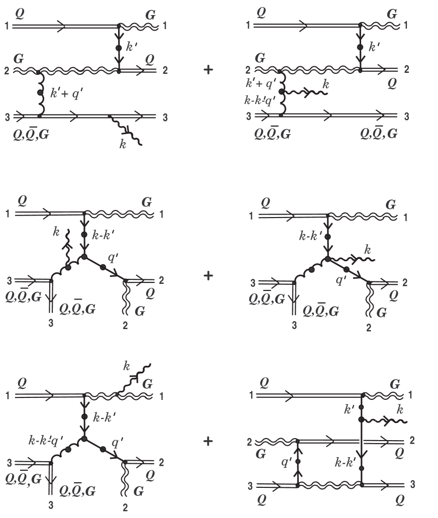
Figure 4: Some of bremsstrahlung processes of soft gluon at interaction of three hard partons.

Now we turn to question of the construction of an effective source $\tilde{\eta}_{\alpha}^{i}(q)$ generating soft quark bremsstrahlung at interaction of three hard particles. Here, similar to the previous case, two effective sources different in structure are possible: the first one defines the bremsstrahlung process, at which the statistics of one of three hard partons changes, while the second effective source does bremsstrahlung process, at which the statistics of all three hard particles change. Let us consider the first of them. The general structure of the effective source is given by the following formula:

$$\tilde{\eta}_{\alpha}^{i}(q)=\,K^{ab,\,ij}_{\alpha}({\bf v}_{1},{\bf v}_{2},{\bf v}_{3};\chi_{1},\chi_{2},\chi_{3};{\bf x}_{01},{\bf x}_{02},{\bf x}_{03}|\,q)\,Q_{01}^{a}Q_{02}^{b}\theta_{03}^{j}$$ (6.5)

$$+\,\,K^{ab,\,ij}_{\alpha}({\bf v}_{1},{\bf v}_{3},{\bf v}_{2};\ldots|\,q)\,Q_{01}^{a}Q_{03}^{b}\theta_{02}^{j}+\,K^{ab,\,ij}_{\alpha}({\bf v}_{3},{\bf v}_{2},{\bf v}_{1};\ldots|\,q)\,Q_{03}^{a}Q_{02}^{b}\theta_{01}^{j}.$$

It is clear that by virtue of symmetry with respect to permutation of the usual color charges $Q_{01}^{a}$ and $Q_{02}^{b}$ the first coefficient function $K_{\alpha}^{ab,\,ij}({\bf v}_{1},{\bf v}_{2},{\bf v}_{3};\dots|\,q)$ has to be symmetric with respect to the replacement: $a\rightleftharpoons b,\,1\rightleftharpoons 2$, i.e.

$$K^{ab,\,ij}_{\alpha}({\bf v}_{1},{\bf v}_{2},{\bf v}_{3};\,\ldots|\,q)=K^{ba,\,ij}_{\alpha}({\bf v}_{2},{\bf v}_{1},{\bf v}_{3};\,\ldots|\,q).$$ (6.6)

The calculations result in the following expression for the coefficient function:

$$\left.\frac{\delta^{3}\eta_{\alpha}^{i}(q)}{\delta Q^{a}_{01}\delta Q^{b}_{02}\delta\theta_{03}^{j}}\,\right|_{\,0}=K^{ab,\,ij}_{\alpha}({\bf v}_{1},{\bf v}_{2},{\bf v}_{3};\,\ldots|\,q)=$$ (6.7)

$$-\frac{\,g^{5}}{(2\pi)^{9}}\int\Biggl{\{}\left[\,\delta{\Gamma}^{(Q)ba,\,ij}_{\mu\nu}(q^{\prime},k^{\prime};q-q^{\prime}-k^{\prime},-q)\,^{\ast}\!S(q-q^{\prime}-k^{\prime})\chi_{3}\right]_{\alpha}\!\!\,^{\ast}{\cal D}^{\mu\mu^{\prime}}(q^{\prime})v_{2\mu^{\prime}}\,^{\ast}{\cal D}^{\nu\nu^{\prime}}(k^{\prime})v_{1\nu^{\prime}}$$

$$\hskip 28.45274pt-\,[t^{b},t^{a}]^{ij}\,K_{\alpha}^{(Q)\mu}({\bf v}_{3},\chi_{3}|\,q^{\prime}+k^{\prime},-q)\,^{\ast}{\cal D}_{\mu\nu}(q^{\prime}+k^{\prime})\,{\cal K}^{\nu}({\bf v}_{1},{\bf v}_{2}|\,q^{\prime}+k^{\prime},q^{\prime})$$

$$\hskip 42.67912pt+\,\Biggl{(}(t^{b}t^{a})^{ij}\Bigl{[}\,K_{\alpha}^{(Q)}(\chi_{2},\bar{\chi}_{2}|\,q,-q+q^{\prime})\,^{\ast}\!S(q-q^{\prime})\,{\cal K}({\bf v}_{1},{\bf v}_{3};\chi_{1},\chi_{3}|\,q-q^{\prime},-q+q^{\prime}+k^{\prime})\Bigr{]}_{\alpha}$$

$$+\,\alpha\,\chi_{2\alpha}\Bigg{\{}\frac{(t^{b}t^{a})^{ij}}{(v_{2}\cdot q)(v_{2}\cdot k^{\,\prime})}-\frac{(t^{a}t^{b})^{ij}}{(v_{2}\cdot(q-q^{\prime}-k^{\prime}))(v_{2}\cdot k^{\,\prime})}\Biggr{\}}$$

$$\times\Bigl{(}v_{2}^{\mu}\,{}^{\ast}{\cal D}_{\mu\nu}(k^{\prime})v_{1}^{\nu}\Bigr{)}\Bigl{[}\,\bar{\chi}_{2}\,^{\ast}\!S(q-q^{\prime}-k^{\prime})\chi_{3}\Bigr{]}+(a\rightleftharpoons b,\,1\rightleftharpoons 2)\Biggr{)}$$

$$-\,\{t^{b},t^{a}\}^{ij}\,\frac{\chi_{3\alpha}}{(v_{3}\cdot(q^{\prime}+k^{\prime}))(v_{3}\cdot k^{\prime})}\,\Bigl{(}v_{3}^{\mu}\,{}^{\ast}{\cal D}_{\mu\mu^{\prime}}(q^{\prime})v_{2}^{\mu^{\prime}}\Bigr{)}\Bigl{(}v_{3}^{\nu}\,{}^{\ast}{\cal D}_{\nu\nu^{\prime}}(k^{\prime})v_{1}^{\nu^{\prime}}\Bigr{)}\!\Biggl{\}}$$

$$\times\,{\rm e}^{-i{\bf k}^{\prime}\cdot\,{\bf x}_{01}}{\rm e}^{-i{\bf q}^{\prime}\cdot\,{\bf x}_{02}}{\rm e}^{-i({\bf q}-{\bf q}^{\prime}-{\bf k}^{\prime})\cdot\,{\bf x}_{03}}\,\delta(v_{1}\cdot k^{\prime})\delta(v_{2}\cdot q^{\prime})\delta(v_{3}\cdot(q-q^{\prime}-k^{\prime}))\,dk^{\prime}dq^{\prime}.$$

Here, the coefficient functions $K_{\alpha\beta}^{(Q)}(\chi_{2},\bar{\chi}_{2}|\,q,-q+q^{\prime})$ and $K_{\alpha}^{(Q)\mu}({\bf v}_{3},\chi_{3}|\,q^{\prime}+k^{\prime},-q)$ are defined by Eqs. (II.5.15) and (II.4.6), correspondingly. By straightforward calculation one can verify function (6.7) satisfies symmetry condition (6.6). Diagrammatic interpretation of some terms of effective source (6.7) is presented in Fig. 5. To be specific, as two hard partons that do not change their own statistics, we have chosen gluons.

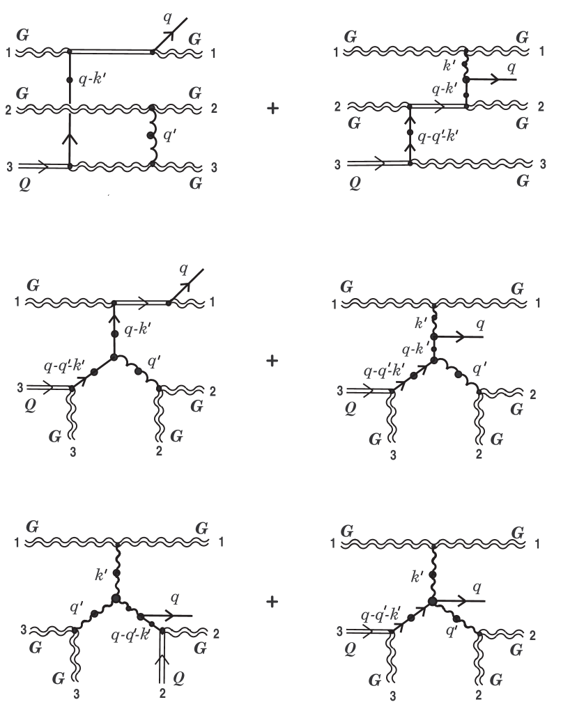
Figure 5: Some of bremsstrahlung processes of soft quark at collision of three hard partons, at which one of parton changes its statistics.

Furthermore, consider calculation of the second effective source defining the bremsstrahlung process in which the statistics of all three hard partons suffer a change. The general structure of the effective source is defined by the following expression:

$$\tilde{\eta}_{\alpha}^{i}(q)=\,K^{ij,kl}_{\alpha}({\bf v}_{1},{\bf v}_{2},{\bf v}_{3};\chi_{1},\chi_{2},\chi_{3};{\bf x}_{01},{\bf x}_{02},{\bf x}_{03}|\,q)\,\theta_{01}^{\dagger j}\theta_{02}^{k}\theta_{03}^{l}$$ (6.8)

$$+\,K^{ij,kl}_{\alpha}({\bf v}_{2},{\bf v}_{1},{\bf v}_{3};\,\dots|\,q)\,\theta_{02}^{\dagger j}\theta_{01}^{k}\theta_{03}^{l}+\,K^{ij,kl}_{\alpha}({\bf v}_{3},{\bf v}_{2},{\bf v}_{1};\,\dots|\,q)\,\theta_{03}^{\dagger j}\theta_{02}^{k}\theta_{01}^{l}.$$

By virtue of antisymmetry with respect to permutation of Grassmann charges $\theta_{02}^{k}$ and $\theta_{03}^{l}$, the first coefficient function $K_{\alpha}^{ij,kl}({\bf v}_{1},{\bf v}_{2},{\bf v}_{3};\,\ldots|\,q)$ has to be antisymmetric with respect to the replacement $k\rightleftharpoons l,\,2\rightleftharpoons 3$, i.e.

$$K^{ij,kl}_{\alpha}({\bf v}_{1},{\bf v}_{2},{\bf v}_{3};\,\ldots|\,q)=-\,K^{ij,lk}_{\alpha}({\bf v}_{1},{\bf v}_{3},{\bf v}_{2};\,\ldots|\,q).$$ (6.9)

The explicit form of the coefficient function is defined from the following third order derivative of the total source (the right-hand side of the Dirac equation (2.7)):

$$\left.\frac{\delta^{3}\eta_{\alpha}^{i}(q)}{\delta\theta_{01}^{\dagger j}\delta\theta_{02}^{k}\delta\theta_{03}^{l}}\,\right|_{\,0}=-\,K^{ij,kl}_{\alpha}({\bf v}_{1},{\bf v}_{2},{\bf v}_{3};\,\ldots|\,q)$$

$$\hskip 71.13188pt=\!\int\Biggl{\{}-\Biggl{[}\frac{\delta^{2}\eta_{\alpha}^{(1,1)i}(A,\psi)(q)}{\delta A^{a_{1}^{\prime}\mu_{1}^{\prime}}(k_{1}^{\,\prime})\delta\psi^{i_{1}^{\prime}}_{\alpha_{1}^{\prime}}(q_{1}^{\,\prime})}\,\Biggl{(}\frac{\delta\psi^{i_{1}^{\prime}}_{\alpha_{1}^{\prime}}(q_{1}^{\,\prime})}{\delta\theta_{02}^{k}}\Biggr{)}\,\frac{\delta^{2}\!A^{a_{1}^{\prime}\mu_{1}^{\prime}}(k_{1}^{\,\prime})}{\delta\theta_{01}^{\dagger j}\,\delta\theta_{03}^{l}}\,\,dk_{1}^{\,\prime}dq_{1}^{\,\prime}\hskip 85.35826pt$$

$$+\,\frac{\delta^{2}\eta_{\theta_{2}\alpha}^{(1)i}(q)}{\delta\theta_{02}^{k}\,\delta A^{a_{1}^{\prime}\mu_{1}^{\prime}}(k_{1}^{\,\prime})}\,\frac{\delta^{2}\!A^{a_{1}^{\prime}\mu_{1}^{\prime}}(k_{1}^{\,\prime})}{\delta\theta_{01}^{\dagger j}\,\delta\theta_{03}^{l}}\;dk_{1}^{\,\prime}\hskip 83.93553pt$$

$$\hskip 28.45274pt+\,\frac{\delta^{3}\Bigl{(}\eta_{\Xi\alpha}^{(2)i}(q)+\eta^{(2)i}_{\Omega\alpha}(q)\Bigr{)}}{\delta\bar{\psi}^{i_{1}^{\prime}}_{\alpha_{1}^{\prime}}(-q_{1}^{\,\prime})\delta\psi^{i_{2}^{\prime}}_{\alpha_{2}^{\prime}}(q_{2}^{\,\prime})\delta\theta_{02}^{k}}\,\Biggl{(}\frac{\bar{\psi}^{i_{1}^{\prime}}_{\alpha_{1}^{\prime}}(-q_{1}^{\,\prime})}{\delta\theta_{01}^{\dagger j}}\Biggr{)}\Biggl{(}\frac{\psi^{i_{2}^{\prime}}_{\alpha_{2}^{\prime}}(q_{2}^{\,\prime})}{\delta\theta_{03}^{l}}\Biggr{)}dq_{1}^{\,\prime}dq_{2}^{\,\prime}$$

$$\hskip 216.2411pt\,-\,(2\rightleftharpoons 3,\;k\rightleftharpoons l)\Biggr{]}$$

$$\hskip 36.98866pt+\,\frac{\delta^{3}\eta_{\tilde{\Omega}\alpha}^{i}(q)}{\delta\theta_{01}^{\dagger j}\,\delta\psi^{i_{2}^{\prime}}_{\alpha_{2}^{\prime}}(q_{2}^{\,\prime})\delta{\psi}^{i_{1}^{\prime}}_{\alpha_{1}^{\prime}}(q_{1}^{\,\prime})}\,\Biggl{(}\frac{\psi^{i_{2}^{\prime}}_{\alpha_{2}^{\prime}}(q_{2}^{\,\prime})}{\delta\theta_{02}^{k}}\Biggr{)}\Biggl{(}\frac{\psi^{i_{1}^{\prime}}_{\alpha_{1}^{\prime}}(q_{1}^{\,\prime})}{\delta\theta^{l}_{03}}\Biggr{)}\;dq_{1}^{\,\prime}dq_{2}^{\,\prime}\Biggl{\}}\Bigg{|}_{\,0\,.}$$

Here, as usually, we have kept contributions different from zero only. From the structure of the right-hand side of the last expression we see condition (6.9) to be automatically satisfied. Taking into account the explicit forms for sources $\eta_{\theta\alpha}^{(1)i},\,\eta_{\alpha}^{(1,1)}(A,\psi),\ldots$ it is easy to obtain

$$K^{ij,kl}_{\alpha}({\bf v}_{1},{\bf v}_{2},{\bf v}_{3};\,\ldots|\,q)$$ (6.10)

$$=\frac{g^{5}}{(2\pi)^{9}}\,\Biggl{\{}(t^{a})^{ik}(t^{a})^{jl}\!\!\int\!K^{(Q)}_{\alpha\mu}({\bf v}_{2},\chi_{2}|\,k^{\prime},-q)\,^{\ast}{\cal D}^{\mu\nu}(k^{\prime})[\,\bar{\chi}_{1\,}{\cal K}_{\nu}({\bf v}_{1},{\bf v}_{3}|\,k^{\prime},-q^{\prime})\chi_{3}]$$

$$\times\,{\rm e}^{-i({\bf k}^{\prime}-{\bf q}^{\prime})\cdot\,{\bf x}_{01}}{\rm e}^{-i({\bf q}-{\bf k}^{\prime})\cdot\,{\bf x}_{02}}{\rm e}^{-i{\bf q}^{\prime}\cdot\,{\bf x}_{03}}\,\delta(v_{1}\cdot(k^{\prime}-q^{\prime}))\delta(v_{2}\cdot(q-k^{\prime}))\delta(v_{3}\cdot q^{\prime})\,dk^{\prime}dq^{\prime}$$

$$\hskip 28.45274pt+\,\Bigl{\{}\beta\,(t^{a})^{ik}(t^{a})^{jl}+\,\beta_{1}(t^{a})^{il}(t^{a})^{jk}\Bigr{\}}\!\int\!\frac{\chi_{2\alpha}}{(v_{2}\cdot q^{\prime})(v_{2}\cdot k^{\prime})}\,\left[\,\bar{\chi}_{1}\,^{\ast}\!S(k^{\prime})\chi_{2}\right]\left[\,\bar{\chi}_{2}\,^{\ast}\!S(q^{\prime})\chi_{3}\right]\hskip 28.45274pt$$

$$\times\,{\rm e}^{-i{\bf k}^{\prime}\cdot\,{\bf x}_{01}}{\rm e}^{-i({\bf q}-{\bf q}^{\prime}-{\bf k}^{\prime})\cdot\,{\bf x}_{02}}{\rm e}^{-i{\bf q}^{\prime}\cdot\,{\bf x}_{03}}\,\delta(v_{1}\cdot k^{\prime})\delta(v_{2}\cdot(q-q^{\prime}-k^{\prime}))\delta(v_{3}\cdot q^{\prime})\,dk^{\prime}dq^{\prime}\hskip 14.22636pt$$

$$\hskip 56.9055pt-\,\Bigl{(}2\rightleftharpoons 3,\,k\rightleftharpoons l\Bigr{)}\Biggr{\}}$$

$$\hskip 42.67912pt-\,\tilde{\beta}_{1}\,\Bigl{\{}(t^{a})^{il}(t^{a})^{jk}-\,(t^{a})^{ik}(t^{a})^{jl}\Bigr{\}}\,\frac{g^{5}}{(2\pi)^{9}}\!\int\!\frac{\chi_{1\alpha}}{(v_{1}\cdot q^{\prime})(v_{1}\cdot k^{\prime})}\,\left[\,\bar{\chi}_{1}\,^{\ast}\!S(k^{\prime})\chi_{3}\right]\left[\,\bar{\chi}_{1}\,^{\ast}\!S(q^{\prime})\chi_{2}\right]\hskip 28.45274pt$$

$$\times\,{\rm e}^{-i({\bf q}-{\bf q}^{\prime}-{\bf k}^{\prime})\cdot\,{\bf x}_{01}}{\rm e}^{-i{\bf q}^{\prime}\cdot\,{\bf x}_{02}}{\rm e}^{-i{\bf k}^{\prime}\cdot\,{\bf x}_{03}}\,\delta(v_{1}\cdot(q-q^{\prime}-k^{\prime}))\delta(v_{2}\cdot q^{\prime})\delta(v_{3}\cdot k^{\prime})\,dk^{\prime}dq^{\prime}.\hskip 14.22636pt$$

In Fig. 6 we present diagrammatic interpretation of some of the terms on the right-hand side of effective source (6.10). Here, as initial hard particles 1 and 2 we have chosen quarks, and as an initial hard particle 3 we have chosen a gluon, which as a result of the interaction transform into hard gluons and hard quark, respectively.

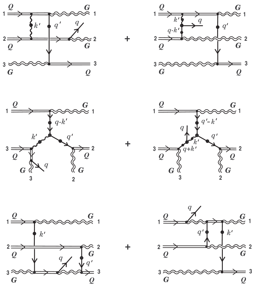
Figure 6: Some of bremsstrahlung processes of soft quark for three hard partons collision when all of the hard particles change their statistics.

7 ‘Off-diagonal’ contributions to radiation energy loss. Connection with double Born scattering

The section 3, 4 and 5 were concerned with analysis of radiation intensity for bremsstrahlung of soft gluon and soft quark generated by the lowest order processes of scattering which in turn induced by effective current (2.5) and effective source (2.11). These effective quantities define what is called ‘diagonal’ contribution $\left\langle\tilde{j}^{\ast(1)a}_{\mu}(k;{\bf b})\!\,^{\ast}{\cal D}^{\mu\nu}_{C}(k)\tilde{j}^{(1)a}_{\nu}(k;{\bf b})\right\rangle$ to the soft-gluon radiation field energy $W({\bf b})$ (Eq. (3.1)) and ‘diagonal’ contribution $\left\langle\bar{\tilde{\eta}}^{(1)i}(-q;{\bf b})\bigr{\{}\,^{\ast}\!S(-q)+\!\,^{\ast}\!S(q)\bigl{\}}\,\tilde{\eta}^{(1)i}(q;{\bf b})\right\rangle$ to the soft-quark radiation field energy $W({\bf b})$ (Eq. (3.8)). In the present and next sections we would like to consider a question on a role of the simplest ’off-diagonal’ terms

$$\left\langle\tilde{j}^{\ast(0)a}_{\mu}(k;{\bf b})\!\,^{\ast}{\cal D}^{\mu\nu}_{C}(k)\tilde{j}^{(2)a}_{\nu}(k;{\bf b})\right\rangle\,+\,\left\langle\tilde{j}^{\ast(2)a}_{\mu}(k;{\bf b})\!\,^{\ast}{\cal D}^{\mu\nu}_{C}(k)\tilde{j}^{(0)a}_{\nu}(k;{\bf b})\right\rangle$$ (7.1)

and

$$\left\langle\bar{\tilde{\eta}}^{(0)i}(-q;{\bf b})\bigr{\{}\,^{\ast}\!S(-q)+\!\,^{\ast}\!S(q)\bigl{\}}\,\tilde{\eta}^{(2)i}(q;{\bf b})\right\rangle\,+\,\left\langle\bar{\tilde{\eta}}^{(2)i}(-q;{\bf b})\bigr{\{}\,^{\ast}\!S(-q)+\!\,^{\ast}\!S(q)\bigl{\}}\,\tilde{\eta}^{(0)i}(q;{\bf b})\right\rangle$$ (7.2)

in the overall balance of the radiation field energy of the system. In the above expressions

$$\tilde{j}^{(0)a}_{\mu}(k;{\bf b})=\frac{g}{(2\pi)^{3}}\;Q_{01}^{a}v_{1\mu}\,\delta(v_{1}\cdot k)+\frac{g}{(2\pi)^{3}}\;Q_{02}^{a}v_{2\mu}\,\delta(v_{2}\cdot k){\rm e}^{i{\bf k}\cdot{\bf b}}$$ (7.3)

is the initial “bare” color current,

$$\tilde{\eta}^{(0)\,i}_{\alpha}(q;{\bf b})=\frac{\,g}{(2\pi)^{3}}\;\theta_{01}^{i}\chi_{1\alpha}\,\delta(v_{1}\cdot q)+\frac{\,g}{(2\pi)^{3}}\;\theta_{02}^{i}\chi_{2\alpha}\,\delta(v_{2}\cdot q){\rm e}^{i{\bf q}\cdot{\bf b}}$$ (7.4)

is the initial “bare” color source, and $\tilde{j}_{\mu}^{(2)a}(k;{\bf b}),\,\tilde{\eta}_{\alpha}^{(2)i}(q;{\bf b})$ are effective current and source of next in order of the coupling constant in comparison with $\tilde{j}_{\mu}^{(1)a}(k;{\bf b})$ and $\tilde{\eta}_{\alpha}^{(1)i}(q;{\bf b})$.

To begin with, we consider the ‘off-diagonal’ contribution associated with usual color current, i.e. we do Eq. (7.1). The only non-trivial ‘off-diagonal’ contribution to the radiation field energy arises here from the expansion terms of effective current, which are functions of the third-order in usual color charges $Q_{01},\,Q_{02}$, and Grassmann color charges $\theta_{01}$ and $\theta_{02}$. In the paper [13] we have considered in detail a contribution associated with the second-order effective current $\tilde{j}_{\mu}^{(2)a}$ having the following structure:

$$\tilde{j}^{(2)a}_{\mu}(k)=\frac{1}{2!}\,\Bigl{\{}K^{aa_{1}a_{2}a_{3}}_{\mu}({\bf v}_{1},{\bf v}_{2};{\bf x}_{01},{\bf x}_{02}|\,k)\,Q_{01}^{a_{1}}Q_{02}^{a_{2}}Q_{02}^{a_{3}}\hskip 28.45274pt$$ (7.5)

$$\hskip 42.67912pt+\,K^{aa_{1}a_{2}a_{3}}_{\mu}({\bf v}_{2},{\bf v}_{1};{\bf x}_{02},{\bf x}_{01}|\,k)\,Q_{01}^{a_{1}}Q_{01}^{a_{2}}Q_{02}^{a_{3}}\Bigr{\}}$$

The given effective current can be obtained from (6.1) by means of a simple identification of two of three hard partons. Here there exist three different ways of such identification

$$(I)\;\left\{\begin{array}[]{rl}1\rightarrow 1\\ 2\rightarrow 1\\ 3\rightarrow 2\\ \end{array}\right.,\qquad(II)\;\left\{\begin{array}[]{rl}1\rightarrow 1\\ 2\rightarrow 2\\ 3\rightarrow 1\\ \end{array}\right.,\qquad(III)\;\left\{\begin{array}[]{rl}1\rightarrow 2\\ 2\rightarrow 1\\ 3\rightarrow 1\\ \end{array}\right.$$

plus symmetrization of the final expression about the permutation $1\rightleftharpoons 2$. We combine together all the expressions obtained in this way for the effective current and divide the final expression by the factor $3\cdot 2=6$. By virtue of such identification the coefficient functions on the right-hand side of Eq. (7.5) are associated with coefficient function of initial current (6.1) by simple way

$$K^{aa_{1}a_{2}a_{3}}_{\mu}({\bf v}_{1},{\bf v}_{2};\,\dots|\,k)\equiv K^{aa_{1}a_{2}a_{3}}_{\mu}({\bf v}_{1},{\bf v}_{2},{\bf v}_{2};\,\ldots|\,k),$$

$$K^{aa_{1}a_{2}a_{3}}_{\mu}({\bf v}_{2},{\bf v}_{1};\,\dots|\,k)\equiv K^{aa_{1}a_{2}a_{3}}_{\mu}({\bf v}_{1},{\bf v}_{1},{\bf v}_{2};\,\ldots|\,k).$$

Now we take into account the existence of fermion degree of freedom for hard and soft excitations. In this case additional effective current (6.2) appears. By analogy with the above-mentioned scheme we define effective current similar to (7.5) by an identification of two of three hard particles. We write the expression obtained in the form of the sum of two different in structure (and physical meaning) effective currents:

$$\tilde{j}^{(2)a}_{\mu}(k)=\tilde{j}^{(2)a}_{I\mu}(k)+\tilde{j}^{(2)a}_{II\mu}(k),$$

where

$$\tilde{j}^{(2)a}_{I\mu}(k)=K^{ab,\,ij}_{\mu}({\bf v}_{1},{\bf v}_{1},{\bf v}_{2};\,\dots|\,k)\,\theta_{01}^{\dagger i}\theta_{01}^{j}Q_{02}^{b}+K^{ab,\,ij}_{\mu}({\bf v}_{2},{\bf v}_{2},{\bf v}_{1};\,\dots|\,k)\,\theta_{02}^{\dagger i}\theta_{02}^{j}Q_{01}^{b}\hskip 11.38092pt$$ (7.6)

and

$$\tilde{j}^{(2)a}_{II\mu}(k)=\Bigl{[}\,K^{ab,\,ij}_{\mu}({\bf v}_{1},{\bf v}_{2},{\bf v}_{2};\,\dots|\,k)\,\theta_{01}^{\dagger i}\theta_{02}^{j}Q_{02}^{b}+K^{ab,\,ij}_{\mu}({\bf v}_{2},{\bf v}_{1},{\bf v}_{2};\,\dots|\,k)\,\theta_{02}^{\dagger i}\theta_{01}^{j}Q_{02}^{b}\Bigr{]}$$ (7.7)

$$\hskip 22.76228pt+\,\Bigl{[}\,K^{ab,\,ij}_{\mu}({\bf v}_{2},{\bf v}_{1},{\bf v}_{1};\,\dots|\,k)\,\theta_{02}^{\dagger i}\theta_{01}^{j}Q_{01}^{b}+K^{ab,\,ij}_{\mu}({\bf v}_{1},{\bf v}_{2},{\bf v}_{1};\,\dots|\,k)\,\theta_{01}^{\dagger i}\theta_{02}^{j}Q_{01}^{b}\Bigr{]}.$$

It should be particularly emphasized that an explicit form of all the coefficient functions in the definition of effective currents (7.6) and (7.7), is defined from single expression (6.4). Besides, the current reality condition (6.3) automatically guarantees reality of each of effective currents (7.6) and (7.7).

At first, we consider contribution to the ‘off-diagonal’ energy losses associated with color effective current (7.6). Let us present the coefficient function $K_{\mu}^{ab,\,ij}({\bf v}_{2},{\bf v}_{1};\,\ldots|\,k)\equiv K_{\mu}^{ab,\,ij}({\bf v}_{2},{\bf v}_{2},{\bf v}_{1};\,\ldots|\,k)$ in the form of expansion in terms of the symmetric and anti-symmetric combinations of the $t^{a}$ generators

$$K_{\mu}^{ab,\,ij}({\bf v}_{2},{\bf v}_{1};\,\ldots|\,k)=\frac{1}{2}\,\{t^{a},t^{b}\}^{ij}K_{\mu}^{({\cal S})}({\bf v}_{2},{\bf v}_{1};\,\ldots|\,k)+\frac{1}{2}\,[\,t^{a},t^{b}\,]^{ij}K_{\mu}^{({\cal A})}({\bf v}_{2},{\bf v}_{1};\,\ldots|\,k).$$

An explicit form of the symmetric $K_{\mu}^{({\cal S})}$ and anti-symmetric $K_{\mu}^{({\cal A})}$ parts is easily defined from (6.4) and in particular for the former we get

$$K_{\mu}^{({\cal S})}({\bf v}_{2},{\bf v}_{1};\,\ldots|\,k)$$ (7.8)

$$=\frac{\,g^{5}}{(2\pi)^{9}}\int\biggl{\{}\left[\,\bar{\chi}_{2}\,^{\ast}\!S(k^{\prime})\,\delta{\Gamma}^{(G;\,{\cal S})}_{\mu\nu}(k,-k+k^{\prime}+q^{\prime};-k^{\prime},-q^{\prime})\,^{\ast}\!S(q^{\prime})\chi_{2}\right]\!\,^{\ast}{\cal D}^{\nu\nu^{\prime}}\!(k-k^{\prime}-q^{\prime})v_{1\nu^{\prime}}$$

$$\hskip 2.84544pt-\left[\,\bar{K}_{\mu}^{(G)}({\bf v}_{2},\bar{\chi}_{2}|\,k,-k+k^{\prime})\,^{\ast}\!S(k-k^{\prime})\,{\cal K}({\bf v}_{1},{\bf v}_{2};\chi_{1},\chi_{2}|\,k-k^{\prime},-q^{\prime})\right]$$

$$\hskip 5.69046pt+\left[\,\bar{\cal K}({\bf v}_{1},{\bf v}_{2};\chi_{1},\chi_{2}|\,-k+q^{\prime},k^{\prime})\,^{\ast}\!S(k-q^{\prime})\,K_{\mu}^{(G)}({\bf v}_{2},\chi_{2}|\,k,-k+q^{\prime})\right]$$

$$+\,2\sigma\,\frac{v_{1\mu}}{(v_{1}\cdot k^{\prime})(v_{1}\cdot q^{\prime})}\,\left[\,\bar{\chi}_{2}\,^{\ast}\!S(k^{\prime})\chi_{1}\right]\left[\,\bar{\chi}_{1}\,^{\ast}\!S(q^{\prime})\chi_{2}\right]\hskip 28.45274pt$$

$$\times\,{\rm e}^{-i({\bf k}-{\bf k}^{\prime}-{\bf q}^{\prime})\cdot\,{\bf x}_{01}}{\rm e}^{-i({\bf k}^{\prime}+{\bf q}^{\prime})\cdot\,{\bf x}_{02}}\,\delta(v_{1}\cdot(k-k^{\prime}-q^{\prime}))\delta(v_{2}\cdot k^{\prime})\delta(v_{2}\cdot q^{\prime})\,dk^{\prime}dq^{\prime}.$$

In the subsequent discussion we need not the antisymmetric part $K_{\mu}^{({\cal A})}$. Therefore we do not give an explicit form of it. In Fig. 7 diagrammatic interpretation of some of the terms in function (7.8) is depicted. By virtue of the structure of effective current (7.6) it is clear that statistics of hard partons 1 and 2 does not change in the interaction process.

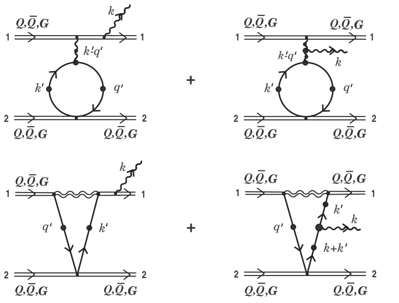
Figure 7: Some of soft one-loop corrections to bremsstrahlung process depicted in Fig. 1 in the paper [13].

Let us substitute effective current (7.6) and initial current (7.3) into (7.1) and then into (3.1). Performing the average over usual color charges we lead to the expression for the ‘off-diagonal’ contribution to energy of soft-gluon radiation field (we keep only transverse mode for simplicity)

$$(W({\bf b}))^{t}_{\rm off-diag}=-\,4\pi g\,C_{F}\Biggl{(}\frac{C_{2}^{(1)}C^{(2)}_{\theta}}{d_{A}}\Biggr{)}\!\!\sum_{\xi=1,\,2\,}\int\!d{\bf k}d\omega\,\omega\,{\rm Im}(^{\ast}{\!\Delta}^{t}(k))$$ (7.9)

$$\times\,{\rm Re}\Bigl{[}({\bf e}^{\ast}(\hat{\bf k},\xi)\cdot{\bf v}_{1})\Bigl{(}K^{({\cal S})i}({\bf v}_{2},{\bf v}_{1};\chi_{2},\chi_{1};{\bf x}_{02},{\bf x}_{01}|\,k){\rm e}^{i}(\hat{\bf k},\xi)\Bigr{)}\Bigr{]}\,\delta(v_{1}\cdot k)$$

$$\hskip 42.67912pt-\,4\pi g\,C_{F}\Biggl{(}\frac{C_{2}^{(2)}C^{(1)}_{\theta}}{d_{A}}\Biggr{)}\!\!\sum_{\xi=1,\,2\,}\int\!d{\bf k}d\omega\,\omega\,{\rm Im}(^{\ast}{\!\Delta}^{t}(k))$$

$$\hskip 34.14322pt\times\,{\rm Re}\Bigl{[}({\bf e}^{\ast}(\hat{\bf k},\xi)\cdot{\bf v}_{2})\Bigl{(}K^{({\cal S})i}({\bf v}_{1},{\bf v}_{2};\chi_{1},\chi_{2};{\bf x}_{01},{\bf x}_{02}|\,k){\rm e}^{i}(\hat{\bf k},\xi)\Bigr{)}\,{\rm e}^{-i{\bf k}\cdot{\bf b}}\Bigr{]}\,\delta(v_{2}\cdot k).$$

In the limit of static color center ${\bf v}_{2}=0$ the second term on the right-hand side of the above equation vanishes. This corresponds to neglect of bremsstrahlung from a thermal parton 2.

Further, we substitute expression (7.9) with ‘symmetric’ coefficient function (7.8) into formula for radiation intensity (3.5) previously setting up in (7.8) ${\bf x}_{01}=0$ and ${\bf x}_{02}=({\bf b},0)$. The delta-functions in the integrands of (7.9) and (7.8) in the static limit result in the following measure of integration

$$\delta(v_{1}\cdot k)\,[\,\delta(q_{0}^{\prime})\delta(k_{0}^{\prime})dq_{0}^{\prime}dk_{0}^{\prime}\,]\,\delta({\bf v}_{1}\cdot({\bf q}^{\prime}+{\bf k}^{\prime}))d{\bf q}^{\prime}d{\bf k}^{\prime}\,d{\bf k}d\omega.$$ (7.10)

Next, integration over the ${\bf b}$ impact parameter leads to another delta-function in the integrand

$$\int\!\!d{\bf b}\,{\rm e}^{-i({\bf q}^{\prime}+{\bf k}^{\prime})\cdot{\bf b}}=(2\pi)^{2}\delta^{(2)}(({\bf q}^{\prime}+{\bf k}^{\prime})_{\perp}).$$

The given expression together with (7.10) enables us to perform easily the integration with respect to $d{\bf k}^{\prime}$ that gives ${\bf k}^{\prime}\!=\!-\,{\bf q}^{\prime}$. Omitting for simplicity the prime of variable ${\bf q}^{\prime}$, after some algebraic transformations and regrouping of terms, we result in the final expression for the ‘off-diagonal’ contribution to radiation energy losses of the fast color particle 1 within the static approximation

$$\left(\!-\frac{dE_{1}}{dx}\right)_{\!{\rm off-diag}}^{\!t}=\Lambda_{1}+\Lambda_{2}.$$

Here, on the right-hand side the function $\Lambda_{1}$ is

$$\Lambda_{1}=-2\biggl{(}\frac{{\alpha}_{s}}{\pi}\biggr{)}^{\!3}\Biggl{(}\frac{C_{F}\,C_{2}^{(1)}}{d_{A}}\Biggr{)}\!\!\sum\limits_{\,\zeta=Q,\,\bar{Q}}\!\!C_{\theta}^{(\zeta)}\!\!\int\!{\bf p}_{2}^{2}\left[f_{|{\bf p}_{2}|}^{(\zeta)}+f_{|{\bf p}_{2}|}^{(G)}\right]\frac{d|\,{\bf p}_{2}|}{2\pi^{2}}$$ (7.11)

$$\times\!\sum_{\xi=1,\,2\,}\!\int\!d{\bf k}d\omega\,\omega\;{\rm Im}(^{\ast}{\!\Delta}^{t}(k))\,\delta(v_{1}\cdot k)\!\int\!d{\bf q}\,\Biggl{(}2\!\,{\rm Re}\,\sigma\,\frac{|({\bf e}(\hat{\bf k},\xi)\cdot{\bf v}_{1})|^{\,2}}{({\bf v}_{1}\cdot{\bf q})^{2}}\left|\left[\bar{\chi}_{1}\!\,^{\ast}\!S(q)\chi_{2}\right]\right|^{\,2}$$

$$-\frac{\alpha}{({\bf v}_{1}\cdot{\bf q})}\,{\rm Re}\,\Bigl{\{}\!({\bf e}^{\ast}(\hat{\bf k},\xi)\cdot{\bf v}_{1})\left[\bar{\chi}_{1}\!\,^{\ast}\!S(q)\chi_{2}\right]\![\,\bar{\chi}_{2}\!\,^{\ast}\!S(-q)\!\,^{\ast}\Gamma^{(G)i}(k;q,-k-q){\rm e}^{i}(\hat{\bf k},\xi)\!\,^{\ast}\!S(k+q)\chi_{\!1}]\Bigr{\}}\hskip 8.5359pt$$

$$+\frac{\alpha}{({\bf v}_{1}\cdot{\bf q})}\,{\rm Re}\,\Bigl{\{}\!({\bf e}^{\ast}(\hat{\bf k},\xi)\cdot{\bf v}_{1})\left[\bar{\chi}_{2}\!\,^{\ast}\!S(-q)\chi_{1}\right]\![\,\bar{\chi}_{1}\!\,^{\ast}\!S(k-q)\!\,^{\ast}\Gamma^{(G)i}(k;-k+q,-q){\rm e}^{i}(\hat{\bf k},\xi)\!\,^{\ast}\!S(q)\chi_{\!2}]\Bigr{\}}\!\!\Biggr{)}_{\!\!\!q_{0}=0}$$

and the $\Lambda_{2}$ function has the form

$$\Lambda_{2}=-2\biggl{(}\frac{{\alpha}_{s}}{\pi}\biggr{)}^{\!3}\Biggl{(}\frac{C_{F}\,C_{2}^{(1)}}{d_{A}}\Biggr{)}\!\!\sum\limits_{\,\zeta=Q,\,\bar{Q}}\!\!C_{\theta}^{(\zeta)}\!\!\int\!{\bf p}_{2}^{2}\left[f_{|{\bf p}_{2}|}^{(\zeta)}+f_{|{\bf p}_{2}|}^{(G)}\right]\frac{d|\,{\bf p}_{2}|}{2\pi^{2}}$$ (7.12)

$$\times\!\!\sum_{\xi,\,\xi^{\prime}=1,\,2\,}\!\int\!d{\bf k}d\omega\,\omega\;{\rm Im}(^{\ast}{\!\Delta}^{t}(k))\!\int\!d{\bf q}\,{\rm Re}\,\Bigl{\{}({\bf e}^{\ast}(\hat{\bf k},\xi)\cdot{\bf v}_{1})\,({\bf e}(\hat{\bf k},\xi^{\prime})\cdot{\bf v}_{1})\,^{\ast}\!\Delta^{t}(k)$$

$$\times\!\left[\,\bar{\chi}_{2}\!\,^{\ast}\!S(-q){\cal M}^{(G;\,{\cal S})ii^{\prime}}(k,-k;\,q,-q)\!\,^{\ast}\!S(q)\chi_{2}\right]{\rm e}^{i}(\hat{\bf k},\xi)\,{\rm e}^{\ast i^{\prime}}(\hat{\bf k},\xi^{\prime})\Bigr{\}}_{\!q_{0}\,=\,0}\,\delta(v_{1}\cdot k),$$

where the quark propagator $\!\,{}^{\ast}S(q)$ in the static limit $q_{0}=0$ is defined by the expression $h_{+}(\hat{\bf q})\,^{\ast}\!\Delta_{+}(0,{\bf q})+h_{-}(\hat{\bf q})\,^{\ast}\!\Delta_{-}(0,{\bf q})$ with $\!\,{}^{\ast}\!\Delta_{\pm}(0,{\bf q})\!=\!\pm\,|\,{\bf q}|/({\bf q}^{2}+\omega_{0}^{2}(1\mp i\pi/2))$. Further, in the preceding equation the function ${\cal M}^{(G;\,{\cal S})ii^{\prime}}(k,-k;q,-q)$ is the ‘symmetric’ part of the scattering amplitude of a soft gluon excitation off a soft quark excitation. This scattering amplitude was introduced in Paper I (the equation following Eq. (I.7.15)). The expressions obtained (7.11) and (7.12) should be added to ones (6.7) and (6.8) of the paper [13]. The diagrammatic interpretation of different terms in $\Lambda_{1}$ and $\Lambda_{2}$ is presented in Fig. 8. To be specific, as a hard parton 1 we have chosen here a quark.

Figure 8: The diagrammatic interpretation of terms defining ‘off-diagonal’ contribution to soft-gluon radiation energy losses. The dotted lines denote thermal partons absorbing virtual bremsstrahlung gluons and ${\bf q}$ is three-dimensional vector.

The functions $\Lambda_{1}$ and $\Lambda_{2}$ are nonvanishing only for plasma excitations lying off mass-shell. From the form of graphs in Fig. 8 it is evident that they represent so-called the contact double Born graphs [14, 15].

Let us analyze a role of the first $\Lambda_{1}$ function in the theory under consideration. For this purpose it is necessary to confront the $\Lambda_{1}$ with main ‘diagonal’ contribution (3.6) (more precisely, with the terms containing the transverse scalar propagator $\,{}^{\ast}\!\Delta^{t}(k)$). Setting ${\bf v}_{2}=0$, we rewrite this ‘diagonal’ contribution once more, considered the module squared $|\,{\rm e}^{i}{\cal K}^{i}|^{\,2}$

$$\left(\!-\frac{dE_{1}}{dx}\right)_{\!{\rm diag}}^{\!t}=-\biggl{(}\frac{{\alpha}_{s}}{\pi}\biggr{)}^{\!3}\Biggl{(}\sum\limits_{\;\zeta=Q,\,\bar{Q}}\!\!C_{\theta\theta}^{(1;\,\zeta)}\!\!\int\!{\bf p}_{2}^{2}\left[f_{|{\bf p}_{2}|}^{(\zeta)}+f_{|{\bf p}_{2}|}^{(G)}\right]\frac{d|{\bf p}_{2}|}{2\pi^{2}}\,\Biggr{)}$$ (7.13)

$$\times\!\sum_{\xi=1,\,2\,}\!\int\!d{\bf k}d\omega\,\omega\;{\rm Im}(^{\ast}{\!\Delta}^{t}(k))\!\int\!d{\bf q}\,\Biggl{(}\Biggl{\{}\frac{|\,({\bf e}(\hat{\bf k},\xi)\cdot{\bf v}_{1})|^{\,2}}{({\bf v}_{1}\cdot{\bf q})^{2}}\left|\,\left[\bar{\chi}_{1}\!\,^{\ast}\!S(q)\chi_{2}\right]\right|^{\,2}$$

$$+\,\frac{2}{({\bf v}_{1}\cdot{\bf q})}\,{\rm Re}\,\Bigl{\{}({\bf e}^{\ast}(\hat{\bf k},\xi)\cdot{\bf v}_{1})\left[\bar{\chi}_{2}\!\,^{\ast}\!S(-q)\chi_{1}\right]\![\,\bar{\chi}_{1}\!\,^{\ast}\!S(k-q)\!\,^{\ast}\Gamma^{(G)i}(k;-k+q,-q){\rm e}^{i}(\hat{\bf k},\xi)\!\,^{\ast}\!S(q)\chi_{\!2}]\Bigr{\}}$$

$$+\,\Bigl{|}\Bigl{[}\,\bar{\chi}_{1}\!\,^{\ast}\!S(k-q)\!\,^{\ast}\Gamma^{(G)i}(k;-k+q,-q){\rm e}^{i}(\hat{\bf k},\xi)\!\,^{\ast}\!S(q)\chi_{\!2}\Bigr{]}\Bigr{|}^{\,2}\Biggr{\}}\,\delta(v_{1}\cdot k+{\bf v}_{1}\cdot{\bf q})$$

$$\hskip 85.35826pt+\,\Biggl{\{}\frac{|\,({\bf e}(\hat{\bf k},\xi)\cdot{\bf v}_{1})|^{\,2}}{({\bf v}_{1}\cdot{\bf q})^{2}}\left|\,\left[\bar{\chi}_{1}\!\,^{\ast}\!S(q)\chi_{2}\right]\right|^{\,2}$$

$$+\,\frac{2}{({\bf v}_{1}\cdot{\bf q})}\,{\rm Re}\,\Bigl{\{}({\bf e}(\hat{\bf k},\xi)\cdot{\bf v}_{1})\left[\bar{\chi}_{2}\!\,^{\ast}\!S(-q)\chi_{1}\right]\![\,\bar{\chi}_{1}\!\,^{\ast}\!S(-k-q)\!\,^{\ast}\Gamma^{(G)i}(-k;k+q,-q){\rm e}^{\ast i}(\hat{\bf k},\xi)\!\,^{\ast}\!S(q)\chi_{\!2}]\Bigr{\}}$$

$$+\,\Bigl{|}\Bigl{[}\,\bar{\chi}_{1}\!\,^{\ast}\!S(-k-q)\!\,^{\ast}\Gamma^{(G)i}(-k;k+q,-q){\rm e}^{\ast i}(\hat{\bf k},\xi)\,^{\ast}\!S(q)\chi_{\!2}\Bigr{]}\Bigr{|}^{\,2}\Biggr{\}}\,\delta(v_{1}\cdot k-{\bf v}_{1}\cdot{\bf q})\Biggr{)}.$$

For the off mass-shell collective excitations the integrand here contains singularities of the form $1/({\bf v}_{1}\cdot{\bf q})^{2}$ and $1/({\bf v}_{1}\cdot{\bf q})$ when frequency and momentum of plasma excitations approach to the “Cherenkov cone”

$$(v_{1}\cdot k)\rightarrow 0.$$

Related singularities are contained in the $\Lambda_{1}$ function. Let us require that these singularities in exact cancel each other in the sum of two expressions (7.11) and (7.13). This requirement give rises to the following two conditions of cancellation of the singularities

$$C_{\theta\theta}^{(1;\,\zeta)}=\alpha\Biggl{(}\frac{C_{F}\,C_{2}^{(1)}}{d_{A}}\Biggr{)}C_{\theta}^{(\zeta)},$$ (7.14)

$${\rm Re}\,\sigma=\frac{1}{2}\,\alpha.$$

We see the latter condition in Eq. (7.14) exactly to coincide with similar condition of cancellation of the singularities obtained in Paper II (the equation following Eq. (II.12.9)). The former condition in Eq. (7.14) can be vied as definition of unknown constants $C_{\theta\theta}^{(1;\,Q)}$ and $C_{\theta\theta}^{(1;\,\bar{Q})}$ introduced in section 3.

Now we proceed to the next point concerning a physical meaning of the $\Lambda_{2}$ contribution. Let us show that the contribution can be partly interpreted as one taking into account a change of dispersion properties of the medium caused by the processes of nonlinear interaction of soft excitations in the QGP. With this in mind we write out the expression for the polarization energy losses of an energetic parton 1 taking into consideration the first correction with respect to soft stochastic fields in the system

$$\left(\!-\frac{dE_{1}}{dx}\right)^{\!t}=-\biggl{(}\frac{\alpha_{s}}{2{\pi}^{2}}\biggr{)}\,C_{2}^{(1)}\!\!\int\!d{\bf k}d\omega\,\omega\,{\rm Im}(\,^{\ast}{\!\Delta}^{t}(k))\biggl{\{}\sum\limits_{\,\xi,\,\xi^{\prime}=1,\,2}\Bigl{[}\,({\bf e}^{\ast}(\hat{\bf k},\xi)\cdot{\bf v}_{1})({\bf e}(\hat{\bf k},\xi^{\prime})\cdot{\bf v}_{1})\,\delta^{\xi\xi^{\prime}}\hskip 28.45274pt$$ (7.15)

$$\hskip 113.81102pt+\,{\rm Re}\Bigl{[}\,({\bf e}^{\ast}(\hat{\bf k},\xi)\cdot{\bf v}_{1})({\bf e}(\hat{\bf k},\xi^{\prime})\cdot{\bf v}_{1})\Pi_{tt}^{(1)}(k;\xi,\xi^{\prime})\,^{\ast}{\!\Delta}^{t}(k)\Bigr{]}\Bigr{]}\biggr{\}}\,\delta(v_{1}\cdot k).$$

Here we have omitted contributions with the longitudinal mode. In the above expression, the function

$$\Pi_{tt}^{(1)}(k;\xi,\xi^{\prime})\equiv-2g^{2}T_{F}\!\int\!d{\bf q}dq^{0}\,{\rm Sp}\,\Bigl{\{}{\cal M}^{(G;\,{\cal S})ii^{\prime}}(-k,k;-q,q)\Upsilon(q)\Bigr{\}}{\rm e}^{\ast\,i}(\hat{\bf k},\xi){\rm e}^{i^{\prime}}(\hat{\bf k},\xi^{\prime})$$ (7.16)

is correction to the transverse part of the soft-gluon self-energy $\delta\Pi_{\mu\nu}(k)$, linear in the soft-quark spectral density $\Upsilon(q)$. The Dirac trace is presented by ‘Sp’. As a spectral density $\Upsilon(q)$ it is necessary to take spectral one of soft quark excitations caused by (static) thermal partons.

Let us make use the initial definition of the spectral density in question a correlator of two soft $\psi$ fields

$$\left\langle\bar{\psi}_{\alpha}^{i}(-q)\psi_{\beta}^{j}(q_{1})\right\rangle=\delta^{ji\,}\Upsilon_{\beta\alpha}(q_{1})\,\delta(q-q_{1}).$$

Hence it formally follows that

$$\Upsilon_{\beta\alpha}(q)=\frac{1}{N_{c}}\int\!dq_{1}\left\langle\bar{\psi}_{\alpha}^{i}(-q)\psi_{\beta}^{j}(q_{1})\right\rangle.$$ (7.17)

In the situation under consideration the soft quark field $\psi$ induced by a hard test particle 2 that is located at the position ${\bf x}_{02}$, is

$$\psi_{\beta}^{i}(q_{1};{\bf x}_{02})=-\frac{\,g}{(2\pi)^{3}}\,\left(\,{}^{\ast}\!S(q_{1})\chi_{2}\right)_{\beta}\delta(v_{2}\cdot q_{1})\,\theta_{02}^{i}\,{\rm e}^{-i{\bf q}_{\!1}\cdot\,{\bf x}_{02}}$$ (7.18)

$$\bar{\psi}_{\alpha}^{i}(-q;{\bf x}_{02})=\frac{\,g}{(2\pi)^{3}}\;\theta_{02}^{\dagger i}\,\left(\bar{\chi}_{2}\,^{\ast}\!S(-q)\right)_{\alpha}\delta(v_{2}\cdot q){\rm e}^{i{\bf q}\cdot\,{\bf x}_{02}}.\hskip 11.38092pt$$

As a definition of the spectral density we take the following expression, instead of (7.17)

$$\Upsilon_{\beta\alpha}(q)=\frac{1}{N_{c}}\sum\limits_{\;\zeta=Q,\,\bar{Q}\,}\!\int\!{\bf p}_{2}^{2}\left[\,f_{|{\bf p}_{2}|}^{(\zeta)}+f_{|{\bf p}_{2}|}^{(G)}\,\right]\frac{d|\,{\bf p}_{2}|}{2\pi^{2}}\int\!\frac{d\Omega_{{\bf v}_{2}}}{4\pi}\!\int\!d{\bf x}_{02}\!\int\!dq_{1}\left\langle\bar{\psi}_{\alpha}^{i}(-q;{\bf x}_{02})\psi_{\beta}^{j}(q_{1};{\bf x}_{02})\right\rangle.$$

Substituting functions (7.18) into the preceding equation and performing simple calculations in static limit ${\bf v}_{2}=0$, we finally obtain (here one suppresses spinor indices)

$$\left.\Upsilon(q)\right|_{\;{\rm static}}=-\frac{\,g^{2}}{(2\pi)^{3}}\,\frac{1}{N_{c}}\sum\limits_{\;\zeta=Q,\,\bar{Q}\,}\!\!\!C_{\theta}^{(\zeta)}\!\int\!{\bf p}_{2}^{2}\left[\,f_{|{\bf p}_{2}|}^{(\zeta)}+f_{|{\bf p}_{2}|}^{(G)}\,\right]\frac{d|\,{\bf p}_{2}|}{2\pi^{2}}$$ (7.19)

$$\times\,\Bigl{(}\!\,^{\ast}\!S(q_{1})\chi_{2}\Bigr{)}\!\otimes\!\Bigl{(}\bar{\chi}_{2}\,^{\ast}\!S(-q)\Bigr{)}\delta(q^{0}).$$

If one substitutes the expression obtained into (7.16), then it is not difficult to see that the correction term in Eq.  (7.15) in exact reproduces the $\Lambda_{2}$ function (7.12) if the identity $C_{F}/d_{A}=T_{F}/N_{c}$ is accounted for.

On the other hand, the correction term in (7.15) was shown in Paper II to be due to partly the change of dispersion properties of the medium in interacting soft excitations with each other. Let us consider the expression for the polarization energy losses of a fast parton 1 in the HTL-approximation

$$\left(\!-\frac{dE^{(0)}_{1}}{dx}\right)_{\!{\cal B}}=-\biggl{(}\frac{\alpha_{s}}{2{\pi}^{2}}\biggr{)}\,C_{2}^{(1)}\!\!\int\!d{\bf k}d\omega\,\omega\,{\rm Im}\,\left(v_{1\mu}\!\,^{\ast}{\cal D}_{C}^{\mu\nu}(k)v_{1\nu}\right)\delta(v_{1}\cdot k).$$

We replace the gluon propagator $\,{}^{\ast}{\cal D}_{C}^{\mu\nu}(k)$ by the $\,{}^{\ast}\tilde{\cal D}_{C}^{\mu\nu}(k)$ effective one taking into account the processes of nonlinear interaction of soft fermi- and bose-excitations. In the linear approximation in the spectral densities we have

$$\,{}^{\ast}{\cal D}_{C}^{\mu\nu}(k)\Rightarrow\,^{\ast}\tilde{\cal D}_{C}^{\mu\nu}(k)=\!\,^{\ast}{\cal D}_{C}^{\mu\nu}(k)+\!\,^{\ast}{\cal D}_{C}^{\mu\mu^{\prime}}(k)\Pi^{(1)}_{\mu^{\prime}\nu^{\prime}}[\Upsilon,I](k)\!\,^{\ast}{\cal D}_{C}^{\nu^{\prime}\nu}(k)+\,\ldots$$

$$=\!\sum\limits_{\,\xi,\,\xi^{\prime}=1,\,2}\biggl{\{}\!\,^{\ast}{\!\Delta}^{t}(k)\,({\rm e}^{\ast\,i}(\hat{\bf k},\xi){\rm e}^{j}(\hat{\bf k},\xi^{\prime}))\,\delta^{\xi\xi^{\prime}}\hskip 142.26378pt$$

$$\hskip 85.35826pt+\,^{\ast}{\!\Delta}^{t}(k)({\rm e}^{\ast i}(\hat{\bf k},\xi){\rm e}^{j}(\hat{\bf k},\xi^{\prime}))\!\left(\,{\rm e}^{l}(\hat{\bf k},\xi)\Pi^{(1)ll^{\prime}}[\Upsilon,I](k){\rm e}^{\ast l^{\prime}}(\hat{\bf k},\xi^{\prime})\right)\!\,^{\ast}{\!\Delta}^{t}(k)$$

$$\hskip 32.72049pt+\,(\mbox{the terms with}\,\,\!\,^{\ast}{\!\Delta}^{l}(k)\,\mbox{and high-order corrections})\biggr{\}}.$$

Contracting the above expression with $v_{1}^{i}v_{1}^{j}$ and taking an imaginary part, we derive

$${\rm Im}\left(\!v^{i}_{1}\!\,{}^{\ast}\tilde{\cal D}_{C}^{ij}(k)v^{j}_{1}\right)={\rm Im}(\,^{\ast}{\!\Delta}^{t}(k))\!\!\sum\limits_{\,\xi,\,\xi^{\prime}=1,\,2}\biggl{\{}\,({\bf e}^{\ast}(\hat{\bf k},\xi)\cdot{\bf v}_{1})({\bf e}(\hat{\bf k},\xi^{\prime})\cdot{\bf v}_{1})\,\delta^{\xi\xi^{\prime}}$$

$$+\,{\rm Re}\Bigl{[}\,^{\ast}{\!\Delta}^{t}(k)({\bf e}^{\ast}(\hat{\bf k},\xi)\cdot{\bf v}_{1})({\bf e}(\hat{\bf k},\xi^{\prime})\cdot{\bf v}_{1})\left({\rm e}^{l}(\hat{\bf k},\xi)\Pi^{(1)ll^{\prime}}[\Upsilon,I](k){\rm e}^{\ast l^{\prime}}(\hat{\bf k},\xi^{\prime})\right)\Bigr{]}\biggl{\}}$$

$$+\,{\rm Re}(\,^{\ast}{\!\Delta}^{t}(k))\!\!\!\sum\limits_{\,\xi,\,\xi^{\prime}=1,\,2}{\rm Im}\Bigl{[}\,^{\ast}{\!\Delta}^{t}(k)({\bf e}^{\ast}(\hat{\bf k},\xi)\cdot{\bf v}_{1})({\bf e}(\hat{\bf k},\xi^{\prime})\cdot{\bf v}_{1})\left({\rm e}^{l}(\hat{\bf k},\xi)\Pi^{(1)ll^{\prime}}[\Upsilon,I](k){\rm e}^{\ast l^{\prime}}(\hat{\bf k},\xi^{\prime})\right)\Bigr{]}$$

$$+\,(\mbox{the terms with}\,\,\!\,^{\ast}{\!\Delta}^{l}(k)\,\mbox{and high-order corrections}).$$

The first term on the right-hand side with an imaginary part ${\rm Im}(\,^{\ast}{\!\Delta}^{t}(k))$ in exact reproduces the integrand in (7.15). The physical meaning of the second term with ${\rm Re}(\,^{\ast}{\!\Delta}^{t}(k))$ is not clear.

In the rest of this section we briefly discuss the effective current defined by equation (7.7). By using general formula (6.4) it is not difficult to obtain an explicit form of each of coefficient functions $K_{\mu}^{ab,\,ij}$ entering into definition of this current. The given current contains ‘non-compensated’ Grassmann color charges $\theta_{01}^{i}$ and $\theta_{02}^{i}$. Because of this it defines the scattering process of two hard partons (followed by emission of a soft gluon) under which statistics of both hard particles change. Examples of some of the diagrams illustrating this scattering process are given in Fig. 9. As initial hard partons 1 and 2 here we have taken quark and gluon, respectively.

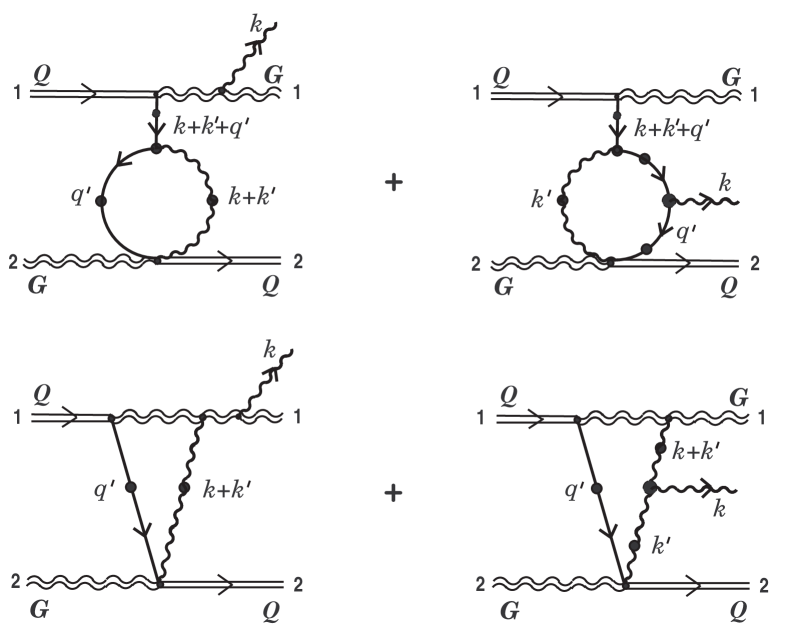
Figure 9: Some of soft one-loop corrections to bremsstrahlung process depicted in Fig.1 of the present work.

However, if we attempt to define a contribution of the given effective current to the ‘off-diagonal’ energy losses, making use of Eqs.  (7.1), (7.3), and (3.1), then we are faced here with color factors of the type

$$\biggl{(}\frac{C_{2}^{(1)}}{d_{A}}\biggr{)}\frac{1}{2}\,\{t^{a},t^{a}\}^{ij}\,\theta_{01}^{\dagger i}\theta_{02}^{j}\equiv\biggl{(}\frac{C_{2}^{(1)}C_{F}}{d_{A}}\biggr{)}(\theta_{01}^{\dagger i}\theta_{02}^{i})$$

and so on. The contractions with Grassmann charges relating to different particles ‘non-interpreted’ from the physical point of view arise. For this reason similar contributions will be systematically dropped.

8 Off-diagonal contribution to radiation energy loss (continuation)

The present and next sections are concerned with consideration of the contribution to ‘off-diagonal’ energy losses caused by an effective source of the second order $\tilde{\eta}_{\alpha}^{(2)i}(q;{\bf b})$. Consider, first of all, as the effective source $\tilde{\eta}_{\alpha}^{(2)i}(q;{\bf b})$ an expression following from (6.5) for appropriate identification of two of three hard particles. As in the case of the second order effective source $\tilde{j}_{\mu}^{(2)a}(k;{\bf b})$ (the previous section) we present the final expression for $\tilde{\eta}_{\alpha}^{(2)i}(q;{\bf b})$ as the sum of two different in structure (and physical meaning) effective sources:

$$\tilde{\eta}_{\alpha}^{(2)i}(q;{\bf b})=\tilde{\eta}_{I\alpha}^{(2)i}(q;{\bf b})+\tilde{\eta}_{II\alpha}^{(2)i}(q;{\bf b}).$$

Here,

$$\tilde{\eta}_{I\alpha}^{(2)i}(q;{\bf b})=\frac{1}{2!}\,\Bigl{\{}K^{(I)\,ab,ij}_{\alpha}({\bf v}_{1},{\bf v}_{2};\,\dots|\,q)\,Q_{01}^{a}Q_{01}^{b}\theta_{02}^{j}+K^{(I)\,ab,ij}_{\alpha}({\bf v}_{2},{\bf v}_{1};\,\dots|\,q)\,Q_{02}^{a}Q_{02}^{b}\theta_{01}^{j}\Bigr{\}},$$ (8.1)

where

$$K^{(I)\,ab,ij}_{\alpha}({\bf v}_{1},{\bf v}_{2};\,\dots|\,q)\equiv K^{ab,\,ij}_{\alpha}({\bf v}_{1},{\bf v}_{1},{\bf v}_{2};\,\dots|\,q),$$ (8.2)

$$K^{(I)\,ab,ij}_{\alpha}({\bf v}_{2},{\bf v}_{1};\,\dots|\,q)\equiv K^{ab,\,ij}_{\alpha}({\bf v}_{2},{\bf v}_{2},{\bf v}_{1};\,\dots|\,q)$$

and

$$\tilde{\eta}_{II\alpha}^{(2)i}(q;{\bf b})=K^{(II)\,ab,ij}_{\alpha}({\bf v}_{1},{\bf v}_{2};\,\dots|\,q)\,Q_{01}^{a}Q_{02}^{b}\theta_{02}^{j}+K^{(II)\,ab,ij}_{\alpha}({\bf v}_{2},{\bf v}_{1};\,\dots|\,q)\,Q_{02}^{a}Q_{01}^{b}\theta_{01}^{j}\Bigr{\}},$$ (8.3)

where in turn

$$K^{(II)\,ab,ij}_{\alpha}({\bf v}_{1},{\bf v}_{2};\,\dots|\,q)\equiv K^{ab,ij}_{\alpha}({\bf v}_{1},{\bf v}_{2},{\bf v}_{2};\,\dots|\,q),$$

$$K^{(II)\,ab,ij}_{\alpha}({\bf v}_{2},{\bf v}_{1};\,\dots|\,q)\equiv K^{ab,\,ij}_{\alpha}({\bf v}_{2},{\bf v}_{1},{\bf v}_{1};\,\dots|\,q).$$

An explicit form of the coefficient functions in the definition of effective sources (8.1) and (8.3) is defined from general formula (6.7) by obvious fashion.

Let us consider the ‘off-diagonal’ contribution to the radiation energy losses from source (8.1). By virtue of the symmetry with respect to permutation of the usual color charges $Q_{01}^{a}$ and $Q_{01}^{b}$ (or $Q_{02}^{a}$ and $Q_{02}^{b}$) a color structure of the coefficient functions in (8.1) is uniquely determined by

$$K^{(I)\,ab,ij}_{\alpha}({\bf v}_{1},{\bf v}_{2};\,\dots|\,q)=\frac{g^{5}}{(2\pi)^{9}}\,\{t^{a},t^{b}\}^{ij}K^{(I)}_{\alpha}({\bf v}_{1},{\bf v}_{2};\,\dots|\,q)$$ (8.4)

and so on. Here we have separated out in an explicit form the coupling constant dependence of these functions. Let us substitute effective source (8.1), (8.4) and initial source (7.4) into (7.2) and then into (3.8). Performing the average over usual color charges and taking into account the color factor $\theta_{01}^{\dagger i}\{t^{a},t^{a}\}^{ij}\theta_{01}^{j}\equiv 2\,C_{F}\,C_{\theta}^{(1)}$ (and similarly for a particle 2) we lead to expression for the ‘off-diagonal’ contribution to soft-quark radiation field energy

$$(W({\bf b}))_{\rm off-diag}=\frac{1}{(2\pi)^{2}}\,\biggl{(}\frac{{\alpha}_{s}}{\pi}\biggr{)}^{\!3}\!\sum\limits_{\lambda\,=\,\pm}\int\!d{\bf q}dq^{0}\,q^{0}\Biggl{[}\,{\rm Im}\,(\!\,^{\ast}\!\Delta_{+}(q))$$ (8.5)

$$\times\Biggl{\{}C^{(1)}_{\theta}\Biggl{(}\frac{C_{F}\,C_{2}^{(2)}}{d_{A}}\Biggr{)}[\bar{\chi}_{1}u(\hat{\bf q},\lambda)][\,\bar{u}(\hat{\bf q},\lambda)K^{(I)}({\bf v}_{2},{\bf v}_{1};\ldots;{\bf b}|\,q)]\,\delta(v_{1}\cdot q)$$

$$\hskip 36.98866pt+\;C^{(2)}_{\theta}\Biggl{(}\frac{C_{F}\,C_{2}^{(1)}}{d_{A}}\Biggr{)}[\bar{\chi}_{2}u(\hat{\bf q},\lambda)][\,\bar{u}(\hat{\bf q},\lambda)K^{(I)}({\bf v}_{1},{\bf v}_{2};\ldots;{\bf b}|\,q)]\,\delta(v_{2}\cdot q){\rm e}^{-i{\bf q}\cdot{\bf b}}$$

$$\hskip 42.67912pt+\,\mbox{(compl. conj.)}\Biggr{\}}\;+\;\Bigl{(}\,^{\ast}{\!\Delta}_{+}(q)\rightarrow\,^{\ast}{\!\Delta}_{-}(q),\;u(\hat{\bf q},\lambda)\rightarrow v(\hat{\bf q},\lambda)\Bigr{)}\Biggr{]}.$$

In the case of the static color center model, i.e. under the condition when we can neglect by bremsstrahlung of a soft quark from thermal partons, we can drop the contributions proportional to $[\bar{\chi}_{2}u(\hat{\bf q},\lambda)],\,[\bar{\chi}_{2}v(\hat{\bf q},\lambda)]$ and so on. Further, we can proceed in the usual way as in section 7. At first we write out an explicit form of the function $K^{(I)}({\bf v}_{2},{\bf v}_{1};\,\dots|\,q)$ according to formulae (8.2) and (6.7). Then in the expression obtained we set ${\bf x}_{01}=0$ and ${\bf x}_{02}=({\bf b},0)$. Finally, substitute $K^{(I)}({\bf v}_{2},{\bf v}_{1};\,\dots|\,q)$ into (8.5) and then $(W({\bf b}))_{\rm off-diag}$ into formula of radiation intensity (3.4). Performing the integration over the impact parameter ${\bf b}$ and considering that in the static limit

$$\left.\!\,{}^{\ast}{\cal D}^{\mu 0}_{C}(q^{\prime})\right|_{\,q_{0}^{\prime}=0}=\frac{1}{{\bf q}^{\prime\,2}+\mu_{D}^{2}}\;g^{\mu 0},$$

we obtain the desired expression for the ‘off-diagonal’ energy losses induced by bremsstrahlung of a soft quark

$$\left(\!-\frac{dE_{1}}{dx}\right)_{\!{\rm off-diag}}=\hat{\Lambda}_{1}+\hat{\Lambda}_{2},$$

where

$$\hat{\Lambda}_{1}=-\biggl{(}\frac{{\alpha}_{s}}{\pi}\biggr{)}^{\!3}\Biggl{(}\frac{C_{F}\,C_{\theta}^{(1)}}{d_{A}}\Biggr{)}\!\!\sum\limits_{\,\zeta=Q,\,\bar{Q},\,G}\!\!C_{2}^{(\zeta)}\!\!\int\!{\bf p}_{2}^{2}\,f_{|{\bf p}_{2}|}^{(\zeta)}\,\frac{d|\,{\bf p}_{2}|}{2\pi^{2}}$$ (8.6)

$$\times\!\sum\limits_{\lambda\,=\,\pm}\int\!d{\bf q}dq^{0}\,q^{0}\,{\rm Im}\,(\!\,^{\ast}\!\Delta_{+}(q))\,\delta(v_{1}\cdot q)\int\!d{\bf q}^{\prime}\,\frac{1}{({\bf q}^{\prime\,2}+\mu_{D}^{2})^{2}}\;\Biggl{[}\,\frac{|(\bar{\chi}_{1}u(\hat{\bf q},\lambda))|^{\,2}}{({\bf v}_{1}\cdot{\bf q}^{\prime})^{2}}$$

$$+\,2\,\frac{1}{({\bf v}_{1}\cdot{\bf q}^{\prime})}\,{\rm Re}\,\Bigl{\{}(\bar{\chi}_{1}u(\hat{\bf q},\lambda))\!\left(\bar{u}(\hat{\bf q},\lambda)\!\,^{\ast}\Gamma^{(Q)0}(q^{\prime};q-q^{\prime},-q)\!\,^{\ast}\!S(q-q^{\prime})\chi_{\!1}\right)\!\Bigr{\}}\!\Biggr{]}_{q_{0}^{\prime}\,=\,0}$$

$$+\;\Bigl{(}\,^{\ast}{\!\Delta}_{+}(q)\rightarrow\,^{\ast}{\!\Delta}_{-}(q),\;u(\hat{\bf q},\lambda)\rightarrow v(\hat{\bf q},\lambda)\Bigr{)},$$

and

$$\hat{\Lambda}_{2}=-\biggl{(}\frac{{\alpha}_{s}}{\pi}\biggr{)}^{\!3}\Biggl{(}\frac{C_{F}\,C_{\theta}^{(1)}}{d_{A}}\Biggr{)}\!\!\sum\limits_{\,\zeta=Q,\,\bar{Q},\,G}\!\!C_{2}^{(\zeta)}\!\!\int\!{\bf p}_{2}^{2}\,f_{|{\bf p}_{2}|}^{(\zeta)}\,\frac{d|\,{\bf p}_{2}|}{2\pi^{2}}$$ (8.7)

$$\times\!\sum\limits_{\lambda\,=\,\pm}\int\!d{\bf q}dq^{0}\,q^{0}\,{\rm Im}\,(\!\,^{\ast}\!\Delta_{+}(q))\,\delta(v_{1}\cdot q)$$

$$\hskip 28.45274pt\times\!\int\!d{\bf q}^{\prime}\,\frac{1}{({\bf q}^{\prime\,2}+\mu_{D}^{2})^{2}}\left.{\rm Re}\,\Bigl{\{}(\bar{\chi}_{1}u(\hat{\bf q},\lambda))\!\left(\bar{u}(\hat{\bf q},\lambda){\cal F}_{00}^{(Q;\,S)}(-q^{\prime},q^{\prime};-q,q)\!\,^{\ast}\!S(q)\chi_{\!1}\right)\!\Bigr{\}}\right|_{\,q_{0}^{\prime}\,=\,0}$$

$$+\;\Bigl{(}\,^{\ast}{\!\Delta}_{+}(q)\rightarrow\,^{\ast}{\!\Delta}_{-}(q),\;u(\hat{\bf q},\lambda)\rightarrow v(\hat{\bf q},\lambda)\Bigr{)}.$$

In the latter expression we have used the definition of the function ${\cal F}_{\mu_{1}\mu_{2}}^{(Q;\,S)}(-k_{1},k_{2};q_{1},q)$ from Paper I (Eq. (I.5.23)). This function appears in the scattering amplitude of soft fermi- and bose-excitations off each other. The diagrammatic interpretation of different terms on the right-hand sides of Eqs. (8.6) and (8.7) is drawn in Fig. 10. As an initial high-energy parton here we have chosen a quark.

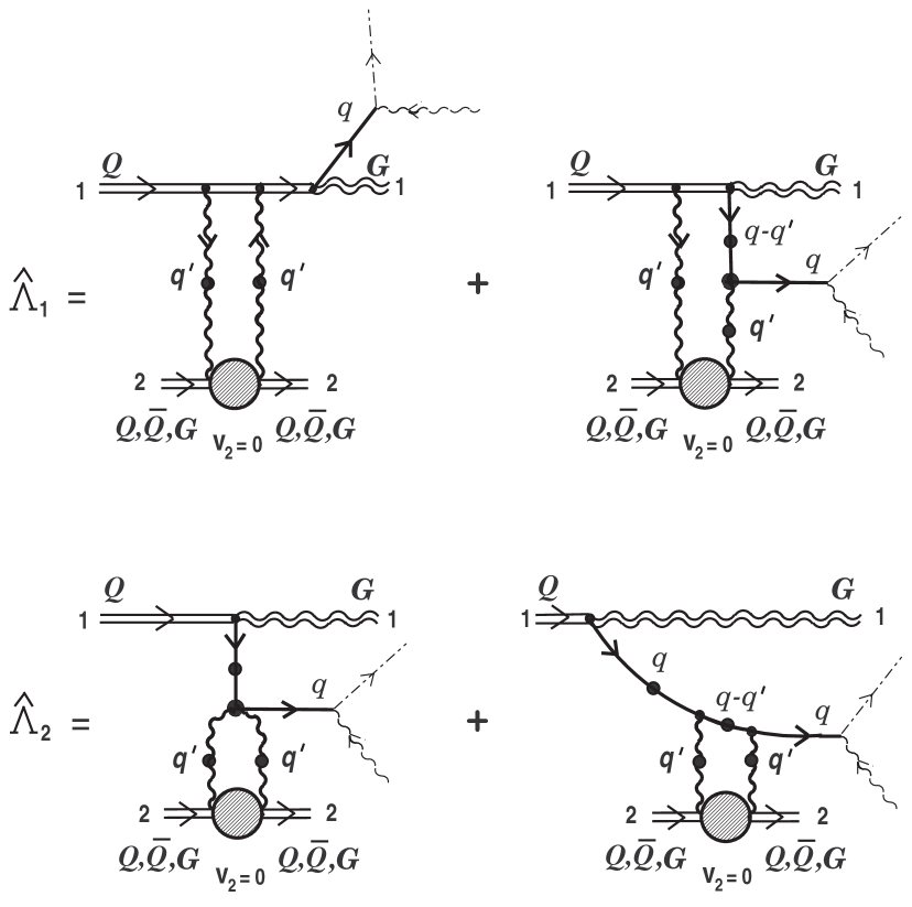
Figure 10: The diagrammatic interpretation of the first part of terms defining the ‘off-diagonal’ contribution to soft-quark radiation energy losses. The second part will be defined bellow.

As for effective source (8.3) it gives no contribution to the ‘off-diagonal’ energy losses. This is related with the fact that usual color charges $Q_{01}^{a}$ and $Q_{02}^{a}$ enter into this source in the mixed way. Multiplying (8.3) by the initial sources $\tilde{\bar{\eta}}_{\alpha}^{(0)i}(-q;{\bf b})$ or $\eta_{\alpha}^{(0)i}(q;{\bf b})$ and integrating over $dQ_{01},\,dQ_{02}$, we see that this contribution vanishes in exact in view of an equality

$$\int\!dQ_{01}\,Q_{01}^{a}=\int\!dQ_{02}\,Q_{02}^{a}=0.$$

Let us move on to consideration another effective source of the second order $\tilde{\eta}_{\alpha}^{(2)i}(q;{\bf b})$ that follows from (6.8) in identifying two of three hard particles. We also present the effective source obtained in the form of the sum of two different in structure effective ones:

$$\tilde{\eta}_{\alpha}^{(2)i}(q;{\bf b})=\tilde{\eta}_{I\alpha}^{(2)i}(q;{\bf b})+\tilde{\eta}_{II\alpha}^{(2)i}(q;{\bf b}).$$

Here now,

$$\tilde{\eta}_{I\alpha}^{(2)i}(q;{\bf b})=K^{(I)\,ij,kl}_{\alpha}({\bf v}_{1},{\bf v}_{2};\,\dots|\,q)\,\theta_{01}^{\dagger j}\theta_{01}^{k}\theta_{02}^{l}+K^{(I)\,ij,kl}_{\alpha}({\bf v}_{2},{\bf v}_{1};\,\dots|\,q)\,\theta_{02}^{\dagger j}\theta_{02}^{k}\theta_{01}^{l},$$ (8.8)

where

$$K^{(I)\,ij,kl}_{\alpha}({\bf v}_{1},{\bf v}_{2};\,\dots|\,q)\equiv K^{ij,kl}_{\alpha}({\bf v}_{1},{\bf v}_{1},{\bf v}_{2};\,\dots|\,q),$$ (8.9)

$$K^{(I)\,ij,kl}_{\alpha}({\bf v}_{2},{\bf v}_{1};\,\dots|\,q)\equiv K^{ij,kl}_{\alpha}({\bf v}_{2},{\bf v}_{2},{\bf v}_{1};\,\dots|\,q),$$

and

$$\tilde{\eta}_{II\alpha}^{(2)i}(q;{\bf b})=\frac{1}{2!}\,\Bigl{\{}K^{(II)\,ij,kl}_{\alpha}({\bf v}_{1},{\bf v}_{2};\,\dots|\,q)\,\theta_{01}^{\dagger j}\theta_{02}^{k}\theta_{02}^{l}+K^{(II)\,ij,kl}_{\alpha}({\bf v}_{2},{\bf v}_{1};\,\dots|\,q)\,\theta_{02}^{\dagger j}\theta_{01}^{k}\theta_{01}^{l}\Bigr{\}},$$ (8.10)

where in its turn

$$K^{(II)\,ij,kl}_{\alpha}({\bf v}_{1},{\bf v}_{2};\,\dots|\,q)\equiv K^{ij,kl}_{\alpha}({\bf v}_{1},{\bf v}_{2},{\bf v}_{2};\,\dots|\,q),$$

$$K^{(II)\,ij,kl}_{\alpha}({\bf v}_{2},{\bf v}_{1};\,\dots|\,q)\equiv K^{ij,kl}_{\alpha}({\bf v}_{2},{\bf v}_{1},{\bf v}_{1};\,\dots|\,q).$$

Explicit expressions of all the coefficient functions in the definition of effective sources (8.8) and (8.10) are easy to define from general formula (6.10).

Consider, at first, the contribution of source (8.8) to the ‘off-diagonal’ energy losses. Of equation (6.10) it is easily viewed that the coefficient function $K_{\alpha}^{(I)\,ij,kl}({\bf v}_{2},{\bf v}_{1};\,\ldots|\,q)$ has the following color structure:

$$K_{\alpha}^{(I)\,ij,kl}({\bf v}_{2},{\bf v}_{1};\,\ldots|\,q)$$ (8.11)

$$=\frac{g^{5}}{(2\pi)^{9}}\,\Bigl{[}(t^{a})^{ik}(t^{a})^{jl}K_{1\alpha}^{(I)}({\bf v}_{2},{\bf v}_{1};\,\ldots|\,q)+(t^{a})^{i\,l}(t^{a})^{jk}K_{2\alpha}^{(I)}({\bf v}_{2},{\bf v}_{1};\,\ldots|\,q)\Bigr{]},$$

where

$$K_{1\alpha}^{(I)}({\bf v}_{2},{\bf v}_{1};\,\ldots|\,q)$$

$$=\int\!\Bigl{\{}K^{(Q)}_{\alpha\mu}({\bf v}_{2},\chi_{2}|\,q-q^{\prime},-q)\,^{\ast}{\cal D}^{\mu\nu}(q-q^{\prime})[\,\bar{\chi}_{2\,}{\cal K}_{\nu}({\bf v}_{2},{\bf v}_{1}|\,q-q^{\prime},-q+q^{\prime}+k^{\prime})\chi_{1}]$$

$$-\,\beta\,\frac{\chi_{2\alpha}}{(v_{2}\cdot(q-q^{\prime}-k^{\prime}))(v_{2}\cdot k^{\prime})}\,\left[\,\bar{\chi}_{2}\,^{\ast}\!S(k^{\prime})\chi_{2}\right]\left[\,\bar{\chi}_{2}\,^{\ast}\!S(q-q^{\prime}-k^{\prime})\chi_{1}\right]$$

$$+\,\beta_{1}\,\frac{\chi_{1\alpha}}{(v_{2}\cdot q^{\prime})(v_{2}\cdot k^{\prime})}\,\left[\,\bar{\chi}_{2}\,^{\ast}\!S(k^{\prime})\chi_{1}\right]\left[\,\bar{\chi}_{1}\,^{\ast}\!S(q^{\prime})\chi_{2}\right]\hskip 93.89418pt$$ (8.12)

$$\hskip 8.5359pt-\,\tilde{\beta}_{1}\,\frac{\chi_{2\alpha}}{(v_{2}\cdot(q-q^{\prime}-k^{\prime}))(v_{2}\cdot q^{\prime})}\,\left[\,\bar{\chi}_{2}\,^{\ast}\!S(q^{\prime})\chi_{2}\right]\left[\,\bar{\chi}_{2}\,^{\ast}\!S(q-q^{\prime}-k^{\prime})\chi_{1}\right]\Bigr{\}}$$

$$\times\,{\rm e}^{-i({\bf q}-{\bf q}^{\prime}-{\bf k}^{\prime})\cdot\,{\bf x}_{01}}{\rm e}^{-i({\bf q}^{\prime}+{\bf k}^{\prime})\cdot\,{\bf x}_{02}}\,\delta(v_{1}\cdot(q-q^{\prime}-k^{\prime}))\,\delta(v_{2}\cdot k^{\prime})\delta(v_{2}\cdot q^{\prime})\,dk^{\prime}dq^{\prime}$$

and

$$K_{2\alpha}^{(I)}({\bf v}_{2},{\bf v}_{1};\,\ldots|\,q)$$

$$=\int\!\Bigl{\{}-K^{(Q)}_{\alpha\mu}({\bf v}_{1},\chi_{1}|\,q^{\prime}+k^{\prime},-q)\,^{\ast}{\cal D}^{\mu\nu}(q^{\prime}+k^{\prime})[\,\bar{\chi}_{2\,}{\cal K}_{\nu}({\bf v}_{2},{\bf v}_{2}|\,q^{\prime}+k^{\prime},-q^{\prime})\chi_{2}]$$

$$\hskip 5.69046pt-\,\beta_{1}\,\frac{\chi_{2\alpha}}{(v_{2}\cdot(q-q^{\prime}-k^{\prime}))(v_{2}\cdot k^{\prime})}\,\left[\,\bar{\chi}_{2}\,^{\ast}\!S(k^{\prime})\chi_{2}\right]\left[\,\bar{\chi}_{2}\,^{\ast}\!S(q-q^{\prime}-k^{\prime})\chi_{1}\right]$$

$$+\,\beta\,\frac{\chi_{1\alpha}}{(v_{2}\cdot q^{\prime})(v_{2}\cdot k^{\prime})}\,\left[\,\bar{\chi}_{2}\,^{\ast}\!S(k^{\prime})\chi_{1}\right]\left[\,\bar{\chi}_{1}\,^{\ast}\!S(q^{\prime})\chi_{2}\right]\hskip 93.89418pt$$ (8.13)

$$\hskip 14.22636pt+\,\tilde{\beta}_{1}\,\frac{\chi_{2\alpha}}{(v_{2}\cdot(q-q^{\prime}-k^{\prime}))(v_{2}\cdot q^{\prime})}\,\left[\,\bar{\chi}_{2}\,^{\ast}\!S(q^{\prime})\chi_{2}\right]\left[\,\bar{\chi}_{2}\,^{\ast}\!S(q-q^{\prime}-k^{\prime})\chi_{1}\right]\Bigr{\}}$$

$$\times\,{\rm e}^{-i({\bf q}-{\bf q}^{\prime}-{\bf k}^{\prime})\cdot\,{\bf x}_{01}}{\rm e}^{-i({\bf q}^{\prime}+{\bf k}^{\prime})\cdot\,{\bf x}_{02}}\,\delta(v_{1}\cdot(q-q^{\prime}-k^{\prime}))\,\delta(v_{2}\cdot k^{\prime})\delta(v_{2}\cdot q^{\prime})\,dk^{\prime}dq^{\prime}.$$

Further, we determine the ‘off-diagonal’ energy of soft-quark radiation field induced by effective source (8.8). In the same way as before we obtain

$$(W({\bf b}))_{\rm off-diag}=-2\,\frac{1}{(2\pi)^{2}}\,\biggl{(}\frac{{\alpha}_{s}}{\pi}\biggr{)}^{\!3}C_{\theta\theta}^{(1;2)}\!\sum\limits_{\lambda\,=\,\pm}\int\!d{\bf q}dq^{0}\,q^{0}\biggl{\{}\,{\rm Im}\,(\!\,^{\ast}\!\Delta_{+}(q))$$ (8.14)

$$\times\,{\rm Re}\Bigl{[}(\bar{\chi}_{1}u(\hat{\bf q},\lambda))(\,\bar{u}(\hat{\bf q},\lambda)K_{1}^{(I)}({\bf v}_{2},{\bf v}_{1};\ldots;{\bf b}|\,q))\,\delta(v_{1}\cdot q)$$

$$\hskip 52.63777pt+\,(\bar{\chi}_{2}u(\hat{\bf q},\lambda))(\,\bar{u}(\hat{\bf q},\lambda)K_{1}^{(I)}({\bf v}_{1},{\bf v}_{2};\ldots;{\bf b}|\,q))\Bigr{]}\,\delta(v_{2}\cdot q){\rm e}^{-i{\bf q}\cdot{\bf b}}$$

$$+\;\Bigl{(}\,^{\ast}{\!\Delta}_{+}(q)\rightarrow\,^{\ast}{\!\Delta}_{-}(q),\;u(\hat{\bf q},\lambda)\rightarrow v(\hat{\bf q},\lambda)\Bigr{)}\biggr{\}}\hskip 18.49411pt$$

$$\hskip 56.9055pt+\,2\,\frac{1}{(2\pi)^{2}}\,\biggl{(}\frac{{\alpha}_{s}}{\pi}\biggr{)}^{\!3}\tilde{C}_{\theta\theta}^{(1;2)}\!\sum\limits_{\lambda\,=\,\pm}\int\!d{\bf q}dq^{0}\,q^{0}\biggl{\{}\,{\rm Im}\,(\!\,^{\ast}\!\Delta_{+}(q))$$

$$\times\,{\rm Re}\Bigl{[}(\bar{\chi}_{1}u(\hat{\bf q},\lambda))(\,\bar{u}(\hat{\bf q},\lambda)K_{2}^{(I)}({\bf v}_{2},{\bf v}_{1};\ldots;{\bf b}|\,q))\,\delta(v_{1}\cdot q)$$

$$\hskip 55.48277pt+\,(\bar{\chi}_{2}u(\hat{\bf q},\lambda))(\,\bar{u}(\hat{\bf q},\lambda)K_{2}^{(I)}({\bf v}_{1},{\bf v}_{2};\ldots;{\bf b}|\,q))\Bigr{]}\,\delta(v_{2}\cdot q){\rm e}^{-i{\bf q}\cdot{\bf b}}$$

$$+\;\Bigl{(}\,^{\ast}{\!\Delta}_{+}(q)\rightarrow\,^{\ast}{\!\Delta}_{-}(q),\;u(\hat{\bf q},\lambda)\rightarrow v(\hat{\bf q},\lambda)\Bigr{)}\biggr{\}}.\hskip 14.22636pt$$

Here new color factor has appeared

$$\tilde{C}_{\theta\theta}^{(1;2)}\equiv[\theta_{01}^{\dagger i}(t^{a})^{ik}\theta_{01}^{k}][\theta_{02}^{\dagger j}(t^{a})^{jl}\theta_{02}^{l}].$$

As usually, in formula (8.14) all contributions containing ‘abnormal’ color factors of the $[\theta_{01}^{\dagger i}(t^{a})^{ik}\theta_{01}^{k}][\theta_{01}^{\dagger j}(t^{a})^{jl}\theta_{02}^{l}]$ type and so on, are omitted.

In Fig. 11 diagrammatic interpretation of some terms of functions (8.12) and (8.13) is given. By virtue of the structure of effective source (8.8) one of hard particles does not change its statistics in the interaction process. In Fig. 11 as such particle we have chosen particle 2 and in the given particular case we have a hard gluon G.

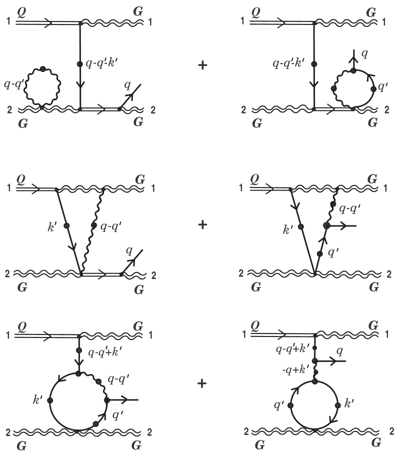
Figure 11: Some of soft one-loop corrections to soft quark bremsstrahlung process depicted in Fig.2.

In the approximation of the static color center model in (8.14) one can drop all the contributions proportional to $(\bar{\chi}_{2}u(\hat{\bf q},\lambda))$ and $(\bar{\chi}_{2}v(\hat{\bf q},\lambda))$. Further, we substitute (8.14) into the formula for radiation intensity (3.5) and perform the average over the transverse impact parameter ${\bf b}$. As a result we arrive at the following expression of the ‘off-diagonal’ energy losses for the first term on the right-hand side of Eq. (8.14)

$$\left(\!-\frac{dE_{1}}{dx}\right)_{\!{\rm off-diag}}=\check{\Lambda}_{1}+\check{\Lambda}_{2},$$

where

$$\check{\Lambda}_{1}=-2\biggl{(}\frac{{\alpha}_{s}}{\pi}\biggr{)}^{\!3}\!\!\sum\limits_{\,\zeta=Q,\,\bar{Q}}\!\!C_{\theta\theta}^{(1;\zeta)}\!\!\int\!{\bf p}_{2}^{2}\left[f_{|{\bf p}_{2}|}^{(\zeta)}+f_{|{\bf p}_{2}|}^{(G)}\right]\frac{d|\,{\bf p}_{2}|}{2\pi^{2}}$$ (8.15)

$$\times\!\sum\limits_{\lambda\,=\,\pm}\int\!d{\bf q}dq^{0}\,q^{0}\,{\rm Im}\,(\!\,^{\ast}\!\Delta_{+}(q))\,\delta(v_{1}\cdot q)\int\!d{\bf q}^{\prime}\,\Biggl{(}{\rm Re}\,\beta_{1}\,\frac{|[\bar{\chi}_{1}u(\hat{\bf q},\lambda)]|^{\,2}}{({\bf v}_{1}\cdot{\bf q}^{\prime})^{2}}\left|\left[\bar{\chi}_{1}\!\,^{\ast}\!S(q^{\prime})\chi_{2}\right]\right|^{\,2}$$

$$-\frac{1}{({\bf v}_{1}\!\cdot\!{\bf q}^{\prime})}\,{\rm Re}\Bigl{\{}[\bar{\chi}_{1}u(\hat{\bf q},\lambda)]\!\left[\bar{\chi}_{2}\!\,^{\ast}\!S(-q^{\prime})\chi_{1}\right]\![\bar{u}(\hat{\bf q},\lambda)\!\,^{\ast}\Gamma^{(Q)}_{\mu}(q-q^{\prime};q^{\prime},-q)\!\,^{\ast}\!S(q^{\prime})\chi_{\!2}]\!\,^{\ast}{\cal D}^{\mu\nu}_{C}\!(q-q^{\prime})v_{1\nu^{\prime}}\!\Bigr{\}}\!\!\Biggr{)}_{\!\!\!q_{0}^{\prime}=0}$$

$$+\;\Bigl{(}\,^{\ast}{\!\Delta}_{+}(q)\rightarrow\,^{\ast}{\!\Delta}_{-}(q),\;u(\hat{\bf q},\lambda)\rightarrow v(\hat{\bf q},\lambda)\Bigr{)},$$

and

$$\check{\Lambda}_{2}=2\biggl{(}\frac{{\alpha}_{s}}{\pi}\biggr{)}^{\!3}\!\!\sum\limits_{\,\zeta=Q,\,\bar{Q}}\!\!C_{\theta\theta}^{(1;\zeta)}\!\!\int\!{\bf p}_{2}^{2}\left[f_{|{\bf p}_{2}|}^{(\zeta)}+f_{|{\bf p}_{2}|}^{(G)}\right]\frac{d|\,{\bf p}_{2}|}{2\pi^{2}}$$ (8.16)

$$\times\!\sum\limits_{\lambda\,=\,\pm}\int\!d{\bf q}dq^{0}\,q^{0}\,{\rm Im}\,(\!\,^{\ast}\!\Delta_{+}(q))\,\delta(v_{1}\cdot q)\!\int\!d{\bf q}^{\prime}$$

$$\times{\rm Re}\Bigl{\{}[\bar{\chi}_{1}u(\hat{\bf q},\lambda)](\bar{\chi}_{2}\!\,^{\ast}\!S(-q^{\prime}))_{{\alpha}_{\!1}}\!\Bigl{[}\,\bar{u}_{\alpha}(\hat{\bf q},\lambda)M_{\alpha\alpha_{1}\alpha_{2}\beta}(-q,-q;q^{\prime},q^{\prime})(\!\,^{\ast}\!S(q)\chi_{\!1})_{\beta})\Bigr{]}(\!\,^{\ast}\!S(q^{\prime})\chi_{\!2})_{\alpha_{2}}\!\Bigr{\}}_{\!q_{0}^{\prime}=0}$$

$$+\;\Bigl{(}\,^{\ast}{\!\Delta}_{+}(q)\rightarrow\,^{\ast}{\!\Delta}_{-}(q),\;u(\hat{\bf q},\lambda)\rightarrow v(\hat{\bf q},\lambda)\Bigr{)}.$$

In the last expression we have used the definition of the $M_{\alpha\alpha_{1}\alpha_{2}\beta}$ function:

$$M_{\alpha\alpha_{1}\alpha_{2}\beta}(-q,-q;q^{\prime},q^{\prime})=\!\,^{\ast}\Gamma^{(Q)\mu}_{\alpha\alpha_{2}}(q-q^{\prime};q^{\prime},-q)\,^{\ast}{\cal D}_{\mu\nu}(q-q^{\prime})\!\,^{\ast}\Gamma^{(Q)\nu}_{\alpha_{1}\beta}(q-q^{\prime};q^{\prime},-q).$$

It was introduced in Paper I (section 6). The given function appears in the elastic scattering amplitude of soft fermionic excitations off each other. The diagrammatic interpretation of different terms in $\check{\Lambda}_{1}$ and $\check{\Lambda}_{2}$ is presented in Fig. 12. There two cases are considered: when the initial parton 1 is a hard quark and final parton is a hard gluon and vice versa. In so doing in the former case (virtual) soft-quark excitation is radiated and in the latter case soft-antiquark excitation is.

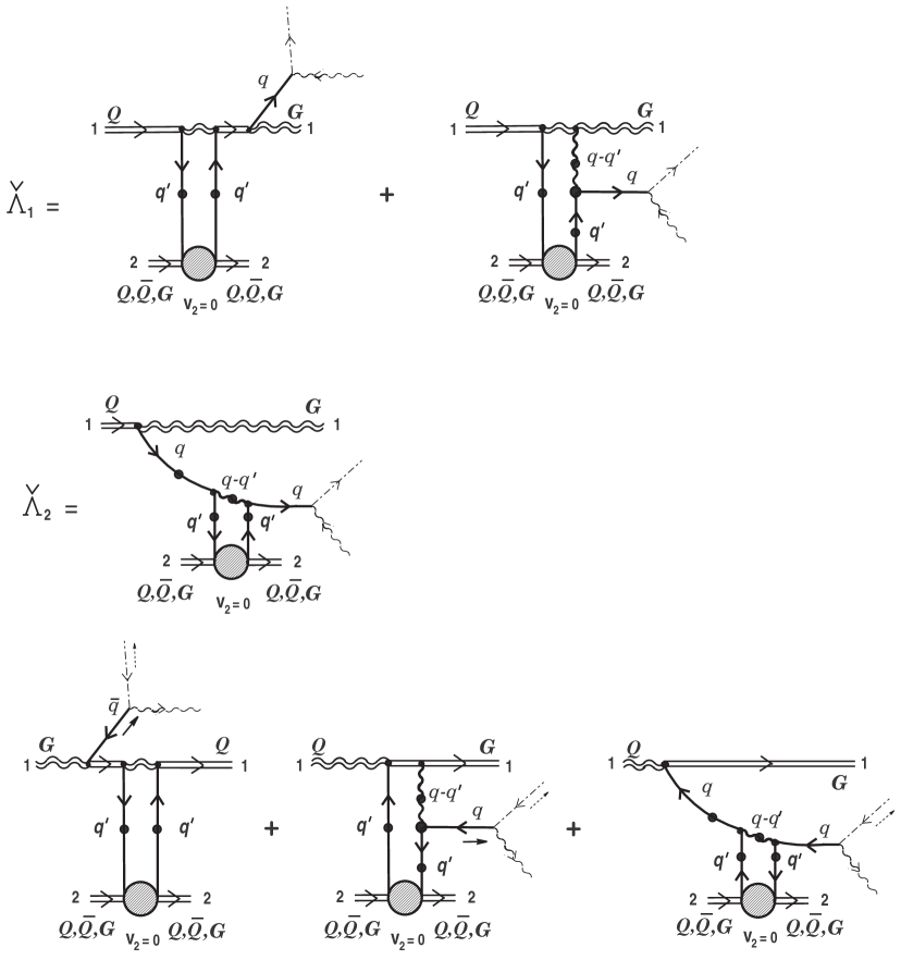
Figure 12: The second, additional to figure 10, part of the ‘off-diagonal’ contributions to soft-quark radiation energy losses.

Let us consider now a contribution to the ‘off-diagonal’ energy losses of the second term on the right-hand side of Eq. (8.14). By the same arguments, we obtain

$$\left(\!-\frac{dE_{1}}{dx}\right)_{\!{\rm off-diag}}=-2\,\biggl{(}\frac{{\alpha}_{s}}{\pi}\biggr{)}^{\!3}\!\!\!\sum\limits_{\,\zeta=Q,\,\bar{Q}}\!\!\tilde{C}_{\theta\theta}^{(1;\,\zeta)}\!\!\int\!{\bf p}_{2}^{2}\left[f_{|{\bf p}_{2}|}^{(\zeta)}+f_{|{\bf p}_{2}|}^{(G)}\right]\frac{d|\,{\bf p}_{2}|}{2\pi^{2}}$$ (8.17)

$$\times\!\sum\limits_{\lambda\,=\,\pm}\int\!d{\bf q}dq^{0}\,q^{0}\,{\rm Im}\,(\!\,^{\ast}\!\Delta_{+}(q))\,\delta(v_{1}\cdot q)\int\!d{\bf q}^{\prime}\,\Biggl{[}{\rm Re}\,\beta\,\frac{|[\bar{\chi}_{1}u(\hat{\bf q},\lambda)]|^{\,2}}{({\bf v}_{1}\cdot{\bf q}^{\prime})^{2}}\left|\left[\bar{\chi}_{1}\!\,^{\ast}\!S(q^{\prime})\chi_{2}\right]\right|^{\,2}$$

$$+\,{\rm Re}\biggl{\{}\biggl{(}\frac{v_{1\mu}}{(v_{1}\cdot q)}\,[\bar{u}(\hat{\bf q},\lambda)\chi_{1}]-[\bar{u}(\hat{\bf q},\lambda)\!\,^{\ast}\Gamma^{(Q)}_{\mu}(0;q,-q)\!\,^{\ast}\!S(q)\chi_{\!1}]\biggr{)}\,^{\ast}{\cal D}^{\mu\nu}_{C}\!(0)\hskip 85.35826pt$$

$$\hskip 227.62204pt\times\,[\bar{\chi}_{2}\!\,^{\ast}\!S(-q^{\prime})\!\,^{\ast}\Gamma^{(G)}_{\nu}(0;q^{\prime},-q^{\prime})\!\,^{\ast}\!S(q^{\prime})\chi_{\!2}]\biggl{\}}\!\Biggr{]}_{q_{0}^{\prime}=0}$$

$$+\;\Bigl{(}\,^{\ast}{\!\Delta}_{+}(q)\rightarrow\,^{\ast}{\!\Delta}_{-}(q),\;u(\hat{\bf q},\lambda)\rightarrow v(\hat{\bf q},\lambda)\Bigr{)}.$$

Unlike two previous pairs of equations (8.6), (8.7) and (8.15), (8.16) the situation here becomes less clear from the standpoint of physical interpretation. The main reason of this is appearance of the resummed gluon propagator $\,{}^{\ast}{\cal D}^{\mu\nu}_{C}\!(0)$ for the zeroth momentum transfer. For the components $\mu=\nu=0$ we can formally use the expression $\,{}^{\ast}{\cal D}_{C}^{00}(0)=1/\mu_{D}^{2}$, whereas the ‘transverse’ part ${}^{\ast}{\cal D}_{C}^{ij}(0)$ is singular. Diagrammatic interpretation of the terms with $\,{}^{\ast}{\cal D}_{C}^{00}(0)$ is presented in Fig. 13.

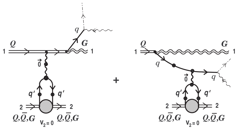
Figure 13: The contact double Born graphs in which an intermediate virtual gluon has zeroth four-momentum.

The contribution to the ‘off-diagonal’ energy losses of the last effective source (8.10) is still less clear from the physical point of view. Making use (6.10), we define in the first place an explicit form of the coefficient functions entering into definition (8.10). So first of them has the following structure:

$$K_{\alpha}^{(II)\,ij,kl}({\bf v}_{1},{\bf v}_{2};\,\ldots|\,q)$$

$$=\frac{g^{5}}{(2\pi)^{9}}\,\Bigl{[}(t^{a})^{ik}(t^{a})^{jl}-(t^{a})^{i\,l}(t^{a})^{jk}\Bigr{]}K_{\alpha}^{(II)}({\bf v}_{1},{\bf v}_{2};\,\ldots|\,q),$$

where

$$K_{\alpha}^{(II)}({\bf v}_{1},{\bf v}_{2};\,\ldots|\,q)$$

$$=\int\!\biggl{\{}K^{(Q)}_{\alpha\mu}({\bf v}_{2},\chi_{2}|\,q-q^{\prime},-q)\,^{\ast}{\cal D}^{\mu\nu}(q-q^{\prime})[\,\bar{\chi}_{1\,}{\cal K}_{\nu}({\bf v}_{1},{\bf v}_{2}|\,q-q^{\prime},-k^{\prime})\chi_{2}]$$

$$-\,(\beta-\beta_{1})\,\frac{\chi_{2\alpha}}{(v_{2}\cdot(q-q^{\prime}-k^{\prime}))(v_{2}\cdot q^{\prime})}\,\left[\,\bar{\chi}_{2}\,^{\ast}\!S(q^{\prime})\chi_{2}\right]\left[\,\bar{\chi}_{1}\,^{\ast}\!S(q-q^{\prime}-k^{\prime})\chi_{2}\right]$$

$$-\,\tilde{\beta}_{1}\,\frac{\chi_{1\alpha}}{(v_{2}\cdot k^{\prime})(v_{2}\cdot q^{\prime})}\,\left[\,\bar{\chi}_{1}\,^{\ast}\!S(k^{\prime})\chi_{2}\right]\left[\,\bar{\chi}_{1}\,^{\ast}\!S(q^{\prime})\chi_{2}\right]\biggr{\}}$$ (8.18)

$$\times\,{\rm e}^{-i({\bf q}-{\bf q}^{\prime}-{\bf k}^{\prime})\cdot\,{\bf x}_{01}}\,{\rm e}^{-i({\bf q}^{\prime}+{\bf k}^{\prime})\cdot\,{\bf x}_{02}}\,\delta(v_{1}\cdot(q-q^{\prime}-k^{\prime}))\,\delta(v_{2}\cdot k^{\prime})\delta(v_{2}\cdot q^{\prime})\,dk^{\prime}dq^{\prime}.$$

By virtue of the color structure, the coefficient function is automatically anti-symmetric with respect to the replacement $k\rightleftharpoons l$ as it should be.

Let us analyze just in detail a general form of effective sources (8.8) and (8.10). In effective source (8.8) we have in the first and second terms the bunches $\theta_{01}^{\dagger j}\theta_{01}^{k}$ and $\theta_{02}^{\dagger j}\theta_{02}^{k}$, respectively. As was already discussed above presence of such the “bunches” point to the fact that statistics of the first (second) hard particle does not change in the process of interaction generated by the effective source under consideration (although it can change in an internal virtual line). In effective source (8.10) we have in turn the bunches $\theta_{01}^{k}\theta_{01}^{l}$ and $\theta_{02}^{k}\theta_{02}^{l}$, correspondingly. Here the following interpretation is relevant: as above the statistics of the first (second) hard particle in the process of interaction induced by the effective source in question also does not change. Meanwhile, the changing from a hard quark $Q$ to a hard antiquark $\bar{Q}$ and conversely are taking place. In Fig. 14 a possible diagrammatic interpretation of some terms of function (8.18) is given. As a hard parton 1 here we take a hard antiquark and as a initial hard parton 2 do a hard quark.

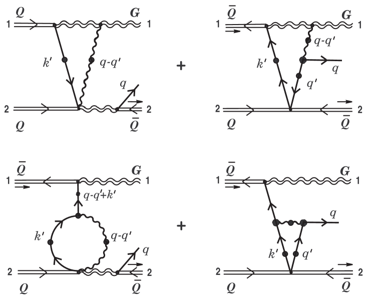
Figure 14: Some of soft one-loop corrections to bremsstrahlung process of a soft quark, in which one of hard half-spin particles (in this case particle 2) changes to antiparticle.

Now we written out an expression for the ‘off-diagonal’ energy losses in the static limit induced by effective source (8.10), (8.18). One also presents this expression in the form of the sum of two parts

$$\left(\!-\frac{dE_{1}}{dx}\right)_{\!{\rm off-diag}}^{\!t}=\tilde{\Lambda}_{1}+\tilde{\Lambda}_{2},$$

where

$$\tilde{\Lambda}_{1}=-\biggl{(}\frac{{\alpha}_{s}}{\pi}\biggr{)}^{\!3}\Biggl{(}\sum\limits_{\,\zeta=Q,\,\bar{Q}\,}\!\int\!{\bf p}_{2}^{2}\left[f_{|{\bf p}_{2}|}^{(\zeta)}+f_{|{\bf p}_{2}|}^{(G)}\right]\frac{d|\,{\bf p}_{2}|}{2\pi^{2}}\Biggr{)}\!\sum\limits_{\lambda\,=\,\pm}\int\!d{\bf q}dq^{0}\,q^{0}\,{\rm Im}\,(\!\,^{\ast}\!\Delta_{+}(q))\,\delta(v_{1}\cdot q)$$ (8.19)

$$\times\!\int\!d{\bf q}^{\prime}\,{\rm Re}\Biggl{\{}[\theta_{01}^{\dagger i}(t^{a})^{ik}\theta_{02}^{k}]^{2}\Biggl{[}\,\tilde{\beta}_{1}\,\frac{|[\bar{\chi}_{1}u(\hat{\bf q},\lambda)]|^{\,2}}{({\bf v}_{1}\cdot{\bf q}^{\prime})^{2}}\left[\bar{\chi}_{1}\!\,^{\ast}\!S(-q^{\prime})\chi_{2}\right]\left[\bar{\chi}_{1}\!\,^{\ast}\!S(q^{\prime})\chi_{2}\right]$$

$$-\frac{1}{({\bf v}_{1}\!\cdot\!{\bf q}^{\prime})}\,[\bar{\chi}_{1}u(\hat{\bf q},\lambda)]\!\left[\bar{\chi}_{1}\!\,^{\ast}\!S(-q^{\prime})\chi_{2}\right]\![\bar{u}(\hat{\bf q},\lambda)\!\,^{\ast}\Gamma^{(Q)}_{\mu}(q-q^{\prime};q^{\prime},-q)\!\,^{\ast}\!S(q^{\prime})\chi_{\!2}]\!\,^{\ast}{\cal D}^{\mu\nu}\!(q-q^{\prime})v_{1\nu}\!\Biggr{]}\!\Biggr{\}}_{\!q_{0}^{\prime}=0}$$

$$+\;\Bigl{(}\,^{\ast}{\!\Delta}_{+}(q)\rightarrow\,^{\ast}{\!\Delta}_{-}(q),\;u(\hat{\bf q},\lambda)\rightarrow v(\hat{\bf q},\lambda)\Bigr{)}$$

and

$$\tilde{\Lambda}_{2}=\biggl{(}\frac{{\alpha}_{s}}{\pi}\biggr{)}^{\!3}\Biggl{(}\sum\limits_{\,\zeta=Q,\,\bar{Q}\,}\!\int\!{\bf p}_{2}^{2}\left[f_{|{\bf p}_{2}|}^{(\zeta)}+f_{|{\bf p}_{2}|}^{(G)}\right]\frac{d|\,{\bf p}_{2}|}{2\pi^{2}}\Biggr{)}$$ (8.20)

$$\times\sum\limits_{\lambda\,=\,\pm}\int\!d{\bf q}dq^{0}\,q^{0}\,{\rm Im}\,(\!\,^{\ast}\!\Delta_{+}(q))\,\delta(v_{1}\cdot q)\int\!d{\bf q}^{\prime}\,{\rm Re}\biggl{\{}[\theta_{01}^{\dagger i}(t^{a})^{ik}\theta_{02}^{k}]^{2}\,[\bar{\chi}_{1}u(\hat{\bf q},\lambda)]$$

$$\times\,\!\Bigl{[}\,\bar{u}_{\alpha}(\hat{\bf q},\lambda)(\bar{\chi}_{1}\!\,^{\ast}\!S(q))_{\beta}M_{\alpha\beta\alpha_{1}\alpha_{2}}(-q,-q;q^{\prime},q^{\prime})(\!\,^{\ast}\!S(q^{\prime})\chi_{\!2})_{\alpha_{1}}\,(\!\,^{\ast}\!S(-q^{\prime})\chi_{\!2})_{\alpha_{2}}\Bigr{]}\!\biggr{\}}_{\!q_{0}^{\prime}=0}$$

$$+\;\Bigl{(}\,^{\ast}{\!\Delta}_{+}(q)\rightarrow\,^{\ast}{\!\Delta}_{-}(q),\;u(\hat{\bf q},\lambda)\rightarrow v(\hat{\bf q},\lambda)\Bigr{)}.$$

In comparison with (8.15), (8.16), and (8.17) it is already impossible to take the color factor $[\theta_{01}^{\dagger i}(t^{a})^{ik}\theta_{02}^{k}]^{2}$ outside the real part sign in the above equations. Under the conjugation it does not transform into itself (as in the case of $[\theta_{01}^{\dagger i}(t^{a})^{ik}\theta_{02}^{k}][\theta_{02}^{\dagger j}(t^{a})^{jl}\theta_{01}^{l}]$ and $[\theta_{01}^{\dagger i}(t^{a})^{ik}\theta_{01}^{k}][\theta_{02}^{\dagger j}(t^{a})^{jl}\theta_{02}^{l}]$). It is not clear whether it is possible to identify this factor with some (complex) number in general. In Fig. 15 we give graphic illustration of plausible bremsstrahlung processes defined by the $\tilde{\Lambda}_{1}$ and $\tilde{\Lambda}_{2}$ functions.

Figure 15: The diagrammatic interpretation of terms entering into the ‘off-diagonal’ energy losses (8.19), (8.20).

9 Cancellation of singularities in soft-quark bremsstrahlung

Let us analyze a role of the ‘off-diagonal’ energy losses obtained in the previous section. First we consider the contributions $\hat{\Lambda}_{1}$ (8.6), $\check{\Lambda}_{1}$ (8.15) and the first term in (8.17) (we neglect the contribution $\tilde{\Lambda}_{1}$, Eq. (8.19), as physically less evident). The given functions for the off-shell soft excitations contain singularities of the type: $1/({\bf v}_{1}\cdot{\bf q}^{\prime})^{2}$ and $1/({\bf v}_{1}\cdot{\bf q}^{\prime})$. As well as in section 7 we require that these singularities in accuracy should be cancelled by corresponding ones which contain in the main ‘diagonal’ contribution (3.10). Setting ${\bf v}_{2}=0$ and dropping the terms proportional to $[\bar{\chi}_{2}u(\hat{\bf q},\lambda)]$ and $[\bar{\chi}_{2}v(\hat{\bf q},\lambda)]$, we rewrite this ‘diagonal’ contribution once more, considered the module squared $|\,\bar{u}(\hat{\bf q},\lambda){\cal K}\,|^{\,2}$

$$\left(\!-\frac{dE_{1}}{dx}\right)_{\!{\rm diag}}=\biggl{(}\frac{{\alpha}_{s}}{\pi}\biggr{)}^{\!3}\Biggl{(}\frac{C_{F}\,C_{2}^{(1)}}{d_{A}}\Biggr{)}\!\!\sum\limits_{\,\zeta=Q,\,\bar{Q}}\!\!C_{\theta}^{(\zeta)}\!\!\int\!{\bf p}_{2}^{2}\left[f_{|{\bf p}_{2}|}^{(\zeta)}+f_{|{\bf p}_{2}|}^{(G)}\right]\frac{d|\,{\bf p}_{2}|}{2\pi^{2}}$$ (9.1)

$$\times\!\sum\limits_{\lambda\,=\,\pm}\int\!d{\bf q}dq^{0}\,q^{0}\,{\rm Im}\,(\!\,^{\ast}\!\Delta_{+}(q))\int\!d{\bf q}^{\prime}\,\Biggl{\{}\alpha^{2}\,\frac{|\,[\bar{\chi}_{1}u(\hat{\bf q},\lambda)]|^{\,2}}{({\bf v}_{1}\cdot{\bf q}^{\prime})^{2}}\left|\,\left[\bar{\chi}_{1}\!\,^{\ast}\!S(q^{\prime})\chi_{2}\right]\right|^{\,2}$$

$$-2\frac{\alpha}{({\bf v}_{1}\!\cdot\!{\bf q}^{\prime})}\,{\rm Re}\Bigl{\{}[\bar{\chi}_{1}u(\hat{\bf q},\lambda)]\!\left[\bar{\chi}_{2}\!\,^{\ast}\!S(-q^{\prime})\chi_{1}\right]\![\bar{u}(\hat{\bf q},\lambda)\!\,^{\ast}\Gamma^{(Q)}_{\mu}(q-q^{\prime};q^{\prime},-q)\!\,^{\ast}\!S(q^{\prime})\chi_{\!2}]\!\,^{\ast}{\cal D}^{\mu\nu}\!(q-q^{\prime})v_{1\nu}\!\Bigr{\}}$$

$$+\,\Bigl{|}\,[\bar{u}(\hat{\bf q},\lambda)\!\,^{\ast}\Gamma^{(Q)}_{\mu}(q-q^{\prime};q^{\prime},-q)\!\,^{\ast}\!S(q^{\prime})\chi_{\!2}]\,^{\ast}{\cal D}^{\mu\nu}\!(q-q^{\prime})v_{1\nu}\Bigr{|}^{\,2}\Biggr{\}}_{q_{0}^{\prime}=0}\delta(v_{1}\cdot q+{\bf v}_{1}\cdot{\bf q}^{\prime})$$

$$+\,\biggl{(}\frac{{\alpha}_{s}}{\pi}\biggr{)}^{\!3}\Biggl{(}\frac{C_{F}\,C_{\theta}^{(1)}}{d_{A}}\Biggr{)}\sum\limits_{\,\zeta=Q,\,\bar{Q},\,G}\!\!C_{2}^{(\zeta)}\!\!\int\!{\bf p}_{2}^{2}\,f_{|{\bf p}_{2}|}^{(\zeta)}\,\frac{d|\,{\bf p}_{2}|}{2\pi^{2}}$$

$$\times\sum\limits_{\lambda\,=\,\pm}\int\!d{\bf q}dq^{0}\,q^{0}\,{\rm Im}\,(\!\,^{\ast}\!\Delta_{+}(q))\int\!d{\bf q}^{\prime}\,\frac{1}{({\bf q}^{\prime\,2}+\mu_{D}^{2})^{2}}\,\Biggl{\{}\frac{|\,[\bar{\chi}_{1}u(\hat{\bf q},\lambda)]|^{\,2}}{({\bf v}_{1}\cdot{\bf q}^{\prime})^{2}}$$

$$+\,2\,\frac{1}{({\bf v}_{1}\!\cdot\!{\bf q}^{\prime})}\,{\rm Re}\,\Bigl{\{}[\bar{\chi}_{1}u(\hat{\bf q},\lambda)][\bar{u}(\hat{\bf q},\lambda)\!\,^{\ast}\Gamma^{(Q)0}(q^{\prime};q-q^{\prime},-q)\!\,^{\ast}\!S(q-q^{\prime})\chi_{\!1}]\Bigr{\}}$$

$$+\,\Bigl{|}\,[\bar{u}(\hat{\bf q},\lambda)\!\,^{\ast}\Gamma^{(Q)0}(q^{\prime};q-q^{\prime},-q)\!\,^{\ast}\!S(q-q^{\prime})\chi_{\!1}]\Bigr{|}^{\,2}\Biggr{\}}_{q_{0}^{\prime}=0}\delta(v_{1}\cdot q+{\bf v}_{1}\cdot{\bf q}^{\prime})$$

$$+\;\Bigl{(}\,^{\ast}{\!\Delta}_{+}(q)\rightarrow\,^{\ast}{\!\Delta}_{-}(q),\;u(\hat{\bf q},\lambda)\rightarrow v(\hat{\bf q},\lambda)\Bigr{)}.$$

The contribution $\hat{\Lambda}_{1}$ is the most simple for an analysis. This contribution should be compared with the last term proportional to the second order Casimir $C_{2}^{(\zeta)},\,\zeta=Q,\bar{Q},G$ in the above equation. It can be easily checked that in the limit $({\bf v}_{1}\cdot{\bf q}^{\prime})\rightarrow 0$ the singular terms $1/({\bf v}_{1}\cdot{\bf q}^{\prime})^{2}$ and $1/({\bf v}_{1}\cdot{\bf q}^{\prime})$ in the $\hat{\Lambda}_{1}$ function and in the term just mentioned exactly cancel each other. Further, it is necessary to confront the first term in the ‘diagonal’ energy losses (9.1) (proportional to the constant $C_{\theta}^{(\zeta)},\,\zeta=Q,\,\bar{Q}$) with the sum of two functions $\check{\Lambda}_{1}$ (8.15) and the first term in the integrand of (8.17). The latter contains the singularity $1/({\bf v}_{1}\cdot{\bf q}^{\prime})^{2}$ multiplied by the constant ${\rm Re}\,\beta$. The requirement of cancellation of the singularities gives rise to the following system of equations:

$$C_{\theta\theta}^{(1;\,\zeta)}{\rm Re}\,\beta_{1}\,+\,\tilde{C}_{\theta\theta}^{(1;\,\zeta)}{\rm Re}\,\beta=\frac{1}{2}\,\alpha^{2}\Biggl{(}\frac{C_{F}\,C_{2}^{(1)}}{d_{A}}\Biggr{)}C_{\theta}^{(\zeta)},$$

$$C_{\theta\theta}^{(1;\,\zeta)}=\Biggl{(}\frac{C_{F}\,C_{2}^{(1)}}{d_{A}}\Biggr{)}C_{\theta}^{(\zeta)}\alpha.$$

The second equation here coincides with the first one in a system of equations (7.14). The first equation can be viewed as the definition of the color factor $\tilde{C}^{(1;\xi)}_{\theta\theta}$.

Now we proceed to an interpretation of the functions $\hat{\Lambda}_{2}$ (8.7) and $\check{\Lambda}_{2}$ (8.16). Here we will follow the way outlined in section 7. It will be shown that these functions can be partly interpreted as those taking into account a change of dispersion properties of the medium caused by the processes of nonlinear interaction of soft collective excitations. For this purpose we make use the expression for the polarization energy losses of a fast parton 1 (II.10.3). In this expression we replace the quark propagator in the HTL-approximation $\!\,{}^{\ast}\!S(q^{\prime})$ by the effective one $\!\,{}^{\ast}\!\tilde{S}(q^{\prime})$ considering a change of dispersion properties of the QGP induced by nonlinear dynamics of soft excitations:

$$\left(\!-\frac{dE_{1}}{dx}\right)=\biggl{(}\frac{\alpha_{s}}{2{\pi}^{2}}\biggr{)}\,C_{\theta}^{(1)}\!\!\int\!d{\bf q}dq^{0}q^{0}\,{\rm Im}\left(\bar{\chi}_{1}\,^{\ast}\!\tilde{S}(q)\chi_{1}\right)\delta(v_{1}\cdot q).$$ (9.2)

Let us take the effective quark propagator $\,{}^{\ast}\!\tilde{S}(q)$ in a linear approximation in the spectral densities

$$\,{}^{\ast}\!\tilde{S}(q)\,\simeq\,^{\ast}\!{S}(q)\,+\,^{\ast}\!{S}(q)\Sigma^{(1)}[\,\Upsilon,\,I\,](q)\,^{\ast}\!{S}(q)\,+\ldots\,.$$

Further, we use representation (II.11.9) for an imaginary part in the integrand in (9.2)

$${\rm Im}\!\left(\bar{\chi}_{1}\,^{\ast}\!\tilde{S}(q)\chi_{1}\right)\simeq{\rm Im}\left(\,{}^{\ast}{\!\Delta}_{+}(q)\right)\!\sum\limits_{\lambda,\,\lambda^{\prime}=\,\pm}\!\biggl{(}\,\delta^{\lambda\lambda^{\prime}}[\bar{u}(\hat{\bf q},\lambda^{\prime})\chi_{1}][\bar{\chi}_{1}u(\hat{\bf q},\lambda)]$$ (9.3)

$$+\,{\rm Re}\,\Bigl{\{}[\bar{u}(\hat{\bf q},\lambda^{\prime})\chi_{1}][\bar{\chi}_{1}u(\hat{\bf q},\lambda)]\,\Sigma^{(1)}_{++}(q;\lambda,\lambda^{\prime})\,^{\ast}\!\Delta_{+}(q)\Bigr{\}}$$

$$\hskip 2.84544pt+\,{\rm Re}\,\Bigl{\{}[\bar{v}(\hat{\bf q},\lambda^{\prime})\chi_{1}][\bar{\chi_{1}}u(\hat{\bf q},\lambda)]\Sigma^{(1)}_{+-}(q;\lambda,\lambda^{\prime})\,^{\ast}\!\Delta_{-}(q)\Bigr{\}}\!\biggr{)}$$

$$+\,{\rm Re}\left(\,{}^{\ast}{\!\Delta}_{+}(q)\right)\!\sum\limits_{\lambda,\,\lambda^{\prime}=\,\pm}\!\biggl{(}{\rm Im}\,\Bigl{\{}[\bar{u}(\hat{\bf q},\lambda^{\prime})\chi_{1}][\bar{\chi}_{1}u(\hat{\bf q},\lambda)]\,\Sigma^{(1)}_{++}(q;\lambda,\lambda^{\prime})\,^{\ast}\!\Delta_{+}(q)\Bigr{\}}$$

$$\hskip 102.43008pt+\,{\rm Im}\,\Bigl{\{}[\bar{v}(\hat{\bf q},\lambda^{\prime})\chi_{1}][\bar{\chi}_{1}u(\hat{\bf q},\lambda)]\,\Sigma^{(1)}_{+-}(q;\lambda,\lambda^{\prime})\,^{\ast}\!\Delta_{-}(q)\Bigr{\}}\!\biggr{)}$$

$$\hskip 39.83368pt+\,\Bigr{(}\,^{\ast}{\!\Delta}_{\pm}(q)\rightleftharpoons\,^{\ast}{\!\Delta}_{\mp}(q),\,u(\hat{\bf q},\lambda)\rightleftharpoons v(\hat{\bf q},\lambda),\,u(\hat{\bf q},\lambda^{\prime})\rightleftharpoons v(\hat{\bf q},\lambda^{\prime}),\,\ldots\Bigr{)}.$$

Here,

$$\Sigma_{++}^{(1)}(q;\lambda,\lambda^{\prime})\equiv[\bar{u}(\hat{\bf q},\lambda)\Sigma^{(1)}(q)u(\hat{\bf q},\lambda^{\prime})]$$ (9.4)

$$=2g^{2}\,C_{F}\!\int\!dq^{\prime}\,\Upsilon_{\alpha_{2}\alpha_{1}}(q^{\prime})\Bigl{[}\,\bar{u}_{\alpha}(\hat{\bf q},\lambda)\,{\rm M}_{\alpha\alpha_{1}\alpha_{2}\beta}(-q,-q;q^{\prime},q^{\prime})u_{\beta}(\hat{\bf q},\lambda^{\prime})\Bigr{]}$$

$$-\,g^{2}C_{F}\!\int\!dk^{\prime}\,I_{\mu\nu}(k^{\prime})\Bigl{[}\,\bar{u}_{\alpha}(\hat{\bf q},\lambda){\cal T}^{({Q;\,\cal S})\mu\nu}_{\alpha\beta}\!(k^{\prime},-k^{\prime};q,-q)u_{\beta}(\hat{\bf q},\lambda^{\prime})\Bigr{]}\hskip 5.69046pt$$

and so on. In deriving (9.3) we have used the expansion of the HTL-resummed quark propagator

$${}^{\ast}\!S_{\beta\beta^{\prime}}(q)=\sum\limits_{\lambda^{\prime}=\pm}\Bigl{\{}[\,u_{\beta}(\hat{\bf q},\lambda^{\prime})\bar{u}_{\beta^{\prime}}(\hat{\bf q},\lambda^{\prime})]\,^{\ast}\!\Delta_{+}(q)+[\,v_{\beta}(\hat{\bf q},\lambda^{\prime})\bar{v}_{\beta^{\prime}}(\hat{\bf q},\lambda^{\prime})]\,^{\ast}\!\Delta_{-}(q)\Bigr{\}}.$$ (9.5)

Let us substitute the quark spectral density (7.19) into the first term on the right-most side of Eq. (9.4) (the same is also true for the functions $\Sigma_{+-}^{(1)},\,\Sigma_{-\,+}^{(1)}$, and $\Sigma_{--}^{(1)}$). It is easily to see that the correction terms in (9.2) proportional to ${\rm Im}\,^{\ast}{\!\Delta}_{\pm}(q)$, exactly reproduce the function $\check{\Lambda}_{2}$ if one takes into account conditions for cancellation of the singularities (7.14), value for the constant $\alpha:\,\alpha=-C_{F}/T_{F}$, and the relation

$$n_{f}T_{F}=N_{c}.$$

As it was pointed in Paper II this relation is fulfilled for $n_{f}=6,\,T_{F}=1/2$, and $N_{c}=3$, i.e. at extremely high temperatures of the system under consideration when we can neglect mass of all quark flavors.

Further, we consider the second term on the right-hand side of Eq. (9.4). Let us derive an explicit form of the soft-gluon spectral density $I_{\mu\nu}(k^{\prime})$. Here we proceed in just the same way as in section 7 in determining the soft-quark spectral density. The initial definition of the soft-gluon spectral density is

$$\left\langle A_{\mu}^{\ast a}(k^{\prime})A_{\nu}^{b}(k_{1})\right\rangle=\delta^{ab}I_{\mu\nu}(k^{\prime})\,\delta(k^{\prime}-k_{1}).$$

For the problem in question soft gluon field $A_{\mu}^{a}$ is induced by a hard test particle 2 (which is located at the position ${\bf x}_{02}$) and thus

$$A^{a\mu}(k;{\bf x}_{02})=-\!\,^{\ast}{\cal D}^{\mu\mu^{\prime}}_{C}(k)j_{Q_{2}\mu^{\prime}}^{(0)a}(k;{\bf x}_{02}),$$ (9.6)

where

$$j_{Q_{2}\mu^{\prime}}^{(0)a}(k;{\bf x}_{02})=\frac{\,g}{(2\pi)^{3}}\;v_{2\mu^{\prime}}Q_{02}^{a}\,\delta(v_{2}\cdot k)\,{\rm e}^{-i{\bf k}\cdot\,{\bf x}_{02}}\,.$$

As an definition of the soft-gluon spectral density we take the following expression

$$I_{\mu\nu}(k^{\prime})=\frac{1}{d_{A}}\!\sum\limits_{\;\zeta=Q,\,\bar{Q},\,G\,}\!\int\!{\bf p}_{2}^{2}\,f_{|{\bf p}_{2}|}^{(\zeta)}\,\frac{d|\,{\bf p}_{2}|}{2\pi^{2}}\int\!\frac{d\Omega_{{\bf v}_{2}}}{4\pi}\int\!d{\bf x}_{02}\int\!dk_{1}\left\langle A_{\mu}^{\ast(0)a}(k^{\prime};{\bf x}_{02})A_{\nu}^{(0)b}(k_{1};{\bf x}_{02})\right\rangle\,.$$

In the static limit $({\bf v}_{2}=0)$ we are only interested in the spectral density $I_{00}(k^{\prime})$. Substituting (9.6) into the foregoing expression we get in the limit being considered

$$I_{00}(k_{0}^{\prime},{\bf k}^{\prime})=\frac{g^{2}}{(2\pi)^{3}}\,\frac{1}{d_{A}}\Biggl{(}\sum\limits_{\;\zeta=Q,\,\bar{Q},\,G\,}\!\!\!\!C_{2}^{(\zeta)}\!\!\int\!{\bf p}_{2}^{2}\,f_{|{\bf p}_{2}|}^{(\zeta)}\,\frac{d|\,{\bf p}_{2}|}{2\pi^{2}}\,\Biggr{)}\frac{1}{({\bf k}^{\,\prime 2}+\mu_{D}^{2})^{2}}\;\delta(k_{0}^{\prime}).$$ (9.7)

Further, substituting spectral density (9.7) into the second term on the right-hand side of Eq. (9.4) it is easy to see that the correction terms in (9.3) proportional to ${\rm Im}\,^{\ast}{\!\Delta}_{\pm}(q)$, in substituting into (9.2) exactly reproduce the function $\hat{\Lambda}_{2}$ if in the latter one first makes the replacement (9.5) for the quark propagator. Unfortunately, as in section 7 the role of other terms, proportional to ${\rm Re}\,^{\ast}{\!\Delta}_{\pm}(q)$, remains unclear.

In the remainder of this section we would like to mention briefly one purely methodological aspect. To obtain desired spectral densities (7.19) and (9.7) we have used some simple reasoning of heuristic character. The question now arises of whether these expressions can be obtained by more rigorous way, for example, by the fluctuation-dissipation theorem (FDT). The preliminary analysis has shown that deriving Eq. (9.7) based on this theorem does not cause any principle difficulties. At the same time in an attempt to derive Eq. (7.19) from the FDT we face with some problems of qualitative character. So one of conclusions of the given consideration is that a chemical potential of the system under consideration should be strictly different from zero and be linear function of temperature and so forth. It is all this requires careful consideration. The results of this research will be published in more detail elsewhere.

10 Bremsstrahlung of two soft gluon, and soft gluon and soft quark excitations

In the subsequent discussion we are concerned with one more type of high-order radiative processes, namely, bremsstrahlung of two soft plasma excitations: (1) two soft gluons, (2) soft gluon and soft (anti)quark, (3) soft quark-antiquark pair, and (4) two soft (anti)quarks. In this section we briefly consider the first two processes of the above-mentioned ones.

Bremsstrahlung of two soft gluon excitations has been already considered in section 7 of our earlier paper [13]. Recall that this bremsstrahlung process is defined by the following effective current:

$$\tilde{j}^{(2)a}_{\mu}[Q_{01},Q_{02},A^{(0)}](k)=\!\int\!\!K_{\mu\mu_{1}}^{aa_{1}}({\bf v}_{1},{\bf v}_{2};{\bf x}_{01},{\bf x}_{02};Q_{01},Q_{02}|\,k,-k_{1})A^{(0)a_{1}\mu_{1}}(k_{1})dk_{1},$$ (10.1)

where the coefficient function in the integrand to leading order in the coupling constant is

$$K_{\mu\mu_{1}}^{aa_{1}}({\bf v}_{1},{\bf v}_{2};{\bf x}_{01},{\bf x}_{02};Q_{01},Q_{02}|\,k,-k_{1})\cong K_{\mu\mu_{1}}^{aa_{1}\!,\,bc}({\bf v}_{1},{\bf v}_{2};{\bf x}_{01},{\bf x}_{02}|\,k,-k_{1})Q_{01}^{b}Q_{02}^{c}.$$

The calculations result in the following structure of the coefficient function on the right-hand side of the last expression:

$$K_{\mu\mu_{1}}^{aa_{1}\!,\,bc}({\bf v}_{1},{\bf v}_{2};{\bf x}_{01},{\bf x}_{02}|\,k,\!-k_{1})$$ (10.2)

$$=(T^{a}T^{a_{1}})^{bc}K_{\mu\mu_{1}}({\bf v}_{1},{\bf v}_{2};{\bf x}_{01},{\bf x}_{02}|\,k,-k_{1})+(T^{a}T^{a_{1}})^{cb}K_{\mu\mu_{1}}({\bf v}_{2},{\bf v}_{1};{\bf x}_{02},{\bf x}_{01}|\,k,-k_{1}).$$

The explicit form of the partial coefficient function $K_{\mu\mu_{1}}({\bf v}_{1},{\bf v}_{2},\,\ldots|\,k,-k)$ is given by Eq. (A.1) in [13]. The right-hand side of (10.2) is automatically symmetric with respect to permutation of external hard legs: $b\rightleftharpoons c,\,{\bf v}_{1}\rightleftharpoons{\bf v}_{2},\,\ldots\;$. At the same time a symmetry with respect to permutation of external soft legs: $a\rightleftharpoons a_{1},\,\mu\rightleftharpoons\mu_{1},\,k\rightleftharpoons-k_{1}$ is far from obviousness. Making use of the explicit form of the $K_{\mu\mu_{1}}({\bf v}_{1},{\bf v}_{2},\,\ldots|\,k,-k)$ function by straightforward calculations it can be shown that this symmetry also takes place as it should be.

If we now take into account a presence of fermion degree of freedom in the system under consideration, then we can define one more new effective current defining bremsstrahlung of two soft gluons. By analogy with effective current (10.1) we can write out a general structure of this effective one

$$\tilde{j}^{(2)a}_{\mu}[\theta_{01},\theta^{\dagger}_{01},\theta_{02},\theta^{\dagger}_{02},A^{(0)}](k)$$ (10.3)

$$=\int\!\!K_{\mu\mu_{1}}^{aa_{1}}({\bf v}_{1},{\bf v}_{2};\chi_{1},\chi_{2};{\bf x}_{01},{\bf x}_{02};\theta_{01},\theta^{\dagger}_{01},\theta_{02},\theta^{\dagger}_{02}|\,k,-k_{1})A^{(0)a_{1}\mu_{1}}(k_{1})dk_{1},$$

where now to leading order in the coupling constant we have

$$K_{\mu\mu_{1}}^{aa_{1}}({\bf v}_{1},{\bf v}_{2};\,\ldots;\theta_{01},\theta^{\dagger}_{01},\theta_{02},\theta^{\dagger}_{02}|\,k,-k_{1})$$ (10.4)

$$\cong K_{\mu\mu_{1}}^{aa_{1\,}\!,\,ij}({\bf v}_{1},{\bf v}_{2};\,\ldots|\,k,-k_{1})\,\theta^{\dagger i}_{01}\theta_{02}^{j}+K_{\mu\mu_{1}}^{aa_{1\,}\!,\,ij}({\bf v}_{2},{\bf v}_{1};\,\ldots|\,k,-k_{1})\,\theta^{\dagger i}_{02}\theta_{01}^{j}.$$

The right-hand side of the given expression is also automatically symmetric with respect to permutation of external hard lines. It is easy to verify that the general requirement of the reality of the current leads to in the following condition imposed on the coefficient function $K_{\mu\mu_{1}}^{aa_{1}\!,\,ij}$:

$$\left(K_{\mu\mu_{1}}^{aa_{1}\!,\,ij}({\bf v}_{1},{\bf v}_{2};\,\ldots|\,k,-k_{1})\right)^{\ast}=K_{\mu\mu_{1}}^{aa_{1}\!,\,ji}({\bf v}_{2},{\bf v}_{1};\,\ldots|-\!k,k_{1}).$$ (10.5)

If one presents the coefficient function in the form of the expansion in terms of the basis: $(t^{a}t^{a_{1}})^{ij}$ and $(t^{a_{1}}t^{a})^{ij}$, then condition (10.5) implies the following structure:

$$K_{\mu\mu_{1}}^{aa_{1}\!,\,ij}({\bf v}_{1},{\bf v}_{2};\,\ldots|\,k,-k_{1})$$

$$=(t^{a}t^{a_{1}})^{ij}K_{\mu\mu_{1}}({\bf v}_{1},{\bf v}_{2};\,\ldots|\,k,-k_{1})+(t^{a_{1}}t^{a})^{ij}\left(K_{\mu\mu_{1}}({\bf v}_{2},{\bf v}_{1};\,\ldots|-\!k,k_{1})\right)^{\ast}.$$

Furthermore, it should be also required the symmetry of the coefficient function with respect to permutation of external soft gluon lines. This leads to another condition

$$K_{\mu\mu_{1}}^{aa_{1},\,ij}({\bf v}_{1},{\bf v}_{2};\,\ldots|\,k,-k_{1})=K_{\mu_{1}\mu}^{a_{1}a,\,ij}({\bf v}_{1},{\bf v}_{2};\ldots|-\!k_{1},k).$$ (10.6)

Now we turn to calculation of the coefficient function. An explicit form of the coefficient function $K_{\mu\mu_{1}}^{aa_{1},\,ij}({\bf v}_{2},{\bf v}_{1};\,\ldots|\,k,-k_{1})$ is obtained from the following derivative:

$$\left.\frac{\delta^{3}\!j^{a}_{\mu}(k)}{\delta\theta_{01}^{j}\delta\theta_{02}^{\dagger i}\,\delta A^{(0)a_{1}\mu_{1}}(k_{1})}\,\right|_{\,0}=K^{aa_{1}\!,\,ij}_{\mu\mu_{1}}({\bf v}_{2},{\bf v}_{1};\,\ldots|\,k,-k_{1})$$

$$=\!\int\left\{\frac{\delta^{3}\!j_{\mu}^{\Psi(1,\,2)a}(k)}{\delta\psi^{j_{1}^{\,\prime}}_{\beta_{1}^{\prime}}(q_{1}^{\,\prime})\,\delta\bar{\psi}^{j_{2}^{\prime}}_{\beta_{2}^{\prime}}(-q_{2}^{\,\prime})\delta A^{a_{1}^{\prime}\mu_{1}^{\prime}}(k_{1}^{\,\prime})}\,\frac{\delta\bar{\psi}^{j_{2}^{\prime}}_{\beta_{2}^{\prime}}(-q_{2}^{\,\prime})}{\delta\theta_{02}^{\dagger i}}\,\,\frac{\delta\psi^{j_{1}^{\prime}}_{\beta_{1}^{\prime}}(q_{1}^{\,\prime})}{\delta\theta_{01}^{j}}\,\frac{\delta A^{a_{1}^{\prime}\mu_{1}^{\prime}}(k_{1}^{\,\prime})}{\delta A^{(0)a_{1}\mu_{1}}(k_{1})}\;dq_{1}^{\,\prime}dq_{2}^{\,\prime}dk_{1}^{\,\prime}\right.$$

$$\hskip 25.6073pt+\,\frac{\delta^{2}\!j_{\theta_{2}\mu}^{(1)a}(k)}{\delta\theta_{02}^{\dagger i}\delta\psi^{j_{1}^{\prime}}_{\beta_{1}^{\prime}}(q_{1}^{\,\prime})}\,\frac{\delta^{2}\psi^{j_{1}^{\,\prime}}_{\beta_{1}^{\prime}}(q_{1}^{\,\prime})}{\delta\theta_{01}^{j}\,\delta A^{(0)a_{1}\mu_{1}}(k_{1})}\,\,\,dq_{1}^{\,\prime}\;-\,\frac{\delta^{2}j_{\theta_{1}\mu}^{(1)a}(k)}{\delta\theta_{01}^{j}\delta\bar{\psi}^{j_{2}^{\prime}}_{\beta_{2}^{\prime}}(-q_{2}^{\,\prime})}\,\frac{\delta^{2}\bar{\psi}^{j_{2}^{\prime}}_{\beta_{2}^{\prime}}(-q_{2}^{\,\prime})}{\delta\theta_{02}^{\dagger i}\,\delta A^{(0)a_{1}\mu_{1}}(k_{1})}\;dq_{2}^{\,\prime}$$

$$+\,\frac{\delta^{2}\!j_{\mu}^{A(2)a}(k)}{\delta A^{a_{1}^{\prime}\mu_{1}^{\prime}}(k_{1}^{\,\prime})\delta A^{a_{2}^{\prime}\mu_{2}^{\prime}}(k_{2}^{\,\prime})}\,\frac{\delta^{2}\!A^{a_{1}^{\prime}\mu_{1}^{\prime}}(k_{1}^{\,\prime})}{\delta\theta_{01}^{j}\,\delta\theta_{02}^{\dagger i}}\,\frac{\delta A^{a_{2}^{\prime}\mu_{2}^{\prime}}(k_{2}^{\,\prime})}{\delta A^{(0)a_{1}\mu_{1}}(k_{1})}\,\,dk_{1}^{\,\prime}dk_{2}^{\,\prime}\hskip 7.11317pt$$

$$+\,\frac{\delta^{2}\!j_{\mu}^{\Psi(0,\,2)a}(k)}{\delta\bar{\psi}^{j_{2}^{\prime}}_{\beta_{2}^{\prime}}(-q_{2}^{\,\prime})\delta\psi^{j_{1}^{\prime}}_{\beta_{1}^{\prime}}(q_{1}^{\,\prime})}\,\frac{\delta\bar{\psi}^{j_{2}^{\prime}}_{\beta_{2}^{\prime}}(-q_{2}^{\,\prime})}{\delta\theta_{02}^{\dagger i}}\,\frac{\delta^{2}\psi^{j_{1}^{\,\prime}}_{\beta_{1}^{\prime}}(q_{1}^{\,\prime})}{\delta A^{(0)a_{1}\mu_{1}}(k_{1})\,\delta\theta_{01}^{j}}\,\,\,dq_{1}^{\,\prime}dq_{2}^{\,\prime}$$

$$-\,\frac{\delta^{2}j_{\mu}^{\Psi(0,2)a}(k)}{\delta\psi^{j_{1}^{\,\prime}}_{\beta_{1}^{\prime}}(q_{1}^{\,\prime})\delta\bar{\psi}^{j_{2}^{\prime}}_{\beta_{2}^{\prime}}(-q_{2}^{\,\prime})}\,\frac{\delta\psi^{j_{1}^{\,\prime}}_{\beta_{1}^{\prime}}(q_{1}^{\,\prime})}{\delta\theta_{01}^{j}}\,\frac{\delta^{2}\bar{\psi}^{j_{2}^{\prime}}_{\beta_{2}^{\prime}}(-q_{2}^{\,\prime})}{\delta A^{(0)a_{1}\mu_{1}}(k_{1})\,\delta\theta_{02}^{\dagger i}}\,\,dq_{1}^{\,\prime}dq_{2}^{\,\prime}\hskip 12.80365pt$$

$$+\,\frac{\delta^{3}j_{\theta_{2}\mu}^{(2)a}(k)}{\delta\psi^{j_{1}^{\prime}}_{\beta_{1}^{\prime}}(q_{1}^{\,\prime})\delta\theta_{02}^{\dagger i}\,\delta A^{a_{1}^{\prime}\mu_{1}^{\prime}}(k_{1}^{\,\prime})}\,\frac{\delta\psi^{j_{1}^{\,\prime}}_{\beta_{1}^{\prime}}(q_{1}^{\,\prime})}{\delta\theta_{01}^{j}}\,\frac{\delta A^{a_{1}^{\prime}\mu_{1}^{\prime}}(k_{1}^{\,\prime})}{\delta A^{(0)a_{1}\mu_{1}}(k_{1})}\,\,dk_{1}^{\,\prime}\,dq_{1}^{\,\prime}\;\hskip 5.69046pt$$

$$\hskip 28.45274pt\left.\left.+\,\frac{\delta^{3}j_{\theta_{1}\mu}^{(2)a}(k)}{\delta\bar{\psi}^{j_{2}^{\prime}}_{\beta_{2}^{\prime}}(-q_{2}^{\,\prime})\delta\theta_{01}^{j}\delta A^{a_{1}^{\prime}\mu_{1}^{\prime}}(k_{1}^{\,\prime})}\,\frac{\delta\bar{\psi}^{j_{2}^{\prime}}_{\beta_{2}^{\prime}}(-q_{2}^{\,\prime})}{\delta\theta_{02}^{\dagger i}}\frac{\delta A^{a_{1}^{\prime}\mu_{1}^{\prime}}(k_{1}^{\,\prime})}{\delta A^{(0)a_{1}\mu_{1}}(k_{1})}\,\,dk_{1}^{\,\prime}\,dq_{2}^{\,\prime}\right\}\right|_{\,0}.$$

By using an explicit form of the currents on the right-hand side, we obtain from the given derivative the following expression for the desired coefficient function:

$$K^{aa_{1}\!,\,ij}_{\mu\mu_{1}}({\bf v}_{2},{\bf v}_{1};\,\ldots|\,k,-k_{1})$$

$$=-\,\frac{\,g^{4}}{(2\pi)^{6}}\int\Biggl{(}\left[\,\bar{\chi}_{2}\,^{\ast}\!S(-q^{\prime})\,\delta{\Gamma}^{(G)aa_{1}\!,\,ij}_{\mu\mu_{1}}(k,-k_{1};q^{\prime},-k+k_{1}-q^{\prime})\,^{\ast}\!S(k-k_{1}+q^{\prime})\chi_{1}\right]$$

$$+\,[t^{a},t^{a_{1}}]^{ij}\,{}^{\ast}\Gamma_{\mu\mu_{1}\mu_{2}}(k,-k_{1},-k+k_{1})\,^{\ast}{\cal D}^{\mu_{2}\mu_{2}^{\prime}}(k-k_{1})[\bar{\chi}_{2}\,{\cal K}_{\,\mu_{2}^{\prime}}({\bf v}_{2},{\bf v}_{1}|\,k-k_{1};-k+k_{1}-q^{\prime})\chi_{1}]$$

$$-\,(t^{a}t^{a_{1}})^{ij}\left[\,\bar{K}_{\mu}^{(G)}({\bf v}_{2},\bar{\chi}_{2}|\,k,-k-q^{\prime})\,^{\ast}\!S(k+q^{\prime})K_{\mu_{1}}^{(Q)}({\bf v}_{1},\chi_{1}|\,k_{1},-k-q^{\prime})\right]$$ (10.7)

$$-\,(t^{a_{1}}t^{a})^{ij}\left[\,\bar{K}_{\mu_{1}}^{(Q)}({\bf v}_{2},\bar{\chi}_{2}|\,-k_{1},k_{1}-q^{\prime})\,^{\ast}\!S(k_{1}-q^{\prime})\,K_{\mu}^{(G)}({\bf v}_{1},\chi_{1}|\,k,-k_{1}+q^{\prime})\right]\hskip 9.95863pt$$

$$+\,v_{1\mu}v_{1\mu_{1}}\!\left\{\frac{(t^{a}t^{a_{1}})^{ij}}{(v_{1}\cdot q^{\,\prime})(v_{1}\cdot k_{1})}-\frac{(t^{a_{1}}t^{a})^{ij}}{(v_{1}\cdot q^{\,\prime})(v_{1}\cdot k)}\right\}\Bigl{[}\,\bar{\chi}_{2}\,^{\ast}\!S(-q^{\prime})\chi_{1}\Bigr{]}\hskip 76.82234pt$$

$$+\,v_{2\mu}v_{2\mu_{1}}\!\left\{\frac{(t^{a}t^{a_{1}})^{ij}}{(v_{2}\cdot(k-k_{1}+q^{\,\prime}))(v_{2}\cdot k)}-\frac{(t^{a_{1}}t^{a})^{ij}}{(v_{2}\cdot(k-k_{1}+q^{\,\prime}))(v_{2}\cdot k_{1})}\right\}\!\Bigl{[}\,\bar{\chi}_{2}\,^{\ast}\!S(k-k_{1}+q^{\prime})\chi_{1}\Bigr{]}\Biggr{)}$$

$$\times\,{\rm e}^{-i({\bf k}-{\bf k}_{1}+{\bf q}^{\prime})\cdot\,{\bf x}_{01}}{\rm e}^{i{\bf q}^{\prime}\cdot\,{\bf x}_{02}}\,\delta(v_{1}\cdot(k-k_{1}+q^{\prime}))\,\delta(v_{2}\cdot q^{\prime})dq^{\prime}.$$

The diagrammatic interpretation of some terms on the right-hand side of (10.7) is presented in Fig. 16. By virtue of the structure of effective

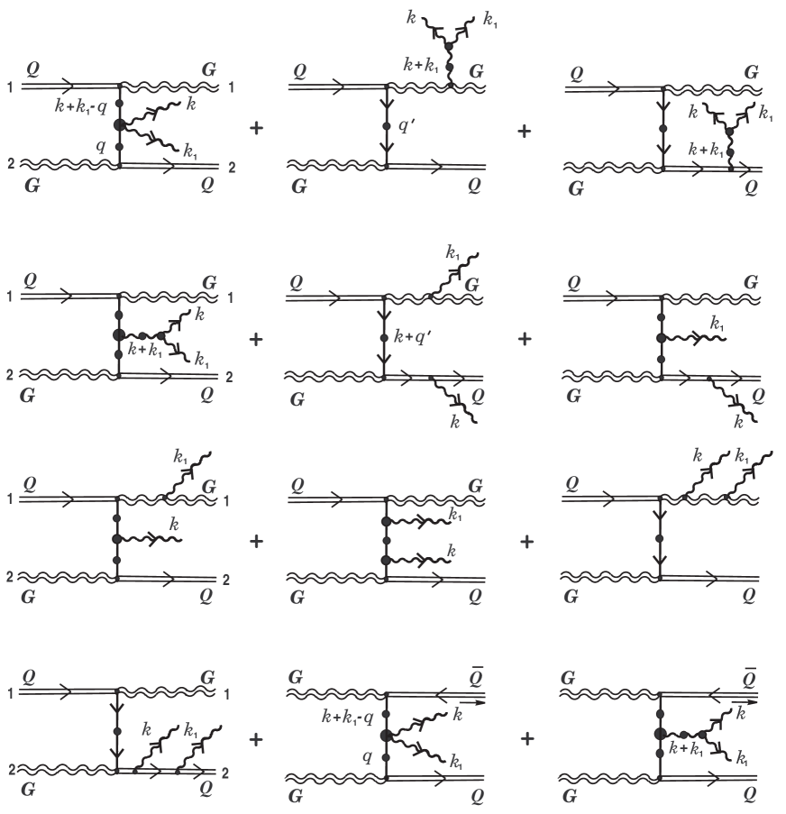
Figure 16: Some of bremsstrahlung processes of two soft gluons such that statistics of both hard particles changes. There exist also the ‘annihilation’ channel $Q\bar{Q}\rightarrow GG$gg and the channel of creation of hard quark-antiquark pair $GG\rightarrow Q\bar{Q}$gg. The last two diagrams here give examples of the latter bremsstrahlung process.

current (10.3), (10.4) this bremsstrahlung process of two soft gluons, as opposite to similar process generated by effective current (10.1), proceeds under simultaneous change of statistics of both hard particles. By way of illustration we have chosen quark and gluon as initial hard particles 1 and 2 in Fig. 16, respectively.

Further, by immediate substitution of (10.7) into (10.5) we verify that the coefficient function obtained satisfies the reality condition of the effective current. The requirement of the symmetry with respect to permutation of external soft lines leads to additional restriction on the system, namely, condition (10.6) will be fulfilled if the following equality is hold:

$$\,{}^{\ast}\Gamma^{(G)\mu}(k;q_{1},q_{2})=\,^{\ast}\Gamma^{(Q)\mu}(k;q_{1},q_{2}).$$

This equality is correct in the case when the linear Landau damping for on-shell soft excitations is absence. The only problem here arises with some quark propagators, which is similar to that with gluon propagators (see the last footnote).

We now turn our attention to the discussion of somewhat more complicated and while more interesting process: bremsstrahlung of both soft gluon and soft quark. This type of bremsstrahlung process is of particular interest in the sense that it is independently generated by either effective current or effective source. Obviously the coefficient functions in the definitions of these effective quantities are extremely to be consistent among themselves (although it is possible they do not coincide in a literal sense) since they describe the same physical process. This gives us good test to check self-consistency of all computing procedure presented in this and our previous papers.

At first we consider the effective current $\tilde{j}^{(2)a}_{\mu}$ generating the bremsstrahlung process in question. The general structure of this current is

$$\tilde{j}^{(2)a}_{\mu}[\theta_{01},\theta_{01}^{\dagger},\theta_{02},\theta_{02}^{\dagger},Q_{01},Q_{02},\psi^{(0)},\bar{\psi}^{(0)}](k)$$ (10.8)

$$=\int\!\bar{K}_{\mu,\,\alpha}^{a,\,i}({\bf v}_{1},{\bf v}_{2};\chi_{1},\chi_{2};{\bf x}_{01},{\bf x}_{02};\theta_{01}^{\dagger},\theta_{02}^{\dagger};Q_{01},Q_{02}|\,k,-q)\psi^{(0)i}_{\alpha}(q)dq,$$

$$+\,\int\!\bar{\psi}^{(0)i}_{\alpha}(-q)K_{\mu,\,\alpha}^{a,\,i}({\bf v}_{1},{\bf v}_{2};\chi_{1},\chi_{2};{\bf x}_{01},{\bf x}_{02};\theta_{01},\theta_{02};Q_{01},Q_{02}|\,k,q)dq,$$

where to leading order in the coupling constant we have

$$K_{\mu,\,\alpha}^{a,\,i}({\bf v}_{1},{\bf v}_{2};\ldots;\theta_{01},\theta_{02};Q_{01},Q_{02}|\,k,q)$$ (10.9)

$$\cong K_{\mu,\,\alpha}^{ab,\,ij}({\bf v}_{1},{\bf v}_{2};\,\ldots|\,k,q)\,\theta_{01}^{j}Q_{02}^{b}\,+\,K_{\mu,\,\alpha}^{ab,\,ij}({\bf v}_{2},{\bf v}_{1};\,\ldots|\,k,q)\,\theta_{02}^{j}Q_{01}^{b}$$

and similar expression holds good for the conjugate function $\bar{K}_{\mu,\,\alpha}^{a,\,i}$. The effective current (10.8) is presented in the form which automatically ensures its reality. To define the first coefficient function in (10.9) it needs to be considered the functional derivative of the overall current $j_{\mu}^{a}[A,\psi,\bar{\psi},\theta_{01},Q_{01},\,\ldots\,](k)$ with respect to $Q_{02},\,\theta_{01}$ and $\bar{\psi}^{(0)}$. Omitting the details of calculations, we result at once in the final expression for the desired coefficient function

$$-\left.\frac{\delta^{3}\!j^{a}_{\mu}(k)}{\delta\bar{\psi}^{(0)i}_{\alpha}(-q)\delta\theta_{01}^{j}\delta Q_{02}^{b}}\,\right|_{\,0}=K^{ab,\,ij}_{\mu,\,\alpha}({\bf v}_{1},{\bf v}_{2},;\ldots|\,k,q)$$ (10.10)

$$=\frac{\,g^{4}}{(2\pi)^{6}}\int\biggl{\{}\left[\,\delta{\Gamma}^{(G)ab,\,ij}_{\mu\nu}(k,-k-q+q^{\prime};q,-q^{\prime})\,^{\ast}\!S(q^{\prime})\chi_{1}\right]_{\alpha}\!\!\,^{\ast}{\cal D}^{\nu\nu^{\prime}}\!(k+q-q^{\prime})v_{2\nu^{\prime}}$$

$$\hskip 1.42271pt-\,(t^{b}t^{a})^{ij}\left[\,\bar{K}^{(Q)}(\bar{\chi}_{2},\chi_{2}|-k+q^{\prime},-q)\,^{\ast}\!S(k-q^{\prime})\,K_{\mu}^{(G)}({\bf v}_{1},\chi_{1}|\,k,-k+q^{\prime})\right]_{\alpha}$$

$$+\,(t^{a}t^{b})^{ij}\left[\,{}^{\ast}{\Gamma}_{\mu}^{(G)}(k;q,-k-q)\,^{\ast}\!S(k+q)\,{\cal K}({\bf v}_{2},{\bf v}_{1};\chi_{2},\chi_{1}|\,k+q,,-q^{\prime})\right]_{\alpha}\hskip 15.6491pt$$

$$+\,[t^{a},t^{b}]^{ij}\,K_{\mu\nu}({\bf v}_{2},{\bf v}_{2}|\,k,q-q^{\prime})\,^{\ast}{\cal D}^{\nu\nu^{\prime}}(-q+q^{\prime})K_{\alpha,\,\nu^{\prime}}^{(G)}({\bf v}_{1},\chi_{1}|\,-q+q^{\prime},q)\hskip 11.38092pt$$

$$+\,v_{1\mu}\chi_{1\alpha}\Biggl{\{}\frac{(t^{b}t^{a})^{ij}}{(v_{1}\cdot q)(v_{1}\cdot k)}\,-\,\frac{(t^{a}t^{b})^{ij}}{(v_{1}\cdot q)(v_{1}\cdot(k+q-q^{\,\prime}))}\Biggr{\}}\left(v_{1\nu}\!\,^{\ast}{\cal D}^{\nu\nu^{\prime}}\!(k+q-q^{\prime})v_{2\nu^{\prime}}\right)$$

$$-\,\sigma\,\{t^{a},t^{b}\}^{ij}\,\frac{v_{2\mu}\chi_{2\alpha}}{(v_{2}\cdot q)(v_{2}\cdot(k+q))}\,\left[\,\bar{\chi}_{2}\,^{\ast}\!S(q^{\prime})\chi_{1}\right]\biggr{\}}$$

$$\times\,{\rm e}^{-i{\bf q}^{\prime}\cdot\,{\bf x}_{01}}{\rm e}^{-i({\bf k}+{\bf q}-{\bf q}^{\prime})\cdot\,{\bf x}_{02}}\,\delta(v_{1}\cdot q^{\prime})\delta(v_{2}\cdot(k+q-q^{\prime}))\,dq^{\prime}.$$

The diagrammatic interpretation of the different terms in function (10.10) is presented in Fig. 17. By virtue of the structure of effective current (10.8), (10.9) one of hard particles does not change its statistics in the scattering process (for coefficient function (10.10) this is particle 2). As initial hard partons 1 and 2 in Fig. 17 we have chosen quark and gluon, respectively.

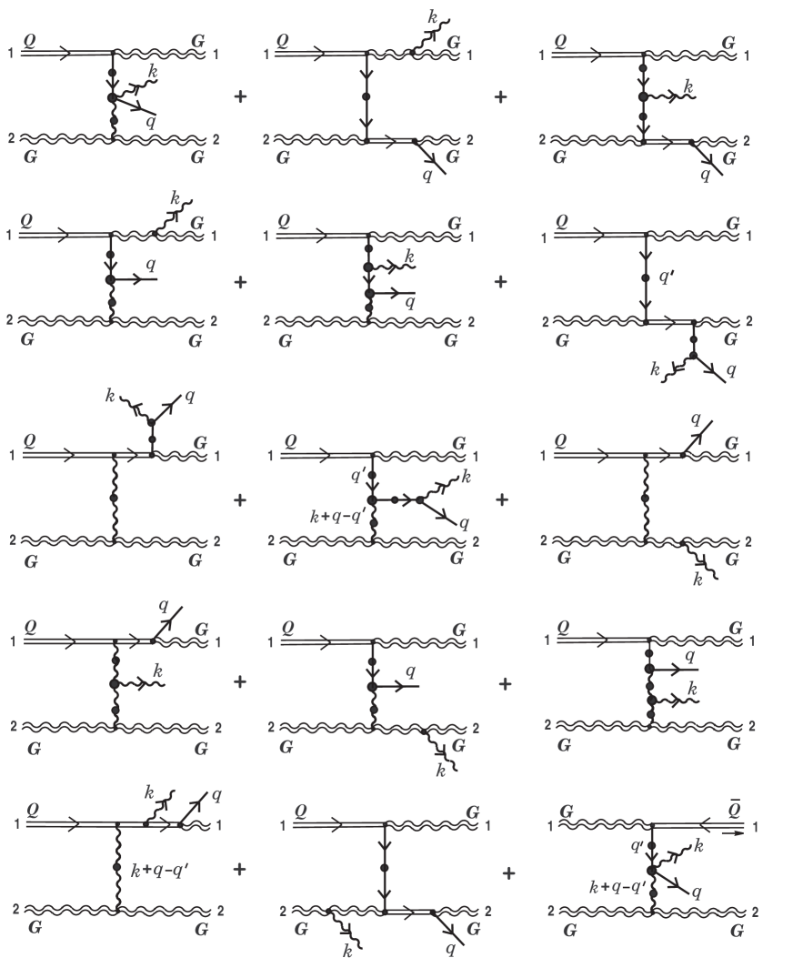
Figure 17: Bremsstrahlung of soft gluon and soft quark such that statistics of a hard parton 1 is changed. The last graph is an example of the process when both initial hard particles are gluons.

Now we consider the effective source $\tilde{\eta}_{\alpha}^{(2)i}(q)$ generating the same bremsstrahlung process. Its general structure is defined by the following expression:

$$\tilde{\eta}^{(2)a}_{\alpha}[\theta_{01},\theta_{02},Q_{01},Q_{02},A^{(0)}](k)$$

$$=\int\!K_{\alpha,\,\mu}^{i,\,a}({\bf v}_{1},{\bf v}_{2};\chi_{1},\chi_{2};{\bf x}_{01},{\bf x}_{02};\theta_{01},\theta_{02};Q_{01},Q_{02}|\,q,-k)A^{(0)a\mu}(k)dk,$$

where to leading order in $g$ we have for the coefficient function

$$K_{\alpha,\,\mu}^{i,\,a}({\bf v}_{1},{\bf v}_{2};\ldots;\theta_{01},\theta_{02};Q_{01},Q_{02}|\,q,-k)$$ (10.11)

$$\cong K_{\alpha,\,\mu}^{ij,\,ab}({\bf v}_{1},{\bf v}_{2};\,\ldots|\,q,-k)\,\theta_{01}^{j}Q_{02}^{b}\,+\,K_{\alpha,\,\mu}^{ij,\,ab}({\bf v}_{2},{\bf v}_{1};\,\ldots|\,q,-k)\,\theta_{02}^{j}Q_{01}^{b}.$$

The identical structure of expansions (10.9) and (10.11) suggests necessity of exact coincidence of the coefficient functions in the right-hand sides. However, generally this is not the case. In Appendix C we give for comparison the explicit form of the first coefficient function on the right-hand side of Eq. (10.11).

First we compare the last terms in braces in (10.10) and (C.1). For this purpose we rewrite the last term in (C.1) in the form

$$-\,\frac{1}{2}\,\alpha\,\{t^{a},t^{b}\}^{ij}\frac{v_{2\mu}\chi_{2\alpha}}{(v_{2}\cdot q)(v_{2}\cdot(q-k))}\,\left[\,\bar{\chi}_{2}\,^{\ast}\!S(q^{\prime})\chi_{1}\right]$$ (10.12)

$$\hskip 73.97733pt-\,\frac{1}{2}\,\alpha\,[t^{a},t^{b}\,]^{ij}\,\frac{v_{2\mu}\chi_{2\alpha}}{(v_{2}\cdot k)}\Biggl{(}\frac{1}{(v_{2}\cdot q)}+\frac{1}{(v_{2}\cdot(q-k))}\Biggr{)}\,\left[\,\bar{\chi}_{2}\,^{\ast}\!S(q^{\prime})\chi_{1}\right].$$

Comparing this expression with the last term in (10.10), we see that the expressions with the anticommutator $\{t^{a},t^{b}\}^{ij}$ exactly coincide with each other if in (C.1) we replace $k$ by $-k$, and for the constants $\sigma$ and $\alpha$ use the usual relation

$$\sigma=\frac{1}{2}\,\alpha.$$

The existence of the second term in (10.12) with the commutator $[t^{a},t^{b}]^{ij}$ suggests that additional current (II.5.21) which defines the last ‘eikonal’ term in (10.10), does not exhaust all additional currents to the same order in the coupling $g$ as (II.5.21).

Furthermore, next to the last terms in braces in (10.10) and (C.1) also exactly coincide under the substitution $k\rightarrow-k$ in (C.1). In the remaining terms there is no such a coincidence. This is connected mainly with the fact that in these terms there are the vertex functions which are time ordered in different way [4]. For coincidence of these terms it is necessary to perform the replacement of the type

$$\,{}^{\ast}{\Gamma}_{\mu}^{(Q)}(k;q_{1},q_{2})\rightleftharpoons\,^{\ast}{\Gamma}_{\mu}^{(G)}(k;q_{1},q_{2})$$ (10.13)

and etc. Besides, here the requirement of evenness of some propagators arises again (more precisely, for propagators like that $\,{}^{\ast}S(k-q^{\prime})$ and $\,{}^{\ast}{\cal D}(q-q^{\prime})$). If we do require an exact coincidence of the coefficient functions, i.e.

$$K^{ab,\,ij}_{\mu,\,\alpha}({\bf v}_{1},{\bf v}_{2},;\ldots|\,k,q)\equiv K^{ij,\,ab}_{\alpha,\,\mu}({\bf v}_{1},{\bf v}_{2},;\ldots|\,q,k),$$

then this imposes a number of restrictions on the system under consideration, the simplest one of which is just the above-mentioned requirement of absence of the Landau damping.

11 Bremsstrahlung of soft quark-antiquark pair and two soft (anti)quarks

In this section we will discuss bremsstrahlung process of two soft fermion excitations at collision of two hard color-charged partons. By way of the first example of such a radiation process we consider bremsstrahlung of soft quark-antiquark pair. Here, there exist two different in structure effective sources $\tilde{\eta}_{\alpha}^{(2)i}(q)$ generating the given process of bremsstrahlung. The first of them has the following structure:

$$\tilde{\eta}^{(2)i}_{\alpha}[Q_{01},Q_{02},\psi^{(0)}](q)=\int\!K_{\alpha\beta}^{ij}({\bf v}_{1},{\bf v}_{2};\chi_{1},\chi_{2};{\bf x}_{01},{\bf x}_{02};Q_{01},Q_{02}|\,q,-q_{1})\psi^{(0)j}_{\beta}(q_{1})dq_{1},$$

where for the integrand at leading order in the coupling $g$ we have

$$K_{\alpha\beta}^{ij}({\bf v}_{1},{\bf v}_{2};\,\ldots\,;Q_{01},Q_{02}|\,q,-q_{1})\cong K_{\alpha\beta}^{ij,\,ab}({\bf v}_{1},{\bf v}_{2};\ldots|\,q,-q_{1})Q_{01}^{a}Q_{02}^{b}.$$

The above expression, in particular, points to the fact that the statistics of initial hard particles 1 and 2 is not changed in this process of interaction. The coefficient function in the right-hand side is defined by variation of the total sources $\eta_{\alpha}^{i}[A,\psi,\bar{\psi},\theta_{01},Q_{01},\,\ldots\,](q)$ with respect to color charges $Q_{01},\,Q_{02}$ and free soft-fermion field $\psi^{(0)}$. The standard calculations result in the following expression for the required function

$$\left.\frac{\delta^{3}\eta^{i}_{\alpha}(k)}{\delta Q_{01}^{a}\delta Q_{02}^{b}\,\delta\psi^{(0)j}_{\beta}(q_{1})}\,\right|_{\,0}=K^{ij,\,ab}_{\alpha\beta}({\bf v}_{1},{\bf v}_{2},;\ldots|\,q,-q_{1})$$ (11.1)

$$=\frac{\,g^{4}}{(2\pi)^{6}}\int\biggl{\{}\delta{\Gamma}^{(Q)ba,\,ij}_{\mu\nu,\,\alpha\beta}(q-q_{1}-q^{\prime},q^{\prime};q_{1},-q)\!\,^{\ast}{\cal D}^{\mu\mu^{\prime}}\!(q-q_{1}-q^{\prime})v_{2\mu^{\prime}}\!\,^{\ast}{\cal D}^{\nu\nu^{\prime}}\!(q^{\prime})v_{1\nu^{\prime}}$$

$$-\,(t^{b}t^{a})^{ij}\left[K^{(Q)}(\chi_{2},\bar{\chi}_{2}|\,q,-q_{1}-q^{\prime})\,^{\ast}\!S(q_{1}+q^{\prime})\,K^{(Q)}(\chi_{1},\bar{\chi}_{1}|\,q_{1}+q^{\prime},-q_{1})\right]_{\alpha\beta}$$

$$-\,(t^{a}t^{b})^{ij}\left[K^{(Q)}(\chi_{1},\bar{\chi}_{1}|\,q,-q+q^{\prime})\,^{\ast}\!S(q-q^{\prime})\,K^{(Q)}(\chi_{2},\bar{\chi}_{2}|\,q-q^{\prime},-q_{1})\right]_{\alpha\beta}\hskip 14.22636pt$$

$$\hskip 2.84544pt-\,[t^{a},t^{b}]^{ij}\,\,{}^{\ast}{\Gamma}^{(Q)\mu}_{\alpha\beta}(q-q_{1},q_{1},-q)\!\,^{\ast}{\cal D}_{\mu\mu^{\prime}}(q-q_{1}){\cal K}^{\mu^{\prime}}({\bf v}_{1},{\bf v}_{2}|\,q-q_{1},q-q_{1}-q^{\prime})$$

$$+\,\alpha\,\chi_{2\alpha}\bar{\chi}_{2\beta}\Biggl{\{}\frac{(t^{b}t^{a})^{ij}}{(v_{2}\cdot q)(v_{2}\cdot q^{\prime})}\,-\,\frac{(t^{a}t^{b})^{ij}}{(v_{2}\cdot q_{1})(v_{2}\cdot q^{\,\prime})}\Biggr{\}}\left(v_{2\mu}\!\,^{\ast}{\cal D}^{\mu\nu}\!(q^{\prime})v_{1\nu}\right)\hskip 11.38092pt$$

$$\hskip 14.22636pt+\,\alpha\,\chi_{1\alpha}\bar{\chi}_{1\beta}\Biggl{\{}\frac{(t^{a}t^{b})^{ij}}{(v_{1}\cdot q)(v_{1}\cdot(q-q_{1}-q^{\prime}))}\,-\,\frac{(t^{b}t^{a})^{ij}}{(v_{1}\cdot q_{1})(v_{1}\cdot(q-q_{1}-q^{\,\prime}))}\Biggr{\}}$$

$$\times\left(v_{1\mu}\!\,^{\ast}{\cal D}^{\mu\nu}\!(q-q_{1}-q^{\prime})v_{2\nu}\right)\biggr{\}}$$

$$\times\,{\rm e}^{-i{\bf q}^{\prime}\cdot\,{\bf x}_{01}}{\rm e}^{-i({\bf q}-{\bf q}_{1}-{\bf q}^{\prime})\cdot\,{\bf x}_{02}}\,\delta(v_{1}\cdot q^{\prime})\delta(v_{2}\cdot(q-q_{1}-q^{\prime}))\,dq^{\prime}.$$

It is not difficult to see that this expression can be presented as

$$K_{\alpha\beta}^{ij,\,ab}({\bf v}_{1},{\bf v}_{2};\ldots|\,q,-q_{1})=(t^{a}t^{b})^{ij}K_{\alpha\beta}({\bf v}_{1},{\bf v}_{2};\ldots|\,q,-q_{1})+(t^{b}t^{a})^{ij}K_{\alpha\beta}({\bf v}_{2},{\bf v}_{1};\ldots|\,q,-q_{1}),$$

i.e., the coefficient function is symmetric with respect to permutation of external hard legs: $a\rightleftharpoons b,\,{\bf v}_{1}\rightleftharpoons{\bf v}_{2},\ldots,$ as it should be. The diagrammatic interpretation of different terms on the right-hand side of (11.1) is presented in Fig. 18. As initial hard parton 1 a quark has been chosen. In the last graph, as an example, it is depicted the process, where an initial hard parton 1 is a gluon.

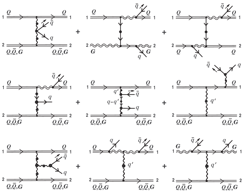
Figure 18: Process of bremsstrahlung of soft quark-antiquark pair at which the statistics of two colliding hard partons is not changed.

Furthermore, the second effective source generating the same bremsstrahlung process, is defined as follows:

$$\tilde{\eta}^{(2)i}_{\alpha}[\theta_{01},\theta_{02},\theta_{01}^{\dagger},\theta_{02}^{\dagger},\psi^{(0)}](q)$$ (11.2)

$$=\int\!K_{\alpha\beta}^{ij}({\bf v}_{1},{\bf v}_{2};\chi_{1},\chi_{2};{\bf x}_{01},{\bf x}_{02};\theta_{01},\theta_{02},\theta_{01}^{\dagger},\theta_{02}^{\dagger}|\,q,-q_{1})\psi^{(0)j}_{\beta}(q_{1})dq_{1},$$

where at leading order in the coupling constant we can set

$$K_{\alpha\beta}^{ij}({\bf v}_{1},{\bf v}_{2};\,\ldots\,;\theta_{01},\theta_{02},\theta_{01}^{\dagger},\theta_{02}^{\dagger}|\,q,-q_{1})$$

$$\cong K_{\alpha\beta}^{ij,\,kl}({\bf v}_{1},{\bf v}_{2};\,\ldots|\,q,-q_{1})\,\theta_{01}^{\dagger k}\theta_{02}^{l}\,+\,K_{\alpha\beta}^{ij,\,kl}({\bf v}_{2},{\bf v}_{1};\,\ldots|\,q,-q_{1})\,\theta_{02}^{\dagger k}\theta_{01}^{l}.$$

The right-hand side of the preceding expression is automatically symmetric with respect to permutation of external hard lines. In Appendix D the explicit form of the $K_{\alpha\beta}^{ij,\,kl}({\bf v}_{1},{\bf v}_{2};\ldots|\,q,-q_{1})$ coefficient function is given and also diagrammatic interpretation of the different terms is depicted. Here, we only mention of this function having the following structure:

$$K_{\alpha\beta}^{ij,\,kl}({\bf v}_{1},{\bf v}_{2};\,\ldots|\,q,-q_{1})$$ (11.3)

$$=(t^{a})^{ij}(t^{a})^{kl}K_{\alpha\beta}^{(1)}({\bf v}_{1},{\bf v}_{2};\,\ldots|\,q,-q_{1})+(t^{a})^{il}(t^{a})^{kj}K_{\alpha\beta}^{(2)}({\bf v}_{1},{\bf v}_{2};\,\ldots|\,q,-q_{1}),$$

where the partial coefficient functions $K_{\alpha\beta}^{(1)}$ and $K_{\alpha\beta}^{(2)}$ are not related to each other by somehow symmetry relations. Notice also that this bremsstrahlung process as distinct from previous one, occurs under simultaneous change of statistics of two colliding hard particles.

Finally, we turn to discussion of bremsstrahlung process of two soft quarks (or antiquarks) in a collision of two hard partons. We consider this radiative process in more detail. At this point, for the first time, one non-trivial destinctive feature of the theory under consideration clearly manifests itself, which turns out to be unnoticed in previous sections.

The effective source generating bremsstrahlung process we are interesting in has the following general form:

$$\tilde{\eta}^{(2)i}_{\alpha}[\theta_{01},\theta_{02},\bar{\psi}^{(0)}](q)=\!\int\!\bar{\psi}^{(0)j}_{\beta}(-q_{1})\tilde{K}_{\beta\alpha}^{ji}({\bf v}_{1},{\bf v}_{2};\chi_{1},\chi_{2};{\bf x}_{01},{\bf x}_{02};\theta_{01},\theta_{02}|\,q,q_{1})dq_{1},$$ (11.4)

where the $\tilde{K}_{\beta\alpha}^{ji}$ function in the integrand to leading order is approximated by

$$\tilde{K}_{\beta\alpha}^{ji}({\bf v}_{1},{\bf v}_{2};\,\ldots\,;\theta_{01},\theta_{02}|\,q,q_{1})\cong\tilde{K}_{\beta\alpha}^{ji,\,kl}({\bf v}_{1},{\bf v}_{2};\,\ldots|\,q,q_{1})\,\theta_{01}^{k}\theta_{02}^{l}.$$

Let us require that the effective source be symmetric with respect to permutation of external hard lines:

$$k\rightleftharpoons l,\quad{\bf v}_{1}\rightleftharpoons{\bf v}_{2},\quad\chi_{1}\rightleftharpoons\chi_{2},\;\ldots\,.$$

By virtue of anticommutativity of Grassmann color charges, the requirement results in the following condition imposed on the $\tilde{K}_{\beta\alpha}^{ij,\,kl}$ coefficient function

$$\tilde{K}_{\beta\alpha}^{ji,\,kl}({\bf v}_{1},{\bf v}_{2};\,\ldots|\,q,q_{1})=-\,\tilde{K}_{\beta\alpha}^{ji,\,lk}({\bf v}_{2},{\bf v}_{1};\,\ldots|\,q,q_{1}).$$ (11.5)

This condition in particular defines the color structure of the function under investigation

$$\tilde{K}_{\beta\alpha}^{ji,\,kl}({\bf v}_{1},{\bf v}_{2};\,\ldots|\,q,q_{1})$$ (11.6)

$$=(t^{a})^{jk}(t^{a})^{il}\tilde{K}_{\beta\alpha}({\bf v}_{1},{\bf v}_{2};\,\ldots|\,q,q_{1})-(t^{a})^{jl}(t^{a})^{ik}\tilde{K}_{\beta\alpha}({\bf v}_{2},{\bf v}_{1};\,\ldots|\,q,q_{1}).$$

Further, it would appear reasonable that the function be antisymmetric with respect to permutation of external soft fermion lines, i.e. in the case of the replacement

$$i\rightleftharpoons j,\quad\alpha\rightleftharpoons\beta,\quad q\rightleftharpoons q_{1}$$ (11.7)

the condition

$$\tilde{K}_{\beta\alpha}^{ji,\,kl}({\bf v}_{1},{\bf v}_{2};\,\ldots|\,q,q_{1})=-\,\tilde{K}_{\alpha\beta}^{ij,\,kl}({\bf v}_{1},{\bf v}_{2};\,\ldots|\,q_{1},q)$$ (11.8)

has to be held. This in turn results in a further restriction on the partial coefficient function $\tilde{K}_{\beta\alpha}$ in equation (11.6)

$$\tilde{K}_{\beta\alpha}({\bf v}_{1},{\bf v}_{2};\,\ldots|\,q,q_{1})=\tilde{K}_{\alpha\beta}({\bf v}_{2},{\bf v}_{1};\,\ldots|\,q_{1},q).$$

An explicit form of the coefficient function (11.6) is obtained from the following derivation:

$$\hskip 5.69046pt\left.\frac{\delta^{3}\eta_{\alpha}^{i}(q)}{\delta\theta_{01}^{k}\delta\theta_{02}^{j}\,\delta\bar{\psi}^{(0)j}_{\beta}(-q_{1})}\right|_{\,0}=-\,\tilde{K}^{ji,\,kl}_{\beta\alpha}({\bf v}_{1},{\bf v}_{2};\,\ldots|\,q,q_{1})$$ (11.9)

$$=\!\int\left\{\,\frac{\delta^{3}\Bigl{(}\eta_{\Xi\alpha}^{(2)i}(q)+\eta^{(2)i}_{\Omega\alpha}(q)\Bigr{)}}{\delta\psi^{j_{1}^{\prime}}_{\beta_{1}^{\prime}}(q_{1}^{\,\prime})\delta\theta_{02}^{l}\delta\bar{\psi}^{j_{2}^{\prime}}_{\beta_{2}^{\prime}}(-q_{2}^{\,\prime})}\,\Biggl{(}\frac{\psi^{j_{1}^{\prime}}_{\beta_{1}^{\prime}}(q_{1}^{\,\prime})}{\delta\theta_{01}^{k}}\Biggr{)}\Biggl{(}\frac{\bar{\psi}^{j_{2}^{\prime}}_{\beta_{2}^{\prime}}(-q_{2}^{\,\prime})}{\delta\bar{\psi}^{(0)j}_{\beta}(-q_{1})}\Biggr{)}dq_{1}^{\,\prime}dq_{2}^{\,\prime}\right.$$

$$\hskip 19.91684pt-\,\frac{\delta^{3}\Bigl{(}\eta_{\Xi\alpha}^{(2)i}(q)+\eta^{(2)i}_{\Omega\alpha}(q)\Bigr{)}}{\delta\psi^{j_{1}^{\prime}}_{\beta_{1}^{\prime}}(q_{1}^{\,\prime})\delta\theta_{01}^{k}\delta\bar{\psi}^{j_{2}^{\prime}}_{\beta_{2}^{\prime}}(-q_{2}^{\,\prime})}\,\Biggl{(}\frac{\psi^{j_{1}^{\prime}}_{\beta_{1}^{\prime}}(q_{1}^{\,\prime})}{\delta\theta_{02}^{l}}\Biggr{)}\Biggl{(}\frac{\bar{\psi}^{j_{2}^{\prime}}_{\beta_{2}^{\prime}}(-q_{2}^{\,\prime})}{\delta\bar{\psi}^{(0)j}_{\beta}(-q_{1})}\Biggr{)}dq_{1}^{\,\prime}dq_{2}^{\,\prime}$$

$$\hskip 21.33955pt+\,\frac{\delta^{2}\eta_{\alpha}^{(1,1)i}(A,\psi)(q)}{\delta A^{a_{1}^{\prime}\mu_{1}^{\prime}}(k_{1}^{\,\prime})\delta\psi^{j_{1}^{\prime}}_{\beta_{1}^{\prime}}(q_{1}^{\,\prime})}\,\Biggl{(}\frac{\delta\psi^{j_{1}^{\prime}}_{\beta_{1}^{\prime}}(q_{1}^{\,\prime})}{\delta\theta_{02}^{l}}\Biggr{)}\,\frac{\delta^{2}\!A^{a_{1}^{\prime}\mu_{1}^{\prime}}(k_{1}^{\,\prime})}{\delta\theta_{01}^{k}\,\delta\bar{\psi}^{(0)j}_{\beta}(-q_{1})}\,\,dk_{1}^{\,\prime}dq_{1}^{\,\prime}$$

$$\hskip 21.33955pt-\,\frac{\delta^{2}\eta_{\alpha}^{(1,1)i}(A,\psi)(q)}{\delta A^{a_{1}^{\prime}\mu_{1}^{\prime}}(k_{1}^{\,\prime})\delta\psi^{j_{1}^{\prime}}_{\beta_{1}^{\prime}}(q_{1}^{\,\prime})}\,\Biggl{(}\frac{\delta\psi^{j_{1}^{\prime}}_{\beta_{1}^{\prime}}(q_{1}^{\,\prime})}{\delta\theta_{01}^{k}}\Biggr{)}\,\frac{\delta^{2}\!A^{a_{1}^{\prime}\mu_{1}^{\prime}}(k_{1}^{\,\prime})}{\delta\theta_{02}^{l}\,\delta\bar{\psi}^{(0)j}_{\beta}(-q_{1})}\,\,dk_{1}^{\,\prime}dq_{1}^{\,\prime}$$

$$\left.+\,\frac{\delta^{2}\eta_{\theta_{2}\alpha}^{(1)i}(q)}{\delta\theta_{02}^{l}\,\delta A^{a_{1}^{\prime}\mu_{1}^{\prime}}(k_{1}^{\,\prime})}\,\frac{\delta^{2}\!A^{a_{1}^{\prime}\mu_{1}^{\prime}}(k_{1}^{\,\prime})}{\delta\theta_{01}^{k}\,\delta\bar{\psi}^{(0)j}_{\beta}(-q_{1})}\;dk_{1}^{\,\prime}\,-\,\frac{\delta^{2}\eta_{\theta_{1}\alpha}^{(1)i}(q)}{\delta\theta_{01}^{k}\,\delta A^{a_{1}^{\prime}\mu_{1}^{\prime}}(k_{1}^{\,\prime})}\,\frac{\delta^{2}\!A^{a_{1}^{\prime}\mu_{1}^{\prime}}(k_{1}^{\,\prime})}{\delta\theta_{02}^{l}\,\delta\bar{\psi}^{(0)j}_{\beta}(-q_{1})}\;dk_{1}^{\,\prime}\right\}.$$

With the help of an explicit form of the sources on the right-hand side of (11.9) we obtain the following expression for the desired coefficient function:

$$\tilde{K}^{ji,\,kl}_{\beta\alpha}({\bf v}_{1},{\bf v}_{2};\,\ldots|\,q,q_{1})$$ (11.10)

$$=\frac{g^{4}}{(2\pi)^{6}}\,\int\Biggl{\{}\!\Bigl{[}\,\beta\,(t^{a})^{ik}(t^{a})^{jl}+\,\beta_{1}(t^{a})^{il}(t^{a})^{jk\,}\Bigr{]}\frac{\chi_{1\alpha}\chi_{1\beta}}{(v_{1}\cdot q^{\prime})(v_{1}\cdot q_{1})}\,\left[\,\bar{\chi}_{1}\,^{\ast}\!S(q^{\prime})\chi_{2}\right]\hskip 99.58464pt$$

$$\hskip 51.21504pt-\,\Bigl{[}\,\beta\,(t^{a})^{il}(t^{a})^{jk}+\,\beta_{1}(t^{a})^{ik}(t^{a})^{jl\,}\Bigr{]}\frac{\chi_{2\alpha}\chi_{2\beta}}{(v_{2}\cdot(q+q_{1}-q^{\prime}))(v_{2}\cdot q_{1})}\,\left[\,\bar{\chi}_{2}\,^{\ast}\!S(q+q_{1}-q^{\prime})\chi_{1}\right]$$

$$\hskip 14.22636pt+\,(t^{a})^{il}(t^{a})^{jk}K^{(Q)\mu}_{\alpha}({\bf v}_{2},\chi_{2}|\,q-q^{\prime},-q)\,^{\ast}{\cal D}_{\mu\nu}(q-q^{\prime})K^{(G)\nu}_{\beta}({\bf v}_{1},\chi_{1}|\,q-q^{\prime},q_{1})$$

$$\hskip 34.14322pt-\,(t^{a})^{ik}(t^{a})^{jl}K^{(Q)\mu}_{\alpha}({\bf v}_{1},\chi_{1}|\,q^{\prime}-q_{1},-q)\,^{\ast}{\cal D}_{\mu\nu}(q^{\prime}-q_{1})K^{(G)\nu}_{\beta}({\bf v}_{2},\chi_{2}|\,q^{\prime}-q_{1},q_{1})\!\Biggr{\}}$$

$$\times\,{\rm e}^{-i({\bf q}+{\bf q}_{1}-{\bf q}^{\prime})\cdot\,{\bf x}_{01}}{\rm e}^{-i{\bf q}^{\prime}\cdot\,{\bf x}_{02}}\,\delta(v_{1}\cdot(q+q_{1}-q^{\prime}))\delta(v_{2}\cdot q^{\prime})\,dq^{\prime}.$$

The diagrammatic interpretation of various terms in (11.10) is given in Fig. 19. By virtue of the structure of the effective source, in this scattering process the statistics of both hard particles changes.

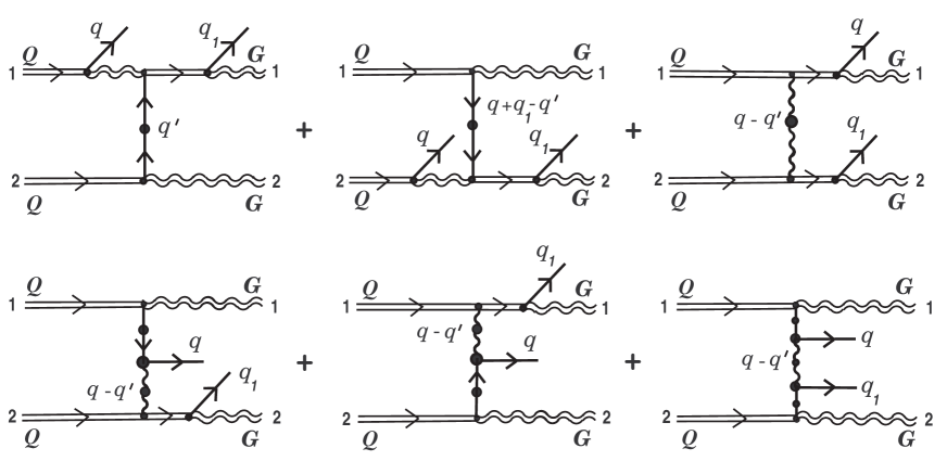
Figure 19: Bremsstrahlung of two soft quarks. As initial hard partons here hard quarks have been chosen.

By using an explicit expression (11.10) it is not difficult to verify that the condition of antisymmetry with respect to permutation hard external legs (11.5) is hold. The situation with condition (11.8) is more complicated. At first we consider two last terms in braces in Eq. (11.10). When one rearranges external soft fermionic lines by equation (11.7), the third term in the integrand in (11.10) transforms to the last with the opposite sign and vice versa. In so doing simultaneously we must replace the vertex functions according to (10.13). Besides, here a requirement of evenness for gluon propagators of the ${}^{\ast}{\cal D}_{\mu\nu}(q_{1}-q^{\prime})$ type arises.

Further, consider the first two ‘eikonal’ terms in (11.10). It is not difficult to see that these terms in the case of permutation (11.7) do not transform neither into itself (with opposite sign) nor into each other. This suggests that we do not take into account further contribution or other which would antisymmetrize the coefficient function in question. All additional sources introduced in Paper II do not already provide a necessary condition of antisymmetry with respect to soft quark external lines. Additional eikonal terms in (11.10), restoring fermion statistics for these lines, must be also generated by the first two derivations in the right-hand side of (11.9) as well as the eikonal terms in hand.

We see the resolution of the problem along the following line. Let us consider the Grassmann color source induced by a hard test particle (it was introduced in Paper II, Eq. (II.3.8))

$$\eta_{\theta\alpha}^{i}(x)=g\theta^{i}(t)\chi_{\alpha}{\delta}^{(3)}({\bf x}-{\bf v}t).$$ (11.11)

Here,

$$\theta^{i}(t)=U^{ij}(t,t_{0})\theta_{0}^{j},$$

where

$$U(t,t_{0})={\rm T}\exp\Biggl{\{}-ig\!\int\limits_{t_{0}}^{t}(v\cdot A^{a}(\tau,{\bf v}\tau))\,t^{a}d\tau\!\Biggr{\}}$$ (11.12)

is the known evolution operator in the fundamental representation. In Paper II (Appendix A) we have attempted to construct the Lagrangian such that in the case of differentiation with respect to soft fields $A_{\mu},\,\psi$ and $\bar{\psi}$ it would correctly reproduce the Yang-Mills and Dirac equations with all additional currents and sources on the right-hand sides. Such Lagrangian have been defined. However, if we vary the Lagrangian with respect to hard component of the system, i.e. with respect to Grassmann color charges $\theta^{i}(t)$ and $\theta^{\dagger i}(t)$, then in the evolution equations for these charges (II.5.8) new terms of higher order in soft fields $\psi,\,\bar{\psi}$ appear. The particular consequence of this fact is that instead of the evolution operator (11.12) it is necessary to introduce the extended evolution operator ${\cal U}(t,t_{0})$ (II.A.6) which takes into account the effect of rotation of color charge in inner color space induced by both soft gauge and soft quark stochastic fields. We also pointed out that the influence of soft quark field on the rotation should be taken into account in the scattering processes of the third order in powers of free fermion fields $\psi_{0}$ and $\bar{\psi}_{0}$, and the initial values of Grassmann charges $\theta_{0}^{i}$ and $\theta_{0}^{\dagger i}$. The situation we are facing above in dealing with (11.10) is just concerns this case.

In a first approximation the extended evolution operator may be taken as follows:

$${\cal U}(t,t_{0})\simeq 1-ig\!\int\limits_{t_{0}}^{t}(v^{\mu}A_{\mu}^{a}(\tau,{\bf v}\tau))t^{a}d\tau$$

$$-\,ig\,\hat{\alpha}\!\int\limits_{t_{0}}^{t}\Biggl{[}\,(\bar{\psi}_{\alpha}^{k}(\tau,{\bf v}\tau){\chi}_{\alpha})\,t^{a}\Biggl{(}-ig\!\int\limits_{t_{0}}^{\tau}(\bar{\chi}_{\beta}\psi_{\beta}(\tau^{\,\prime},{\bf v}\tau^{\,\prime\,}))d\tau^{\,\prime}\Biggr{)}\Biggr{]}d\tau\,t^{a}$$

$$-\,ig\,\hat{\alpha}^{\ast}\!\int\limits_{t_{0}}^{t}\Biggl{[}\,\Biggl{(}ig\!\int\limits_{t_{0}}^{\tau}(\bar{\psi}_{\beta}(\tau^{\,\prime},{\bf v}\tau^{\,\prime\,})\chi_{\beta})d\tau^{\,\prime}\Biggr{)}t^{a}(\bar{\chi}_{\alpha}\psi_{\alpha}(\tau,{\bf v}\tau))\Biggr{]}d\tau\,t^{a}\hskip 4.26773pt$$

$$\hskip 11.38092pt-\,ig\,\hat{\beta}\!\int\limits_{t_{0}}^{t}\Biggl{[}\,\Biggl{(}-ig\!\int\limits_{t_{0}}^{\tau}\!t^{a}(\bar{\chi}_{\beta}\psi_{\beta}(\tau^{\,\prime},{\bf v}\tau^{\,\prime\,}))d\tau^{\,\prime}\Biggr{)}\!\otimes(\bar{\psi}_{\alpha}(\tau,{\bf v}\tau){\chi}_{\alpha})t^{a}\Biggr{]}d\tau$$

$$\hskip 9.95863pt-\,ig\,\hat{\beta}^{\ast}\!\int\limits_{t_{0}}^{t}\Biggl{[}\,t^{a}(\bar{\chi}_{\alpha}\psi_{\alpha}(\tau,{\bf v}\tau))\otimes\!\Biggl{(}ig\!\int\limits_{t_{0}}^{\tau}(\bar{\psi}_{\beta}(\tau^{\,\prime},{\bf v}\tau^{\,\prime\,})\chi_{\beta})t^{a}d\tau^{\,\prime}\Biggr{)}\Biggr{]}d\tau,$$

where $\hat{\alpha},\,\hat{\beta}$ are some (complex) parameters and $\otimes$ is a symbol of the direct production. Our interest here is only with the last four terms. Let us define now an evolution of the Grassmann color charge in the following way:

$$\theta^{i}(t)={\cal U}^{ij}(t,t_{0})\theta_{0}^{j}$$

with the evolution operator written out just above. Further, substitute this color charge into the initial source (11.11). Performing the Fourier transform of this source, we obtain a new derivation (additional to (II.5.20))

$$\left.\frac{\delta^{3}\eta_{\alpha}^{i}[A,\psi,\theta_{0}](q)}{\delta\psi^{i_{1}}_{\alpha_{1}}(q_{1})\delta\bar{\psi}^{i_{2}}_{\alpha_{2}}(-q_{2})\delta\theta_{0}^{j}}\,\right|_{\,0}$$ (11.13)

$$=\frac{\,g^{3}}{(2\pi)^{3}}\,\Bigl{[}\,\hat{\alpha}(t^{a})^{ij}(t^{a})^{i_{2}i_{1}}-\hat{\beta}(t^{a})^{ii_{1}}(t^{a})^{i_{2}j\,}\Bigr{]}\frac{\chi_{\alpha}\bar{\chi}_{\alpha_{1}}\chi_{\alpha_{2}}}{(v\cdot q_{1})(v\cdot q)}\,\,\delta(v\cdot(q+q_{2}-q_{1}))$$

$$\hskip 14.22636pt+\,\frac{\,g^{3}}{(2\pi)^{3}}\,\Bigl{[}\,\hat{\alpha}^{\ast}(t^{a})^{ij}(t^{a})^{i_{2}i_{1}}-\hat{\beta}^{\ast}(t^{a})^{ii_{1}}(t^{a})^{i_{2}j\,}\Bigr{]}\frac{\chi_{\alpha}\bar{\chi}_{\alpha_{1}}\chi_{\alpha_{2}}}{(v\cdot q_{2})(v\cdot q)}\,\,\delta(v\cdot(q+q_{2}-q_{1})).$$

Let us return to the coefficient function of interest. The first two derivations in (11.9) lead to appearing new eikonal terms in the integrand in (11.10) if derivation (11.13) is accounted for, namely

$$[\,\hat{\alpha}\,(t^{a})^{ik}(t^{a})^{jl}-\,\hat{\beta}(t^{a})^{il}(t^{a})^{jk}]\frac{\chi_{1\alpha}{\chi}_{1\beta}}{(v_{1}\cdot q^{\prime})(v_{1}\cdot q)}\,\left[\,\bar{\chi}_{1}\,^{\ast}\!S(q^{\prime})\chi_{2}\right]\hskip 48.36958pt$$ (11.14)

$$\hskip 38.41139pt-\,[\,\hat{\alpha}\,(t^{a})^{il}(t^{a})^{jk}-\,\hat{\beta}(t^{a})^{ik}(t^{a})^{jl}]\frac{\chi_{2\alpha}{\chi}_{2\beta}}{(v_{2}\cdot(q+q_{1}-q^{\prime}))(v_{2}\cdot q)}\,\left[\,\bar{\chi}_{2}\,^{\ast}\!S(q+q_{1}-q^{\prime})\chi_{1}\right]$$

$$+\,[\,\hat{\alpha}^{\ast}\,(t^{a})^{ik}(t^{a})^{jl}-\,\hat{\beta}^{\ast}(t^{a})^{il}(t^{a})^{jk}]\frac{\chi_{1\alpha}{\chi}_{1\beta}}{(v_{1}\cdot q_{1})(v_{1}\cdot q)}\,\left[\,\bar{\chi}_{1}\,^{\ast}\!S(q^{\prime})\chi_{2}\right]\hskip 48.36958pt$$

$$\hskip 28.45274pt-\,[\,\hat{\alpha}^{\ast}\,(t^{a})^{il}(t^{a})^{jk}-\,\hat{\beta}^{\ast}(t^{a})^{ik}(t^{a})^{jl}]\frac{\chi_{2\alpha}{\chi}_{2\beta}}{(v_{2}\cdot q_{1})(v_{2}\cdot q)}\,\left[\,\bar{\chi}_{2}\,^{\ast}\!S(q+q_{1}-q^{\prime})\chi_{1}\right].\hskip 28.45274pt$$

Now we demand that the sum of two first terms in (11.14) along with the first two terms in (11.10) should satisfy condition (11.8). This will take place if we set

$$\hat{\alpha}\equiv-\,\beta_{1}\qquad\hat{\beta}\equiv\beta.$$

We demand further that the remaining two terms in (11.14) should turn into itself with the opposite sign in case of permutation (11.7). This imposes one more additional condition on parameters $\hat{\alpha}$ and $\hat{\beta}$:

$$\hat{\alpha}=\hat{\beta}.$$

It is not difficult to verify that new contributions (11.14) do not violate the condition of antisymmetry with respect to permutation of external hard lines, Eq. (11.5). Thus at the cost of introducing the extended evolution operator we can restore antisymmetry of coefficient function (11.10) with respect to external soft fermion lines.

In closing it is necessary to look back and indicate new eikonal contributions which should be added to the effective sources calculated early. There exist two such sources. The first of them is the effective source of bremsstrahlung of soft quark-antiquark pair when statistics of both hard partons (Eq. (11.2)) changes. Additional eikonal terms generated by derivation (11.13), which should be added to coefficient function (D.1) are given at the end of Appendix D, equation (D.2).

The effective source (6.8) generating bremsstrahlung of one soft quark in the case of collision of three hard partons is the second effective source, where also new contributions appear. This scattering process change statistics of every hard particle as well. The following new terms:

$$\frac{g^{5}}{(2\pi)^{9}}\int\biggl{\{}\!\Bigl{[}\,\hat{\alpha}\,(t^{a})^{ik}(t^{a})^{jl}-\,\hat{\beta}(t^{a})^{il}(t^{a})^{jk\,}\Bigr{]}\frac{\chi_{2\alpha}}{(v_{2}\cdot k^{\prime})(v_{2}\cdot q^{\prime})}\,\left[\,\bar{\chi}_{1}\,^{\ast}\!S(k^{\prime}-q^{\prime})\chi_{2}\right]\left[\,\bar{\chi}_{2}\,^{\ast}\!S(q^{\prime})\chi_{3}\right]$$

$$-\,\Bigl{[}\,\hat{\alpha}^{\ast}\,(t^{a})^{ik}(t^{a})^{jl}-\,\hat{\beta}^{\ast}(t^{a})^{il}(t^{a})^{jk\,}\Bigr{]}\frac{\chi_{2\alpha}}{(v_{2}\cdot k^{\prime})(v_{2}\cdot(k^{\prime}-q^{\prime}))}\,\left[\,\bar{\chi}_{1}\,^{\ast}\!S(k^{\prime}-q^{\prime})\chi_{2}\right]\left[\,\bar{\chi}_{2}\,^{\ast}\!S(q^{\prime})\chi_{3}\right]$$

$$\hskip 227.62204pt-\,(2\rightleftharpoons 3,\,k\rightleftharpoons l)\biggr{\}}$$

$$\times\,{\rm e}^{-i({\bf k}^{\prime}-\,{\bf q}^{\prime})\cdot\,{\bf x}_{01}}{\rm e}^{-i({\bf q}-{\bf k}^{\prime})\cdot\,{\bf x}_{02}}{\rm e}^{-i{\bf q}^{\prime}\cdot\,{\bf x}_{03}}\,\delta(v_{1}\cdot(k^{\prime}-q^{\prime}))\delta(v_{2}\cdot(q-k^{\prime}))\delta(v_{3}\cdot q^{\prime})\,dk^{\prime}dq^{\prime}$$

should be added to the coefficient function (6.10).

12 Conclusion

In this final part of our work we have presented the scheme of successive construction of the effective theory for radiative processes in the hot quark-gluon plasma including on equal terms soft excitations both Fermi-Dirac and Bose-Einstein statistics. By various examples we have made an attempt to show efficiency of the approach suggested in this paper for calculation of probabilities of bremsstrahlung processes up to the third order in powers of free soft fermionic and bosonic fields and the initial values of color charges of hard particles. Unfortunately, the use of the proposed dynamical equations (II.5.8) and (II.5.11) for the color charges $\theta^{i}(t),\,\theta^{\dagger i}(t)$ and $Q^{a}(t)$, and also additional currents and sources introduced in Paper II, turns out to be insufficient for correct construction of some effective sources (section 11) already in the third order. For the appropriate description of the processes under consideration a necessity of adding in the dynamical equations the terms of higher order in powers of interacting soft fermion fields, arises. It is evident that in research of more complicated radiative processes we are faced with a necessity of defining an explicit form of higher-order additional currents and sources in the coupling constant than in [2], and also a necessity of further modification of equations for the color charges. Here it is desirable to have an algorithm making it possible automatically to define all relevant quantities to any order in powers of soft fields and color charges.

Further recall that the evolution equations (II.5.8) and (II.5.11), and also an explicit form of additional currents and sources (II.5.14), (II.5.18), and so on, have been obtained mainly from considerations of heuristic character. The gauge covariance of the equations, currents and sources is the major requirement in their construction. But here, another point arises: the gauge covariance is necessary of course, but is it sufficient in this case? For successive construction of an effective theory of radiative processes in the QGP and rigorous justification of the results obtained, we come up against the problem of derivation of the evolution equations for classical color charges proceed from the first principles within the framework of quantum field theory. Obtaining Wong’s equation for the usual color charge in [6] and equations for the Grassmann color charges in an external gauge field in [25] provides an example of such derivation from the first principles. These equations can be justified as a semiclassical approximation to the world-line formulation of the one-loop effective action in QCD. However, attempt of direct including external fermion field into the developed approaches unexpectedly encounters severe problems of technical and fundamental nature. Here we can only points to the fact that in principle, two different in the conceptual plan approaches to a rigorous derivation of the required evolution equations, are possible.

The first of them, more straightforward approach, is connected with immediate semiclassical approximation of the quantum Dirac equation in arbitrary external fields. At present there exists powerful mathematically well-founded method of deriving classical equations of motion directly from the equations of motion for the quantum expectation values of a certain set of observables. This method is known as the complex WKB-Maslov one or the complex germ theory [17]. Maslov’s approach have been successfully applied to the equations of both non-relativistic and relativistic quantum mechanics. The further development of this method has resulted in discovery of so-called semiclassical trajectory-coherent states (TCS) [18, 19, 20] generalizing the well-known coherent states to the case of an arbitrary external field. These states have the advantage that they make it possible to calculate the $\hbar\rightarrow 0$ limit for the expectation values of quantum observables that have no classical analogs, for example, the particle spin (see [21]). For the case of an arbitrary electromagnetic field (the group $U(1)$), complete orthonormalized set of semiclassical TCSs has been constructed with any degree of accuracy in the Planck constant for the Dirac equation with anomalous Pauli interaction in [21, 20]. In the paper [22] similar states were constructed for the Dirac operator in an arbitrary chromoelectromagnetic field with the gauge group $SU(2)$. These states were used to derive classical equations of motion and in particular, the Wong equation from the equations of relativistic quantum mechanics for a non-Abelian charge. The next step here, is the extension of the scheme of semiclassical approximation of the Dirac equation suggested in works [21, 20], to a case when in the system under consideration along with an external vector bosonic field there exists also an external fermionic field.

The second to some extent more indirect approach appeals to the world-line formulation of quantum field theory. In considerable amount of papers it was shown that the one-loop effective actions for scalar models, QED and QCD could be expressed in terms of a quantum mechanical path integral over a point particle Lagrangian. In case of the QCD coupling the world-line path integral representation was obtained not only for the effective action for quark loop, but for gluon one in an external non-Abelian field as well [23, 24]. One of the important steps here was made by D’Hoker and Gagné [25]. They have presented the internal color degrees of freedom in terms of world-line fermions expressed by independent dynamical Grassmann variables $\theta^{\dagger i}(t)$ and $\theta^{i}(t)$. These are precisely that color charges we have used throughout Paper II and the present work, and first introduced in the papers [16] from other less rigorous reasons. By this means for rigorous proof of the evolution equations (II.5.8) and (II.5.11), it is necessary to consider more general problem: the world-line path integral representation of the one-loop QCD action (or equivalent of functional superdeterminant [26]) at simultaneously presence of external gauge and fermionic fields. To the best of our knowledge the given problem has not considered in the literature.

Unfortunately, as already was mentioned above, attempt of direct extension of the developed approaches to the solution of this problem causes great difficulties both conceptual and technical character. The presence of a fermionic background field leads to qualitatively new phenomenon: a single background fermion can change the particle in the loop from a Dirac spinor into a vector boson and vice versa. Therefore our task is to build a theory which consistently describes a particle that can be either quark or gluon. From the mathematical point of view this means that it is necessary to obtain an explicit form of the fermion vertex operator which is inserted into the world closed line of the hard particle and defines the radiation (or absorption) process of an external quark simulated by an external fermionic background. The construction of this vertex operator is necessary ingredient of rigorous derivation of the evolution equations for color charges.

One way of looking at the solution of the problem in hand (and in particular of computation of the desired vertex operator) is in terms of the string theory. At one time in a number of works [27] the problem of the propagation of (super)string in background fields was considered. As shown in [28], background space-time fermions may be incorporated into the string action on equal terms with the other external fields if to use the covariant string vertex operator [29]. As far as we know, this is the only rigorous inclusion of interaction with an external fermion field which is well understood. Here it can be applied one of the heuristic arguments that the required fermion vertex for the first-quantized field theory is related in a certain way with the fermion vertex operator of superstring theory. The efficiency of the string-based methods in concrete applications to the problems of calculation of the pure gluon one-loop QCD amplitudes was demonstrated in the early 1990s by Bern and Kosower [30] and then by the others. Now the purpose is to extend the well-developed approach to incorporate external quarks.

Thus, in the light of the above-mentioned, one can outline another way of derivation of the evolution equations from the first principles. The first step is attempt to define in the context of superstring-inspired approach [30] an explicit form of one-loop QCD amplitude including both external bosons and external fermions. Then as a following step will be an attempt to guess an explicit form of the effective action in the world-line formulation which on expanding in powers of the background fields would reproduce the mixed quark-gluon one-loop amplitudes obtained at the first stage. And the final step would be the world-line representation for the color degree of freedom of hard particle running in the mixed loop in the spirit of D’Hoker and Gagné [25]. Here one can propose that by virtue of the mixed character of statistics of the particle in the loop we obtain a point particle Lagrangian containing simultaneously on equal terms both usual color charge $Q^{a}(t)$ and Grassmann color charges $\theta^{\dagger i}(t)$, $\theta^{i}(t)$. These charges can be combined into a single color supercharge (see footnote 9). By varying the action obtained by this strategy with respect to the supercharge, we obtain the desired evolution equations. All this is the subject of our further research.

Appendix A

The medium modified quark propagator $\,{}^{\ast}\!S(q)$ we use throughout this work, has the following form:

$$\,{}^{\ast}\!S(q)=h_{+}(\hat{\mathbf{q}})\,^{\ast}\!\triangle_{+}(q)+h_{-}(\hat{\mathbf{q}})\,^{\ast}\!\triangle_{-}(q),$$

where the matrix functions $h_{\pm}(\hat{\bf q})=(\gamma^{0}\mp\hat{{\bf q}}\cdot\vec{\gamma}\,)/2$ with $\hat{{\bf q}}\equiv{\bf q}/|{\bf q}|$ are the spinor projectors onto eigenstates of helicity and

$$\,{}^{\ast}\!\triangle_{\pm}(q)=-\,\frac{1}{q^{0}\mp[\,|{\bf q}|+\delta\Sigma_{\pm}(q)]}$$

are the ‘scalar’ quark propagators, where in turn

$$\delta\Sigma_{\pm}(q)=\frac{\omega_{0}^{2}}{|{\mathbf{q}}|}\biggl{[}\,1-\biggl{(}1\mp\frac{|{\mathbf{q}}|}{q^{0}}\biggr{)}F\biggl{(}\frac{q^{0}}{|{\mathbf{q}}|}\biggr{)}\biggr{]}$$

with

$$F(z)=\frac{z}{2}\biggl{[}\,\ln\bigg{|}\frac{1+z}{1-z}\bigg{|}-i\pi\theta(1-|z|)\biggr{]}$$

are the scalar quark self-energies for normal $(+)$ and plasmino $(-)$ modes.

Further, we give an explicit form of the scalar vertex functions between a quark pair and a gluon (the HTL-effects are neglected here) deeply used in sections 4 and 5. Omitting the color matrix $t^{a}$ and the factor $ig$, the bare vertex

$$\Gamma^{\mu}=\Gamma^{\mu}(k;l,-q)\equiv\gamma^{\mu}$$

can be identically rewritten for spatial part $\mu=i$ by either of two ways [32, 2]:

$$\Gamma^{i}=-\,h_{-}(\hat{\bf l}){\it\Gamma}_{+}^{\,i}-h_{+}(\hat{\bf l}){\it\Gamma}_{-}^{\,i}+2h_{-}(\hat{\bf q})\,{\bf l}^{2}|{\bf q}|{\it\Gamma}_{\perp}^{\,i}+({\bf n}\cdot\vec{\gamma}){\it\Gamma}_{\!1\perp}^{\,i},$$

or

$$\Gamma^{i}=-\,h_{-}(\hat{\bf l})\acute{{\it\Gamma}}_{+}^{\,i}-h_{+}(\hat{\bf l})\acute{{\it\Gamma}}_{-}^{\,i}-2h_{+}(\hat{\bf q})\,{\bf l}^{2}|{\bf q}|{\it\Gamma}_{\perp}^{\,i}+({\bf n}\cdot\vec{\gamma}){\it\Gamma}_{\!1\perp}^{\,i}.$$

Here, the scalar vertex functions are

$${\it\Gamma}_{\pm}^{\,i}\equiv\mp|{\bf l}|{\it\Gamma}_{\parallel}^{\,i}+\frac{{\bf n}^{2}}{|{\bf q}|}\,\frac{1}{1\mp\hat{\bf q}\cdot\hat{\bf l}}\,{\it\Gamma}_{\perp}^{\,i},\quad\acute{{\it\Gamma}}_{\pm}^{\,i}\equiv\mp|{\bf l}|{\it\Gamma}_{\parallel}^{\,i}-\frac{{\bf n}^{2}}{|{\bf q}|}\,\frac{1}{1\pm\hat{\bf q}\cdot\hat{\bf l}}\,{\it\Gamma}_{\perp}^{\,i},\quad{\it\Gamma}_{\!1\perp}^{\,i}\equiv\frac{{\bf n}^{i}}{{\bf n}^{2}},$$

where ${\it\Gamma}_{\parallel}^{\,i}=l^{i}/{\bf l}^{2},\,{\it\Gamma}_{\perp}^{\,i}=({\bf n}\times{\bf l})^{i}/{\bf n}^{2}{\bf l}^{2},\;{\bf l}={\bf q}-{\bf k}$, and ${\bf n}=({\bf q}\times{\bf k})$.

Appendix B

In this Appendix we go into technical details of calculation of the trace (5.2). For convenience of further references we write out here once more the form of initial expression rearranging only the matrix $h_{+}(\hat{\bf q})$ on cycle:

$${\rm Sp}\!\left[\Bigl{(}h_{+}(\hat{\bf q}){\cal M}h_{+}(\hat{\bf q}_{1})\Bigr{)}\Bigl{(}\gamma^{0}{\cal M}^{\dagger}\gamma^{0}\Bigr{)}\right],$$

where

$${\cal M}=\frac{\alpha}{4E_{1}}\,\frac{(v_{1}\cdot\gamma)}{(v_{1}\cdot q_{1})}\,-\,^{\ast}\Gamma^{(Q)\mu}(q-q_{1};q_{1},-q)\!\,^{\ast}{\cal D}_{\mu\nu}(q-q_{1})v_{1}^{\nu}.$$

The resummed gluon propagator in (B.2) is conveniently defined here in the temporal gauge

$$\,{}^{\ast}{\cal D}_{\mu\nu}(l)=-P_{\mu\nu}(l)\,^{\ast}\!\Delta^{t}(l)-\tilde{Q}_{\mu\nu}(l)\,^{\ast}\!\Delta^{l}(l)+\xi_{0}\frac{l^{2}}{(l\cdot u)^{2}}\frac{l_{\mu}l_{\nu}}{l^{2}},\quad l\equiv q-q_{1},$$

where $\xi_{0}$ is a gauge-fixing parameter; $P_{\mu\nu}(l)$ and $\tilde{Q}_{\mu\nu}(l)$ are the transverse and longitudinal projectors that in the rest frame of the heat bath, $u_{\mu}=(1,0,0,0)$, are equal to

$$P_{\mu\nu}(l)=-\left(\begin{array}[]{cc}0&0\\ 0&1-\displaystyle\frac{{\bf l}\otimes{\bf l}}{{\bf l}^{2}}\end{array}\right),\quad\tilde{Q}_{\mu\nu}(l)=\left(\begin{array}[]{cc}0&0\\ 0&-\,\displaystyle\frac{l^{2}}{l_{0}^{2}}\,\displaystyle\frac{{\bf l}\otimes{\bf l}}{{\bf l}^{2}}\end{array}\right).$$

By using the effective Ward identity for the HTL-resummed vertex $\,{}^{\ast}\Gamma^{(Q)\mu}$, it is easy to verify that the term with $\xi_{0}$ vanishes on mass-shell of soft fermion excitations.

First we consider the last term in amplitude (B.2). The vertex $\,{}^{\ast}\Gamma^{(Q)\mu}$ according to (A.5) can be presented in the form of two different decompositions. For the first decomposition by virtue of nilpotency property $(h_{+}(\hat{\bf q}))^{2}=(h_{+}(\hat{\bf q}_{1}))^{2}=0$ we have

$$\left(h_{+}(\hat{\bf q})\,^{\ast}\Gamma^{(Q)i}(l;q_{1},-q)h_{+}(\hat{\bf q}_{1})\right)$$

$$=\,-\,[\,h_{+}(\hat{\bf q})h_{-}(\hat{\bf q}_{1})h_{+}(\hat{\bf q}_{1})]\,^{\ast}\!\acute{{\it\Gamma}}_{+}^{\,i}(l;q_{1},-q)\,+\,[\,h_{+}(\hat{\bf q})({\bf n}\cdot\vec{\gamma})h_{+}(\hat{\bf q}_{1})]\,^{\ast}\!{\it\Gamma}_{\!1\perp}^{\,i}(l;q_{1},-q),$$

and respectively, for the second decomposition we can write

$$\left(h_{+}(\hat{\bf q})\,^{\ast}\Gamma^{(Q)i}(l;q_{1},-q)h_{+}(\hat{\bf q}_{1})\right)\equiv\left(h_{+}(\hat{\bf q})\,^{\ast}\Gamma^{(Q)i}(-l;q,-q_{1})h_{+}(\hat{\bf q}_{1})\right)$$

$$\hskip 14.22636pt=\,-\,[\,h_{+}(\hat{\bf q})h_{-}(\hat{\bf q})h_{+}(\hat{\bf q}_{1})]\,^{\ast}\!\acute{{\it\Gamma}}_{+}^{\,i}(-l;q,-q_{1})\,-\,[\,h_{+}(\hat{\bf q})({\bf n}\cdot\vec{\gamma})h_{+}(\hat{\bf q}_{1})]\,^{\ast}\!{\it\Gamma}_{\!1\perp}^{\,i}(-l;q,-q_{1}).$$

Let us put together these two expressions and divide the sum obtained by two. Taking into account an explicit form of projectors (B.3) and the identity

$$\delta^{ij}-\,\frac{l^{i}l^{j}}{{\bf l}^{2}}=\frac{n^{i}n^{j}}{{\bf n}^{2}}\,+\,\frac{({\bf n}\times{\bf l})^{i}({\bf n}\times{\bf l})^{j}}{{\bf n}^{2}\,{\bf l}^{2}}\,,\quad{\bf n}\equiv({\bf q}_{1}\times{\bf q}),$$

we obtain instead of the last term in (B.2) surrounded by the matrices $h_{+}(\hat{\bf q})$ and $h_{+}(\hat{\bf q}_{1})$ the following expression:

$$\frac{1}{2}\,[\,h_{+}(\hat{\bf q})h_{-}(\hat{\bf q}_{1})h_{+}(\hat{\bf q}_{1})]\Biggl{\{}\!\Biggl{(}\frac{l^{2}}{l_{0}^{2}\,{\bf l}^{2}}\Biggr{)}\Bigl{(}\,^{\ast}\!\acute{{\it\Gamma}}_{+}^{\,i}(l;q_{1},-q)l^{i}\,\Bigr{)}\,^{\ast}\!\Delta^{l}(l)\,({\bf v}_{1}\cdot{\bf l})\hskip 85.35826pt$$

$$\hskip 136.5733pt+\,\frac{1}{{\bf n}^{2}\,{\bf l}^{2}}\,\Bigl{(}\,^{\ast}\!\acute{{\it\Gamma}}_{+}^{\,i}(l;q_{1},-q)({\bf n}\times{\bf l})^{i}\,\Bigr{)}\,^{\ast}\!\Delta^{t}(l)\,({\bf v}_{1}\cdot({\bf n}\times{\bf l}))\Biggr{\}}$$

$$+\,\frac{1}{2}\,[\,h_{+}(\hat{\bf q})h_{-}(\hat{\bf q})h_{+}(\hat{\bf q}_{1})]\Biggl{\{}\!\Biggl{(}\frac{l^{2}}{l_{0}^{2}\,{\bf l}^{2}}\Biggr{)}\Bigl{(}\,^{\ast}\!\acute{{\it\Gamma}}_{+}^{\,i}(-l;q,-q_{1})l^{i}\,\Bigr{)}\,^{\ast}\!\Delta^{l}(l)\,({\bf v}_{1}\cdot{\bf l})\hskip 62.59596pt$$

$$\hskip 147.95424pt+\,\frac{1}{{\bf n}^{2}\,{\bf l}^{2}}\,\Bigl{(}\,^{\ast}\!\acute{{\it\Gamma}}_{+}^{\,i}(-l;q,-q_{1})({\bf n}\times{\bf l})^{i}\,\Bigr{)}\,^{\ast}\!\Delta^{t}(l)\,({\bf v}_{1}\cdot({\bf n}\times{\bf l}))\!\Biggr{\}}$$

$$-\,\frac{1}{2}\,[\,h_{+}(\hat{\bf q})({\bf n}\cdot\vec{\gamma})h_{+}(\hat{\bf q}_{1})]\Bigl{\{}\!\,^{\ast}\!{\it\Gamma}_{\!1\perp}^{\,i}(l;q_{1},-q)n^{i}-\,^{\ast}\!{\it\Gamma}_{\!1\perp}^{\,i}(-l;q,-q_{1})n^{i}\Bigr{\}}\,\frac{({\bf v}_{1}\cdot{\bf n})}{{\bf n}^{2}}\,\,^{\ast}\!\Delta^{t}(l).\hskip 17.07182pt$$

Now we proceed to analysis of the first term in (B.2). Let us rewrite this term in the following form beforehand having multiply from the left by $h_{+}(\hat{\bf q})$ and from the right by $h_{+}(\hat{\bf q}_{1})$

$$\frac{\alpha}{4E_{1}}\,\frac{1}{(v_{1}\cdot q_{1})}\,\Bigl{\{}[\,h_{+}(\hat{\bf q})\gamma_{0}\,h_{+}(\hat{\bf q}_{1})]\,-\,[\,h_{+}(\hat{\bf q})({\bf v}_{1}\cdot\vec{\gamma}\,)h_{+}(\hat{\bf q}_{1})]\Bigr{\}}.$$

Let us present the $\gamma_{0}$ matrix in an identical form

$$\gamma_{0}=\frac{1}{2}\,\Bigl{\{}\Bigl{(}h_{-}(\hat{\bf q}_{1})+h_{+}(\hat{\bf q}_{1})\Bigr{)}+\Bigl{(}h_{-}(\hat{\bf q})+h_{+}(\hat{\bf q})\Bigr{)}\Bigr{\}}.$$

By virtue of the above-mentioned nilpotency property the terms with $h_{+}(\hat{\bf q})$ and $h_{+}(\hat{\bf q}_{1})$ can be omitted. Next we rewrite the scalar product ${\bf v}_{1}\cdot\vec{\gamma}=v^{i}_{1}\delta^{ij}\gamma^{j}$ in the form of the expansion in terms of the transverse and longitudinal projectors with respect to the vector of momentum transfer ${\bf l}$:

$$v_{1}^{i}\,(\delta^{ij}-\hat{l}^{i}\hat{l}^{j}\,)\,\gamma^{j}\,+\,({\bf v}_{1}\cdot\hat{\bf l})(\vec{\gamma}\cdot\hat{\bf l}),\quad\hat{\bf l}\equiv{\bf l}/|{\bf l}|.$$

By using the definition of the matrices $h_{+}(\hat{\bf q})$ and $h_{+}(\hat{\bf q}_{1})$ it is not difficult to see that the product $(\vec{\gamma}\cdot\hat{\bf l})$ can be presented in the form of the expansion in terms of these matrices

$$\vec{\gamma}\cdot\hat{\bf l}\,\cong\frac{1}{|{\bf l}|}\,\Bigl{\{}|{\bf q}|\,h_{-}(\hat{\bf q})-|{\bf q}_{1}|\,h_{-}(\hat{\bf q}_{1})\Bigr{\}}.$$

The symbol $\cong$ means that the terms with the matrices $h_{+}(\hat{\bf q})$ and $h_{+}(\hat{\bf q}_{1})$ here are omitted.

Furthermore, for the term with the transverse projector in (B.7) we make use identity (B.4)

$$v^{i}_{1}\,(\delta^{ij}-\hat{l}^{i}\hat{l}^{j}\,)\,\gamma^{j}=\frac{({\bf v}_{1}\cdot{\bf n})(\vec{\gamma}\cdot{\bf n})}{{\bf n}^{2}}\,+\,\frac{({\bf v}_{1}\cdot({\bf n}\times{\bf l}))}{{\bf n}^{2}\,{\bf l}^{2}}\,(\vec{\gamma}\cdot({\bf n}\times{\bf l}))\,.$$

It is easy to verify that the last term on the right-hand side of (B.8) admits again the decomposition in terms of the spinor projectors $h_{+}(\hat{\bf q})$ and $h_{+}(\hat{\bf q}_{1})$:

$$\vec{\gamma}\cdot({\bf n}\times{\bf l})\cong h_{-}(\hat{\bf q})|{\bf q}|({\bf l}\cdot{\bf q}_{1})-h_{-}(\hat{\bf q}_{1})|{\bf q}_{1}|({\bf l}\cdot{\bf q}).$$

Taking into account all the above-mentioned, we get instead of (B.6)

$$\hskip 19.91684pt\frac{1}{4E_{1}}\,\frac{\alpha}{(v_{1}\cdot q_{1})}\,[\,h_{+}(\hat{\bf q})h_{-}(\hat{\bf q}_{1})h_{+}(\hat{\bf q}_{1})]\Biggl{\{}\Biggl{(}\frac{1}{2}\,\frac{|{\bf l}|}{l^{0}}+\frac{|{\bf q}_{1}|}{|{\bf l}|}\Biggr{)}\frac{({\bf v}_{1}\cdot{\bf l})}{|{\bf l}|}\,+\,\frac{|{\bf q}_{1}|({\bf l}\cdot{\bf q})}{{\bf n}^{2}\,{\bf l}^{2}}\,({\bf v}_{1}\cdot({\bf n}\times{\bf l}))\Biggr{\}}$$

$$+\,\frac{1}{4E_{1}}\,\frac{\alpha}{(v_{1}\cdot q_{1})}\,[\,h_{+}(\hat{\bf q})h_{-}(\hat{\bf q})h_{+}(\hat{\bf q}_{1})]\Biggl{\{}\Biggl{(}\frac{1}{2}\,\frac{|{\bf l}|}{l^{0}}-\frac{|{\bf q}|}{|{\bf l}|}\Biggr{)}\frac{({\bf v}_{1}\cdot{\bf l})}{|{\bf l}|}\,-\,\frac{|{\bf q}|({\bf l}\cdot{\bf q}_{1})}{{\bf n}^{2}\,{\bf l}^{2}}\,({\bf v}_{1}\cdot({\bf n}\times{\bf l}))\Biggr{\}}$$

$$-\,\frac{1}{4E_{1}}\,\frac{\alpha}{(v_{1}\cdot q_{1})}\,[\,h_{+}(\hat{\bf q})({\bf n}\cdot\vec{\gamma})h_{+}(\hat{\bf q}_{1})]\,\frac{({\bf v}_{1}\cdot{\bf n})}{{\bf n}^{2}}\,.\hskip 182.09746pt$$

Remarkable feature of the expressions (B.5) and (B.9) is a distinctive factorization of the spinor dependence in the function $\left(h_{+}(\hat{\bf q}){\cal M}\,h_{+}(\hat{\bf q}_{1})\right)$. Subtracting (B.5) from (B.9) and making use the definition of scalar amplitudes (5.3), finally we derive

$$\Bigl{(}h_{+}(\hat{\bf q}){\cal M}h_{+}(\hat{\bf q}_{1})\Bigr{)}$$

$$=\frac{1}{2}\,[\,h_{+}(\hat{\bf q})h_{-}(\hat{\bf q}_{1})h_{+}(\hat{\bf q}_{1})]\left\{{\cal M}_{l}({\bf p}_{1}|\,{\bf q},{\bf q}_{1})({\bf v}_{1}\cdot{\bf l})\,+\,{\cal M}_{t}({\bf p}_{1}|\,{\bf q},{\bf q}_{1})\,\frac{({\bf v}_{1}\cdot({\bf n}\times{\bf l}))}{{\bf n}^{2}\,{\bf l}^{2}}\right\}$$

$$-\,\frac{1}{2}\,[\,h_{+}(\hat{\bf q})h_{-}(\hat{\bf q})h_{+}(\hat{\bf q}_{1})]\left\{{\cal M}_{l}^{\ast}({\bf p}_{1}|\,{\bf q}_{1},{\bf q})({\bf v}_{1}\cdot{\bf l})\,-{\cal M}_{t}^{\ast}({\bf p}_{1}|\,{\bf q}_{1},{\bf q})\,\frac{({\bf v}_{1}\cdot({\bf n}\times{\bf l}))}{{\bf n}^{2}\,{\bf l}^{2}}\right\}\hskip 2.84544pt$$

$$-\,\frac{1}{2}\,[\,h_{+}(\hat{\bf q})({\bf n}\cdot\vec{\gamma})h_{+}(\hat{\bf q}_{1})]\,\Bigl{\{}{\cal M}_{\!1t}({\bf p}_{1}|\,{\bf q},{\bf q}_{1})\,+\,{\cal M}_{\!1t}^{\ast}({\bf p}_{1}|\,{\bf q}_{1},{\bf q})\Bigr{\}}\frac{({\bf v}_{1}\cdot{\bf n})}{{\bf n}^{2}}\,.\hskip 55.48277pt$$

Further, we can also present the trace (B.1) in the form

$${\rm Sp}\!\left[{\cal M}\Bigl{(}h_{+}(\hat{\bf q}_{1})(\gamma^{0}{\cal M}^{\dagger}\gamma^{0})h_{+}(\hat{\bf q})\Bigr{)}\right].$$

We have the evident relation $\Bigl{(}h_{+}(\hat{\bf q}_{1})(\gamma^{0}{\cal M}^{\dagger}\gamma^{0})h_{+}(\hat{\bf q})\Bigr{)}\!=\!\gamma^{0}\Bigl{(}h_{+}(\hat{\bf q}){\cal M}\,h_{+}(\hat{\bf q}_{1})\Bigr{)}^{\!\dagger}\!\gamma^{0}$. In this relation under the sign of Hermitian conjunction the above-defined expression (B.10) stands. By this means taking into account the equalities $(h_{+}(\hat{\bf q}))^{\dagger}\!=\!\gamma^{0}h_{+}(\hat{\bf q})\gamma^{0}$ and $(h_{+}(\hat{\bf q}_{1}))^{\dagger}=\gamma^{0}h_{+}(\hat{\bf q}_{1})\gamma^{0}$, it is not difficult to see that the calculation of initial trace (B.1) reduces to calculations of a few simple traces:

$${\rm Sp}\,[h_{-}(\hat{\bf q}_{1})h_{+}(\hat{\bf q}_{1})h_{-}(\hat{\bf q}_{1})h_{+}(\hat{\bf q})]=1+\hat{\bf q}\cdot\hat{\bf q}_{1}\,,$$

$$\hskip 17.07182pt{\rm Sp}\,[h_{+}(\hat{\bf q}_{1})({\bf n}\cdot\vec{\gamma})h_{+}(\hat{\bf q})({\bf n}\cdot\vec{\gamma})]=(1-\hat{\bf q}\cdot\hat{\bf q}_{1})\,{\bf n}^{2},$$

$${\rm Sp}\,[h_{+}(\hat{\bf q}_{1})h_{-}(\hat{\bf q}_{1})h_{+}(\hat{\bf q})({\bf n}\cdot\vec{\gamma})]=0,\hskip 45.52458pt$$

and so on, that results finally in formula (5.2).

Appendix C

Here we give an explicit expression for the $K_{\alpha,\,\mu}^{ij,\,ab}({\bf v}_{1},{\bf v}_{2};\,\ldots|\,q,-k)$ coefficient function defining the bremsstrahlung process of a soft gluon and a soft quark simultaneously

$$K_{\alpha,\,\mu}^{ij,\,ab}({\bf v}_{1},{\bf v}_{2};\chi_{1},\chi_{2};{\bf x}_{01},{\bf x}_{02}|\,q,-k)$$

$$=\frac{\,g^{4}}{(2\pi)^{6}}\int\biggl{\{}\left[\,\delta{\Gamma}^{(Q)ba,\,ij}_{\nu\mu}(q-k-q^{\prime},k;q^{\prime},-q)\,^{\ast}\!S(q^{\prime})\chi_{1}\right]_{\alpha}\!\!\,^{\ast}{\cal D}^{\nu\nu^{\prime}}\!(q-k-q^{\prime})v_{2\nu^{\prime}}$$

$$\hskip 11.38092pt-\,(t^{b}t^{a})^{ij}\left[\,K^{(Q)}(\chi_{2},\bar{\chi}_{2}|\,q,-k-q^{\prime})\,^{\ast}\!S(k+q^{\prime})\,K_{\mu}^{(Q)}({\bf v}_{1},\chi_{1}|\,k,-k-q^{\prime})\right]_{\alpha}$$

$$\hskip 35.85031pt-\,(t^{a}t^{b})^{ij}\left[\,{}^{\ast}{\Gamma}_{\mu}^{(Q)}(k;-k+q,-q)\,^{\ast}\!S(-k+q)\,{\cal K}({\bf v}_{2},{\bf v}_{1};\chi_{2},\chi_{1}|-\!k+q,,-q^{\prime})\right]_{\alpha}$$

$$\hskip 5.69046pt-\,[t^{a},t^{b}]^{ij}\,K_{\alpha,\,\nu^{\prime}}^{(Q)}({\bf v}_{1},\chi_{1}|\,q-q^{\prime},-q)\,^{\ast}{\cal D}^{\nu^{\prime}\nu}(q-q^{\prime})K_{\nu\mu}({\bf v}_{2},{\bf v}_{2}|\,q-q^{\prime},-k)$$

$$-\,v_{1\mu}\chi_{1\alpha}\Biggl{\{}\frac{(t^{b}t^{a})^{ij}}{(v_{1}\cdot q)(v_{1}\cdot k)}\,+\,\frac{(t^{a}t^{b})^{ij}}{(v_{1}\cdot q)(v_{1}\cdot(q-k-q^{\,\prime}))}\Biggr{\}}\left(v_{1\nu}\!\,^{\ast}{\cal D}^{\nu\nu^{\prime}}\!(q-k-q^{\prime})v_{2\nu^{\prime}}\right)$$

$$+\,\alpha\,v_{2\mu}\chi_{2\alpha}\Biggl{\{}\frac{(t^{b}t^{a})^{ij}}{(v_{2}\cdot q)(v_{2}\cdot k)}\,-\,\frac{(t^{a}t^{b})^{ij}}{(v_{2}\cdot q^{\prime})(v_{2}\cdot k)}\Biggr{\}}\left[\,\bar{\chi}_{2}\,^{\ast}\!S(q^{\prime})\chi_{1}\right]\biggr{\}}$$

$$\times\,{\rm e}^{-i{\bf q}^{\prime}\cdot\,{\bf x}_{01}}{\rm e}^{-i({\bf q}-{\bf k}-{\bf q}^{\prime})\cdot\,{\bf x}_{02}}\,\delta(v_{1}\cdot q^{\prime})\delta(v_{2}\cdot(q-k-q^{\prime}))\,dq^{\prime}.$$

The graphic interpretation of various terms on the right-hand side of Eq. (C.1) is the same as in Fig. 17.

Appendix D

In this Appendix we give an explicit form of the coefficient function (11.3). The function is defined through the third order derivative of the total source with respect to Grassmann charges $\theta_{01}^{\dagger k}$ and $\theta_{02}^{l}$, and a free soft-quark field $\psi^{(0)}$:

$$-\left.\frac{\delta^{3}\eta_{\alpha}^{i}(q)}{\delta\theta_{01}^{\dagger k}\delta\theta_{02}^{l}\delta\psi_{\beta}^{(0)j}(q_{1})}\,\right|_{\,0}=\,K^{ij,\,kl}_{\alpha\beta}({\bf v}_{1},{\bf v}_{2};\,\ldots|\,q,-q_{1})$$

$$=\frac{g^{4}}{(2\pi)^{6}}\int\biggl{\{}\!\Bigl{[}\,\beta\,(t^{a})^{il}(t^{a})^{kj}+\,\beta_{1}(t^{a})^{ij}(t^{a})^{kl\,}\Bigr{]}\frac{\chi_{2\alpha}\bar{\chi}_{2\beta}}{(v_{2}\cdot q_{1})(v_{2}\cdot(q-q_{1}-q^{\prime}))}\,\left[\,\bar{\chi}_{1}\,^{\ast}\!S(q-q_{1}-q^{\prime})\chi_{2}\right]$$

$$-\,(t^{a})^{ij}(t^{a})^{kl}\,{}^{\ast}\Gamma^{(Q)\mu}_{\alpha\beta}(q-q_{1};q_{1},-q)\,^{\ast}{\cal D}_{\mu\nu}(q-q_{1})[\,\bar{\chi}_{1\,}{\cal K}^{\nu}({\bf v}_{1},{\bf v}_{2}|\,q-q_{1},-q^{\prime})\chi_{2}]$$

$$-\,(t^{a})^{il}(t^{a})^{kj}\,K_{\alpha}^{(G)\mu}({\bf v}_{2},\chi_{2}|-\!q+q^{\prime},q)\,^{\ast}{\cal D}_{\mu\nu}(q-q^{\prime})\,\bar{K}_{\beta}^{(G)\nu}({\bf v}_{1},\bar{\chi}_{1}|\,q-q^{\prime},-q_{1})$$

$$\hskip 42.67912pt-\,\tilde{\beta}_{1}\,\Bigl{[}\,(t^{a})^{ij}(t^{a})^{kl}-\,(t^{a})^{il}(t^{a})^{kj\,}\Bigr{]}\,\frac{\chi_{1\alpha}\bar{\chi}_{1\beta}}{(v_{1}\cdot q_{1})(v_{1}\cdot q^{\prime})}\,\left[\,\bar{\chi}_{1}\,^{\ast}\!S(q^{\prime})\chi_{2}\right]\biggr{\}}$$

$$\times\,{\rm e}^{-i({\bf q}-{\bf q}_{1}-{\bf q}^{\prime})\cdot\,{\bf x}_{01}}{\rm e}^{-i{\bf q}^{\prime}\cdot\,{\bf x}_{02}}\,\delta(v_{1}\cdot(q-q_{1}-q^{\prime}))\delta(v_{2}\cdot q^{\prime})\,dq^{\prime}.$$

The diagrammatic interpretation of different terms on the right-hand side is presented in Fig. 20. These graphs should be added to those depicted in Fig. 18. As initial hard particles 1 and 2, by way of illustration, in Fig. 20 a quark and a gluon have been chosen, respectively.

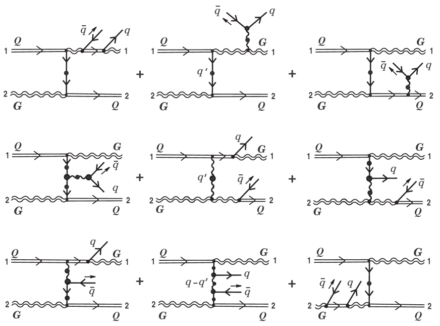
Figure 20: Bremsstrahlung of soft quark-antiquark pair such that the statistics of both hard initial partons changes.

To the above-written coefficient function (D.1) must be added two terms of the eikonal type that generated by derivative (11.13):

$$-\,\frac{g^{4}}{(2\pi)^{6}}\int\biggl{\{}\!\Bigl{[}\,\hat{\alpha}\,(t^{a})^{il}(t^{a})^{kj}-\,\hat{\beta}(t^{a})^{ij}(t^{a})^{kl\,}\Bigr{]}\frac{\chi_{2\alpha}\bar{\chi}_{2\beta}}{(v_{2}\cdot q)(v_{2}\cdot q_{1})}\,\left[\,\bar{\chi}_{1}\,^{\ast}\!S(q-q_{1}-q^{\prime})\chi_{2}\right]$$

$$\hskip 65.72578pt-\Bigl{[}\,\hat{\alpha}^{\ast}(t^{a})^{il}(t^{a})^{kj}-\,\hat{\beta}^{\ast}(t^{a})^{ij}(t^{a})^{kl\,}\Bigr{]}\frac{\chi_{2\alpha}\bar{\chi}_{2\beta}}{(v_{2}\cdot q)(v_{2}\cdot(q-q_{1}))}\,\left[\,\bar{\chi}_{1}\,^{\ast}\!S(q-q_{1}-q^{\prime})\chi_{2}\right]\biggr{\}}$$

$$\times\,{\rm e}^{-i({\bf q}-{\bf q}_{1}-{\bf q}^{\prime})\cdot\,{\bf x}_{01}}{\rm e}^{-i{\bf q}^{\prime}\cdot\,{\bf x}_{02}}\,\delta(v_{1}\cdot(q-q_{1}-q^{\prime}))\delta(v_{2}\cdot q^{\prime})\,dq^{\prime}.$$

This contribution takes into account influence of stochastic soft fermionic fields in the system on rotation of Grassmann color charges $\theta^{i}(t)$ and $\theta^{i\dagger}(t)$ of a hard particle (see section 11).

References

• [1] Yu.A. Markov, M.A. Markova, Nucl. Phys. A 770 (2006) 162.
• [2] Yu.A. Markov, M.A. Markova, Nucl. Phys. A 784 (2007) 443.
• [3] B. Vanderheyden, J.-Y. Ollitrault, Phys. Rev. D 56 (1997) 5108.
• [4] J.-P. Blaizot, E. Iancu, Nucl. Phys. B 417 (1994) 608.
• [5] L.D. McLerran, R. Venugopalan, Phys. Rev. D 49 (1994) 2233; 49 (1994) 3352; 50 (1994) 2225.
• [6] J. Jalilian-Marian, S. Jeon, R. Venugopalan, and J. Wirstam, Phys. Rev. D 62 (2000) 045020.
• [7] J. Jalilian-Marian, S. Jeon, R. Venugopalan, Phys. Rev. D 63 (2001) 036004; S. Jeon, R. Venugopalan, Phys. Rev. D 70 (2004) 105012.
• [8] K. Fukushima, Nucl. Phys. A 770 (2006) 71.
• [9] B. Bistrovic, R. Jackiw, H. Li, V.P. Nair, and S.-Y. Pi, Phys. Rev. D 67 (2003) 025013.
• [10] B.W.A. Leurs, Z. Nazario, D.I. Santiago, and J. Zaanen, Ann. Phys. (N.Y.) 323 (2008) 907.
• [11] S.R. de Groot, W.A. van Leeuwen, and Ch.G. van Weert, Relativistic Kinetic Theory, North-Holland, Amsterdam, 1980.
• [12] W. Liu, C.M. Ko, B.W. Zhang, Phys. Rev. C 75 (2007) 051901; W. Liu, R.J. Fries, Phys. Rev. C 77 (2008) 054902.
• [13] Yu.A. Markov, M.A. Markova, A.N. Vall, Ann. Phys. (N.Y.) 320 (2005) 282.
• [14] B.G. Zakharov, JETP Lett. 63 (1996) 952; 65 (1997) 615.
• [15] R. Baier, Yu.L. Dokshitzer, A.H. Mueller, and D. Schiff, Nucl. Phys. B 531 (1998) 403; M. Gyulassy, P. Levai, I. Vitev, Nucl. Phys. B 594 (2001) 371.
• [16] A. Barducii, R. Casalbuoni, L. Lusanna, Nucl. Phys. B 124 (1977) 93; A.P. Balachandran, P. Salomonson, B. Skagerstam, and J. Winnberg, Phys. Rev. D 15 (1977) 2308.
• [17] V.P. Maslov, Operator Methods, Nauka, Moscow, 1973; V.P. Maslov, The Complex WKB Method in Nonlinear Equations, Nauka, Moscow, 1977.
• [18] V.G. Bagrov, V.V. Belov, I.M. Ternov, Teor. Math. Fiz. 50 (1982) 390 (English transl. in Theor. Math. Phys. 50 (1982) 261); J. Math. Phys. 24 (1983) 2855.
• [19] V.G. Bagrov, V.V. Belov, A.Yu. Trifonov, Ann. Phys. (N.Y.) 246 (1996) 231.
• [20] V.G. Bagrov, V.V. Belov, A.Yu. Trifonov, unpublished. Available from: $\langle$quant-ph/9806017$\rangle$.
• [21] V.V. Belov, V.P. Maslov, Dokl. AN SSSR 305 (1989) 574 (English transl. in Sov. Phys. Dokl. 34 (1989) 220); Dokl. AN SSSR 311 (1990) 849 (English transl. in Sov. Phys. Dokl. 35 (1990) 330).
• [22] V.V. Belov, M.F. Kondrat’eva, Teor. Math. Fiz. 92 (1992) 41 (English transl. in Theor. Math. Phys. 92 (1992) 722).
• [23] M.J. Strassler, Nucl. Phys. B 385 (1992) 145.
• [24] M. Reuter, M.G. Schmidt, C. Schubert, Ann. Phys. (N.Y.) 259 (1997) 313.
• [25] E.D. D’Hoker, D.G. Gagné, Nucl. Phys. B 467 (1996) 272; 467 (1996) 297.
• [26] P. Elmfors, T.H. Hansson, I. Zahed, Phys. Rev. D 59 (1999) 045018.
• [27] C. Lovelace, Phys. Lett. B 135 (1984) 75; E. Fradkin, A. Tseytlin, Phys. Lett. B 158 (1985) 316; A. Sen, Phys. Rev. Lett. 55 (1985) 1846.
• [28] C.G. Callan, D. Friedan, E.J. Martinec, and M.J. Perry, Nucl. Phys. B 262 (1985) 593.
• [29] V.G. Knizhnik, Phys. Lett. B 160 (1985) 403; D. Friedan, E.J. Martinec, S. Shenker, Nucl. Phys. B 271 (1986) 93.
• [30] Z. Bern, D.A. Kosower, Nucl. Phys. B 379 (1992) 451.
• [31] Z. Bern, L. Dixon, D.A. Kosower, Nucl. Phys. B 437 (1995) 259.
• [32] Yu.A. Markov, M.A. Markova, Phys. Rev. D 64 (2001) 105009.