On the conformally coupled scalar field quantum cosmology

Abstract

We propose a new initial condition for the homogeneous and isotropic quantum cosmology, where the source of the gravitational field is a conformally coupled scalar field, and the maximally symmetric hypersurfaces have positive curvature. After solving corresponding Wheeler-DeWitt equation, we obtain exact solutions in both classical and quantum levels. We propose appropriate initial condition for the wave packets which results in a complete classical and quantum correspondence. These wave packets closely follow the classical trajectories and peak on them. We also quantify this correspondence using de-Broglie Bohm interpretation of quantum mechanics. Using this proposal, the quantum potential vanishes along the Bohmian paths and the classical and Bohmian trajectories coincide with each other. We show that the model contains singularities even at the quantum level. Therefore, the resulting wave packets closely follow the classical trajectories from big-bang to big-crunch.

1 Introduction

In recent years, the question of construction and interpretation of wave packets in quantum cosmology and its connection with classical cosmology has attracted much attention. Moreover, some attempts have done to construct a theory of quantum gravity and find its relation with classical physics. Some authors use the semiclassical approximations for the Wheeler-DeWitt (WDW) equation and consider the oscillatory or exponentially decaying solutions in the configuration space as classically allowed or forbidden regions, respectively. These regions are mainly determined by the initial conditions for the wave function of the universe. The no-boundary proposal of Hartle and Hawking [1] and the quantum creation of the universe from nothingness by Vilenkin [2] are two popular proposals for the initial conditions.

In quantum cosmology similar to the ordinary quantum mechanics, one is usually concerned with the construction of wave functions by the superposition of the energy eigenfunctions which would peak around the classical trajectories and follow them in configuration space, whenever such classical and quantum correspondence is possible [3, 4, 5]. However, contrary to the ordinary quantum mechanics, an external time parameter is absent in the theory of quantum cosmology. Therefore, the initial conditions would have to be formulated with respect to intrinsic time parameter, which could be taken as the local scale factor for the three-geometry in the case of the hyperbolic WDW equation [6].

The construction of wave packets resulting from the solutions of the WDW equation is a common feature of some investigations in quantum cosmology [7, 8, 9, 10]. To be more specific, in Refs. [10, 11] the construction of wave packets in a Friedmann-Robertson-Walker (FRW) universe with a minimally coupled self interacting scalar field is presented and appropriate initial conditions are motivated. In Ref. [12], the authors investigated $(n+1)$-dimensional quantum cosmology with varying speed of light and obtained exact solutions in both classical and quantum domains. The wave packets are constructed in such a way that they completely correspond to their unique classical counterparts. In Ref. [13], a class of spherically symmetric Stephani cosmological models with a minimally coupled scalar field is studied in both classical and quantum levels [14, 15]. The aim of these investigations has been to find wave packets whose probability distributions coincide with the classical paths obtained in classical cosmology. This means that the wave packet should be centered around the classical path and its crest should closely follow the classical trajectory.

Here, we study a minisuperspace model describing a closed FRW universe with vanishing cosmological constant and containing a conformally coupled scalar field. The issue of the conformally coupled scalar field quantum cosmology has been in vogue for more than twenty years and basic results have been found by several authors [3, 4, 16, 17, 18, 19, 20, 21, 22, 23, 24, 25, 26, 27]. In particular, Page [20] has also studied this model and after solving the resulting WDW equation he obtained the solutions for the positive, negative and zero curvatures. For the case of positive curvature, the WDW equation casts into a oscillator-ghost-oscillator differential equation with well-known solutions. Moreover, Barbosa [26] has used one or two of these solutions to construct the wave packets and found the Bohmian trajectories via de-Broglie Bohm interpretation of quantum mechanics. Therefore, in contrast to the classical scenario, he found some non-singular solutions. In fact, the Bohmian trajectories highly depend on the wave function of the system and various linear combinations of eigenfunctions lead to different Bohmian trajectories. On the other hand, since the underlying WDW equation is second-order hyperbolic functional differential equation, we are free to choose the initial wave function and the initial slope of the wave function. But classically, we have a unique solution. Therefore, we encounter with a meaningful question: Is it possible to choose the initial condition in such a way that the resulting wave packet completely corresponds to its unique classical counterpart? In the previous investigations, using appropriate initial conditions (expansion coefficients), we could construct the wave packets which completely simulate their classical counterparts [11, 12, 13]. In particular, in Ref. [13], we obtained the wave packets so that the quantum potential vanishes along the Bohmian trajectories. In fact, the behavior of the quantum solution is strictly dependent to the initial conditions imposed on the wave function. Here, at the classical domain, the model is singular and we try to design wave packets in such a way that they follow as closely as possible the classical trajectories from big-bang to big-crunch. To achieve this purpose, we propose a specific relation between the expansion coefficients or the initial wave function and its initial slope. Moreover, using WKB approximation we will show that the behavior of these wave packets is in agreement with the classical motion.

The paper is organized as follows: in Sec. 2, we present the action of a homogeneous and isotropic quantum cosmology, where the source of the gravitational field is a conformally coupled scalar field, and the maximally symmetric hypersurfaces have positive curvature. In Sec. 3, we quantize the model and obtain the exact solutions of the corresponding WDW equation. We then construct the wave packets using the proposed initial condition. Moreover, using de-Broglie Bohm interpretation of quantum mechanics, we quantify the classical and quantum correspondence and justify the initial condition. In Sec. 4, we state our conclusions.

2 The model

Let us start from the Einstein-Hilbert action for the gravity plus a conformally coupled scalar field

$$S=\int d^{4}x\sqrt{-g}\left[\frac{1}{16\pi G}{\cal R}-\frac{1}{2}\nabla_{\mu}\phi\nabla^{\mu}\phi-\frac{1}{12}{\cal R}\phi^{2}\right],$$ (1)

where $g_{\mu\nu}$ is the four metric, $g$ is its determinant, ${\cal R}$ is the scalar curvature and $\phi$ is the scalar field. Units are chosen such that $\hbar=c=1$. Here, we consider a minisuperspace FRW model with the constant positive curvature and a homogeneous scalar field as

$$\begin{array}[l]{l}ds^{2}=-N^{2}(t)dt^{2}+a^{2}(t)\left[\frac{\displaystyle dr^{2}}{\displaystyle 1-r^{2}}+r^{2}(d\theta^{2}+\sin^{2}\theta\,d\phi^{2})\right],\\ \\ \phi=\phi(t).\end{array}\displaystyle$$ (2)

Now, we substitute Eq. (2) in Eq. (1) and use the variable $\chi=al_{p}\phi/\sqrt{2}$, where $l_{p}$ is the Planck length ($8\pi G=3l^{2}_{p}$). After discarding total time derivatives and integrating out the spatial degrees of freedom, we obtain the following action [20, 26]

$$S=\int dt\left[Na-\frac{a\dot{a}^{2}}{N}+\frac{a\dot{\chi}^{2}}{N}-N\frac{\chi^{2}}{a}\right].$$ (3)

This action results in the following Hamiltonian

$$H=N\left[-\frac{P_{a}^{2}}{4a}+\frac{P_{\chi}^{2}}{4a}-a+\frac{\chi^{2}}{a}\right]=N\mathcal{H},$$ (4)

where $P_{a}=-\frac{\displaystyle 2a\dot{a}}{\displaystyle N}$ and $P_{\chi}=\frac{\displaystyle 2a\dot{\chi}}{\displaystyle N}$ are the canonical momenta conjugate to $a$ and $\chi$, respectively. These variables also satisfy the following Poisson brackets

$$\left\{\begin{array}[]{ll}\{a,\chi\}=0,&\{P_{a},P_{\chi}\}=0,\\ \\ \{a,P_{a}\}=1,&\{\chi,P_{\chi}\}=1.\end{array}\displaystyle\right.$$ (5)

Using the above commutation relations and Hamiltonian equation (4), we find the equations of motion for the scale factor and the scalar field

$$\left\{\begin{array}[l]{l}\dot{a}=\{a,H\}=-NP_{a}/(2a),\\ \\ \dot{P_{a}}=\{P_{a},H\}=2N,\\ \\ \dot{\chi}=\{\chi,H\}=NP_{\chi}/(2a),\\ \\ \dot{P_{\chi}}=\{P_{\chi},H\}=-2N\chi/a.\end{array}\displaystyle\right.$$ (6)

By choosing the gauge $N=a$, we obtain the following parametric solutions for the system

$$\begin{array}[]{ll}a(t)=D\sin(t),\\ \\ \chi(t)=D\cos(t-\theta_{0}),\end{array}\displaystyle$$ (7)

where $D$ and $\theta_{0}$ are constants. Also, we have used the zero energy condition for the super-Hamiltonian ${\cal H}=0$. It is obvious that above solutions represent Lissajous ellipsis which are singular in the present ($t=0$) and in the future ($t=\pi$).

3 Quantum cosmology and wave packets

Let us study the quantum cosmology aspects of the model presented above. The Hamiltonian can be obtained upon quantization procedure $P_{a}\rightarrow-i\frac{\displaystyle\partial}{\displaystyle\partial a}$ and $P_{\chi}\rightarrow-i\frac{\displaystyle\partial}{\displaystyle\partial\chi}$. Therefore, one arrives at the WDW equation describing the corresponding quantum cosmology [19, 20, 26]

$${\cal H}\Psi(\chi,a)=\left\{\frac{\partial^{2}}{\partial\chi^{2}}-\frac{\partial^{2}}{\partial a^{2}}-\chi^{2}+a^{2}\right\}\Psi(\chi,a)=0,$$ (8)

where we have used a particular choice of factor ordering and for simplicity we have absorbed a factor of $\sqrt{2}$ into variables. It is worth to mention that in the previous investigations [11, 12, 13], we have also encountered with the same form of WDW equation. There, we have constructed the wave packets in such a way that they corresponded to the classical cases where $\theta_{0}=0$. As we shall see, the usage of the real coefficients for the even terms and the imaginary coefficients for odd terms in the expansion, results in the symmetric solutions about $a$ axis ($\theta_{0}=0$). Here, in order to study the non-symmetric cases ($\theta_{0}\neq 0$), we need to choose appropriate complex expansion coefficients for both even and odd terms.

The WDW equation (8) is separable in the minisuperspace variables and solutions can be written as

$$\Psi_{n}(\chi,a)=\psi_{n}(\chi)\psi_{n}(a),$$ (9)

where

$$\psi_{n}(z)=\left(\frac{1}{\pi}\right)^{1/4}\left[\frac{H_{n}(z)}{\sqrt{2^{n}n!}}\right]e^{-z^{2}/2}.$$ (10)

In this expression, $H_{n}(z)$ is the Hermite polynomial and the orthonormality and completeness of the basis functions follow from those of the Hermite polynomials. The general wave packet which satisfies the WDW equation (8) can be written as

$$\Psi(\chi,a)=\sum_{n=\mbox{\footnotesize{even}}}A_{n}\psi_{n}(\chi)\psi_{n}(a)+i\sum_{n=\mbox{\footnotesize{odd}}}B_{n}\psi_{n}(\chi)\psi_{n}(a).$$ (11)

Since the potential in each direction is an even function, the eigenfunctions are separated in both even and odd categories. Now, the initial wave function and its initial derivative take the form

$$\Psi(\chi,0)=\sum_{n=\mbox{\footnotesize{even}}}A_{n}\psi_{n}(\chi)\psi_{n}(0),$$ (12)

$$\frac{\partial\Psi(\chi,a)}{\partial a}\bigg{|}_{a=0}=i\sum_{n=\mbox{\footnotesize{odd}}}B_{n}\psi_{n}(\chi)\psi^{\prime}_{n}(0).$$ (13)

Therefore, the coefficients $A_{n}$ determine the initial wave function and the coefficients $B_{n}$ determine the initial derivative of the wave function. Since the underling WDW equation (8) is second-order hyperbolic functional differential equation, $A_{n}$’s and $B_{n}$’s are arbitrary and independent variables. On the other hand, if we are interested to construct the wave packets which simulate the classical behavior with known classical positions and momentums, all of these coefficients will not be independent. It is obvious that the presence of odd functions of $a$ dose not have any effect on the form of the initial wave function but they are responsible for the slope of the wave function at $a=0$, and vice versa for even functions. For studying the initial condition, let us consider the differential equation for the small values of the scale factor. Near $a=0$, the WDW equation (8) takes the form

$$\left\{\frac{\partial^{2}}{\partial\chi^{2}}-\frac{\partial^{2}}{\partial a^{2}}-\chi^{2}\right\}\psi(\chi,a)=0.$$ (14)

This PDE is also separable in $\chi$ and $a$ variables, so we can write the solutions as

$$\psi_{n}(\chi,a)=\psi_{n}(\chi)\xi_{n}(a).$$ (15)

By substituting this expression in equation (14), two ordinary differential equations can be obtained

$$\frac{d^{2}\xi_{n}(a)}{da^{2}}+E_{n}\xi_{n}(a) = 0,$$ (16)

$$-\frac{d^{2}\psi_{n}(\chi)}{d\chi^{2}}+\chi^{2}\psi_{n}(\chi) = E_{n}\psi_{n}(\chi),$$ (17)

where $E_{n}$’s are separation constants. These equations are Schrödinger-like equations with $E_{n}$s as their energy eigenvalues. The plane wave solutions are the exact solutions for Eq. (16)

$$\xi_{n}(a)=\alpha_{n}\cos\left(\sqrt{E_{n}}\,\,a\right)+i\beta_{n}\sin\left(\sqrt{E_{n}}\,\,a\right),$$ (18)

where $\alpha_{n}$ and $\beta_{n}$ are arbitrary complex numbers. Equation (17) is the Schrödinger equation for the simple harmonic oscillator with the well known solutions (10). The general solution to equation (14) can be written as

$$\psi(\chi,a) = \sum_{n=\mbox{\footnotesize{even}}}A^{*}_{n}\cos(\sqrt{E_{n}}a)\psi_{n}(\chi)+i\sum_{n=\mbox{\footnotesize{odd}}}B^{*}_{n}\sin(\sqrt{E_{n}}a)\psi_{n}(\chi).$$ (19)

Note that, this solution is valid only for small $a$. Now, we can obtain the initial wave function and initial slope of the wave function

$$\psi(\chi,0) = \sum_{n=\mbox{\footnotesize{even}}}A^{*}_{n}\psi_{n}(\chi)$$ (20)

$$\psi^{\prime}(\chi,0) = i\sum_{n=\mbox{\footnotesize{odd}}}B^{*}_{n}\sqrt{E_{n}}\psi_{n}(\chi),$$ (21)

where prime denotes the derivative with respect to the scale factor $a$. To have a complete description of the problem, we should specify both of these quantities. On the other hand, since we are interested to construct the wave packet with all classical properties, we need to assume a specific relationship between these coefficients. The prescription is that the coefficients have the same functional form [11, 12, 13] i.e.

$$\left\{\begin{array}[]{ll}A^{*}_{n}=C(n)\,\,\,\,\,\,\mbox{for $n$ even},\\ \\ B^{*}_{n}=C(n)\,\,\,\,\,\,\mbox{for $n$ odd},\end{array}\displaystyle\right.$$ (22)

where $C(n)$ is a function of $n$. In terms of $A_{n}$s and $B_{n}$s we have

$$\left\{\begin{array}[]{ll}A_{n}=\frac{\displaystyle 1}{\displaystyle\psi_{n}(0)}C(n)\,\,\,\,\,\,\mbox{for $n$ even},\\ \\ B_{n}=\frac{\displaystyle\sqrt{E_{n}}}{\displaystyle\psi^{\prime}_{n}(0)}C(n)\,\,\,\,\,\,\mbox{for $n$ odd}.\end{array}\displaystyle\right.$$ (23)

Note that, we need to specify $C(n)$ in such a way that the initial wave function has a desired classical description. We will see that this choice of coefficients results in a complete classical and quantum correspondence. Using equations (11) and (23), we can explicitly write the form of the wave packet

$$\Psi(\chi,a)=\sum_{n=\mbox{\footnotesize{even}}}\frac{\displaystyle 1}{\displaystyle H_{n}(0)}\,C(n)\,\frac{\displaystyle H_{n}(\chi)H_{n}(a)}{\displaystyle\pi^{1/2}2^{n}n!}e^{-(a^{2}+\chi^{2})/2}+i\sum_{n=\mbox{\footnotesize{odd}}}\,\,\frac{\displaystyle\sqrt{2n+1}}{\displaystyle 2nH_{n-1}(0)}\,C(n)\,\frac{\displaystyle H_{n}(\chi)H_{n}(a)}{\displaystyle\pi^{1/4}\sqrt{2^{n}\,n!}}e^{-(a^{2}+\chi^{2})/2}.$$ (24)

Although, in principle, we need to use infinite terms to construct the wave packet, for the studied cases a few terms are sufficient to get a reasonable accuracy [28]. Therefore, we use $50$ terms in the above summation for all studied cases.

Figure 1 shows the resulting wave packet for a particular choice of initial condition $C(n)=\frac{{\displaystyle\,\zeta^{n}e^{-|\zeta|^{2}/4}}}{\displaystyle\,{\sqrt{2^{n}\,n!}}}$, where $\zeta=|\zeta|e^{-i\theta_{0}}$ . These coefficients are chosen such that the initial wave function consists of two well separated peaks. These two peaks correspond to classical initial ($t=0$) and final ($t=\pi$) values of $\chi$, respectively. As it can be seen from Fig. 1, the square of the wave packet is smooth and its crest follows the classical trajectory. In fact, we are free to choose any other appropriate initial condition. For example, figure 2 shows the resulting wave packet with different form of the expansion coefficients $C(n)=\frac{\displaystyle n^{2}\,\zeta^{n}e^{-|\zeta|^{2}/4}}{\displaystyle\,{\sqrt{2^{n}\,n!}}}$. Figures 1 and 2 correspond to two different classical description with $D=4$, $\theta_{0}=\pi/8$ (Fig. 1) and $D=5.7$, $\theta_{0}=\pi/4$ (Fig. 2), respectively.

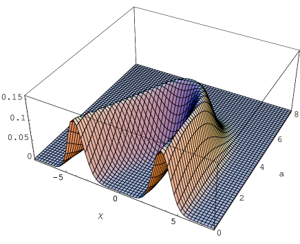
Figure 1: Left, the square of the wave packet $|\psi(\chi,a)|^{2}$ for $C(n)=\frac{{\,\zeta^{n}}}{\,{\sqrt{2^{n}\,n!}}}e^{-|\zeta|^{2}/4}$, $\theta_{0}=\pi/8$ and $|\zeta|=4$. Right, the contour plot of the same figure with the classical path superimposed as the thick solid line.

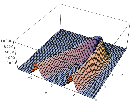
Figure 2: Left, the square of the wave packet $|\psi(\chi,a)|^{2}$ for $C(n)=\frac{n^{2}\,\zeta^{n}}{\,{\sqrt{2^{n}\,n!}}}e^{-|\zeta|^{2}/4}$, $\theta_{0}=\pi/4$ and $|\zeta|=5$. Right, the contour plot of the same figure with the classical path superimposed as the thick solid line.

Now, let us consider the situation using the ontological interpretation of quantum mechanics [29, 30]. This formalism allows us to compare quantum mechanical results with the classical ones. Moreover, since time is absent in quantum cosmology we can recover the notion of time using this approach. In de-Broglie Bohm interpretation of quantum mechanics, the wave function can be written as

$$\Psi=R\,e^{iS},$$ (25)

where $R=R(\chi,a)$ and $S=S(\chi,a)$ are real functions of the scale factor and the scalar field and satisfy the following equations

$$-\frac{1}{R}\frac{\partial^{2}R}{\partial\chi^{2}}+\frac{1}{R}\frac{\partial^{2}R}{\partial a^{2}}+\left(\frac{\partial S}{\partial\chi}\right)^{2}-\left(\frac{\partial S}{\partial a}\right)^{2}+\chi^{2}-a^{2} = 0,$$ (26)

$$\frac{\partial^{2}S}{\partial\chi^{2}}-\frac{\partial^{2}S}{\partial a^{2}}+\frac{2}{R}\frac{\partial R}{\partial\chi}\frac{\partial S}{\partial\chi}-\frac{2}{R}\frac{\partial R}{\partial a}\frac{\partial S}{\partial a} = 0.$$ (27)

Because of the form of the wave packet (11), it is more appropriate to separate the real and imaginary parts of the wave packet

$$\Psi(\chi,a)=x(\chi,a)+iy(\chi,a),$$ (28)

where $x,y$ are real functions of $\chi$ and $a$

$$x(\chi,a) = \sum_{n=\mbox{\footnotesize{even}}}\frac{\displaystyle 1}{\displaystyle H_{n}(0)}\mathrm{Re}[C(n)]\frac{\displaystyle H_{n}(\chi)H_{n}(a)}{\displaystyle\pi^{1/2}2^{n}n!}e^{-(a^{2}+\chi^{2})/2}$$ (29)

$$- \sum_{n=\mbox{\footnotesize{odd}}}\frac{\displaystyle\sqrt{2n+1}}{\displaystyle 2nH_{n-1}(0)}\,\mathrm{Im}[C(n)]\frac{\displaystyle H_{n}(\chi)H_{n}(a)}{\displaystyle\pi^{1/4}\sqrt{2^{n}\,n!}}e^{-(a^{2}+\chi^{2})/2},$$

$$y(\chi,a) = \sum_{n=\mbox{\footnotesize{odd}}}\frac{\displaystyle\sqrt{2n+1}}{\displaystyle 2nH_{n-1}(0)}\mathrm{Re}[C(n)]\frac{\displaystyle H_{n}(\chi)H_{n}(a)}{\displaystyle\pi^{1/4}\sqrt{2^{n}\,n!}}e^{-(a^{2}+\chi^{2})/2}$$ (30)

$$+ \sum_{n=\mbox{\footnotesize{even}}}\frac{\displaystyle 1}{\displaystyle H_{n}(0)}\mathrm{Im}[C(n)]\,\frac{\displaystyle H_{n}(\chi)H_{n}(a)}{\displaystyle\pi^{1/2}2^{n}n!}e^{-(a^{2}+\chi^{2})/2}.$$

These variables are related to $R$ and $S$ through equation (25) as

$$R = \sqrt{x^{2}+y^{2}},$$ (31)

$$S = \arctan\left(\frac{y}{x}\right).$$ (32)

On the other hand, the Bohmian trajectories which determine the behavior of the scale factor and the scalar field, are governed by

$$P_{\chi}=\frac{\partial S}{\partial\chi},$$ (33)

$$P_{a}=\frac{\partial S}{\partial a},$$ (34)

where the momenta correspond to the related Lagrangian (3) are $P_{\chi}=2\dot{\chi}$ and $P_{a}=2\dot{a}$, in the gauge $N=a$. Therefore, the equations of motion take the form

$$2\dot{\chi} = \frac{\displaystyle x\frac{\partial y}{\partial\chi}-y\frac{\partial x}{\partial\chi}}{x^{2}+y^{2}},$$ (35)

$$2\dot{a} = -\frac{\displaystyle x\frac{\partial y}{\partial a}-y\frac{\partial x}{\partial a}}{x^{2}+y^{2}}.$$ (36)

Using the explicit form of the wave packet (29,30), these differential equations can be solved numerically to find the time evolution of $\chi$ and $a$. In the left part of Fig. 3, we have shown the square of the wave packet $|\psi(\chi,a)|^{2}$ for $C(n)=\frac{{\,\zeta^{n}}}{\,{\sqrt{2^{n}\,n!}}}e^{-|\zeta|^{2}/4}$, $\theta_{0}=\pi/8$ and $|\zeta|=7$. In the right part of this figure, we have depicted $\chi(t)$ and $a(t)$ for classical (solid line) and Bohmian (dashed line) trajectories. In fact, the obtained Bohmian quantities versus time ($\chi(t)$ and $a(t)$) coincide well with their classical counterparts. This shows the suppression of the quantum potential along the trajectory due to the coincidence between classical and Bohmian results [13].

Figure 3: Left, the square of the wave packet $|\psi(\chi,a)|^{2}$ for $C(n)=\frac{{\,\zeta^{n}}}{\,{\sqrt{2^{n}\,n!}}}e^{-|\zeta|^{2}/4}$, $\theta_{0}=\pi/8$ and $|\zeta|=7$. Right, plot of $\chi(t)$ and $a(t)$ for classical (solid line) and Bohmian (dashed line) trajectories.

Figure 4: The inverse of classical momentum $P^{-1}$ (dashed line) and the square of the wave packet $|\psi(\chi,a)|^{2}$ along the classical trajectory (solid line) for $C(n)=\frac{{\,\zeta^{n}}}{\,{\sqrt{2^{n}\,n!}}}e^{-|\zeta|^{2}/4}$, $\theta_{0}=\pi/4$ and $|\zeta|=4$ versus $t$.

For the case $\theta_{0}\neq 0$, the momentum is not constant along the classical trajectory $P=2D\sqrt{\sin^{2}(t)+\cos^{2}(t-\theta_{0})}$. In fact, we can also obtain some information about the classical momentum from the shape of the wave packet. For this purpose, we use WKB approximation. In semiclassical approximation, the square of the wave function up to the first order is related to the momentum as

$$|\psi|^{2}\propto\frac{1}{\displaystyle P}.$$ (37)

This equation has a simple interpretation. The low momentum corresponds to the high probability density and vice-versa. Figure 4 shows the square of the wave packet $|\psi(\chi,a)|^{2}$ along the classical (Bohmian) trajectory which is parameterized with time and the inverse of the classical momentum $P^{-1}$ versus time. As it can be seen from the figure, the height of the crest of the wave packet qualitatively shows the variation of the classical momentum along the trajectory. The low consistency between these two quantities is due to the approximate nature of equation (37).

4 Conclusions

We have studied a closed homogeneous and isotropic quantum cosmology model in the presence of a conformally coupled scalar field. We have proposed a new initial condition which results in a complete classical and quantum correspondence. In fact, since the WDW equation is second-order differential equation, we are free to choose the initial wave function and the initial derivative of the wave function. This means that we are also free to choose the expansion coefficients. Since we are interested to have a consistency between classical and quantum solutions, we need to impose a particular relation between the coefficients. In this article, we proposed a particular relation between even and odd expansion coefficients. These coefficients determine the initial wave function and its initial derivative, respectively. In other words, this proposal defines a connection between position and momentum distributions with two properties at the same time. First, they correspond to their classical quantities and second, they respect the uncertainty relation. To quantify the classical and quantum correspondence, we have also studied the situation using de-Broglie Bohm interpretation of quantum mechanics. In fact, the Bohmian trajectories highly depend on the choice of the expansion coefficients and various linear combinations of eigenfunctions lead to different Bohmian trajectories. Therefore, although the inconsistency between classical and Bohmian solutions is natural in most cases, the quantum scenario is not always different from the classical scenario. In this paper, we have tried to construct the wave packets which peak around the classical trajectories and simulate their behavior. We showed that Bohmian positions and momenta coincide completely with their classical counterparts upon choosing arbitrary but appropriate initial conditions. Moreover, using WKB approximation, we qualitatively obtained the classical variation of momentum along the path without utilizing the classical equations of motion.

References

- [1] J. B. Hartle and S. W. Hawking, Phys. Rev. D 28, 2960 (1983); S. W. Hawking, Nucl. Phys. B 239, 257 (1984); in Relativity, Groups and Topology II, Proceedings of the Les Houches Summer School of Theoretical Physics, Les Houches, France, 1983, edited by R. Stora and B. DeWitt, Les Houches Summer School Proceedings Vol. 40 (North-Holland, Amsterdam, 1984).
- [2] A. Vilenkin, Phys. Lett. B 117, 25 (1982); Phys. Rev. D 27, 2848 (1983); 30, 509 (1984); Nucl. Phys. B 252, 141 (1985); Phys. Rev. D 33, 3560 (1986); 37, 888 (1988).
- [3] J. J. Halliwell, Phys. Lett. B 196, 444 (1987).
- [4] A. L. Matacz, Class. Quantum Grav. 10, 509 (1993).
- [5] J. J. Halliwell, Contemporary Physics, 46, 93 (2005).
- [6] B. S. DeWitt, Phys. Rev. 160, 1113 (1967).
- [7] C. Kiefer, Phys. Rev. D 38, 1761 (1988); Phys. Rev. D 38, 1761 (1988); Phys. Lett. B 225, 227 (1989).
- [8] T. Dereli, M. Onder and R. W. Tucker, Class. Quantum Grav. 10, 1425 (1993).
- [9] F. Darabi and H. R. Sepangi, Class. Quantum Grav. 16, 1565 (1999).
- [10] S. S. Gousheh and H. R. Sepangi, Phys. Lett. A 272, 304 (2000).
- [11] S. S. Goushe, H. R. Sepangi, P. Pedram, and M. Mirzaei, Class. Quantum Grav. 24, 4377 (2007).
- [12] P. Pedram, S. Jalalzadeh, Phys. Lett. B, 660, 1 (2008), arXiv: 0712.2593.
- [13] P. Pedram, J. Cosmol. Astropart. Phys. 07, 006 (2008), arXiv:0806.1913.
- [14] P. Pedram, S. Jalalzadeh and S. S. Gousheh, Phys. Lett. B 655, 91 (2007), arXiv:0708.4143.
- [15] P. Pedram, S. Jalalzadeh and S. S. Gousheh, Class. Quantum Grav. 24, 5515 (2007), arXiv:0709.1620.
- [16] H. -J. Schmidt, Phys. Lett. B, 214, 519 (1988).
- [17] J. J. Halliwell and R. Laflamme, Class. Quantum Grav. 6, 1839 (1989).
- [18] J. J. Halliwell, Int. J. Mod. Phys. A 5, 2473 (1990).
- [19] S. W. Hawking and D. N. Page, Spectrum of wormholes, Phys. Rev. D 42 2655 (1990).
- [20] D. N. Page, J. Math. Phys., 32, 3427 (1991).
- [21] J. J. Halliwell, Introductory lectures on quantum cosmology. In Quantum cosmology and baby universes, edited by S. Coleman, J.B. Hartle, T. Piran, and S. Weinberg (World Scientific, Singapore, 1991)
- [22] L. J. Garay, J. J. Halliwell, and G. A. M. Marugán, Phys. Rev. D 43, 2572 (1991).
- [23] S. P. Kim, Phys. Rev. D 46, 3403 (1992).
- [24] C. Barceló and M. Visser, Phys. Lett. B 466, 127 (1999).
- [25] C. Kiefer, Nucl. Phys. B 341, 273 (1990); C. Kiefer, Quantum Gravity (Oxford University Press, Oxford, 2007), 2nd ed.
- [26] G. D. Barbosa, Phys. Rev. D 71, 063511 (2005).
- [27] J. A. de Barros, N. Pinto-Neto, and A. A. Sagioro-Leal, Gen. Relativ. Gravit. 32, 15 (2000).
- [28] P. Pedram, M. Mirzaei and S. S. Gousheh, Computer Physics Communications, 176, 581 (2007).
- [29] P. R. Holland, The Quantum Theory of Motion: An Account of the de Broglie-Bohm Interpretation of Quantum Mechanics, (Cambridge University Press, Cambridge, England, 1993).
- [30] N. Pinto Neto, Quantum Cosmology, VIII Brazilian School of Cosmology and Gravitation (Editions Frontieres, Gif-sur-Yvette, 1996); Found. Phys. 35, 577 (2005), arXiv:gr-qc/0410117.