Far- Ultraviolet Observations of Starburst Galaxies with FUSE: Galactic Feedback in the Local Universe

Abstract

We have analyzed FUSE  (905-1187 Å) spectra of a sample of 16 local starburst galaxies. These galaxies cover almost three orders of magnitude in star-formation rates and over two orders of magnitude in stellar mass. Absorption features from the stars and interstellar medium are observed in all the spectra. The strongest interstellar absorption features are generally blue-shifted by $\sim$ 50 to 300 km s^-1, implying the almost ubiquitous presence of starburst-driven galactic winds in this sample. The outflow velocites increase with both the star formation rate and the star formation rate per unit stellar mass, consistent with a galactic wind driven by the population of massive stars. We find outflowing coronal-phase gas (T $\sim 10^{5.5}$ K) detected via the O VI absorption-line in nearly every galaxy. The O VI absorption-line profile is optically-thin, is generally weak near the galaxy systemic velocity, and has a higher mean outflow velocity than seen in the lower ionization lines. The relationship between the line width and column density for the O VI absorbing gas is in good agreement with expectations for radiatively cooling and outflowing gas. Such gas will be created in the interaction of the hot out-rushing wind seen in X-ray emission and cool dense ambient material. O VI  emission is not generally detected in our sample, suggesting that radiative cooling by the coronal gas is not dynamically significant in draining energy from galactic winds. We find that the measured outflow velocities in the HI and HII phases of the interstellar gas in a given galaxy increase with the strength (equivalent width) of the absorption feature and not with the ionization potential of the species. The strong lines often have profiles consisting of a broad and optically-thick component centered near the galaxy systemic velocity and weaker but highly blue-shifted absorption. This suggests that the outflowing gas with high velocity has a lower column density than the more quiescent gas, and can only be readily detected in the strongest absorption lines. From direct observations below the Lyman edge in the galaxy rest-frame, we find no evidence of Lyman continuum radiation escaping from any of the galaxies in the sample. Moreover, the small escape fraction of light in the center of the strong C II absorption feature confirms the high opacity below the Lyman limit in the neutral ISM. The absolute fraction of escaping Lyman continuum photons is typically $<$1%. This sample provides a unique window on the global properties of local star-forming galaxies as observed in the far-UV and also provides a useful comparison sample for understanding spectra of high redshift star-forming galaxies.

1 Introduction

While $\Lambda$CDM simulations of a universe dominated by dark matter and dark energy have led to a robust understanding of the large scale structure of the universe, many questions remain when studying smaller scales where baryonic physics become important (Robertson et al., 2005; Sommer-Larsen et al., 1999; Benson et al., 2003). Thus, understanding the interplay between a galaxy’s components (e.g. gas, stars, radiation, black holes) and its environment is an important next step for cosmology studies.

In particular, feedback on the surrounding gas-phase baryons provided by massive stars is believed to play a major role in the formation and evolution of galaxies. Starburst driven galactic winds are the most obvious manifestation of these processes. These “superwinds” appear to be omnipresent in galaxies with star formation rates (SFR) per unit area $\Sigma_{\ast}\gtrsim 10^{-1}\,\rm{M_{\odot}\,yr^{-1}\,kpc^{-2}}$ (Heckman, 2003). Locally, these starbursts alone account for roughly 20% of the high-mass star formation and 10% of the radiant energy production (Heckman et al., 2005). Powered by supernovae and stellar winds these outflows drive gas, dust, energy, and metals out of galaxies and possibly into the inter-galactic medium (IGM, Heckman et al., 1998; Veilleux et al., 2005). The higher overall star-formation rates at $z\sim 1$ and above (Bunker et al., 2004; Hopkins & Beacom, 2006) imply that star-formation driven winds are even more important in the early universe. Such winds at high redshift almost certainly had a profound impact on the energetics, ionization, and chemical composition of the IGM (Aguirre et al., 2005).

Lyman break galaxies (LBGs, Steidel et al., 1999) are the most widely studied population of high redshift star forming galaxies as they can be efficiently selected using the Lyman-break dropout technique. Rest frame UV spectroscopy of LBGs have shown that starburst driven galactic winds appear to be a ubiquitous property of LBGs (Shapley et al., 2003). During the cosmological important epoch of $z\sim 2-4$ LBGs constitute a significant (and possibly dominant) fraction of the population of star forming galaxies (Peacock et al., 2000).

Studies of the outflows in star forming galaxies are complicated by their multiphase nature (Strickland et al., 2004). The mechanical energy from the supernovae and stellar winds create an over-pressurized cavity of hot gas at $\sim 10^{8}$ K (Chevalier & Clegg, 1985). The hot gas expands and cools adiabatically as it accelerates into lower pressure regions. Shock fronts form at the interface between the hot outflowing gas and the ambient material (Strickland & Stevens, 2000). Some of this ambient material is subsequently swept up into the outflow itself. Unfortunately, directly studying the hot wind fluid is only possible in a few local galaxies (e.g. Strickland & Heckman, 2007) due to the low emissivity of the hot gas and observational constraints in the hard X-ray band. Observations then of superwinds focus on either material entrained in the wind fluid (e.g. neutral, ionized, molecular gas and dust) or created through the interface between the hot wind and the ambient material (Marcolini et al., 2005).

The coronal gas ($T\sim 10^{5}-10^{6}$ K) observed in galactic winds is of particular importance. This phase is intimately connected to the mechanical/thermal energy that drives the outflows and places important limits on the cooling efficiency of the outflow. The coronal phase is probed through observations of the O VI$\lambda\lambda 1032,1038$  doublet found in the rest frame FUV. Unfortunately, observations of this wavelength regime in LBGs are generally limited by its location deep within the Lyman $\alpha$ forest. Our knowledge of the properties of the winds in LBGs is generally then limited to what can be inferred from the interstellar UV absorption lines longward of Lyman $\alpha$.

Studies of local star-forming galaxies in this wavelength regime have been limited by UV absorption in the Earth’s atmosphere. Hopkins ultraviolet telescope (HUT) observations of star forming galaxies analyzed by Leitherer et al. (2002) probed the 912-1800 Å  regime but with very low spectral resolution. Heckman et al. (1998) studied a large sample of 45 starburst galaxies using the International Ultraviolet Explorer (IUE) with similarly low resolution and wavelength coverage only longward of about 1150 Å. HST UV ($>1215$ Å) spectral studies have also been undertaken (e.g. Vázquez & Leitherer, 2005; Schwartz et al., 2006) although they focus primarily on specific star clusters given the small spectroscopic apertures of HST.

The situation changed however with the launch of the Far-ultraviolet Spectrographic Explorer (FUSE) in 1999. FUSE  provides high resolution spectroscopy with an aperture that is well matched to observing global FUV properties of local star-forming galaxies. Two previous works using overlapping data sets have used FUSE to study dust attenuation in the FUV (Buat et al., 2002) and stellar populations (Pellerin & Robert, 2007). However, while several previous works have studied specific galaxies with FUSE (e.g. Heckman et al., 2001a; Aloisi et al., 2003; Hoopes et al., 2003, 2004; Grimes et al., 2005; Bergvall et al., 2006; Grimes et al., 2006), a study of the global properties of outflows in a representative sample of star-forming galaxies has not previously been undertaken.

In this paper we will focus on the absorption lines produced by the interstellar medium (ISM) and observed in the FUSE  wavebands. We will first introduce our sample selection method and analysis techniques in Section 2. Next we will discuss the outflow velocity distributions of the various ISM absorption features in Section 3.1. Section 3.2 focuses on the different physical origin of the coronal gas as traced by O VI. We then compare the outflow velocities and strengths of the absorption features to the physical properties of the galaxies in Sections 3.3 and 3.4 respectively. Section 3.5 discusses the possible escape of Lyman continuum emission in local starburst galaxies.

2 FUSE Observations

The FUSE satellite is a high resolution spectrometer with sensitivity in the 905 - 1187 Å  range. Four co-aligned prime focus telescopes, each with its own Rowland spectrograph, comprise the four FUSE  channels. Each channel has its own focal plane assembly with four apertures. Only two science apertures are relevant to this work, the low-resolution aperture (LWRS; $30\arcsec\times 30\arcsec$) and the medium-resolution aperture (MDRS: $4\arcsec\times 20\arcsec$). Spectral resolution (full width at half maximum) ranges from about $17{\rm{km\,s^{-1}}}$ for a point source to about $100{\rm{km\,s^{-1}}}$ for a uniform source filling the LWRS. Two channels have an Al+LiF optical coating while the other two are SiC providing sensitivity for the $\sim$990 - 1187 Å  and $\sim$905 - 1070 Å  ranges respectively. The spectra are imaged onto two micro-channel plate (MCP) detectors (1 & 2) each with two sides (A & B). The four channels and two sides to each MCP produce eight individual spectra for every FUSE  observation. Telescope acquisition and guiding is controlled by a fine error sensor which is aligned with the LiF 1 channel for the observations in this paper.

2.1 Sample Selection

One of the primary motivations for this work is to study the properties of O VI  absorption in star-forming galaxies. The O VI  feature is actually a doublet at 1032 and 1038 Å. In our galaxies the feature is optically thin, and the $\lambda$1038 line will be half as strong as the $\lambda$1032 line. Since the weaker $\lambda$1038 line is severely blended with C II$\lambda 1036$  and O I$\lambda 1039$, we do not attempt to measure it in our spectra. Therefore, our sample selection is driven by the desire to pick star-forming galaxies in which we could detect O VI$\lambda 1032$. While O VI$\lambda 1032$  is generally a prominent feature in these galaxies, it can be very broad and is found in a complicated region of the spectra. The wavelength region around O VI$\lambda 1032$  is particularly intricate due to the presence of several other strong features most noteably $\rm{Ly}\-\beta\,\lambda 1025$  and C II$\lambda 1036$. More problematically, Milky Way (MW) O VI  and C II  are strong absorption features that may also fall on the observed redshifted extra-galactic O VI$\lambda 1032$  feature. Therefore, we cut galaxies with systemic velocities $\rm{v_{sys}}<600\,{\rm{km\,s^{-1}}}$ and $1000<\rm{v_{sys}}<1500\,{\rm{km\,s^{-1}}}$ as extragalactic O VI  would then be blended with the strong Milky Way O VI  and C II  features respectively. The two highest redshift galaxies in the original sample were also dropped as the O VI was shifted onto the gap between the LiF channels at $\sim$1090Å. We also require S/N $>4$ in 0.078 Å  bins in the LiF 1A galaxy spectrum. The LiF 1A spectrum is the highest S/N spectrum of the eight spectra that are obtained during every FUSE  exposure. This reduced our sample from the 54 star-forming galaxies we found in the archive to only 15 objects. We have however made an exception for one galaxy, NGC 4214. One of the side-effects of dropping galaxies with $\rm{v_{sys}}<600\,{\rm{km\,s^{-1}}}$ is that we dropped a majority of the lower SFR galaxies found in the archive. In the case of NGC 4214, it is a particularly high quality dataset (S/N=14.6) with sufficiently narrow absorption features so that they are cleanly separated from the MW features. We therefore include NGC 4214 in our sample for a total of 16 galaxies. Table 1 lists the galaxies in our sample along with many of their physical properties.

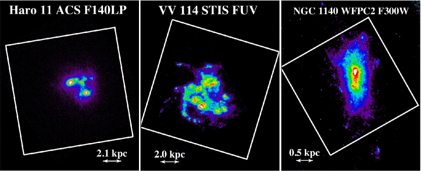
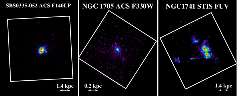
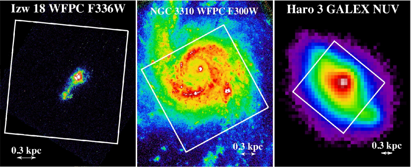
Figure 2: UV or FUV images with FUSE aperture overlay for Haro 11, VV 114, NGC 1140, SBS 0335-052, NGC 1705, NGC 1741, I Zw 18, NGC 3310, and Haro 3. The FUSE  LWRS aperture has been overlaid at the nominal position and orientation for the FUSE observations. The image of Haro 3 is a GALEX NUV observation at significantly lower spatial resolution than observed in the other panels. The overlaid arrows are 5″in length.

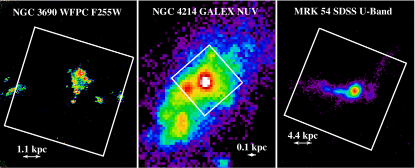
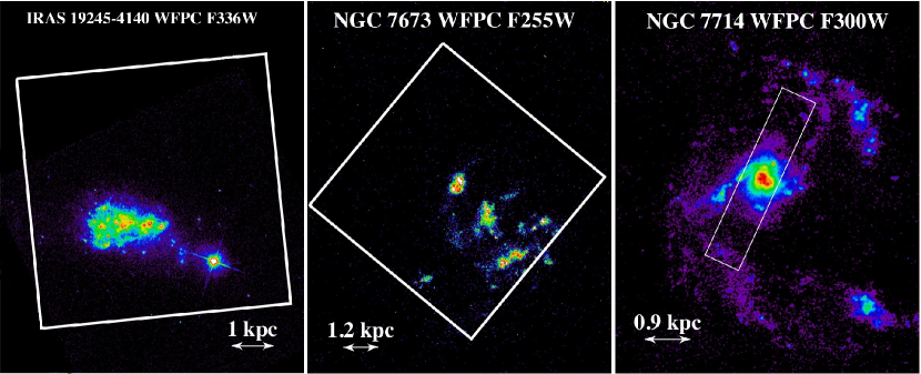
Figure 3: UV images with FUSE aperture overlay for NGC 3690, NGC 4214, Mrk 54, IRAS 19245-4140, NGC 7673, and NGC 7714. The FUSE  LWRS aperture has been overlaid at the nominal position and orientation for the FUSE observations. The images of NGC 4214 (GALEX NUV) and Mrk 54 (SDSS U-band) are at significantly lower spatial resolutions than observed in the other panels.

The FUSE  apertures for these observations are generally pointed directly at the location of the most intense SF in every galaxy. As the FUV emission of most of the starbursts in the sample is strongly peaked near the galaxy center, the LWRS aperture includes the majority of the FUV emission for each galaxy. We are therefore probing the FUV properties of the entire galaxy, similar to observations of high redshift LBGs. The lone MDRS pointing, NGC 7714 has a compact nuclear starburst so that the majority of FUV emission of the galaxy is enclosed even in the smaller aperture. We have overlaid the FUSE aperture and orientation on FUV or UV images for 15 of the galaxies in this sample in Figures 2 and 3. Tol 0440-381  has been excluded as a UV image of that object is not available. All of the images in this sample are continuum UV images although the majority are at significantly longer wavelengths than our FUSE  spectroscopy. Most of the images are HST WFPC using either the F255W ($\lambda_{c}=2599$ Å), F300W ($\lambda_{c}=2987$ Å), or F336W ($\lambda_{c}=3344$ Å) filters. All but three of the images are from high spatial resolution HST instruments with the exception of the low resolution images of Mrk 54 (SDSS U-Band), NGC 4214 (GALEX NUV), and Haro 3 (GALEX NUV). A logarithmic image scaling has been used to highlight the various features of these galaxies although it does somewhat misrepresent the relative strength of the central features. Specifically, only NGC 3310 has significant extended emission outside of the central regions of the FUSE aperture.

The selected galaxies in our sample represent a wide range in galaxy types and properties. The galaxies span over two orders of magnitude in stellar mass and nearly three orders of magnitude in SFR. We have included several dwarf galaxies (e.g. I Zw 18, NGC 4214, NGC 1705), spirals (NGC 3310, NGC 7714), compact ultraviolet luminous galaxies (UVLG; VV 114, Haro 11, Mrk 54), and highly IR-luminous mergers (NGC 3690, VV 114). The UVLGs are of particular interest due to their strong similarities to LBGs in terms of their masses, UV luminosities, and UV surface brightnesses (Heckman et al., 2005; Hoopes et al., 2006; Overzier et al., 2008).

2.2 Data Reduction

We have chosen to use a consistent data reduction method throughout the sample aimed at maximizing S/N. This method involves several extra analysis steps but provides superior data quality compared to the standard data reduction method for the targets in our sample. While some of the observations have high S/N ratios in the LiF channels, the lower effective area SiC channels are almost always relatively low S/N. Our study focuses principally on the LiF channel data but we use the SiC data for measuring the very strong C III$\lambda 977$ absorption line and investigating possible escaping Lyman continuum emission.

The first step was to run all raw exposure data through the CalFUSE 3.1.8 data pipeline to produce intermediate data (IDF) files. We then extracted all eight flux calibrated spectra for every FUSE  exposure. See Dixon et al. (2007) for a complete discussion of the calibrations and corrections applied to the data. Mirror misalignment and thermally-induced rotations of the spectrograph gratings cause small zero point shifts in the wavelength calibration. Therefore we cross calibrate the flux calibrated exposures to determine the individual zero-point wavelength shifts. Given that most of our observations are relatively low S/N spectra of extended sources it is difficult to accurately determine many of these wavelength offsets. We subsequently have chosen conservative offsets. A histogram of the offsets used for all of the individual exposures in shown in Figure 1. The majority of the offsets are $<0.013$ Å  ($<4\,{\rm{km\,s^{-1}}}$) which is significantly less than the wavelength inaccuracies caused by localized distortions of the detector (0.025 Å  $\sim 8\,{\rm{km\,s^{-1}}}$).

After determining the wavelength offset for each individual spectra we retroactively apply the correction to the individual IDF files. We also examine the count rates of the individual exposures and throw out the exposures with significant discrepancies. These variations are usually caused by misalignment of a mirror on the target. The IDF files for each exposure are then combined to create one total IDF file for each channel. We then re-extract a combined flux calibrated spectrum which also has the zero-point wavelength corrections applied. More importantly, however, the longer, combined IDF files allow the CalFUSE pipeline to do an improved background subtraction. In particular, the pipeline fits the various backgrounds (e.g. detector, airglow, and geo-coronal scattered light). For the shorter, individual exposures it simply scales the background files by exposure time when extracting flux calibrated spectra. As there can be significant background variations, exposure time scaling can introduce significant background subtraction errors. The backgrounds dominate the signal for many of these spectra so that errors in the background subtraction introduces systematic offsets in the flux scale. Even when using background fitting, these systematic offsets can still be seen in many of the low S/N SiC spectra.

In order to minimize the detector background, we have extracted our spectra using the smaller, point source detector regions (Dixon et al., 2007) for all objects in our sample with the exception of NGC 1705, NGC 3310, and NGC 4214. A visual examination of the 2-D detector images shows that these three galaxies have source counts falling outside of the point source aperture. These are the three highest flux galaxies within our sample. Figure 2 suggests that at least for NGC 3310, the galaxy has considerable extent within the FUSE  aperture. By using the smaller point source region for the remaining 14 galaxies we include the same amount of source flux but minimize the included background.

For galaxies which contain a significant fraction of night only data, we have thrown out the daytime data. Significant airglow features contaminate the day time spectra and are best avoided whenever possible. Table 2 lists the FUSE  observational data for all of the galaxies included in our sample.

2.3 Data

The SiC 2A, LiF 1A, and LiF 2A spectra for every galaxy in our sample are shown in Figures 4 - 19. These channels cover most of the wavelength regime between 920 - 1180 Å. We use LiF 2B for these panels instead of LiF 1B as it is rarely affected by the “worm”. The “worm” is depression in the observed flux that can span over 50 Å in length (Dixon et al., 2007). Shadowing by a grid of quantum efficiency wires where the secondary focus falls above the detectors and close to the location of the wires causes these observed drops in flux. This feature is seen in almost all of the LiF 1B spectra in our sample but does not affect any of the other channels.

Most of the common MW, galactic, and airglow features are marked on these figures. The galactic absorption lines probe the stellar population, interstellar medium (ISM), and outflowing gas. $\rm{H_{2}}$, usually of MW origin, is present in many of the galaxies and is a significant hurdle in identifying and fitting many of the weaker ISM absorption features.

2.3.1 Gaussian Fits

We have fit absorption lines to most of the most prominent features using the IRAF  (Tody & Fitzpatrick, 1996) tool specfit (Kriss, 1994). We have not attempted to fit every possible feature but have instead focused on the strongest, separable lines that we positively identify (this can be particularly difficult in galaxies contaminated by MW $\rm{H_{2}}$). Each line was fit using a freely varying powerlaw for the continuum and a symmetric gaussian absorption line. When absorption lines are blended (e.g. O I $\lambda$989 and N III $\lambda$990) we fit them simultaneously. Due to the differences in the redshifts of the galaxies (and hence differing degrees of blending or contamination by lines due to the Milky Way), it was not possible to consistently define the spectral windows over which the adjacent continuum was fit for any given absorption feature.

We note that the compact UV sizes of most of these galaxies implies that the velocity resolution in our spectra willi typically be roughly $20{\rm{km\,s^{-1}}}$ (FWHM). The worst resolution will be for NGC 3310, which based on its angular size we estimate will be about $60{\rm{km\,s^{-1}}}$. In all cases, the observed absorption-lines are well-resolved.

For the majority of absorption lines we have used the LiF channels to make two independent measurements of the equivalent width, velocity, and full-width half-maximum (FWHM). For lines with only one measurement, the line either fell in the gap between LiF channels or was in the region (1125-1160Å) affected by the worm on the LiF 1B channel. We have generally ignored the SiC channels above 1000 Å  due to their lower S/N. The results of our fits are listed in Tables 3 - 15.

The listed statistical errors are $1\sigma$ and are calculated from the minimization error matrix which is re-scaled by the reduced $\chi^{2}$ value (Kriss, 1994). Systematic errors are probably not large in the FWHM measurement but may be important to the equivalent width and centroid velocity. The equivalent width determination is largely a problem for saturated lines in low S/N spectra. Background over-subtraction is a common problem for these spectra so it is difficult to determine the continuum level and flux zero point. Systematic wavelength calibration errors exist and are particularly hard to quantify for our extended sources using the LWRS aperture. Dixon et al. (2007) suggest that they are order 10 $\rm{km\,s^{-1}}$  which seems consistent with the observed variations in our results. A comparison of the derived parameters for features with data on two LiF channels shows broad agreement, generally well within the $1\sigma$ error bars as expected. In these cases, we have used the error weighted value to create a single measurement for the analysis that follows.

Close up plots of six strong absorption features for all 16 galaxies are shown in Figures 20 - 35. The plots focus on the ISM absorption lines observed in almost all of the spectra, specifically O VI$\lambda 1032$, C II$\lambda 1036$, C III$\lambda 977$, O I$\lambda 989$, N II$\lambda 1084$, and O I$\lambda 1039$. We have displayed these spectra even when the absorption feature was not observed. MW ISM contamination, $\rm{H_{2}}$, airglow, instrument coverage gaps, and signal quality play an important role in which features are actually detected. Line blending is also important most particularly for O I$\lambda 989$  as it falls right next to the strong N III$\lambda 990$  feature.

Another potentially problematic blending is C III$\lambda 977$  with O I$\lambda 976$. However, we have checked the significance of the contamination by modeling the O I$\lambda 976$  line using our gaussian fits to O I$\lambda 1039$. From Morton (1991) we expect O I$\lambda 976$  to be a factor of 2.7 weaker than O I$\lambda 1039$  for an optically thin feature. In Figure 36 we have overlayed an O I$\lambda 976$ absorption feature with the same velocity and FWHM as the O I$\lambda 1039$  profile but we have lowered the equivalent width by a factor of 2.7 for NGC 1140 and NGC 3310. As shown in these plots, this feature is significantly weaker than the observed C III$\lambda 977$  profile. Fitting these profile with the O I$\lambda 976$  contribution does not change the derived equivalent widths, centroid velocities, and FWHMs in a significant manner. The largest percentage change is seen in the FWHMs which lower by 12 and 11 $\rm{km\,s^{-1}}$  for NGC 1140 and NGC 3310 respectively. This is only 25% of the $1\sigma$ statistical error. We therefore conclude that the weak O I$\lambda 976$  is not significantly affecting our fits to the C III$\lambda 977$  profile.

The strength of the absorption lines varies widely across the sample. As discussed in our previous work Grimes et al. (2006) and Grimes et al. (2007), most of the strong absorption line profiles are non-gaussian. The absorption profiles frequently show significant structure suggesting that in many cases these are an aggregate profile representing multiple absorbers spread throughout the galaxy’s ISM and starburst driven outflow. Many of the profiles are asymmetric, with stronger absorption on the blueward side of the line core. This is consistent with absorbing gas entrained in and accelerated by an outflowing wind fluid.

In our previous work we have successfully modeled many of the stronger lines with two gaussian component fits. Physically, for both Haro 11  and VV 114  the stronger gaussian was associated with the host galaxy ISM while the blueshifted gaussian represented outflowing gas at several hundred $\rm{km\,s^{-1}}$. For this work, covering a wide range of galaxy star formation rates and data quality, a multiple component fit is not feasible. Therefore, we have used two additional methods to study the strongest absorbers in our sample.

2.3.2 Apparent Optical Depth Method

For O VI$\lambda 1032$  we use the apparent optical depth method as described in Sembach et al. (2003). This method assumes that the O VI  absorption features are not saturated - which is consistent with the observed O VI  profiles. The apparent column density as a function of velocity is given by

$${\rm N_{a}}(\nu)=\frac{\tau_{\rm a}(\nu)}{f\lambda}\frac{m_{e}c}{\pi e^{2}}=3.768\times 10^{14}\frac{\tau_{\rm a}(\nu)}{f\lambda({\rm\AA})}$$ (1)

where

$$\rm{\tau_{a}(\nu)=-\ln[I_{obs}(\nu)/I_{0}(\nu)].}$$ (2)

$\rm{I_{0}(\nu)}$ is the continuum intensity while $\rm{I_{obs}(\nu)}$ is the observed line intensity. The O VI  line profiles in Figures 20 - 35 show that the line is clearly resolved when present. Therefore we can obtain the column density by integrating over velocities as $\rm{N}=\int\rm{N(\nu)}d\nu=\int\rm{N_{a}(\nu)}d\nu$. The apparent optical depth method also allows us to calculate the velocity centroid and line width using $\bar{\nu}=\int\nu\tau_{\rm a}(\nu)d\nu/\int\tau_{\rm a}(\nu)d\nu$ and $b=[2\int(\nu-\bar{\nu})^{2}\tau_{\rm a}(\nu)d\nu/\int\tau_{\rm a}(\nu)d\nu]^{\text@frac{1}{2}}$ respectively. Table 19 lists our results.

In our previous work we have calculated the O VI  parameters for VV 114  and Haro 11  from gaussian fits. For VV 114  these two methods are in excellent agreement as we had found $\rm N_{O\,VI}$  $\sim 2.0\times 10^{15}\,{\rm cm^{-2}}$ while we now calculate $\rm N_{O\,VI}$  $\sim 2.2\times 10^{15}\,{\rm cm^{-2}}$ using the apparent optical depth measurement. These results are consistent because the O VI  profile shape is approximately gaussian for VV 114 (see Figure 21). We find however a larger discrepancy for Haro 11  with $\rm N_{O\,VI}$  $\sim 4.2\times 10^{14}\,{\rm cm^{-2}}$ and $\rm N_{O\,VI}$  $\sim 8.0\times 10^{14}\,{\rm cm^{-2}}$ for the gaussian and apparent optical depth methods respectively. For Haro 11  (Figure 20), a multicomponent profile is observed. In this case the apparent optical depth method better includes the extended blue wing. We also now derive a larger absorption line width and a more blueshifted velocity centroid, consistent with a significant contribution from the extended blue wing of the absorption profile. The apparent optical depth method provides a significant improvement over gaussian profiling for O VI  and is applicable as O VI  is not saturated or blended significantly with other lines (partly due to our sample selection). Table 19 does not include four galaxies. For NGC 1140, I Zw 18, and IRAS 19245-4140  we do not positively detect O VI  absorption. In Tol 0440-381  the O VI is a broad, shallow feature making it impossible to reliably estimate the velocity limits over which the above integral should be performed.

2.3.3 Non-parametric Equivalent Widths

Several other strong absorbers exist in the spectra of these star-forming galaxies, specifically C II$\lambda 1036$, C III$\lambda 977$, and N II$\lambda 1084$. Unlike O VI$\lambda 1032$  however, these lines are frequently saturated at line center and therefore we are unable to apply the apparent optical depth method. We therefore measure the equivalent widths and velocity centroids of these lines using the IRAF  (Tody & Fitzpatrick, 1996) tool splot. The procedure subtracts a user defined linear continuum and sums the resulting flux to calculate the equivalent width. The comparably strong O I$\lambda 989$  and N III$\lambda 990$  lines are frequently blended, so these lines have been excluded from the procedure. Our results are listed in Table 20. These lines are frequently saturated, particularly C III  and C II , so the equivalent widths are essentially just a measure of how broad the absorption feature is.

We have also compared the non-parametric equivalent widths, centroids, and widths with those derived from our previous gaussian fits in Section 2.3.1. There is broad agreement for the derived values using the C II  and N II features. The principal outliers are the C II  centroid velocities for some of the galaxies with higher SFR ($>$ a few $\rm 10^{10}\,L_{\odot}$) where the outflow velocities are found to be higher from the non-parametric fits. In the case of C III, there is a systematic shift to higher outflow velocities for the non-parametric values. This is observed in almost all of the galaxies in our sample not just in the galaxies with higher SFR. These findings are consistent with our motivation for using a non-parametric method to measure these absorption features. Specifically, as line strengths increase the absorption features are found to be increasingly non-gaussian and blue-asymmetric.

For the analysis that follows unless otherwise stated, we use these non-parametric measurements for the C III, C II, and N II  features. For O VI  we use the results derived from the apparent optical depth method and for the remaining lines we use the gaussian data.

3 Discussion

This paper is intended to be a general study of the FUV properties of starburst galaxies. As stated previously, we will focus on the strongest ISM absorption features in order to include the majority of galaxies in our sample. In particular, we will focus on the following lines: O VI$\lambda 1032$, C III$\lambda 977$, S III$\lambda 1012$, N II$\lambda 1084$, C II$\lambda 1036$, O I$\lambda 1039$. These lines are detected and measured throughout most of our sample. They also represent three different phases of the ISM - coronal (O VI), HII (C III, S III, N II) and HI (C II, O I).

3.1 Outflow Velocity Distributions

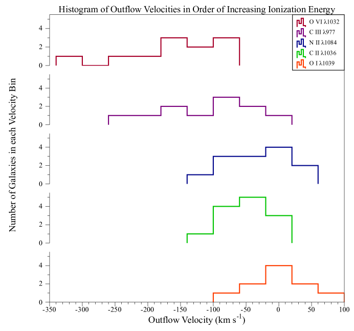
Figure 37: Velocity Outflow Histogram for Prominent Absorption Lines: Outflows are observed for all of the absorption features except O I$\lambda 1039$. Observed outflow velocities are significantly higher for O VI  and C III.

In Figure 37 we have plotted histograms of the relative velocities for the strongest of these absorption features. These lines are listed in order of increasing ionization potential. With the exception of the neutral oxygen ion, the other absorption features show the presence of outflows ranging up to a few hundred $\rm{km\,s^{-1}}$. As the ionization state increases the lines generally have larger outflow velocities. The sole exception is C II  which is mildly more blueshifted than N II. The C III  and O VI  lines however are significantly more blueshifted than the two lower ionization state ions.

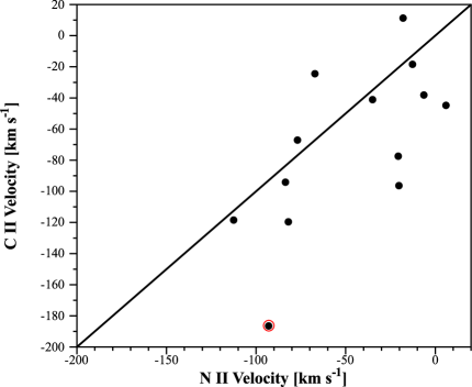
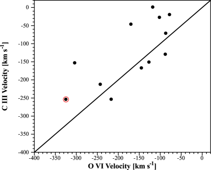
Figure 38: Outflow Velocity Comparison: The plot on the left shows the C II$\lambda 1036$  versus N II$\lambda 1084$  velocities while the right displays the C III$\lambda 977$  versus O VI$\lambda 1032$  velocities. C II  and O VI  are generally more blueshifted than the N II  and C III  features respectively. The lines represents $\rm{v_{x}=v_{y}}$ for both plots. NGC 3310 (which has unusually large outflow velocities for its mass and star formation rate) is denoted by a red circle.

In Figure 38 we have directly compared the velocities of these absorption features. The left panel shows C II  versus N II outflow velocity while the right panel is C III  versus O VI. For the majority of galaxies in our sample, C II  is clearly more blueshifted than N II. Similarly, O VI  has an higher outflow velocity than C III. This confirms the pattern seen in Figure 37.

As we have previously discussed, the O VI  line (unlike C III, C II, and N II) is not saturated for any of the galaxies in our sample. Moreover, an examination of the O VI  profile shape suggests a different origin for this feature. The strongest part of the O VI profile is blueshifted, and the absorption at or near the galaxy systemic velocity is weaker. In contrast, the C III, C II, and N II  lines are broad with extended blueshifted wings, and have the strongest absorption (the line core) at or near the galaxy’s systemic velocity. Furthermore, the maxiumum outflow speed (defined by the blueward extent of the absorption-line profile) is similar for O VI  and C III.

Thus, the gas traced by the O VI  line appears to be primarily in the outflow rather than in the quiescent ISM, while the lower ionization lines are produced by both. This difference is not surprising since O VI has a much higher ionization potential and is produced in significantly higher temperature gas. We will discuss this further in Section 3.2.

Several previous studies have suggested that the measured outflow velocities increase with the ionization potential of the species in starbursts. Vázquez et al. (2004) used HST STIS spectroscopy of NGC 1705 (also represented in our FUSE  sample) and found that several high ionization lines had higher outflow speeds. Schwartz et al. (2006) similarly used HST STIS to observe starclusters in 17 star-forming galaxies (including NGC 3310 and NGC 1741 also in this work). While C II$\lambda 1335$, Al II$\lambda 1671$, and Si II$\lambda 1260$  all trace the neutral hydrogen phase, they found evidence that C II$\lambda 1335$  had higher outflow speeds than the two slightly lower ionization features. We also noticed similar behavior previously when studying the FUSE  observations of Haro 11 (Grimes et al., 2006, Haro 11  is also in this sample). Schwartz et al. (2006) suggest that this could be explained by less dense, hotter gas escaping the starburst region and expanding at a faster speed than the denser, lower ionization gas.

This picture appears to be different than what is observed in high redshift Lyman break galaxies (LBGs). Pettini et al. (2002) have examined high quality spectra of the lensed LBG, MS1512-cB58. They found the same velocity distributions for both the low and high ionization features. Using a composite LBG spectrum, Shapley et al. (2003) also found similar outflow velocities for both the lower and higher ionized absorption features.

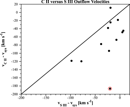
Figure 39: C II$\lambda 1036$  versus S III$\lambda 1012$ velocities. While S III  has a significantly larger ionization energy (23.3 eV) than C II$\lambda 1036$  (11.3 eV), higher outflow velocities are observed in C II. The line represents $\rm{v_{CII}=v_{SIII}}$ in both plots. NGC 3310 (which has unusually large outflow velocities for its mass and star formation rate) is denoted by a red circle.

As discussed previously C III , with an ionization potential of 24.4 eV, has significantly higher outflow velocities than C II  (11.3 eV), N II  (14.5 eV), and O I. This is then consistent with the idea that higher ionization lines have higher outflow velocities. On the other hand, the lower ionization C II  has a slightly higher outflow velocity than N II (e.g. left panel of Figure 38). To study this further we have plotted the C II$\lambda 1036$  versus S III$\lambda 1012$  velocities (Figure 39). S III  has a much higher ionization potential (23.3 eV) than C II  but is a weaker feature. It is not saturated and is well fit by a gaussian model (unlike the stronger features). C II, C III  and N II  all have significantly higher outflow velocities than S III , which is not consistent with an increase of velocity with ionization energy.

In Tables 3 - 18 we listed the absorption features in order of decreasing values of $\log(\lambda fN/N_{H})$. The oscillator strength ($f$) values are from Morton (1991) and solar relative abundances are assumed for $N/N_{H}$. While the majority of the galaxies in our sample do not have solar metallicity (Table 1), this is still a useful predictor of the relative strengths of the absorption features. With the exception of O VI (which we have already argued has a different physical origin than the other ISM absorption features) the values of the equivalent widths follow decreasing $\log(\lambda fN/N_{H})$ (see also Table 20). It is particularly striking that our previous ordering of outflow velocities follows the same general trend as the line strengths. Both outflow velocities and line strengths decrease from C III, C II, N II, to O I$\lambda 1039$.

An examination of the line profiles show that the stronger lines have extended blue absorption wings. In fact, these extended absorption wings were our prime motivation in using a non-parametric method for measuring the equivalents widths and centroid velocities (Section 2.3.3) of the strongest features. This was not necessary for the weaker lines like O I$\lambda 1039$  and S III$\lambda 1012$ which are well fit by gaussian modeling. As the absorption lines increase in strength, the extended blue wing in the absorption-line profile becomes more and more conspicuous. The simplest explanation for this is that the high velocity outflowing gas has a lower column density than the more quiescent gas in the ISM. We therefore only detect the fastest moving gas in the strongest absorption features. This explanation is consistent with the observations of the LBG cB58 where the stronger lines span progressively broader ranges in velocity (Pettini et al., 2002). It also explains the higher outflow speeds for C II$\lambda 1335$  relative to Al II$\lambda 1671$  and Si II$\lambda 1260$  (Schwartz et al., 2006) as C II$\lambda 1335$  is the strongest feature. Lastly, in the work by Vázquez et al. (2004), the lines with the highest measured equivalent widths are preferentially those with the highest ionization energies. This result thus appears to be consistent throughout a wide range of galaxy types and absorption features.

This result is particularly relevant to outflow velocities derived in other wavelength regimes. For example, the Na I$\lambda\lambda 5890,5896$  doublet has $\log(\lambda fN/N_{H})=-1.94$, similar to N II$\lambda 1084$. This suggests that observations of local outflows using Na I  absorption are not biased by measuring lower ionic states than the FUV and UV measurements of higher ionization absorption lines. The derived outflow velocities should be consistent with those of other similarly strong absorption features in the neutral and ionized gas. This could strengthen studies comparing observations of Na I absorption in local galaxies with the properties of outflows observed in LBGs. Unfortunately, there is only one galaxy in our sample having published data on the Na I  absorption feature: NGC 4214 (Schwartz & Martin, 2004). In this case the agreement is good: they find an outflow speed of 23 ${\rm{km\,s^{-1}}}$, while we find speeds ranging from 0 to 58 ${\rm{km\,s^{-1}}}$ depending on the particular line.

3.2 Origin of O VI Absorption

The O VI line is a particularly interesting one due to its potential importance in radiative cooling and the relatively narrow temperature range over which it is a significant (e.g. $\rm T\sim 10^{5}-10^{6}\,K$). As we have discussed, the kinematics of the coronal gas as traced by the O VI absorption line are different from that seen in the cooler gas. In particular, O VI  is the most blueshifted ion and (on kinematic grounds) is located primarily in the outflowing gas and not in galaxy itself.

Several previous papers have studied O VI in specific galaxies, e.g. NGC 1705 (Heckman et al., 2001a), VV 114  (Grimes et al., 2006), and Haro 11  (Grimes et al., 2007). They attributed the production of O VI  to the intermediate temperature regions created by the hydrodynamical interaction between hot outrushing gas and the cooler denser material seen in H$\alpha$ images. Such a situation is predicted to be created as an overpressured superbubble accelerates and then fragments as it expands out of the galaxy and again as the wind encounters ambient clouds in the galaxy halo.

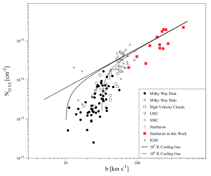
Figure 40: Column density vs. line width for a wide variety of O VI absorption line systems including galactic disk and halo, high velocity clouds, starburst galaxies, and the IGM. The two dashed lines indicate the predictions for radiatively cooling gas for assumed temperatures of $\rm{T_{OVI}=10^{5},\,10^{6}~{}K}$. This plot is originally from (Heckman et al., 2002). The star-forming galaxies from this work have been added and extend the relationship to much higher column densities.

Heckman et al. (2002) derived a simple and general relationship between the O VI  column density and absorption line width which will hold whenever there is a radiatively cooling gas flow passing through the coronal temperature regime. They showed that this simple model accounted for the properties of O VI  absorption line systems as diverse as clouds in the disk and halo of the Milky Way, high velocity clouds, the Magellanic Clouds, starburst outflows, and some of the clouds in the IGM. Using the the values found in Table 19, in Figure 40 we have updated the original plot from Heckman et al. (2002). Our results for the O VI  measured for the galaxies in our sample are fully consistent with the model predictions. The fact that starbursts tend to lie at slightly lower column density than the model predicts is not surprising, given that the model is so generic and idealized (the exact value of the coefficient relating column density to flow speed depends weakly on the exact nature of the flow, as described in Heckman et al. (2002). We conclude that O VI  traces radiatively cooling gas produced in an interaction between the hot outrushing gas seen in X-rays and the cool clouds seen in H$\alpha$ emission, and that this is is a generic feature of starburst galaxies.

In the case of NGC 1705 Heckman et al. (2001a) showed that the overall mass of the coronal phase gas was significantly smaller than the lower ionization material (by about two orders-of-magnitude). They showed that this is consistent with the picture in which this gas is rapidly cooling (it is transitory). Following Heckman et al. (2001a) we can make a rough estimate of the gas mass for our sample of galaxies. This mass is simply the product of the O VI  column density, the surface area of the O VI region, and the inverse ratio of O VI  to total column. The most physically plausible idealized geometrical model is one in which the coronal gas traces the interface between spherically expanding wind and the ambient gas in the galaxy halo. Grimes et al. (2005) found that the wind radius as traced in soft X-ray emission increased systematically with both the star formation rate and galaxy stellar mass. Over the range spanned by our sample, the radius would range from about 0.7 kpc to about 10 kpc. The conversion from O VI  to total column density would be factor of about $10^{4}$ for gas in collisional ionization equilibrium at $T=3\times 10^{5}$ K and with a solar oxygen abundance. The implied masses of coronal gas range from about $10^{6}M_{\odot}$ for the dwarf starbursts like NGC 1705, NGC 4214, and Haro 3 to about $10^{8}M_{\odot}$ for the most powerful starbursts like VV 114 and NGC 3690.

It is also interesting to note the lack of O VI  emission in the sample. While weak O VI  emission is observed in Haro 11  (Bergvall et al., 2006; Grimes et al., 2007) there is no convincing evidence for it in any of the other galaxies in this sample. Very broad (few thousand km s^-1) O VI  emission features appear in a few of the spectra, consistent with stellar winds in the population of O stars (Pellerin et al., 2002). As O VI  emission is the dominant cooling mechanism for coronal gas, the general lack of observed emission implies that radiative cooling is not significantly impeding the growth of the outflow. This is true even in the case of Haro 11 Grimes et al. (2007). They suggested that the O VI  emission may not be from coronal gas cooling but instead could be resonant scattering of far-UV continuum photons from the starburst off O VI  ions in the backside of the galactic wind traced by the blueshifted O VI absorption.

3.3 Dependence of Outflow Velocities on SFR & Stellar Mass

In Grimes et al. (2005) we analyzed Chandra  data of star-forming galaxies ranging from dwarf starbursts to ultra-luminous infrared galaxies (ULIRGs). We showed that the temperature of the hot gas was not dependent upon the galaxy’s SFR. The thermalized X-ray gas is thought to be produced in a reverse shock between the hot out-rushing wind fluid and the ambient material (Strickland & Stevens, 2000), and its temperature is then determined by the wind outflow velocity. Since a relationship between X-ray temperature and SFR was not observed, it follows then that the wind outflow velocity does not depend on the SFR.

In contrast, Martin (2005), Schwartz et al. (2006), and Rupke et al. (2005) have shown that the outflow speed measured in absorption lines does depend on the SFR. Martin (2005) and Rupke et al. (2005) observed outflows in luminous infrared galaxies (LIRGs) and ULIRGs using the NaI D doublet and found that the outflow velocities increased with the SFR up to values of SFR of a few tens M_⊙ yr^-1. At higher SFRs (extending up to several hundred $\rm M_{\odot}\,yr^{-1}$), the relation appears to saturate with the outflow velocities no longer increasing. Similarly, in the STIS starburst sample discussed in Section 3.1 Schwartz et al. (2006) also found that the outflow speeds increased with the SFR below $\sim$10 $\rm M_{\odot}\,yr^{-1}$.

Martin (2005) suggests that the simplest explanation is that there is not enough momentum carried by the wind fluid in the lower SFR galaxies, so that the winds are unable to accelerate the entrained absorbing material up to the velocity of the wind fluid itself. The relation between SFR and the outflow speed seen in the absorption-lines saturates at about 500 ${\rm{km\,s^{-1}}}$ (Martin, 2005) and this is reached at starburst luminosities $sim$ few $\times 10^{11}L_{\odot}$. If the X-ray emission in galactic winds arises in wind shocks, the observed temperatures of $kT_{X}\sim$ 0.3 to 0.7 keV correspond to wind shock speeds of $\sim$ 500 to 800 ${\rm{km\,s^{-1}}}$ (Grimes et al., 2005). This is then compatible with the idea that at sufficiently high SFR (high enough wind momentum) the entrained absorbing gas has been accelerated to near the wind speed.

We can check these results with our data. To that end, we will use the sum of the IRAS IR and FUSE  UV luminosity as our tracer of the SFR (see Table 1). The UV luminosity is based on the continuum flux at 1150 Å and is corrected for Milky Way extinction. The combined UV and IR luminosity provides a reasonable estimate of the intrinsic UV flux of the galaxy, and thus traces recent SF.

Martin (2005) also found that the outflow velocity increased with the rotational speed of the galaxy. This suggests that faster outflows are found in more massive galaxies. We check this correlation using the near-infrared luminosity of the galaxy ($\rm L_{K}$) as a proxy for stellar mass. The K-Band Cousins-Glass-Johnson (CGJ) luminosities are derived from the 2MASS atlas (Jarrett et al., 2003). The 2MASS K and J Band fluxes given in the catalog were converted to K-Band CGJ using the transformations from Carpenter (2001). We expect the K-band luminosity to trace the stellar mass to a factor of roughly two (e.g. Leitherer & Heckman 1995; Bell & de Jong 2001; Dasyra et al. 2006).

We have made no attempt to correct for the viewing angle dependence of the outflow velocity. This is primarily a practical decision as we do not have a robust way of obtaining the orientation of the outflow in these galaxies. While this will increase the scatter in our outflow velocity plots, sample selection effects probably minimize the resulting damage. In particular, an edge-on spiral galaxy would not have had enough FUV flux to meet our S/N requirements as the disk heavily absorbs the nuclear starburst (e.g. M 82). Spiral arm features are apparent for several of the galaxies in our sample (Figures 2 and 3) suggesting that we are observing the galaxies roughly face-on, and hence roughly along the expected outflow direction. Several other of the galaxies have irregular morphologies. In these irregular galaxies it is not at all apparent how inclination angle would be defined. As an example, Haro 11  has several regions of intense SF which high resolution HST ACS imaging suggests could be driving multiple outflows.

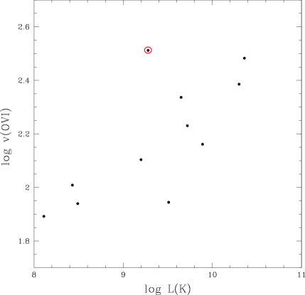
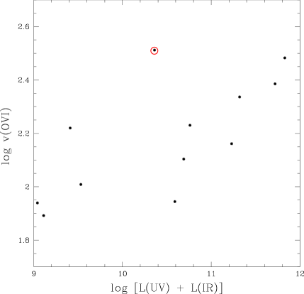
Figure 41: The log of the O VI  outflow velocities in km/s versus the log of the K-Band and IR+UV luminosities (in $L_{\odot}$). These are roughly proportional to the stellar mass and star formation rate respectively. NGC 3310 (which has unusually large outflow velocities for its mass and star formation rate) is denoted by a red circle.

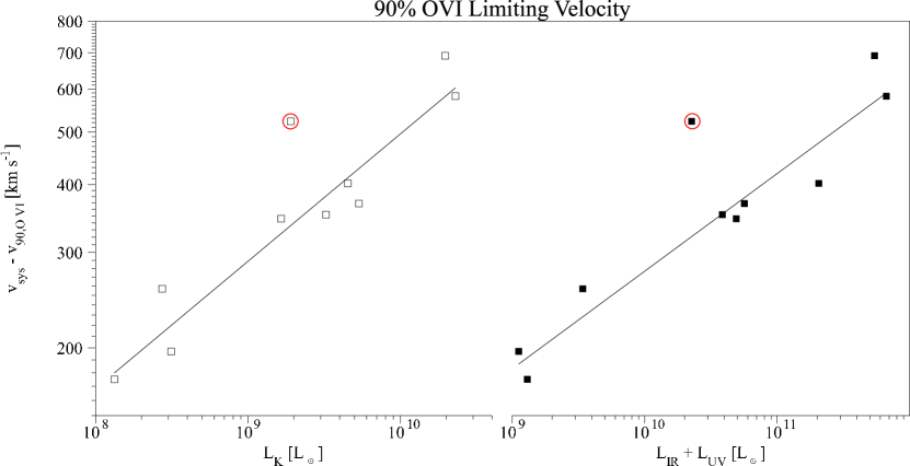
Figure 42: Same as Figure 41, except that here we plot the ‘maximum’ outflow velocity. This is defined so that 90% (10%) of the absorbing column of gas is to the red (blue) of the velocity. See text for details. NGC 3310 (which has unusually large outflow velocities for its mass and star formation rate) is denoted by a red circle.

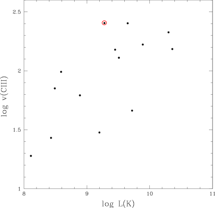
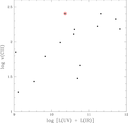
Figure 43: The log of the C III  outflow velocities in km/s versus the log of the K-Band and IR+UV luminosities (in $L_{\odot}$). These are roughly proportional to the stellar mass and star formation rate respectively. NGC 3310 (which has unusually large outflow velocities for its mass and star formation rate) is denoted by a red circle.

In Figures 41 and 42 we have plotted the O VI  outflow velocity as a function of the near-IR K-band luminosity and the UV+IR luminosity, using two measurements of the outflow velocity. The first plot uses the median velocity defined by the apparent optical depth method (e.g. half the absorbing column density lies on either side of this velocity). The second plot traces the blueward extent of the outflow (the ‘maximum’ outflow speed). We define this as that velocity for which 90% (10%) of the absorbing column density lies to the red (blue). The maximum outflow velocity correlates better both the K-band and the UV+IR luminosity that does the median velocity. For comparison, in Figure 43 we have plotted the C III  outflow velocities (medians) as a function of 2-Mass K-band and UV+IR luminosity.

The outflow speed of O VI  clearly correlates better with with the SFR than does C III. The increase in outflow velocity with increasing SFR is also observed in the other strong absorption features such as C II  and N II. We have noted previously that the profile shapes of these strong lines suggest that there are two components (higher column density gas at or near the systemic velocity and lower column density outflowing gas). In contrast, the O VI  absorption seems to originate only in the outflow. This may explain the stronger correlation ibetween SFR and outflow speed seen in O VI.

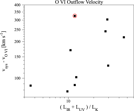
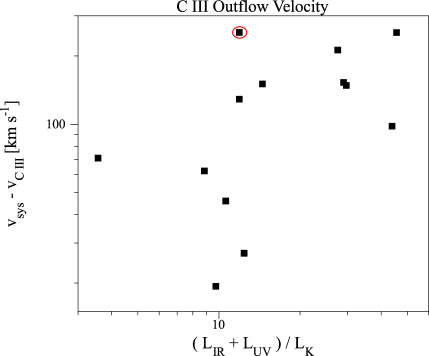
Figure 44: O VI  and C III  outflow velocities versus $\rm(L_{IR}+L_{UV})/L_{K}$. While these plots have a large degree of scatter, the higher SFR/Mass galaxies tend to have higher outflow velocities. NGC 3310 (which has unusually large outflow velocities for its mass and star formation rate) is denoted by a red circle.

Since the outflow speeds increase with both SFR and stellar mass, it is instructive to examine the outflow speeds as a function of the specific SFR (SFR/$M_{*}$). To do this, we have plotted the median O VI  and C III outflow velocities versus $\rm(L_{IR}+L_{UV})/L_{K}$ in Figure 44. While these plots show a significant amount of scatter, we see that the outflow speeds generally increase with the specific SFR. The O VI outflow velocity correlates more strongly with $\rm(L_{IR}+L_{UV})/L_{K}$ than does the C III velocity. As previously discussed, the properties of O VI are closely tied to the wind and thus presumably to the SFR.

The case of NGC 3310 requires further discussion as it is a significant outlier in most of our plots, with an outflow speed that is larger than expected for its SFR or mass. We note that the very large outflow speeds we see have been confirmed with STIS far-UV spectra of three individual regions in NGC 3310 (Schwartz et al. 2006). Examining the UV morphology of NGC 3310 in Figure 2, we see that NGC 3310 is the only galaxy with significant star formation spread throughout multiple locations in the FUSE  aperture. Radio HI velocity maps (Kregel & Sancisi, 2001) of the regions observed by FUSE  display a spread of almost 200 $\rm{km\,s^{-1}}$  which could increase the observed width of our absorption features, but should not produce highly blueshifted absorption. Another way in which NGC 3310 stands out within our sample is that it is the highest metallicity galaxy with $\rm\log(O/H)+12=9.0$. In principle, higher metallicity could allow us to probe gas with lower total column density. However, as we will show below the strengths of the strong absorption lines do not depend significantly on metallicty in our sample. Thus, this is unlikely to explain the large observed outflow speed in NGC 3310.

NGC 3310 is included in the young stellar population study of 16 starburst galaxies (11 also in our sample) by Pellerin & Robert (2007). By fitting the FUV spectra with models of instantaneous bursts, they estimated an age of $18\pm 2$ Myr for the starburst in NGC 3310 which was 10 Myrs older than any of the other galaxies in their sample. As the Type II supernovae that drive the galactic wind persist for 40 Myr, the total amount of kinetic energy injected into the wind will increase as the starburst ages. NGC 3310 appears to be a more mature starburst and may therefore have a more evolved wind.

3.4 Absorption-Line Equivalent Widths

It has known for some time that the strengths of the UV interstellar absorption-lines correlate with other key properties of starbursts. Heckman et al. (1998) used IUE spectra of 45 local starbursts to show that the equivalent widths of the strongest lines arising in the HI phase of the ISM correlated postively with the amount of UV extinction and reddening, the galaxy rotation speed and absolute magnitude, the metallicity, and SFR. Unfortunately, the poor spectral resolution and modest S/N of these spectra did not allow them to determine the astrophysics underlying these correlations. Because starbursts in more massive galaxies are known to have higher metallicity (Tremonti et al., 2004), higher SFR, and higher extinction (Heckman et al., 1998) it is especially difficult to sort out the fundamental relations from secondary correlations.

In general, the equivalent width of an interstellar absorption-line will depend on very different parameters depending on the optical depth of the line. In the limiting case of optically-thick gas the equivalent width is set purely by the product of velocity width of the line (the Doppler b-parameter) and the fraction of the UV continuum source covered by the absorber (the covering factor). In the case of optically thin gas the equivalent width is determined by the product of the ionic column density, the oscillator strength of the transition, and the covering factor. In our data we have examples of both optically thick and optically-thin transitions. Because the optically-thick lines are black (or nearly so) at line center, we know the covering factor is near unity.

We also probe gas spanning a range in ionization potential. We have described the properties of the coronal gas traced by O VI at some length, so here we will confine our attention to the lines tracing the HI phase (ionization potentials less than a Rydberg) and the HII phase (ionization potentials between 1 and 4 Rydbergs). For each of these two phase we will use one optically-thick and one optically-thin line. Hence, in Figure 45 we plot the equivalent widths of O I$\lambda 1039$, C II$\lambda 1036$, S III$\lambda 1012$, and C III$\lambda 977$  versus gas phase metallicity, K-band luminosity, and IR+UV luminosity. The first two lines trace the HI phase, with the O I  line being optically-thin and C II  optically-thick. The second two lines trace the HII phase, with the S III  line being optically-thin and C III  optically-thick.

In fact, the only pattern that emerges is that the poorest correlations are those between the equivalent widths of the lines tracing the HII phase (the C III  and sthw  lines) and the metallicity (Kendall $\tau_{a}=0.38$ and 0.44 respectively). All the other correlations are of comparable strength (Kendall $\tau_{a}=0.56$ to 0.75). This may reflect the relatively small sample size and the fact that the different starburst propertiues are interconnected: galaxies with higher masses will have higher velocity dispersions, higher SFRs, and higher metallicity.

3.5 Lyman Continuum Emission

One of the major puzzles in cosmology today is determining the source of the UV photons required to reionize the universe at redshifts $\rm{6\lesssim z\lesssim 14}$ (Fan et al., 2006). The known population of AGN do not appear to be sufficient by a wide margin, and the leading candidates are star forming galaxies (Stiavelli et al., 2004; Panagia et al., 2005). While stars in the early universe are thought be able to produce enough UV photons, it is not well understood what fraction of these photons can escape through the neutral hydrogen gas of the host galaxy (Yan & Windhorst, 2004) into the IGM. Superwinds, driven by starbursts, may be able to enhance the fraction of ionizing radiation by clearing channels through the surrounding gas (Dove et al., 2000).

The escape of ionizing continuum radiation from star forming galaxies was first observed by Steidel et al. (2001) in a sample of $\rm{z\sim 3.4}$ LBGs. More recent work by Shapley et al. (2006) focused on deep rest-frame UV spectroscopy and found a sample-averaged relative Lyman continuum escape fraction ($f_{esc}$) of 14%. They however detected Lyman continuum emission in only 2 of the 14 galaxies in their sample, which suggests that even at high redshifts ($\rm{z\sim 3}$) ionizing radiation is either relatively rare or viewing angle dependent.

Determining the escape fraction in starburst galaxies is therefore an important step in evaluating the importance of starburst galaxies in reionizing the universe. Local searches for Lyman continuum emission have so far been inconclusive. Leitherer et al. (1995) and Hurwitz et al. (1997) found $f_{esc}\lesssim\,10\%$ in a galaxy sample based on HUT observationsi and Deharveng et al. (2001) obtained a similar result for Mrk 54 using FUSE. Most recently Bergvall et al. (2006) published an analysis showing the detection of Lyman continuum emission in Haro 11. We however re-analyzed the same data in Grimes et al. (2007) and did not find any convincing evidence of Lyman leakage. We showed that uncertainties in the background subtraction and geocoronal contamination were larger than any detected signal. We therefore placed a limit on the escaping Lyman continuum emission in Haro 11  of $f_{esc}\lesssim\,2\%$.

3.5.1 Below the Lyman Limit in Other Starbursts

We have looked directly for Lyman continuum emission in other galaxies observed by FUSE. In order to move the Lyman limit farther from the detector edge, we have chosen the nine highest redshift galaxies in our sample. Figures 46 and 47 show the SiC 2A spectra for the nine galaxies plotted in order of increasing redshift. While the SiC 1B spectra also cover this wavelength regime, background subtraction problems are even more severe for the SiC 1B channel. In order to minimize contamination by dayglow we have plotted the night only spectra for all of the galaxies with the exception of VV 114. In the case of VV 114, there was not enough night time exposure to exclude the day observations.

We have plotted the spectra in the observed frame so that airglow features may be more easily identified. The intrinsic Lyman continuum region for each galaxy is also clearly marked. Several of the spectra are very noisy and systematic flux offsets caused by background over-subtraction in the CALFUSE pipeline are observed. As would be expected, the background subtraction problems are much more prevalent in the lower S/N spectra , specifically SBS 0335-052, Tol 0440-381, IRAS 19245-4140, and NGC 7673. A large number of apparent emission features can be observed, particularly in the wavelength region between 920-930 Å. These are easily observed in the day/night spectrum of VV 114  but also in the night only spectra of Tol 0440-381. These features, while varying widely in relative strength, are found at the same wavelengths in most of the spectra. They are properly identified as geocoronal emission features, mostly H I, O I, N I, and $\rm{N_{2}}$. For comparison, LWRS spectra (SiC 1B) of airglow and the earth limb are found in Figure 48. The large number of variable emission features highlights the difficulty in studying Lyman continuum emission in this wavelength regime.

No convincing evidence of Lyman continuum emission is seen in any of the nine spectra. All of the galaxies have flat spectra in the Lyman continuum regions with continuum levels at or below zero. The spectra with continuum levels below zero are indicative of background over-subtraction by the CALFUSE pipeline. This is commonly observed in low S/N FUSE  spectra on the SiC 1B and SiC 2A detectors as discussed previously, and highlights the difficulty in studying Lyman continuum emission. The FUSE  background dominates the signal in these wavelength regions. The emission features that are observed can all be identified as geo-coronal emission, with varying strengths in all of the spectra. In addition to these extracted spectra, we have also examined the 2-D detector images. A visual inspection of the 2-D spectra confirm our analysis of the one-dimensional spectra as we do not observe any evidence of Lyman continuum emission.

We have chosen to derive numerical limits for the five galaxies with S/N$>$5 on the LiF 1A channel. We have excluded the lower S/N galaxies such as Tol 0440-381 and IRAS 19245-4140  due to the significant errors introduced by the background subtraction. IRAS 19245-4140  for example, has a S/N of only 1.3 longward of the Lyman limit on the SiC 2A channel. While these errors exist even in the five galaxies with higher S/N, we can still place meaningful limits on the Lyman escape fraction.

We follow the work of Shapley et al. (2006) in estimating both the absolute and relative escape fractions. The absolute escape fraction describes the fraction of ionizing photons that escape the host galaxy. The relative escape fraction neglects the effects of dust extinction and is defined as the percentage of escaping ionizing photons relative to escaping non-ionizing FUV photons (1500 Å, Shapley et al., 2006). The relative escape fraction was introduced due to the difficulty in determining the intrinsic ionizing flux for high-z galaxies.

For these five galaxies we have measured an upper limit to the flux below the Lyman limit in each galaxy. We have then converted these to luminosities with $\rm L_{esc}\sim\lambda F_{\lambda}$ ($\lambda$=900 Å). From Starburst99 v5.1 (Vázquez & Leitherer, 2005) we find an intrinsic ratio of the bolometric to ionizing radiation of $\rm L_{bol}/L_{ioniz}\sim 7$. If we assume that the IR + UV luminosities dominate the bolometric luminosity as expected in these star-forming galaxies we derive:

$$\rm f_{esc,abs}=\frac{L_{esc}}{L_{UV}+L_{IR}}\left(\frac{L_{bol}}{L_{ioniz}}\right)_{intrinsic}.$$ (3)

We slightly modify $\rm f_{esc,rel}$ of Shapley et al. (2006) to use 1150 Å  instead of 1500 Å  as our reference wavelength. These values should be roughly comparable as we would expect the intrinsic luminosities of starburst galaxies to be comparable at 1150 Å  and 1500 Å  (Leitherer et al., 2002). We estimate $\rm f_{esc,rel}$ from

$$\rm f_{esc,rel}=\left(\frac{L_{900\,\AA}}{L_{1150\,\AA}}\right)_{obs}\left(\frac{L_{1150\,\AA}}{L_{900\,\AA}}\right)_{intrinsic}.$$ (4)

We obtain an intrinsic ratio $\rm L_{1150\,\AA}/L_{900\,\AA}\sim 4$ from Starburst99. The derived values for $\rm f_{esc,rel}$ and $\rm f_{esc,abs}$ are found in Table 23. The observed fluxes and luminosities have been corrected for MW extinction using Cardelli et al. (1989). We find $\rm f_{esc,abs}<0.2-7\%$ and $\rm f_{esc,rel}<9-26\%$ for the galaxies. The weakest limit, $\rm f_{esc,rel}<26\%$, is from VV 114  which is known to contain strong intrinsic dust attenuation (Goldader et al., 2002). Our upper limits for $\rm f_{esc,rel}$ are comparable to the average value of 14 LBGs with $\rm<f_{esc,rel}>\sim 14\%$ from Shapley et al. (2006). This average value in the high redshift sample however is dominated by two galaxies with $\rm f_{esc,rel}>40\%$. While our low redshift limits are compatible with the sample averaged values of $\rm f_{esc,rel}$ in LBGs, our limits show that the extreme Lyman continuum leakage observed in some LBGs is not observed in our small, local sample.

3.5.2 Limits from C II

Given the difficulties in directly observing Lyman continuum emission on the SiC detectors it is useful to investigate the Lyman escape fraction using a different method. Previously, Heckman et al. (2001b) have argued that since the optical depth at the Lyman edge must be much larger than that of the optical depth at line center for C II, we can then use the residual intensity in the core of the C II  line to place upper limits on the escape fraction at the Lyman limit.

Assuming that C II  is the dominant ionic species of carbon in the H I phase, Heckman et al. (2001b) derive

$$\tau_{\rm Ly}=4\times 10^{-16}\,(N_{H}/N_{j})\,(b/f\lambda)\,\tau_{\rm C}=8.6\,Z_{\rm C}^{-1}\,(b/100\,{\rm{km\,s^{-1}}})\,\tau_{\rm C}$$ (5)

where $\rm Z_{C}$ is the gas-phase carbon abundance in solar units and $b$ is the Doppler parameter. In our earlier gaussian fits to C II, we find that $b$ varies from $\sim 65-470\,{\rm{km\,s^{-1}}}$. Using the smallest Doppler parameter and solar abundances we expect the optical depth at the Lyman edge would be a factor of $\sim 5$ times larger than the C II  optical depth. As the majority of the galaxies in our sample have broader lines and sub-solar abundances, we would expect the Lyman limit optical depth to be enhanced by an even greater value.

An examination of the C II  feature for the galaxies in our sample (e.g. Figures 20 - 35) shows that it is nearly black in almost all cases. Given our estimates of the optical depth enhancement expected at the Lyman limit, this suggests that none of the galaxies in our sample have significant amounts of escaping Lyman continuum emission.

The most likely scenario for the escape of Lyman continuum emission is the picket fence model. Instead of a uniform slab of hydrogen surrounding a galaxy, holes in the gas surrounding the galaxy would allow ionizing photons to escape into the IGM. Starburst driven outflows could, for example, create “tunnels” in the surrounding neutral gas. The picket fence model would explain the variability seen in the center of some of the C II  features. For example, in Figure 21 of VV 114’s C II  profile a small fraction of photons are escaping at 0 $\rm{km\,s^{-1}}$  while the line is completely black at both $\sim\pm 100\,{\rm{km\,s^{-1}}}$. The few galaxies with a significant C II  escape fraction stand out due to their low metallicity, suggesting that their Lyman continuum escape fraction would still be very low.

We have conservatively estimated the continuum level and calculated a residual relative intensity for the C II line center. We calculate an upper limit to $\rm f_{esc,CII}$ by finding the upper bound to the normalized residual flux near line center. Only our highest redshift galaxy Mrk 54 has been excluded, as the C II  feature falls in the gap between the LiF channels. We also estimate upper limits for Lyman continuum emission using $\rm f_{esc,abs}$$=\rm f_{esc,CII}\,L_{UV}/(L_{UV}+L_{IR})$ following the methods of the previous section. For all but one of the galaxies in our sample we find $\rm f_{esc,abs}$$\lesssim 2\%$.

Using Equation 5 we have also estimated the optical depth of the Lyman limit using our estimate of the C II escape fraction and assuming the slab model of hydrogen surrounding a galaxy. The Doppler parameters are found from our Gaussian fits in Tables 3 - 18. As many of these lines are non-gaussian these must be considered only rough estimates. We have used the gas phase oxygen metallicities in Table 1 for the carbon metallicity and solar oxygen abundances from Asplund et al. (2005). The results can be found in Table 24. Our lowest derived optical depth is $\rm\tau_{Ly}\sim 20$ found for NGC 3310 but the majority of galaxies have $\rm\tau_{Ly}\gtrsim 100$. While these optical depths are only rough estimates, they suggest that the Lyman limit optical depth is well above the threshold needed to allow Lyman photons to escape the galaxy in the case of the simple slab model.

4 Conclusions

Starburst driven outflows are a cosmologically important example of galactic feedback. These outflows drive gas, metals, and energy out of galaxy centers and possibly into the IGM. Outflows in the early universe may also blow out “tunnels” allowing Lyman continuum photons from stars to escape the galaxy and reionize the universe. Studies of these superwinds are therefore vital to expanding our understanding of galaxy formation and evolution.

The extreme scale and energetics of starburst driven outflows complicate studies of their properties. Originating as a hot (T $>10^{8}\,$K) wind fluid, the outflows expand out into ambient gas of the galaxy and possibly beyond. Shocks, other hydrodynamical interactions, and entrained ambient gas and dust produce a complicated, multiphase outflow that requires panchromatic observations to properly characterize it.

Observations in the FUV play an important role in understanding outflows as they probe the neutral, ionized, and coronal gas. This gas traces the interaction between the hot outflowing wind fluid and the denser ambient ISM. Unfortunately, due to observational constraints at both low redshifts (due to UV atmospheric absorption) and high redshifts (due to contamination by the Ly$\alpha$ forest), studies at these wavelengths were severely limited until the launch of the FUSE satellite in 1999. As the number of star-forming galaxies observed by FUSE  has grown, it now possible to study the global properties of these outflows in the FUV.

In this work we have analyzed FUV spectra of a sample of 16 local, star-forming galaxies covering almost three orders of magnitude in SFR and over two orders of magnitude in stellar mass. Interstellar medium absorption and stellar photospheric features are observed throughout the sample of spectra. The strongest ISM absorption lines are generally blueshifted by $\sim$ 80 to 300 ${\rm{km\,s^{-1}}}$ relative to thge galaxy systemic velocity, implying that galactic outflows are the norm in starbursts.

Coronal gas is an important coolant for gas at temperatures T$\sim 10^{5.5}\,$K and is only directly observable in the FUV through observations of the O VI$\lambda\lambda 1032,1038$  doublet. O VI  emission is only detected in 1 of the 16 galaxies in our sample. This suggests that radiative cooling of the coronal gas is not dynamically significant in the wind and does not impede its outflow. In contrast, O VI  absorption is nearly ubiquitous in our sample and is found to trace systematically higher outflow speeds than the photoionized and neutral gas. We find a strong relationship between O VI column density and the width of the line that is consistent with the production of O VI  in a radiatively cooling gas flow passing through the coronal temperature regime. This is expected to occur at the interface between the outrushing hot wind seen in X-rays and the cool dense material in its path.

Previous studies (Vázquez et al., 2004; Schwartz & Martin, 2004; Grimes et al., 2006) have suggested that the observed outflow velocities in a galaxy increase with the ionization potential of the species observed. While this is clearly the case for the coronal phase gas, it is not the case for the neutral and photoionized material. Our new results show that the derived outflow velocities in thius gas in a given galaxy increase with line strength (equivalent width) and not ionization state. This could be explained if the observations of the stronger lines probe lower column density gas than the weaker absorption features. The lower column density gas extends to greater outflow velocities and is not readily observable in weaker absorption features. We conclude that the extensive studies of outflows in the local star forming galaxies using the Na I$\lambda\lambda 5890,5896$ doublet in the optical should be able to reliably measure the outflow velocities that would be seen in the strong FUV absorption-lines. This is because the Na I$\lambda\lambda 5890,5896$  line should be sufficiently strong to probe the low column density outflowing gas.

In agreement with previous UV (Schwartz et al., 2006) and optical (Martin, 2005; Rupke et al., 2005) studies we find that the outflow velocities of the strongest absorption lines increase with increasing SFR and increasing specific SFR (SFR/M_∗). We speculate that starbursts with higher SFR generate more wind momentum which can accelerate the absorbing material (clouds) entrained in the wind to higher outflow velocities. Our sample does not probe the regime of very high SFR (of-order $10^{2}$ M_⊙ per year) where the relationship appears to flatten (Martin, 2005).

We find that the equivalent width of the optically thin lines arising in the HI phase correlates most strongly with the gas-phase metallicity (as expected since the equivalent width should be proportional to the column density of the metal species). In contrast, the equivalent widths of the optically-thick lines in the HI and HII phase correlate better with the galaxy mass and the SFR. This is consistent with the fact that the equivalent width for these optically-thick lines is determined by the velocity dispersion in the ISM. More massive galaxies and galaxies undergoing elevated SFR will have higher velocity dispersions due to both gravity and the kinetic energy input from massive stars.

Lastly, we have looked for escaping Lyman continuum emission in our sample. We find no convincing evidence of escaping ionizing radiation in any of the observed galaxies. In a subsample of five of our galaxies with suitable redshifts and data quality we find that the upper limit to the absolute fraction of escaping Lyman continuum photons ranges from $\rm f_{esc,abs}$$<0.2-6.3\%$. Following Shapley et al. (2006) we also derive upper limits to the realtive escape fractioni (the ratio of the fraction of escaping Lyman continuum and non-ionizing FUV continuum). These range from $\rm f_{esc,rel}$$<9-26\%$ for this subsample. While our upper limits are compatible with observations of high redshift Lyman Break Galaxies, we do not observe any evidence of Lyman continuum emission as observed in some Lyman Break Galaxies.

Using the escape fraction of light at the center of the C II  feature we also place limits on the escape fraction of Lyman continuum emission in 15 of the galaxies included in our sample. In a simple model where a galaxy is surrounded by a slab of neutral hydrogen we find significant optical depths at the Lyman limit of $\tau_{\rm Ly}>20$. In a more realistic model with holes in the neutral gas surrounding a galaxy, we find $\rm f_{esc,abs}$$<2\%$ for almost all of the galaxies. This suggests that local starburst galaxies are not allowing the escape of significant amounts of hydrogen ionizing photons, even in galaxies with strong winds.

This work provides a unique view of the properties of outflows in star-forming galaxies. The wealth of absorption features over a variety of gas phases enables direct comparisons difficult in other wavelength regimes. The projected physical size of FUSE’s large spectroscopic aperture for these local starbursts is particularly well matched to high redshift spectrographic observations of Lyman Break Galaxies and other star forming galaxies - both probe the outflows on the galactic scale. Thus, this study should provide an excellent complement to the high redshift observations.

Table 1: FUSE Galaxy Properties

Galaxy	$\rm{v_{sys}}$	Distance	MW E(B-V)	$\rm{L_{FUV}}$	$\rm{L_{K}}$	$\rm{L_{IR}}$	$\rm{L_{UV}+L_{IR}}$	$\rm{F_{60\mu m}/F_{100\mu m}}$	Z
	($\rm{km\,s^{-1}}$)	(Mpc)	(mag)	$\rm{(L_{\odot})}$	$\rm{(L_{\odot})}$	$\rm{(L_{\odot})}$	$\rm{(L_{\odot})}$		(log[O/H]+12)
HARO11	6175	88	0.011	$1.6\times 10^{10}$	$4.5\times 10^{9}$	$1.9\times 10^{11}$	$2.1\times 10^{11}$	1.37	7.9
VV114	6016	86	0.016	$2.4\times 10^{10}$	$2.0\times 10^{10}$	$5.2\times 10^{11}$	$5.4\times 10^{11}$	0.73	8.6
NGC1140	1501	21	0.038	$2.4\times 10^{9}$	$7.7\times 10^{8}$	$4.4\times 10^{9}$	$6.8\times 10^{9}$	0.68	8.0
SBS0335-052	4043	57	0.047	$2.6\times 10^{9}$	$\cdots$	$\cdots$	$\cdots$	$\cdots$	7.3
TOL0440-381	12291	178	0.015	$1.7\times 10^{10}$	$2.8\times 10^{9}$	$2.4\times 10^{10}$	$4.1\times 10^{10}$	$\cdots$	8.2
NGC1705	632	8	0.008	$1.0\times 10^{9}$	$1.3\times 10^{8}$	$2.6\times 10^{8}$	$1.3\times 10^{9}$	0.38	8.0
NGC1741	4037	57	0.051	$1.1\times 10^{10}$	$1.6\times 10^{9}$	$3.8\times 10^{10}$	$4.9\times 10^{10}$	0.71	8.0
IZW18	751	10	0.032	$1.3\times 10^{8}$	$\cdots$	$\cdots$	$\cdots$	$\cdots$	7.2
NGC3310	983	14	0.022	$2.4\times 10^{9}$	$1.9\times 10^{9}$	$2.0\times 10^{10}$	$2.3\times 10^{10}$	0.78	9.0
HARO3	963	13	0.007	$4.2\times 10^{8}$	$2.7\times 10^{8}$	$3.0\times 10^{9}$	$3.4\times 10^{9}$	0.82	8.3
NGC3690	3121	44	0.017	$6.3\times 10^{9}$	$2.3\times 10^{10}$	$6.6\times 10^{11}$	$6.7\times 10^{11}$	0.93	8.8
NGC4214	291	4	0.022	$2.1\times 10^{8}$	$3.1\times 10^{8}$	$9.0\times 10^{8}$	$1.1\times 10^{9}$	0.60	8.2
MRK54	13450	196	0.015	$5.2\times 10^{10}$	$7.7\times 10^{9}$	$1.2\times 10^{11}$	$1.7\times 10^{11}$	0.51	8.6
IRAS19245-4140	2832	40	0.087	$8.8\times 10^{9}$	$3.9\times 10^{8}$	$8.2\times 10^{9}$	$1.7\times 10^{10}$	1.67	8.0
NGC7673	3392	48	0.043	$6.7\times 10^{9}$	$3.2\times 10^{9}$	$3.2\times 10^{10}$	$3.9\times 10^{10}$	0.74	8.5
NGC7714	2803	39	0.052	$9.4\times 10^{8}$	$5.3\times 10^{9}$	$5.6\times 10^{10}$	$5.7\times 10^{10}$	0.91	8.7

Note. — $\rm{v_{sys}}$, MW E(B-V), IRAS, and K-Band fluxes were obtained from NED where available. IRAS (Soifer, Boehmer, Neugebauer, & Sanders, 1989; Moshir et al., 1993) and 2Mass (Jarrett et al., 2003) luminosities are transformed using methods of Sanders & Mirabel (1996) and Carpenter (2001) respectively. The references for the gas-phase nebular metallicity measurements are as follows, Haro 11  (Bergvall & $\rm{\ddot{O}}$stlin, 2002), VV 114 (Kim et al., 1995; Charlot & Longhetti, 2001), NGC 1140, NGC 1705, NGC 3310, NGC 3690, NGC 4214, NGC 7673, NGC 7714 (Heckman et al., 1998), SBS 0335-052 (Izotov et al., 1997), Tol 0440-381 (Terlevich et al., 1991; Pellerin & Robert, 2007), NGC 1741 (Conti et al., 1996), Haro 3 (Izotov & Thuan, 2004), I Zw 18 (Izotov & Thuan, 1999), IRAS 19245-4140 (Östlin et al., 2007), and Mrk 54 (spectrum from A. Boselli with conversions from Charlot & Longhetti, 2001).

Table 2: FUSE Observation Data

Galaxy	FUSE  Pointing		Aperture	Region	DAY/NIGHT	Obs. Date	PI	Obs. Time	Exposures	S/N
	(J2000)					(UT)		(ks)
HARO 11	$00^{\rm h}36^{\rm m}52\fs 5$	$-33\arcdeg 33\arcmin 19\arcsec$	LWRS	PC	NIGHT	2001-10-12	Bergvall	11.9	6	7.2
VV 114	$01^{\rm h}07^{\rm m}46\fs 6$	$-17\arcdeg 30\arcmin 24\arcsec$	LWRS	PC	BOTH	2003-07-26	Heckman	11.2	4	6.6
NGC 1140	$02^{\rm h}54^{\rm m}33\fs 6$	$-10\arcdeg 01\arcmin 39\arcsec$	LWRS	PC	BOTH	2001-11-28	Buat	3.9	2	4.8
SBS 0335-052	$03^{\rm h}37^{\rm m}43\fs 1$	$-05\arcdeg 02\arcmin 39\arcsec$	LWRS	PC	BOTH	2001-09-26	Thuan	24.4	8	4.1
TOL 0440-381	$04^{\rm h}42^{\rm m}08\fs 0$	$-38\arcdeg 01\arcmin 10\arcsec$	LWRS	PC	BOTH	2000-12-13	Deharveng	31.2	11	4.0
NGC 1705	$04^{\rm h}54^{\rm m}13\fs 5$	$-53\arcdeg 21\arcmin 39\arcsec$	LWRS	EC	BOTH	2000-02-04	Heckman	24.0	13	27.2
NGC 1741	$05^{\rm h}01^{\rm m}37\fs 7$	$-04\arcdeg 15\arcmin 30\arcsec$	LWRS	PC	NIGHT	2003-12-23	Heckman	18.5	10	8.4
IZW 18	$09^{\rm h}34^{\rm m}02\fs 3$	$+55\arcdeg 14\arcmin 25\arcsec$	LWRS	PC	BOTH	2001-02-11	Moos	58.2	37	9.7
NGC 3310	$10^{\rm h}38^{\rm m}45\fs 7$	$+53\arcdeg 30\arcmin 06\arcsec$	LWRS	EC	BOTH	2000-05-05	Heckman	27.1	11	18.0
HARO 3	$10^{\rm h}45^{\rm m}22\fs 4$	$+55\arcdeg 57\arcmin 37\arcsec$	LWRS	PC	NIGHT	2002-04-07	Thuan	4.9	4	6.2
NGC 3690	$11^{\rm h}28^{\rm m}31\fs 0$	$+58\arcdeg 33\arcmin 41\arcsec$	LWRS	PC	NIGHT	2001-03-25	Heckman	34.9	20	10.8
NGC 4214	$12^{\rm h}15^{\rm m}39\fs 4$	$+36\arcdeg 19\arcmin 35\arcsec$	LWRS	EC	BOTH	2000-05-12	Heckman	11.1	6	14.6
MRK 54	$12^{\rm h}56^{\rm m}55\fs 9$	$+32\arcdeg 26\arcmin 52\arcsec$	LWRS	PC	BOTH	2000-02-19	Deharveng	25.8	13	5.8
IRAS 19245-4140	$19^{\rm h}27^{\rm m}58\fs 0$	$-41\arcdeg 34\arcmin 27\arcsec$	LWRS	PC	NIGHT	2000-05-21	Buat	2.9	6	4.7
NGC 7673	$23^{\rm h}27^{\rm m}41\fs 6$	$+23\arcdeg 35\arcmin 30\arcsec$	LWRS	PC	NIGHT	2000-07-20	Buat	6.3	3	4.7
NGC 7714	$23^{\rm h}36^{\rm m}14\fs 1$	$+02\arcdeg 09\arcmin 19\arcsec$	MDRS	PC	BOTH	2001-12-04	Benjamin	78.4	46	4.3

Table 3: HARO11 ISM Absorption Line Fit Data

Ion	$\lambda_{0}$	$log(\lambda fN/N_{H})$	Instrument	$\rm{W}_{\lambda}$	$\rm{v_{c}}$	FWHM
	Å			Å	$\rm{km\,s^{-1}}$	$\rm{km\,s^{-1}}$
C III	977.02	-0.61	2asic	1.83$\pm$0.57	5998$\pm$6	269$\pm$10
O VI	1031.93	-1.13	1alif	0.38$\pm$0.06	6039$\pm$16	193$\pm$34
			2blif	0.39$\pm$0.07	6050$\pm$14	159$\pm$34
C II	1036.34	-1.37	1alif	1.29$\pm$0.05	6063$\pm$6	381$\pm$18
			2blif	1.24$\pm$0.13	6074$\pm$8	344$\pm$36
O I	988.73	-1.56	1alif	0.72$\pm$0.05	6092$\pm$14	276$\pm$14
			2blif	0.66$\pm$0.09	6079$\pm$23	304$\pm$26
N II	1083.99	-2.00	1blif	0.92$\pm$0.07	6081$\pm$10	353$\pm$28
			2alif	1.00$\pm$0.08	6085$\pm$11	381$\pm$33
N III	989.80	-2.03	1alif	1.04$\pm$0.05	6076$\pm$6	276
			2blif	1.05$\pm$0.08	6073$\pm$10	304
O I	1039.23	-2.29	1alif	0.35$\pm$0.07	6112$\pm$14	244$\pm$51
			2blif	0.37$\pm$0.12	6130$\pm$16	200$\pm$77
N I	1134.41	-2.57	2alif	0.15	6048$\pm$79	300
Fe II	1096.88	-2.96	2alif	0.20$\pm$0.04	6119$\pm$9	131$\pm$24
Si II	1020.70	-2.99	1alif	0.53$\pm$0.18	6023$\pm$17	339$\pm$88
			2blif	0.32$\pm$0.10	6015$\pm$17	232$\pm$67
Fe II	1121.97	-3.14	2alif	0.25	6088$\pm$68	203
S III	1012.50	-3.24	1alif	0.52$\pm$0.18	6083$\pm$6	225
			2blif	0.68$\pm$0.22	6078$\pm$13	290$\pm$75
Fe II	1125.45	-3.41	2alif	0.23$\pm$0.05	6062$\pm$17	195$\pm$37
Ar I	1066.66	-3.58	2alif	0.54$\pm$0.08	6136$\pm$20	332$\pm$55
	1128.00	-4.01	2alif	0.14	6202$\pm$74	327
P V s	1117.98		2alif	0.30$\pm$0.06	6165$\pm$24	327$\pm$63
Si IV s	1122.48		2alif	0.63$\pm$0.09	6163$\pm$17	222$\pm$29
Si IV s	1128.33		2alif	0.30	6202	327

Table 4: HARO3 ISM Absorption Line Fit Data

Ion	$\lambda_{0}$	$log(\lambda fN/N_{H})$	Instrument	$\rm{W}_{\lambda}$	$\rm{v_{c}}$	FWHM
	Å			Å	$\rm{km\,s^{-1}}$	$\rm{km\,s^{-1}}$
C III	977.02	-0.61	2asic	1.16	913$\pm$26	202$\pm$16
O VI	1031.93	-1.13	1alif	0.71$\pm$0.08	787$\pm$26	324
			2blif	0.85$\pm$0.12	796$\pm$21	324$\pm$53
C II	1036.34	-1.37	1alif	0.97$\pm$0.07	868$\pm$3	229$\pm$26
			2blif	1.11$\pm$0.13	876$\pm$10	259$\pm$54
O I	988.73	-1.56	1alif	0.97	912$\pm$11	150
			2blif	0.46$\pm$0.06	906$\pm$4	88$\pm$14
N III	989.80	-2.03	1alif	0.87	914$\pm$6	127$\pm$2
			2blif	0.59	920$\pm$22	110
O I	1039.23	-2.29	1alif	0.51$\pm$0.04	895$\pm$4	120$\pm$16
			2blif	0.47$\pm$0.10	905$\pm$2	86$\pm$5
N I	1134.98	-2.39	1blif	0.33$\pm$0.04	900$\pm$8	118
			2alif	0.30$\pm$0.04	901$\pm$12	144
Fe II	1144.94	-2.42	1blif	0.42$\pm$0.07	891$\pm$5	85$\pm$22
			2alif	0.45$\pm$0.10	871$\pm$12	172$\pm$44
N I	1134.41	-2.57	1blif	0.41$\pm$0.04	884$\pm$6	118$\pm$11
			2alif	0.38$\pm$0.04	878$\pm$8	144$\pm$14
Fe II	1096.88	-2.96	1blif	0.34$\pm$0.06	904$\pm$8	117$\pm$20
			2alif	0.31$\pm$0.06	886$\pm$9	139$\pm$24
Si II	1020.70	-2.99	1alif	0.35$\pm$0.04	912$\pm$4	107$\pm$15
			2blif	0.41$\pm$0.13	941$\pm$15	118$\pm$37
Fe II	1121.97	-3.14	1blif	0.43$\pm$0.08	902$\pm$9	132$\pm$29
			2alif	0.46$\pm$0.12	924$\pm$16	156$\pm$42
Fe II	1143.23	-3.19	1blif	0.21$\pm$0.08	894$\pm$12	86
			2alif	0.25$\pm$0.07	907$\pm$13	134$\pm$36
S III	1012.50	-3.24	1alif	0.40$\pm$0.07	921$\pm$8	130$\pm$22
			2blif	0.45$\pm$0.06	920$\pm$6	109$\pm$18
Ar I	1066.66	-3.58	1alif	0.14	888$\pm$31	80
			2blif	0.19$\pm$0.07	897$\pm$10	67
Si IV s	1122.48		1blif	0.47$\pm$0.08	922$\pm$7	129$\pm$26
			2alif	0.44$\pm$0.06	902$\pm$4	105$\pm$15
C III s	1175.59		1blif	1.50$\pm$0.15	938$\pm$31	500

Table 5: IRAS19245-4140 ISM Absorption Line Fit Data

Ion	$\lambda_{0}$	$log(\lambda fN/N_{H})$	Instrument	$\rm{W}_{\lambda}$	$\rm{v_{c}}$	FWHM
	Å			Å	$\rm{km\,s^{-1}}$	$\rm{km\,s^{-1}}$
C III	977.02	-0.61	2asic	2.50$\pm$0.74	2748$\pm$29	663$\pm$235
C II	1036.34	-1.37	1alif	0.86$\pm$0.09	2746$\pm$11	272$\pm$30
			2blif	0.75$\pm$0.25	2761$\pm$31	256$\pm$96
O I	988.73	-1.56	1alif	0.31$\pm$0.03	2774$\pm$8	81$\pm$13
N II	1083.99	-2.00	2alif	0.17	2792$\pm$14	72
N III	989.80	-2.03	1alif	0.32	2708$\pm$7	89
N I	1134.41	-2.57	1blif	0.38	2782$\pm$1	50$\pm$11
			2alif	0.30	2794$\pm$0	37
Si II	1020.70	-2.99	1alif	0.14$\pm$0.05	2821$\pm$9	59$\pm$21
			2blif	0.07	2820$\pm$27	59
Ar I	1048.22	-3.00	1alif	0.08	2787$\pm$14	48
Fe II	1121.97	-3.14	1blif	0.11	2862$\pm$15	67
			2alif	0.14	2828$\pm$11	45
S III	1012.50	-3.24	1alif	0.32	2785$\pm$5	50$\pm$7
			2blif	0.30	2793$\pm$8	50
Si IV s	1122.48		1blif	0.18$\pm$0.02	2830$\pm$6	60$\pm$12
			2alif	0.21	2829$\pm$11	60
C III s	1175.59		1blif	2.55$\pm$0.50	2795$\pm$25	641$\pm$130

Table 6: IZW18 ISM Absorption Line Fit Data

Ion	$\lambda_{0}$	$log(\lambda fN/N_{H})$	Instrument	$\rm{W}_{\lambda}$	$\rm{v_{c}}$	FWHM
	Å			Å	$\rm{km\,s^{-1}}$	$\rm{km\,s^{-1}}$
C II	1036.34	-1.37	1alif	0.63$\pm$0.05	748$\pm$7	180$\pm$16
			2blif	0.65$\pm$0.06	757$\pm$8	190$\pm$18
O I	988.73	-1.56	1alif	0.64$\pm$0.23	784$\pm$4	106$\pm$12
			2asic	0.54	816$\pm$5	84$\pm$15
N III	989.80	-2.03	1alif	0.51$\pm$0.10	711$\pm$9	122$\pm$28
			2asic	0.69$\pm$0.15	754$\pm$11	180$\pm$68
O I	1039.23	-2.29	1alif	0.18$\pm$0.02	759$\pm$5	76$\pm$9
			2blif	0.23$\pm$0.03	770$\pm$5	79$\pm$13
Si II	1020.70	-2.99	1alif	0.15$\pm$0.02	774$\pm$8	100
			2blif	0.17$\pm$0.03	788$\pm$11	100
Fe II	1121.97	-3.14	1blif	0.10$\pm$0.03	751$\pm$8	65$\pm$22
			2alif	0.13$\pm$0.01	769$\pm$2	57$\pm$6
Fe II	1125.45	-3.41	1blif	0.09$\pm$0.02	745$\pm$6	56$\pm$16
			2alif	0.11$\pm$0.02	772$\pm$6	79$\pm$15
Ar I	1066.66	-3.58	1alif	0.06	758$\pm$20	70
Si IV s	1122.48		1blif	0.18$\pm$0.05	753$\pm$17	149$\pm$54
			2alif	0.21$\pm$0.02	768$\pm$5	126$\pm$15
Si IV s	1128.33		1blif	0.18	775$\pm$34	155
			2alif	0.18	779$\pm$68	228
C III s	1175.59		1blif	0.86$\pm$0.07	747$\pm$15	423$\pm$38
			2alif	0.81$\pm$0.06	757$\pm$12	388$\pm$30

Table 7: MRK54 ISM Absorption Line Fit Data

Ion	$\lambda_{0}$	$log(\lambda fN/N_{H})$	Instrument	$\rm{W}_{\lambda}$	$\rm{v_{c}}$	FWHM
	Å			Å	$\rm{km\,s^{-1}}$	$\rm{km\,s^{-1}}$
C III	977.02	-0.61	1alif	1.76$\pm$0.12	13382$\pm$12	434$\pm$46
			2blif	1.48$\pm$0.09	13402$\pm$6	368$\pm$28
O VI	1031.93	-1.13	1alif	0.77$\pm$0.09	13321$\pm$14	287$\pm$38
O I	988.73	-1.56	1alif	1.18$\pm$0.34	13541$\pm$46	386$\pm$112
			2blif	0.82$\pm$0.19	13526$\pm$30	337$\pm$86
N II	1083.99	-2.00	1blif	1.41$\pm$0.12	13466$\pm$9	409$\pm$39
			2alif	1.60$\pm$0.13	13469$\pm$10	497$\pm$44
N III	989.80	-2.03	1alif	0.67$\pm$0.11	13481$\pm$13	177$\pm$45
			2blif	0.82	13463$\pm$5	138$\pm$20
Si II	1020.70	-2.99	1alif	0.53$\pm$0.15	13544$\pm$58	300
			2blif	0.81$\pm$0.07	13528$\pm$21	400
S III	1012.50	-3.24	1alif	0.62$\pm$0.11	13432$\pm$14	310$\pm$46
			2blif	0.54$\pm$0.12	13429$\pm$15	277$\pm$56
S IV s	1062.66		1blif	0.64$\pm$0.07	13529$\pm$27	400
			2alif	0.74$\pm$0.06	13525$\pm$20	400
Si IV s	1122.48		1blif	0.96$\pm$0.12	13434$\pm$14	312$\pm$44
			2alif	0.97$\pm$0.16	13423$\pm$24	334$\pm$62
Si IV s	1128.33		2alif	0.71$\pm$0.07	13453$\pm$14	299$\pm$33

Table 8: NGC1140 ISM Absorption Line Fit Data

Ion	$\lambda_{0}$	$log(\lambda fN/N_{H})$	Instrument	$\rm{W}_{\lambda}$	$\rm{v_{c}}$	FWHM
	Å			Å	$\rm{km\,s^{-1}}$	$\rm{km\,s^{-1}}$
C III	977.02	-0.61	2asic	1.32$\pm$0.18	1438$\pm$11	268$\pm$46
C II	1036.34	-1.37	1alif	0.93$\pm$0.08	1481$\pm$6	250$\pm$21
			2blif	1.33$\pm$0.27	1487$\pm$27	358$\pm$76
O I	988.73	-1.56	2asic	0.51$\pm$0.12	1542$\pm$5	100
			2blif	0.75	1548$\pm$6	100
N II	1083.99	-2.00	2alif	0.63$\pm$0.10	1517$\pm$7	177$\pm$28
N III	989.80	-2.03	2asic	0.99	1502$\pm$5	138$\pm$39
			2blif	0.69$\pm$0.10	1517$\pm$7	130
O I	1039.23	-2.29	1alif	0.45$\pm$0.03	1510$\pm$2	110$\pm$11
			2blif	0.42$\pm$0.05	1526$\pm$4	112$\pm$13
N I	1134.98	-2.39	1blif	0.24$\pm$0.05	1505$\pm$12	109$\pm$21
			2alif	0.22$\pm$0.03	1515$\pm$8	103
Fe II	1144.94	-2.42	1blif	0.39$\pm$0.04	1511$\pm$6	105
			2alif	0.39$\pm$0.06	1534$\pm$6	121$\pm$21
N I	1134.41	-2.57	1blif	0.30$\pm$0.04	1490$\pm$8	109$\pm$14
			2alif	0.26$\pm$0.03	1491$\pm$7	103$\pm$11
Fe II	1063.18	-2.70	1alif	0.37$\pm$0.06	1504$\pm$9	145$\pm$30
			2blif	0.44$\pm$0.09	1514$\pm$13	147$\pm$37
Fe II	1096.88	-2.96	1blif	0.26$\pm$0.05	1503$\pm$9	122$\pm$28
			2alif	0.27$\pm$0.04	1515$\pm$7	112$\pm$21
Ar I	1048.22	-3.00	1alif	0.16$\pm$0.04	1512$\pm$16	130
			2blif	0.26$\pm$0.05	1529$\pm$13	130
Fe II	1121.97	-3.14	1blif	0.31$\pm$0.10	1512$\pm$10	115$\pm$42
			2alif	0.32	1494$\pm$25	148
S III	1012.50	-3.24	1alif	0.47$\pm$0.09	1509$\pm$9	175$\pm$31
			2blif	0.50	1501$\pm$27	168
Ar I	1066.66	-3.58	1alif	0.16$\pm$0.04	1493$\pm$24	130
Si IV s	1122.48		1blif	0.41$\pm$0.08	1512$\pm$10	132$\pm$31
			2alif	0.67$\pm$0.18	1494$\pm$25	208$\pm$47
C III s	1175.59		1blif	1.16$\pm$0.07	1498$\pm$14	300

Table 9: NGC1705 ISM Absorption Line Fit Data

Ion	$\lambda_{0}$	$log(\lambda fN/N_{H})$	Instrument	$\rm{W}_{\lambda}$	$\rm{v_{c}}$	FWHM
	Å			Å	$\rm{km\,s^{-1}}$	$\rm{km\,s^{-1}}$
C III	977.02	-0.61	1bsic	1.21$\pm$0.29	613$\pm$20	310
			2asic	1.23	651$\pm$28	325
O VI	1031.93	-1.13	1alif	0.18$\pm$0.01	554$\pm$3	111$\pm$9
			2blif	0.20$\pm$0.01	559$\pm$3	125$\pm$9
C II	1036.34	-1.37	1alif	1.01	600$\pm$37	262
			2blif	1.02$\pm$0.26	597$\pm$24	270$\pm$84
O I	988.73	-1.56	1alif	0.58$\pm$0.04	600$\pm$3	162$\pm$21
			2blif	0.53$\pm$0.04	596$\pm$4	153$\pm$14
N II	1083.99	-2.00	1asic	0.49$\pm$0.06	626$\pm$4	160$\pm$18
N III	989.80	-2.03	1alif	0.60$\pm$0.05	597$\pm$2	130$\pm$13
			2blif	0.63$\pm$0.04	594$\pm$3	145$\pm$14
O I	1039.23	-2.29	1alif	0.22	606$\pm$31	72
			2blif	0.23	600$\pm$32	77
N I	1134.98	-2.39	1blif	0.07$\pm$0.01	592$\pm$6	73
			2alif	0.05$\pm$0.01	593$\pm$3	50
Fe II	1144.94	-2.42	1blif	0.24$\pm$0.02	610$\pm$2	87$\pm$7
			2alif	0.25$\pm$0.02	609$\pm$2	89$\pm$7
N I	1134.41	-2.57	1blif	0.07$\pm$0.01	614$\pm$9	73$\pm$9
			2alif	0.05$\pm$0.01	597$\pm$8	50$\pm$15
Fe II	1096.88	-2.96	1blif	0.14$\pm$0.01	607$\pm$3	88$\pm$7
			2alif	0.11$\pm$0.02	603$\pm$5	67$\pm$14
Si II	1020.70	-2.99	1alif	0.09$\pm$0.01	613$\pm$2	77$\pm$7
			2blif	0.09$\pm$0.01	599$\pm$3	80
Fe II	1121.97	-3.14	1blif	0.18	620$\pm$50	120
			2alif	0.12	603$\pm$7	108$\pm$43
S III	1012.50	-3.24	1alif	0.18$\pm$0.02	608$\pm$11	130
			2blif	0.17$\pm$0.03	603$\pm$14	130
Ar I	1066.66	-3.58	1alif	0.11$\pm$0.02	622$\pm$9	110
			2blif	0.12$\pm$0.01	592$\pm$6	110
Si IV s	1122.48		1blif	0.40	627$\pm$47	172
			2alif	0.48$\pm$0.00	618$\pm$4	200$\pm$4
C III s	1175.59		1blif	1.67$\pm$0.04	639$\pm$4	515$\pm$13
			2alif	1.65$\pm$0.04	634$\pm$4	507$\pm$12

Table 10: NGC1741 ISM Absorption Line Fit Data

Ion	$\lambda_{0}$	$log(\lambda fN/N_{H})$	Instrument	$\rm{W}_{\lambda}$	$\rm{v_{c}}$	FWHM
	Å			Å	$\rm{km\,s^{-1}}$	$\rm{km\,s^{-1}}$
C III	977.02	-0.61	2asic	1.08	4007$\pm$20	164$\pm$15
O VI	1031.93	-1.13	1alif	0.58$\pm$0.08	3833$\pm$32	400
			2blif	0.58$\pm$0.20	3921$\pm$92	400
C II	1036.34	-1.37	1alif	1.38$\pm$0.07	3985$\pm$4	300$\pm$28
			2blif	1.39$\pm$0.19	3986$\pm$4	270$\pm$29
O I	988.73	-1.56	1alif	1.16$\pm$0.25	4024$\pm$10	234$\pm$56
			2blif	0.98	4046$\pm$11	182$\pm$50
N II	1083.99	-2.00	1blif	0.93$\pm$0.19	3957$\pm$9	277$\pm$57
			2alif	0.91$\pm$0.05	3982$\pm$5	263$\pm$16
N III	989.80	-2.03	1alif	0.84$\pm$0.10	4004$\pm$12	223$\pm$31
			2blif	0.79$\pm$0.15	3981$\pm$18	206$\pm$37
O I	1039.23	-2.29	1alif	0.58$\pm$0.07	3981$\pm$7	222$\pm$25
			2blif	0.49$\pm$0.07	3977$\pm$11	190$\pm$28
N I	1134.98	-2.39	1blif	0.16$\pm$0.06	3962$\pm$11	82$\pm$24
			2alif	0.16$\pm$0.04	3944$\pm$16	141$\pm$40
Fe II	1144.94	-2.42	2alif	0.40$\pm$0.04	3992$\pm$13	200
N I	1134.41	-2.57	1blif	0.20$\pm$0.07	3937$\pm$9	82$\pm$31
			2alif	0.31$\pm$0.05	3928$\pm$15	141$\pm$23
Fe II	1096.88	-2.96	1blif	0.30$\pm$0.05	3953$\pm$13	181$\pm$37
			2alif	0.30$\pm$0.06	3964$\pm$13	200$\pm$46
Si II	1020.70	-2.99	1alif	0.45$\pm$0.08	3954$\pm$8	211$\pm$34
			2blif	0.42$\pm$0.08	3963$\pm$8	180$\pm$35
Fe II	1121.97	-3.14	1blif	0.45$\pm$0.14	3979$\pm$22	204$\pm$54
			2alif	0.34	3978$\pm$42	199$\pm$70
S IV s	1062.66		1alif	0.38$\pm$0.05	4017$\pm$23	200
Si IV s	1122.48		1blif	0.58$\pm$0.10	4001$\pm$13	194$\pm$29
			2alif	0.59$\pm$0.15	4003$\pm$23	218$\pm$39

Table 11: NGC3310 ISM Absorption Line Fit Data

Ion	$\lambda_{0}$	$log(\lambda fN/N_{H})$	Instrument	$\rm{W}_{\lambda}$	$\rm{v_{c}}$	FWHM
	Å			Å	$\rm{km\,s^{-1}}$	$\rm{km\,s^{-1}}$
C III	977.02	-0.61	1bsic	2.44$\pm$0.05	701$\pm$5	583$\pm$19
			2asic	2.10$\pm$0.61	705$\pm$19	450$\pm$169
O VI	1031.93	-1.13	1alif	1.67$\pm$0.04	616$\pm$5	556$\pm$15
			2blif	1.71$\pm$0.04	620$\pm$5	554$\pm$15
C II	1036.34	-1.37	1alif	3.31$\pm$0.07	749$\pm$6	786$\pm$31
			2blif	3.41$\pm$0.07	752$\pm$6	803$\pm$35
O I	988.73	-1.56	1alif	1.57	877$\pm$10	270$\pm$50
			2blif	1.52	859$\pm$6	259$\pm$42
N II	1083.99	-2.00	1asic	2.23$\pm$0.17	889$\pm$9	627$\pm$48
			2bsic	2.06$\pm$0.13	874$\pm$9	581$\pm$40
N III	989.80	-2.03	1alif	1.21$\pm$0.13	891$\pm$17	349$\pm$38
			2blif	1.11$\pm$0.15	884$\pm$21	352$\pm$47
O I	1039.23	-2.29	1alif	0.63$\pm$0.05	945$\pm$16	450
			2blif	0.72$\pm$0.01	966$\pm$15	450
N I	1134.98	-2.39	1blif	0.16$\pm$0.04	837$\pm$6	397$\pm$18
			2alif	0.15$\pm$0.04	846$\pm$7	360$\pm$19
N I	1134.41	-2.57	1blif	0.55$\pm$0.03	837$\pm$6	397$\pm$19
			2alif	0.50$\pm$0.03	846$\pm$7	360$\pm$19
Fe II	1096.88	-2.96	2alif	0.40$\pm$0.11	892$\pm$38	351$\pm$101
Fe II	1121.97	-3.14	1blif	0.45$\pm$0.10	885$\pm$20	305$\pm$48
			2alif	0.53	909$\pm$32	335$\pm$47
S III	1012.50	-3.24	1alif	0.56$\pm$0.02	950$\pm$8	350
			2blif	0.78$\pm$0.22	923$\pm$10	439$\pm$95
Ar I	1066.66	-3.58	1alif	0.39$\pm$0.02	930$\pm$4	231$\pm$15
			2blif	0.34$\pm$0.06	922$\pm$13	229$\pm$39
S IV s	1062.66		1alif	0.82$\pm$0.19	946$\pm$35	520$\pm$106
			2blif	0.64	949$\pm$105	432
Si IV s	1122.48		1blif	0.70$\pm$0.12	978$\pm$20	346$\pm$50
			2alif	0.71$\pm$0.25	973$\pm$48	383$\pm$73
C III s	1175.59		2alif	1.54$\pm$0.05	985$\pm$4	530$\pm$15

Table 12: NGC3690 ISM Absorption Line Fit Data

Ion	$\lambda_{0}$	$log(\lambda fN/N_{H})$	Instrument	$\rm{W}_{\lambda}$	$\rm{v_{c}}$	FWHM
	Å			Å	$\rm{km\,s^{-1}}$	$\rm{km\,s^{-1}}$
C III	977.02	-0.61	1bsic	1.69$\pm$0.10	3033$\pm$84	385
			2asic	1.53$\pm$0.20	3111$\pm$9	364$\pm$104
O VI	1031.93	-1.13	1alif	0.78	2866$\pm$37	429
			2blif	0.98$\pm$0.16	2842$\pm$24	564$\pm$89
C II	1036.34	-1.37	1alif	2.40$\pm$0.10	3051$\pm$6	580$\pm$39
			2blif	2.20$\pm$0.08	3052$\pm$6	501$\pm$36
N II	1083.99	-2.00	2alif	2.27$\pm$0.08	3075$\pm$5	589$\pm$22
O I	1039.23	-2.29	1alif	0.63$\pm$0.07	3169$\pm$4	172$\pm$20
			2blif	0.82$\pm$0.06	3142$\pm$4	224$\pm$17
N I	1134.98	-2.39	1blif	0.42$\pm$0.04	3153$\pm$8	173
			2alif	0.53$\pm$0.03	3151$\pm$6	192$\pm$10
N I	1134.41	-2.57	1blif	0.55$\pm$0.04	3132$\pm$7	173$\pm$12
			2alif	0.68$\pm$0.03	3138$\pm$5	192$\pm$10
Fe II	1096.88	-2.96	1blif	0.49$\pm$0.08	3131$\pm$8	213$\pm$35
			2alif	0.61$\pm$0.05	3098$\pm$6	233$\pm$20
S III	1012.50	-3.24	1alif	0.55	3099$\pm$146	319
			2blif	0.57$\pm$0.10	3114$\pm$19	262$\pm$41
Si IV s	1128.33		1blif	0.67$\pm$0.15	3079$\pm$27	365$\pm$69
			2alif	0.48	3128$\pm$36	299$\pm$88

Table 13: NGC4214 ISM Absorption Line Fit Data

Ion	$\lambda_{0}$	$log(\lambda fN/N_{H})$	Instrument	$\rm{W}_{\lambda}$	$\rm{v_{c}}$	FWHM
	Å			Å	$\rm{km\,s^{-1}}$	$\rm{km\,s^{-1}}$
C III	977.02	-0.61	2asic	1.04$\pm$0.33	233$\pm$4	194$\pm$28
O VI	1031.93	-1.13	1alif	0.29$\pm$0.04	212$\pm$5	124$\pm$16
			2blif	0.35$\pm$0.03	225$\pm$5	152$\pm$15
C II	1036.34	-1.37	1alif	1.04$\pm$0.04	273$\pm$2	263$\pm$13
			2blif	1.06$\pm$0.03	279$\pm$2	265$\pm$12
O I	988.73	-1.56	1alif	0.47$\pm$0.14	283$\pm$12	110
			2blif	0.50$\pm$0.15	285$\pm$6	110
N II	1083.99	-2.00	1asic	0.63$\pm$0.03	289$\pm$4	162$\pm$8
			2bsic	0.74$\pm$0.09	299$\pm$7	197$\pm$28
N III	989.80	-2.03	1alif	0.55$\pm$0.06	294$\pm$4	135$\pm$24
			2blif	0.50$\pm$0.06	295$\pm$2	98$\pm$12
O I	1039.23	-2.29	1alif	0.41$\pm$0.02	294$\pm$2	112$\pm$7
			2blif	0.47$\pm$0.03	298$\pm$2	128$\pm$8
N I	1134.98	-2.39	1blif	0.29$\pm$0.02	305$\pm$4	110$\pm$6
			2alif	0.29$\pm$0.01	301$\pm$3	112$\pm$11
N I	1134.41	-2.57	1blif	0.35$\pm$0.02	290$\pm$3	110$\pm$6
			2alif	0.34$\pm$0.02	283$\pm$3	112$\pm$5
Si II	1020.70	-2.99	1alif	0.28$\pm$0.02	312$\pm$3	104$\pm$8
			2blif	0.25$\pm$0.02	308$\pm$2	93$\pm$6
S III	1012.50	-3.24	1alif	0.32$\pm$0.02	293$\pm$3	123$\pm$9
			2blif	0.31$\pm$0.02	293$\pm$3	120$\pm$9
P V s	1117.98		2alif	0.27$\pm$0.05	294$\pm$10	290$\pm$44
Si IV s	1128.33		1blif	0.63$\pm$0.05	298$\pm$7	318$\pm$25
			2alif	0.62$\pm$0.04	304$\pm$6	334$\pm$21
C III s	1175.59		1blif	1.53$\pm$0.07	285$\pm$9	545$\pm$26
			2alif	1.40$\pm$0.07	288$\pm$6	510$\pm$25

Table 14: NGC7673 ISM Absorption Line Fit Data

Ion	$\lambda_{0}$	$log(\lambda fN/N_{H})$	Instrument	$\rm{W}_{\lambda}$	$\rm{v_{c}}$	FWHM
	Å			Å	$\rm{km\,s^{-1}}$	$\rm{km\,s^{-1}}$
O VI	1031.93	-1.13	1alif	0.95$\pm$0.17	3323$\pm$28	386$\pm$66
			2blif	1.07$\pm$0.15	3323	386
C II	1036.34	-1.37	1alif	2.06$\pm$0.34	3355$\pm$30	469$\pm$166
			2blif	2.07$\pm$0.58	3382$\pm$14	350$\pm$11
N II	1083.99	-2.00	1blif	1.52$\pm$0.12	3401$\pm$15	440$\pm$40
			2alif	1.45$\pm$0.12	3405$\pm$14	411$\pm$32
O I	1039.23	-2.29	1alif	1.02$\pm$0.12	3435$\pm$8	283$\pm$29
			2blif	0.92$\pm$0.17	3419$\pm$10	254$\pm$53
N I	1134.41	-2.57	2alif	0.47$\pm$0.06	3404$\pm$26	381$\pm$53
P V s	1117.98		2alif	0.45$\pm$0.05	3417$\pm$19	250
Si IV s	1128.33		1blif	0.32$\pm$0.09	3402$\pm$33	250
			2alif	0.57$\pm$0.10	3455$\pm$19	259$\pm$50

Table 15: NGC7714 ISM Absorption Line Fit Data

Ion	$\lambda_{0}$	$log(\lambda fN/N_{H})$	Instrument	$\rm{W}_{\lambda}$	$\rm{v_{c}}$	FWHM
	Å			Å	$\rm{km\,s^{-1}}$	$\rm{km\,s^{-1}}$
O VI	1031.93	-1.13	1alif	1.54$\pm$0.01	2589$\pm$3	363$\pm$6
			2blif	1.56$\pm$0.14	2594$\pm$16	522$\pm$51
C II	1036.34	-1.37	1alif	1.94$\pm$0.35	2739$\pm$42	532$\pm$110
			2blif	2.76$\pm$0.10	2726$\pm$9	709$\pm$30
N II	1083.99	-2.00	2alif	2.36$\pm$0.11	2753$\pm$8	628$\pm$33
Fe II	1096.88	-2.96	1blif	0.49$\pm$0.09	2725$\pm$11	220$\pm$48
			2alif	0.46$\pm$0.08	2757$\pm$14	349$\pm$55
Fe II	1121.97	-3.14	2alif	0.50$\pm$0.10	2727$\pm$19	258$\pm$36
S III	1012.50	-3.24	1alif	0.58	2750$\pm$61	188
			2blif	0.62$\pm$0.04	2751$\pm$9	200
Si IV s	1122.48		2alif	0.80$\pm$0.08	2766$\pm$9	255$\pm$22

Table 16: SBS0335-052 ISM Absorption Line Fit Data

Ion	$\lambda_{0}$	$log(\lambda fN/N_{H})$	Instrument	$\rm{W}_{\lambda}$	$\rm{v_{c}}$	FWHM
	Å			Å	$\rm{km\,s^{-1}}$	$\rm{km\,s^{-1}}$
O VI	1031.93	-1.13	1alif	0.16	3863$\pm$105	155
			2blif	0.13	3919$\pm$82	132
C II	1036.34	-1.37	1alif	0.47$\pm$0.08	4040$\pm$10	138$\pm$26
			2blif	0.38$\pm$0.07	4051$\pm$7	94$\pm$19
O I	988.73	-1.56	1alif	0.40	4043$\pm$12	76
			2blif	0.39	4075$\pm$10	56
N II	1083.99	-2.00	2alif	0.23	4095$\pm$45	176
N III	989.80	-2.03	1alif	0.46$\pm$0.10	4058$\pm$11	115$\pm$24
			2blif	0.51$\pm$0.18	4093$\pm$7	86$\pm$12
O I	1039.23	-2.29	1alif	0.23	4066$\pm$3	35
			2blif	0.21$\pm$0.02	4081$\pm$3	54$\pm$3
N I	1134.98	-2.39	2alif	0.10$\pm$0.03	4069$\pm$4	31
N I	1134.41	-2.57	2alif	0.11$\pm$0.03	4073$\pm$5	31$\pm$9

Table 17: TOL0440-381 ISM Absorption Line Fit Data

Ion	$\lambda_{0}$	$log(\lambda fN/N_{H})$	Instrument	$\rm{W}_{\lambda}$	$\rm{v_{c}}$	FWHM
	Å			Å	$\rm{km\,s^{-1}}$	$\rm{km\,s^{-1}}$
C III	977.02	-0.61	1alif	1.23$\pm$0.22	12063$\pm$16	369$\pm$76
			2blif	1.23	12063$\pm$7	369
C II	1036.34	-1.37	1alif	1.25$\pm$0.42	12171$\pm$9	222$\pm$31
N II	1083.99	-2.00	2alif	0.60$\pm$0.07	12194$\pm$11	206$\pm$25
S III	1012.50	-3.24	1alif	0.52$\pm$0.05	12197$\pm$12	252$\pm$26
			2blif	0.58$\pm$0.06	12205$\pm$9	192$\pm$22
S IV s	1062.66		2alif	0.55$\pm$0.11	12254$\pm$32	376$\pm$73
Si IV s	1128.33		2alif	0.82$\pm$0.13	12298$\pm$28	351$\pm$54

Table 18: VV114 ISM Absorption Line Fit Data

Ion	$\lambda_{0}$	$log(\lambda fN/N_{H})$	Instrument	$\rm{W}_{\lambda}$	$\rm{v_{c}}$	FWHM
	Å			Å	$\rm{km\,s^{-1}}$	$\rm{km\,s^{-1}}$
C III	977.02	-0.61	1alif	2.55$\pm$0.81	5971$\pm$8	350
			2blif	2.39	5990$\pm$5	304$\pm$5
O VI	1031.93	-1.13	1alif	1.52$\pm$0.10	5684$\pm$25	750
			2blif	1.51$\pm$0.47	5759$\pm$28	783$\pm$196
C II	1036.34	-1.37	1alif	2.70$\pm$0.48	5964$\pm$22	746$\pm$134
			2blif	2.54$\pm$0.17	5962$\pm$17	635$\pm$66
O I	988.73	-1.56	1alif	1.59	6084$\pm$312	350
			2blif	2.32$\pm$0.80	6114$\pm$40	448$\pm$37
N II	1083.99	-2.00	1blif	2.25$\pm$0.09	5975$\pm$10	651$\pm$30
			2alif	2.34$\pm$0.09	5980$\pm$8	645$\pm$26
N III	989.80	-2.03	1alif	2.33	5873$\pm$11	400$\pm$129
			2blif	2.32$\pm$0.57	5900$\pm$2	395$\pm$37
O I	1039.23	-2.29	1alif	0.61$\pm$0.07	6088$\pm$22	310
			2blif	0.53$\pm$0.10	6110$\pm$23	310$\pm$61
N I	1134.41	-2.57	2alif	0.35$\pm$0.06	6021$\pm$27	300$\pm$51
Fe II	1096.88	-2.96	2alif	0.15$\pm$0.05	6055$\pm$33	220
S III	1012.50	-3.24	1alif	0.30$\pm$0.09	5964$\pm$24	201$\pm$64
			2blif	0.32$\pm$0.06	6021$\pm$20	211$\pm$40
Si IV s	1128.33		2alif	0.13	6024$\pm$31	339$\pm$72

Table 19: O VI Data: Apparent Optical Depth Method

Galaxy	$\rm{N_{O\,VI}}$	b	$\rm v_{O\,VI}-v_{sys}$
	(cm-2)	($\rm{km\,s^{-1}}$)	($\rm{km\,s^{-1}}$)
Haro 11	$8.0\times 10^{14}$	204	-217
VV 114	$2.2\times 10^{15}$	438	-243
SBS 0335-052	$2.6\times 10^{14}$	131	-166
NGC 1705	$2.1\times 10^{14}$	76	-78
NGC 1741	$6.3\times 10^{14}$	228	-127
NGC 3310	$1.9\times 10^{15}$	232	-325
Haro 3	$7.5\times 10^{14}$	149	-102
NGC 3690	$8.5\times 10^{14}$	269	-304
NGC 4214	$4.0\times 10^{14}$	98	-87
Mrk 54	$1.3\times 10^{15}$	188	-145
NGC 7673	$1.9\times 10^{15}$	251	-88
NGC 7714	$1.7\times 10^{15}$	221	-170

Table 20: Line Data: Non-parametric Measurement

	C III		C II		N II
Galaxy	$\rm{W_{CIII}}$	$\rm{v_{CIII}}$	$\rm{W_{CII}}$	$\rm{v_{CII}}$	$\rm{W_{NII}}$	$\rm{v_{NII}}$
	(Å)	($\rm{km\,s^{-1}}$)	(Å)	($\rm{km\,s^{-1}}$)	(Å)	($\rm{km\,s^{-1}}$)
Haro 11	1.74	-253	1.16	-118	0.92	-113
VV114	3.37	-212	2.51	-94	2.11	-84
NGC 1140	1.28	-62	0.87	-45	0.66	6
SBS 0335-052	$\cdots$	$\cdots$	0.47	-9	0.28	34
Tol 0440-381	1.28	-151	1.15	-120	0.71	-82
NGC 1705	1.14	-19	0.87	-38	0.56	-6
NGC 1741	$\cdots$	$\cdots$	1.27	-41	0.94	-35
IZW 18	0.61	-137	$\cdots$	$\cdots$	$\cdots$	$\cdots$
NGC 3310	2.05	-254	2.54	-186	1.86	-93
Haro 3	0.97	-27	0.74	-49	0.74	49
NGC3690	1.91	-153	2.14	-67	1.80	-77
NGC 4214	1.05	-71	0.93	-18	0.60	-13
Mrk 54	2.15	-167	2.65	11	1.42	-18
IRAS 19245-4140	1.71	-98	0.82	-77	0.20	-21
NGC 7673	2.36	-129	1.44	-96	1.29	-20
NGC 7714	1.91	-46	2.09	-24	2.69	-67

Note. — These measurements were made using the IRAF splot command “e”.

Table 21: Correlations of Outflow Speeds with Galaxy Properties

Galaxy Parameter	Outflow Measure	$\tau_{a}$	$P_{null}$
$L_{IR}+L_{UV}$	$v_{sys}-v_{OVI}$	-0.636	0.00644
$L_{K}$	$v_{sys}-v_{OVI}$	-0.564	0.0158
$L_{IR}+L_{UV}$	$v_{sys}-v_{CIII}$	-0.516	0.0101
$L_{K}$	$v_{sys}-v_{CIII}$	-0.495	0.0138

Note. — Col 3. measures the strength of the correlation between the parameters in the first two columns, using the value $\tau_{a}$ from the Kendall rank test. Col. 4 specifies the probability of the null hypothesis that the two parameters are uncorrelated.

Table 22: Correlations of Equivalent Widths with Galaxy Properties

Galaxy Parameter	Line	$\tau_{a}$	$P_{null}$
$log(O/H)+12$	EQWOI	0.748	0.000710
$L_{K}$	EQWOI	0.689	0.00556
$L_{IR}+L_{UV}$	EQWOI	0.600	0.0157
$log(O/H)+12$	EQWCII	0.694	0.000960
$L_{K}$	EQWCII	0.718	0.000634
$L_{IR}+L_{UV}$	EQWCII	0.564	0.00727
$log(O/H)+12$	EQWSIII	0.442	0.0753
$L_{K}$	EQWSIII	0.697	0.00283
$L_{IR}+L_{UV}$	EQWSIII	0.624	0.00756
$log(O/H)+12$	EQWCIII	0.379	0.0712
$L_{K}$	EQWCIII	0.615	0.00341
$L_{IR}+L_{UV}$	EQWCIII	0.590	0.00510

Note. — Col 3. measures the strength of the correlation between the parameters in the first two columns, using the value $\tau_{a}$ from the Kendall rank test. Col. 4 specifies the probability of the null hypothesis that the two parameters are uncorrelated.

Table 23: Lyman Limit Escape Fraction

Galaxy	MW E(B-V)	$\rm F_{1150\AA}$	$\rm F_{1150\AA,corr}$	$\rm F_{900\AA}$	$\rm F_{900\AA,corr}$	$\rm L_{1150\AA}+L_{IR}$	$\rm L_{900\AA}$	$\rm f_{esc,abs}$	$\rm f_{esc,rel}$
	(mag)	(erg cm-2 s-1 Å-1)		(erg cm-2 s-1 Å-1)		$\rm L_{\odot}$	$\rm L_{\odot}$	(%)	(%)
Haro 11	0.011	$5.2\times 10^{-14}$	$5.9\times 10^{-14}$	$<1.3\times 10^{-15}$	$<1.6\times 10^{-15}$	$2.1\times 10^{11}$	$4.6\times 10^{8}$	$<$1.6	$<$11
Mrk 54	0.015	$3.2\times 10^{-14}$	$3.8\times 10^{-14}$	$<6.5\times 10^{-16}$	$<8.9\times 10^{-16}$	$1.7\times 10^{11}$	$1.2\times 10^{9}$	$<$5.0	$<$9
NGC 1741	0.051	$5.2\times 10^{-14}$	$9.2\times 10^{-14}$	$<1.3\times 10^{-15}$	$<3.7\times 10^{-15}$	$4.9\times 10^{10}$	$4.4\times 10^{8}$	$<$6.3	$<$16
NGC 3690	0.017	$7.4\times 10^{-14}$	$8.9\times 10^{-14}$	$<1.6\times 10^{-15}$	$<2.3\times 10^{-15}$	$6.7\times 10^{11}$	$1.6\times 10^{8}$	$<$0.2	$<$10
VV 114	0.016	$7.6\times 10^{-14}$	$9.1\times 10^{-14}$	$<4.2\times 10^{-15}$	$<5.8\times 10^{-15}$	$5.4\times 10^{11}$	$1.6\times 10^{9}$	$<$2.0	$<$26

Note. — We have estimated an upper limit to the flux below the Lyman limit for the galaxies with S/N$>$5 in the LiF 1A channel. See Section 3.5.1 for a discussion of the derived values in this table. We find $f_{esc}<7\%$ for all five galaxies.

Table 24: Lyman Limit: C II Limits on the Escape Fraction

		P.F.		Slab
Galaxy	$\rm f_{esc,C\,II}$	$\rm f_{esc,abs}$		$\rm Z$	$b$	$\tau_{\rm Ly}$
	(%)	(%)		($\rm Z_{\odot}$)	($\rm{km\,s^{-1}}$)
Haro 11	$\leq$8	$\leq$0.6		0.17	225	281.2
Haro 3	$<0.5$	$<0.1$		0.46	141	$\infty$
IRAS 19245-4140	$\leq$21	$\leq$11		0.22	163	100.0
IZw 18	$\leq$10	$\cdots$		0.03	111	633.9
NGC 1140	$<$4	$<$1.4		0.22	181	229.0
NGC 1705	$<$1	$<$0.8		0.22	155	280.6
NGC 1741	$<$1	$<$0.2		0.22	161	291.5
NGC 3310	$\leq$5	$\leq$0.5		2.19	172	20.3
NGC 3690	$<1$	$<0.1$		1.38	477	$\infty$
NGC 7673	$\leq 10$	$\leq 1.7$		0.69	229	$\infty$
NGC 7714	$<$3	$<$0.1		1.10	323	88.8
SBS 0335-052	$<$18	$\cdots$		0.05	66	208.1
Tol 0440-381	$<$4	$<$1.6		0.34	211	172.4
VV 114	$<$2	$<$0.1		0.87	419	161.9
NGC 4214	$<$1	$<$0.2		0.35	66	75.4

Note. — We have conservatively estimated the continuum level and found the lowest convincing escape fraction in C II at line center. We then estimate $\rm f_{esc,abs}$ using the picket fence (P.F.) model for escaping radiation. We also find extremely high optical depths ($\geq 20$) below the Lyman limit assuming the slab model.

Figure 1: Histogram of all of the individual wavelength offsets used to correct for zero point shifts in the wavelength calibrations. The vast majority of the corrections are less than 0.02 Å  (6 km s^-1). The overlaid arrows are 5″in length.

Figure 4: Spectra of Haro 11 from the FUSE SiC 2A, LiF 1A, and LiF 2A channels. Locations of prominent ISM, stellar photospheric (dashed lines), Milky Way, and airglow ($\earth$) features have been identified.

Figure 5: Spectra of VV 114 from the FUSE SiC 2A, LiF 1A, and LiF 2A channels. Locations of prominent ISM, stellar photospheric (dashed lines), Milky Way, and airglow ($\earth$) features have been identified.

Figure 6: Spectra of NGC1140 from the FUSE SiC 2A, LiF 1A, and LiF 2A channels. Locations of prominent ISM, stellar photospheric (dashed lines), Milky Way, and airglow ($\earth$) features have been identified.

Figure 7: Spectra of SBS 0335-052 from the FUSE SiC 2A, LiF 1A, and LiF 2A channels. Locations of prominent ISM, stellar photospheric (dashed lines), Milky Way, and airglow ($\earth$) features have been identified.

Figure 8: Spectra of Tol 0440-381 from the FUSE SiC 2A, LiF 1A, and LiF 2A channels. Locations of prominent ISM, stellar photospheric (dashed lines), Milky Way, and airglow ($\earth$) features have been identified.

Figure 9: Spectra of NGC 1705 from the FUSE SiC 2A, LiF 1A, and LiF 2A channels. Locations of prominent ISM, stellar photospheric (dashed lines), Milky Way, and airglow ($\earth$) features have been identified.

Figure 10: Spectra of NGC 1741 from the FUSE SiC 2A, LiF 1A, and LiF 2A channels. Locations of prominent ISM, stellar photospheric (dashed lines), Milky Way, and airglow ($\earth$) features have been identified.

Figure 11: Spectra of IZW 18 from the FUSE SiC 2A, LiF 1A, and LiF 2A channels. Locations of prominent ISM, stellar photospheric (dashed lines), Milky Way, and airglow ($\earth$) features have been identified.

Figure 12: Spectra of NGC 3310 from the FUSE SiC 2A, LiF 1A, and LiF 2A channels. Locations of prominent ISM, stellar photospheric (dashed lines), Milky Way, and airglow ($\earth$) features have been identified.

Figure 13: Spectra of Haro 3 from the FUSE SiC 2A, LiF 1A, and LiF 2A channels. Locations of prominent ISM, stellar photospheric (dashed lines), Milky Way, and airglow ($\earth$) features have been identified.

Figure 14: Spectra of NGC 3690 from the FUSE SiC 2A, LiF 1A, and LiF 2A channels. Locations of prominent ISM, stellar photospheric (dashed lines), Milky Way, and airglow ($\earth$) features have been identified.

Figure 15: Spectra of NGC 4214 from the FUSE SiC 2A, LiF 1A, and LiF 2A channels. Locations of prominent ISM, stellar photospheric (dashed lines), Milky Way, and airglow ($\earth$) features have been identified.

Figure 16: Spectra of Mrk 54 from the FUSE SiC 2A, LiF 1A, and LiF 2A channels. Locations of prominent ISM, stellar photospheric (dashed lines), Milky Way, and airglow ($\earth$) features have been identified.

Figure 17: Spectra of IRAS 19245-4140 from the FUSE SiC 2A, LiF 1A, and LiF 2A channels. Locations of prominent ISM, stellar photospheric (dashed lines), Milky Way, and airglow ($\earth$) features have been identified.

Figure 18: Spectra of NGC 7673 from the FUSE SiC 2A, LiF 1A, and LiF 2A channels. Locations of prominent ISM, stellar photospheric (dashed lines), Milky Way, and airglow ($\earth$) features have been identified.

Figure 19: Spectra of NGC 7714 from the FUSE SiC 2A, LiF 1A, and LiF 2A channels. Locations of prominent ISM, stellar photospheric (dashed lines), Milky Way, and airglow ($\earth$) features have been identified.

Figure 20: Prominent spectral absorption lines plotted for Haro11. Note: O I$\lambda$989 is blended with N III$\lambda$990.

Figure 21: Prominent spectral absorption lines plotted for VV114. Note: O I$\lambda$989 is blended with N III$\lambda$990.

Figure 22: Prominent spectral absorption lines plotted for NGC1140. Note: O I$\lambda$989 is blended with N III$\lambda$990.

Figure 23: Prominent spectral absorption lines plotted for SBS0335-052. Note: O I$\lambda$989 is blended with N III$\lambda$990.

Figure 24: Prominent spectral absorption lines plotted for Tol0440-381. Note: O I$\lambda$989 is blended with N III$\lambda$990.

Figure 25: Prominent spectral absorption lines plotted for NGC1705. Note: O I$\lambda$989 is blended with N III$\lambda$990.

Figure 26: Prominent spectral absorption lines plotted for NGC1741. Note: O I$\lambda$989 is blended with N III$\lambda$990.

Figure 27: Prominent spectral absorption lines plotted for IZW18. Note: O I$\lambda$989 is blended with N III$\lambda$990.

Figure 28: Prominent spectral absorption lines plotted for NGC3310. Note: O I$\lambda$989 is blended with N III$\lambda$990.

Figure 29: Prominent spectral absorption lines plotted for Haro3. Note: O I$\lambda$989 is blended with N III$\lambda$990.

Figure 30: Prominent spectral absorption lines plotted for NGC3690. Note: O I$\lambda$989 is blended with N III$\lambda$990.

Figure 31: Prominent spectral absorption lines plotted for NGC4214. Note: O I$\lambda$989 is blended with N III$\lambda$990.

Figure 32: Prominent spectral absorption lines plotted for Mrk54. Note: O I$\lambda$989 is blended with N III$\lambda$990.

Figure 33: Prominent spectral absorption lines plotted for IRAS19245-4140. Note: O I$\lambda$989 is blended with N III$\lambda$990.

Figure 34: Prominent spectral absorption lines plotted for NGC7673. Note: O I$\lambda$989 is blended with N III$\lambda$990.

Figure 35: Prominent spectral absorption lines plotted for NGC7714. Note: O I$\lambda$989 is blended with N III$\lambda$990.

Figure 36: Overlay of O I$\lambda 976$  on C III$\lambda 977$  for NGC 1140 and NGC 3310. The O I  feature is significantly weaker than the C III  profile and does not significantly affect our measured parameters for the C III$\lambda 977$  line.

Figure 45: Equivalent widths of O I, C II, S III, and C III  compared to gas phase metallicity, K-band luminosity, and IR+UV luminosity. For the lower ionic states (O I  & C II) the gas phase abundance and stellar mass track the strength of the lines. The higher ionization states however poorly match the metallicity and instead are correlated with the SFR and stellar mass.

Figure 46: This figure shows the Lyman continuum regions of five galaxies in order of increasing redshift. We have plotted only the night data in order to minimize contamination from airglow and earth limb emission. There is no convincing evidence of Lyman continuum emission in these spectra. The spectra are generally very noisy in this wavelength region and any possible signal is dominated by the background uncertainties and airglow emission. These plots do show earth limb and airglow contamination from H I, O I, N I, and $\rm{N_{2}}$ (for a better example see Figure 47).

Figure 47: This is identical to Figure 46 but for an additional four galaxies. No convincing evidence of Lyman continuum emission is observed in these galaxies. Earth limb and airglow emission however are present from H I, O I, N I, and $\rm{N_{2}}$. This is easily confirmed by comparing the specta, particularly VV 114  and Tol 0440-381  which both have strong contamination from airglow in the Lyman continuum regions. These features however are present in all eight spectra in the two figures. We have included both the night and day time data for VV 114  due to the small percentage of night time data available for that target.

Figure 48: Plots of LWRS SiC 1B night airglow (top) and earth limb (bottom) spectra. Data originally from Feldman et al. (2001). Though the night airglow spectrum is very noisy the two spectra show the wealth of geo-coronal emission features that impact data analysis in these wavelength regions.

References

- Aguirre et al. (2005) Aguirre, A., Schaye, J., Hernquist, L., Kay, S., Springel, V., & Theuns, T. 2005, ApJ, 620, L13
- Aloisi et al. (2003) Aloisi, A., Savaglio, S., Heckman, T. M., Hoopes, C. G., Leitherer, C., & Sembach, K. R. 2003, ApJ, 595, 760
- Anders & Grevesse (1989) Anders, E., & Grevesse, N. 1989, Geochim. Cosmochim. Acta, 53, 197
- Asplund et al. (2005) Asplund, M., Grevesse, N., & Sauval, A. J. 2005, ASP Conf. Ser. 336: Cosmic Abundances as Records of Stellar Evolution and Nucleosynthesis, 336, 25
- Barkana & Loeb (2006) Barkana, R., & Loeb, A. 2006, MNRAS, 371, 395
- Bennett et al. (2003) Bennett, C. L., et al. 2003, ApJS, 148, 1
- Benson et al. (2003) Benson, A. J., Bower, R. G., Frenk, C. S., Lacey, C. G., Baugh, C. M., & Cole, S. 2003, ApJ, 599, 38
- Bergvall et al. (2000) Bergvall, N., Masegosa, J., Östlin, G., & Cernicharo, J. 2000, A&A, 359, 41
- Bergvall & stlin (2002) Bergvall, N., stlin, G. 2002, A&A, 390, 891
- Bergvall et al. (2006) Bergvall, N., Zackrisson, E., Andersson, B.-G., Arnberg, D., Masegoas, J., & Ostlin, G. 2006, A&A, 448, 513
- Bouwens et al. (2006) Bouwens, R. J., Illingworth, G. D., Blakeslee, J. P., & Franx, M. 2006, ApJ, 653, 53
- Buat et al. (2002) Buat, V., Burgarella, D., Deharveng, J. M., & Kunth, D. 2002, A&A, 393, 33
- Bunker et al. (2004) Bunker, A. J., Stanway, E. R., Ellis, R. S., & McMahon, R. G. 2004, MNRAS, 355, 374
- Cardelli et al. (1989) Cardelli, J. A., Clayton, G. C., & Mathis, J. S. 1989, ApJ, 345, 245
- Carpenter (2001) Carpenter, J. M. 2001, AJ, 121, 2851
- Chandra Interactive Analysis of Observations (CIAO) Chandra Interactive Analysis of Observations (CIAO), http://cxc.harvard.edu/ciao/
- Charlot & Longhetti (2001) Charlot, S., & Longhetti, M. 2001, MNRAS, 323, 887
- Chevalier & Clegg (1985) Chevalier, R. A. & Clegg, A. W. 1985, Nature, 317, 44
- Colbert et al. (2004) Colbert, E. J. M., Heckman, T. M., Ptak, A. F., Strickland, D. K., & Weaver, K. A. 2004, ApJ, 602, 231
- Conti et al. (1996) Conti, P. S., Leitherer, C., & Vacca, W. D. 1996, ApJ, 461, L87
- Deharveng et al. (2001) Deharveng, J.-M., Buat, V., Le Brun, V., Milliard, B., Kunth, D., Shull, J. M., & Gry, C. 2001, A&A, 375, 805
- Dixon et al. (2006) Dixon, W. V. D., Sankrit, R., & Otte, B. 2006, ApJ, 647, 328
- Dixon et al. (2007) Dixon, W. V., et al. 2007, PASP, 119, 527
- Dove et al. (2000) Dove, J. B., Shull, J. M., & Ferrara, A. 2000, ApJ, 531, 846
- Fan et al. (2006) Fan, X., Carilli, C. L., & Keating, B. 2006, ARA&A, 44, 415
- Feldman et al. (2001) Feldman, Paul D. Sahnow, D., Kruk, J., Murphy, E., Moos, H.W. 2001, J. Geophys. Res., 106(A5), 8119
- Franceschini et al. (2003) Franceschini, A., et al. 2003, MNRAS, 343, 1181
- Giavalisco (2002) Giavalisco, M. 2002, ARA&A, 40, 579
- Goldader et al. (2002) Goldader, J. D., Meurer, G., Heckman, T. M., Seibert, M., Sanders, D. B., Calzetti, D., & Steidel, C. C. 2002, ApJ, 568, 651
- Grimes et al. (2007) Grimes, J. P., Heckman, T., Hoopes, C., Strickland, D., Aloisi, A., & Ptak, A. 2007, ApJ, in press.
- Grimes et al. (2006) Grimes, J. P., Heckman, T., Hoopes, C., Strickland, D., Aloisi, A., Meurer, G., & Ptak, A. 2006, ApJ, 648, 310
- Grimes et al. (2005) Grimes, J. P., Heckman, T., Strickland, D., & Ptak, A. 2005, ApJ, 628, 187
- Heckman et al. (1998) Heckman, T. M., Robert, C., Leitherer, C., Garnett, D. R., & van der Rydt, F. 1998, ApJ, 503, 646
- Heckman et al. (2001a) Heckman, T. M., Sembach, K. R., Meurer, G. R., Strickland, D. K., Martin, C. L., Calzetti, D., & Leitherer, C. 2001, ApJ, 554, 1021
- Heckman et al. (2001b) Heckman, T. M., Sembach, K. R., Meurer, G. R., Leitherer, C., Calzetti, D., & Martin, C. L. 2001, ApJ, 558, 56
- Heckman et al. (2002) Heckman, T. M., Norman, C. A., Strickland, D. K., & Sembach, K. R. 2002, ApJ, 577, 691
- Heckman (2003) Heckman, T. M. 2003, Revista Mexicana de Astronomia y Astrofisica Conference Series, 17, 47
- Heckman et al. (2005) Heckman, T. M., et al. 2005, ApJ, 619, L35
- Helsdon & Ponman (2000) Helsdon, S. F., & Ponman, T. J. 2000, MNRAS, 315, 356
- Hoopes et al. (2003) Hoopes, C. G., Heckman, T. M., Strickland, D. K., & Howk, J. C. 2003, ApJ, 596, L175
- Hoopes et al. (2004) Hoopes, C. G., Sembach, K. R., Heckman, T. M., Meurer, G. R., Aloisi, A., Calzetti, D., Leitherer, C., & Martin, C. L. 2004, ApJ, 612, 825
- Hoopes et al. (2006) Hoopes, C. G., et al. 2006, ArXiv Astrophysics e-prints, arXiv:astro-ph/0609415
- Hopkins & Beacom (2006) Hopkins, A., & Beacom, J. 2006, ApJ, 651, 142
- Horne (1986) Horne, K. 1986, PASP, 98, 609
- Hurwitz et al. (1997) Hurwitz, M., Jelinsky, P., & Dixon, W. V. D. 1997, ApJ, 481, L31
- Izotov et al. (1997) Izotov, Y. I., Lipovetsky, V. A., Chaffee, F. H., Foltz, C. B., Guseva, N. G., & Kniazev, A. Y. 1997, ApJ, 476, 698
- Izotov & Thuan (1999) Izotov, Y. I., & Thuan, T. X. 1999, ApJ, 511, 639
- Izotov & Thuan (2004) Izotov, Y. I., & Thuan, T. X. 2004, ApJ, 602, 200
- Jarrett et al. (2003) Jarrett, T. H., Chester, T., Cutri, R., Schneider, S. E., & Huchra, J. P. 2003, AJ, 125, 525
- Kennicutt (1998) Kennicutt, R. C. 1998, ApJ, 498, 541
- Kim et al. (1995) Kim, D.-C., Sanders, D. B., Veilleux, S., Mazzarella, J. M., & Soifer, B. T. 1995, ApJS, 98, 129
- Klypin et al. (1999) Klypin, A., Kravtsov, A. V., Valenzuela, O., & Prada, F. 1999, ApJ, 522, 82
- Kunth et al. (2003) Kunth, D., Leitherer, C., Mas-Hesse, J. M., Östlin, G., & Petrosian, A. 2003, ApJ, 597, 263
- Kregel & Sancisi (2001) Kregel, M., & Sancisi, R. 2001, A&A, 376, 59
- Kriss (1994) Kriss, G. 1994, ASP Conf. Ser. 61: Astronomical Data Analysis Software and Systems III, 61, 437
- Lehmer et al. (2005) Lehmer, B. D., et al. 2005, AJ, 129, 1
- Leitherer et al. (1995) Leitherer, C., Ferguson, H. C., Heckman, T. M., & Lowenthal, J. D. 1995, ApJ, 454, L19
- Leitherer et al. (2002) Leitherer, C., Li, I.-H., Calzetti, D., & Heckman, T. M. 2002, ApJS, 140, 303
- Limongi & Chieffi (2006) Limongi, M., & Chieffi, A. 2006, ArXiv Astrophysics e-prints, arXiv:astro-ph/0611140
- Marcolini et al. (2005) Marcolini, A., Strickland, D. K., D’Ercole, A., Heckman, T. M., & Hoopes, C. G. 2005, MNRAS, 362, 626
- Martin (2005) Martin, C. L. 2005, ApJ, 621, 227
- Moos et al. (2000) Moos, H. W., et al. 2000, ApJ, 538, L1
- Morton (1991) Morton, D. C. 1991, ApJS, 77, 119
- Moshir et al. (1993) Moshir, M., et al. 1993, VizieR Online Data Catalog, 2156, 0
- Nandra et al. (2002) Nandra, K., Mushotzky, R. F., Arnaud, K., Steidel, C. C., Adelberger, K. L., Gardner, J. P., Teplitz, H. I., & Windhorst, R. A. 2002, ApJ, 576, 625
- Östlin et al. (2001) Östlin, G., Amram, P., Bergvall, N., Masegosa, J., Boulesteix, J., & Márquez, I. 2001, A&A, 374, 800
- Östlin et al. (2007) Östlin, G., Cumming, R. J., & Bergvall, N. 2007, A&A, 461, 471
- Otte et al. (2003) Otte, B., Murphy, E. M., Howk, J. C., Wang, Q. D., Oegerle, W. R., & Sembach, K. R. 2003, ApJ, 591, 821
- Ouchi et al. (2004) Ouchi, M., et al. 2004, ApJ, 611, 685
- Overzier et al. (2008) Overzier, R., Heckman, T., Kauffmann, G., Seibert, M., Rich, R.M., Basu-Zych, A., Lotz, J., Aloisi, A., Charlot, S., Hoopes, C., Martin, D.C., Schiminovich, D., & Madore, B. 2008, ApJ, 677, 37
- Panagia et al. (2005) Panagia, N., Fall, S. M., Mobasher, B., Dickinson, M., Ferguson, H. C., Giavalisco, M., Stern, D., & Wiklind, T. 2005, ApJ, 633, L1
- Peacock et al. (2000) Peacock, J. A., et al. 2000, MNRAS, 318, 535
- Pellerin et al. (2002) Pellerin, A., et al. 2002, ApJS, 143, 159
- Pellerin & Robert (2007) Pellerin, A., & Robert, C. 2007, ArXiv e-prints, 708, arXiv:0708.1351
- Pettini et al. (2002) Pettini, M., Rix, S. A., Steidel, C. C., Adelberger, K. L., Hunt, M. P., & Shapley, A. E. 2002, ApJ, 569, 742
- Robert et al. (2003) Robert, C., Pellerin, A., Aloisi, A., Leitherer, C., Hoopes, C., & Heckman, T. M. 2003, ApJS, 144, 21
- Robertson et al. (2005) Robertson, B., Bullock, J. S., Font, A. S., Johnston, K. V., & Hernquist, L. 2005, ApJ, 632, 872
- Rupke et al. (2005) Rupke, D. S., Veilleux, S., & Sanders, D. B. 2005, ApJS, 160, 115
- Sanders & Mirabel (1996) Sanders, D. B. & Mirabel, I. F. 1996, ARA&A, 34, 749
- Sanders et al. (2003) Sanders, D. B., Mazzarella, J. M., Kim, D.-C., Surace, J. A., & Soifer, B. T. 2003, AJ, 126, 1607
- Schlegel et al. (1998) Schlegel, D. J., Finkbeiner, D. P., & Davis, M. 1998, ApJ, 500, 525
- Schmitt et al. (2006) Schmitt, H. R., Calzetti, D., Armus, L., Giavalisco, M., Heckman, T. M., Kennicutt, R. C., Jr., Leitherer, C., & Meurer, G. R. 2006, ApJS, 164, 52
- Schwartz & Martin (2004) Schwartz, C. M., & Martin, C. L. 2004, ApJ, 610, 201
- Schwartz et al. (2006) Schwartz, C. M., Martin, C. L., Chandar, R., Leitherer, C., Heckman, T. M., & Oey, M. S. 2006, ApJ, 646, 858
- Seibert et al. (2005) Seibert, M., et al. 2005, ApJ, 619, L55
- Sembach et al. (2003) Sembach, K. R., et al. 2003, ApJS, 146, 165
- Shapley et al. (2006) Shapley, A. E., Steidel, C. C., Pettini, M., Adelberger, K. L., & Erb, D. K. 2006, ApJ, 651, 688
- Shapley et al. (2003) Shapley, A. E., Steidel, C. C., Pettini, M., & Adelberger, K. L. 2003, ApJ, 588, 65
- Soifer, Boehmer, Neugebauer, & Sanders (1989) Soifer, B. T., Boehmer, L., Neugebauer, G., & Sanders, D. B. 1989, AJ, 98, 766
- Sommer-Larsen et al. (1999) Sommer-Larsen, J., Gelato, S., & Vedel, H. 1999, ApJ, 519, 501
- Steidel et al. (1999) Steidel, C. C., Adelberger, K. L., Giavalisco, M., Dickinson, M., & Pettini, M. 1999, ApJ, 519, 1
- Steidel et al. (2001) Steidel, C. C., Pettini, M., & Adelberger, K. L. 2001, ApJ, 546, 665
- Stiavelli et al. (2004) Stiavelli, M., Fall, S. M., & Panagia, N. 2004, ApJ, 610, L1
- Strickland et al. (2000) Strickland, D. K., Heckman, T. M., Weaver, K. A., & Dahlem, M. 2000, AJ, 120, 2965
- Strickland & Stevens (2000) Strickland, D. K., & Stevens, I. R. 2000, MNRAS, 314, 511
- Strickland et al. (2004) Strickland, D. K., Heckman, T. M., Colbert, E. J. M., Hoopes, C. G., & Weaver, K. A. 2004, ApJ, 606, 829
- Strickland (2005) Strickland, D. K. 2005, Extra-Planar Gas, 331, 345
- Strickland & Heckman (2007) Strickland, D. K., & Heckman, T. M. 2007, ApJ, 658, 258
- Tamura et al. (2004) Tamura, T., Kaastra, J. S., den Herder, J. W. A., Bleeker, J. A. M., & Peterson, J. R. 2004, A&A, 420, 135
- Terlevich et al. (1991) Terlevich, R., Melnick, J., Masegosa, J., Moles, M., & Copetti, M. V. F. 1991, A&AS, 91, 285
- Tody & Fitzpatrick (1996) Tody, D., & Fitzpatrick, M. 1996, Astronomical Data Analysis Software and Systems V, 101, 322
- Tremonti et al. (2004) Tremonti, C. A., et al. 2004, ApJ, 613, 898
- Vader et al. (1993) Vader, J. P., Frogel, J. A., Terndrup, D. M., & Heisler, C. A. 1993, AJ, 106, 1743
- Vázquez et al. (2004) Vázquez, G. A., Leitherer, C., Heckman, T. M., Lennon, D. J., de Mello, D. F., Meurer, G. R., & Martin, C. L. 2004, ApJ, 600, 162
- Vázquez & Leitherer (2005) Vázquez, G. A., & Leitherer, C. 2005, ApJ, 621, 695
- Veilleux et al. (2005) Veilleux, S., Cecil, G., & Bland-Hawthorn, J. 2005, ARA&A, 43, 769
- Yan & Windhorst (2004) Yan, H., & Windhorst, R. A. 2004, ApJ, 600, L1
- York et al. (2000) York, D. G., et al. 2000, AJ, 120, 1579