Tuning the Correlation Decay in the Resistance
Fluctuations of Multi-Species Networks

Abstract

A new network model is proposed to describe the $1/f^{\alpha}$ resistance noise in disordered materials for a wide range of $\alpha$ values ($0<\alpha<2$). More precisely, we have considered the resistance fluctuations of a thin resistor with granular structure in different stationary states: from nearly equilibrium up to far from equilibrium conditions. This system has been modelled as a network made by different species of resistors, distinguished by their resistances, temperature coefficients and by the energies associated with thermally activated processes of breaking and recovery. The correlation behavior of the resistance fluctuations is analyzed as a function of the temperature and applied current, in both the frequency and time domains. For the noise frequency exponent, the model provides $0<\alpha<1$ at low currents, in the Ohmic regime, with $\alpha$ decreasing inversely with the temperature, and $1<\alpha<2$ at high currents, in the non-Ohmic regime. Since the threshold current associated with the onset of nonlinearity also depends on the temperature, the proposed model qualitatively accounts for the complicate behavior of $\alpha$ versus temperature and current observed in many experiments. Correspondingly, in the time domain, the auto-correlation function of the resistance fluctuations displays a variety of behaviors which are tuned by the external conditions.

I Introduction

The analysis of resistance fluctuations has proved to be a very powerful tool for probing various condensed matter systems review ; kogan ; upon05 , including nanostructures bosman ; raychau_wire ; soliveres ; tarasov ; tersoff ; appenzeller ; leturcq and disordered materials, like conductor-insulator composites torquato ; sahimi ; bardhan , granular systems torquato ; sahimi ; grier , porous torquato ; bloom or amorphous materials kakalios ; lust94 ; alers ; weissman_1f , organic conducting blends planes_1f ; carbone . Therefore, many experimental and theoretical investigations have been devoted to study the resistance noise as a function of temperature, bias strength and of the main material properties review ; kogan ; upon05 ; bosman ; raychau_wire ; soliveres ; tarasov ; tersoff ; appenzeller ; leturcq ; torquato ; sahimi ; bardhan ; grier ; bloom ; kakalios ; lust94 ; alers ; weissman_1f ; planes_1f ; carbone ; chen_1f ; raychaud ; chiteme ; em_fn04 ; ciliberto ; sornette97 ; derrida ; pre_fnl ; pen_ng . One of the most relevant features of the resistance noise lies in its dependence on frequency. Many condensed matter systems display the so called Lorentzian noise review ; kogan , which is characterized by a power spectral density of the resistance fluctuations scaling as $1/f^{2}$ at high frequencies and becoming flat below a corner frequency $f_{c}$. A behavior associated in the time domain with an exponential decay of the correlations and thus with a well defined characteristic time, $\tau$ (correlation time) review ; kogan .

On the other hand, it is well known review ; kogan that many other condensed matter systems exhibit $1/f$ resistance noise, i.e. a spectral density scaling at low frequencies as $1/f^{\alpha}$ with $\alpha\approx 1$, thus a noise associated with a non-exponential decay of the correlations in the time domain. The ubiquitous presence of $1/f$ noise in a large variety of phenomena of very different nature has given rise to many attempts to explain it in terms of a universal law review ; kogan ; upon05 . Moreover the link between $1/f$ noise and extreme value statistics has been also investigated racz1 ; racz2 . A simple way to obtain an $1/f$ spectrum is by superimposing a large number of Lorentzian spectra with an appropriate distribution of the correlation times review ; kogan . In some cases, this distribution can be derived from the distribution of some variable on which the correlation times themselves depend, as in the case of the pioneering works of Mc Whorter review ; kogan and Dutta et al. review ; dutta79 . In particular, these authors proposed review ; kogan ; dutta79 that the origin of the $1/f$ noise could be attributed to a thermally activated expression of the correlation times, associated with a broad distribution of the corresponding activation energies, an assumption physically plausible for many systems review ; kogan ; torquato ; sahimi .

In the last twenty years, many other important contributions have advanced the understanding of the $1/f$ noise showing that the presence of an $1/f$ spectrum can also arise from other basic reasons upon05 ; grier ; kakalios ; zhang ; weissman93 ; btw ; zap_soc ; jung ; kaulakys_1f ; kiss ; celasco_1f ; rakhmanov_1f ; shklovski_1f ; shtengel_1f ; davidsen . Thus, the conclusion, now largely accepted in the literature review ; kogan ; upon05 ; celasco_1f , is that a unique, universal origin of $1/f$ does not exist, even though classes of systems can share a common basic origin of $1/f$ noise. For example, spin-glass models review ; zhang ; weissman93 provide a good explanation of the $1/f$ noise in conducting random magnetic materials. Dissipative self-organised criticality (SOC) models btw ; zap_soc clarify the origin of $1/f$ spectra in certain dissipative dynamical systems naturally evolving into a critical state. Avalanche models jung , clustering models kaulakys_1f and percolative models torquato ; sahimi ; bardhan ; grier ; kakalios ; kiss ; celasco_1f represent other relevant classes of theoretical approaches explaining the appearence of $1/f$ noise in a variety of systems. In particular, the use of random resistor network (RRN) models torquato ; sahimi ; stauffer ; odor ; arcangelis has proved to be very fruitful. Within this approach, a large attention has been devoted to the calculation of the noise exponents in two-components RRN, as for example in Refs. rammal85, ; park87, ; bergman, ; tremblay91, . However these authors assumed the existence a priori of independent $1/f$ microscopic fluctuators, associated with small fluctuations of the local resistivity, and they studied the influence of the topology and disorder of the network on the resistance noise magnitude at a fixed frequency. The existence of microscopic Lorentzian fluctuators giving rise to $1/f$ noise at a macroscopic level, has been proposed instead by Gingl et al. gingl . The hypothesis of small local fluctuations has been released by Seidler et al. seidler96 , who have shown that when the local resistivity fluctuations are large, the dynamical redistribution of the current gives rise to long-range (space) correlations and non-Gaussian $1/f$ noise.

Finally, another important class of $1/f$ RRN models is represented by dynamical percolation models kakalios ; lust94 ; celasco_1f , introduced by Lust and Kakalios for describing Lorentzian spectra lust94 and then modified to account for $1/f$ noise kakalios ; celasco_1f . Within these models, $1/f$ noise arises from random jumps performed by some elemental component of the system between two states (like trapping and detrapping of charge carriers kakalios ; lust94 , or ON and OFF states in the switcher model celasco_1f ). Precisely, Lust and Kakalios considered a two-dimensional RRN with half of the resistors removed at random (percolation threshold). By focusing on the filamentary resistive structures connecting the electrodes, they allowed fluctuations only for the resistors at the nearest neighbor positions kakalios ; lust94 . In this manner, a uniform distribution of the trapping times provides a Lorentzian spectrum lust94 , while a certain non uniform distribution of these times gives rise to an $1/f$ noise spectrum kakalios . Furthermore, Celasco and Eggenhöffner celasco_1f have studied a binary RRN with links behaving as random switchers of resistances $r$, fluctuating bewteen two ON and OFF states (associated with $r=0$ and $r\neq 0$, respectively). The time evolution of a single switcher is controlled by two parameters, $p$ and $q$, respectively representing the probability for a switcher to be ON at the time $t$ and the probability for the same switcher to be off at $t+\Delta t$ if it was ON at $t$. This model applies only to linear systems and it does not contain any direct link with the external conditions, however its nice and nearly unique feature is that it provides a resistance noise with power spectrum $1/f^{\alpha}$ with $0<\alpha<2$ depending on the values of $p$ and $q$. Actually, many experiments report about $\alpha$ ranging between $0\div 2$ in the same system depending on the external conditions review ; kogan ; upon05 ; bosman ; alers ; raychaud . In particular, at high external biases, transitions from $1/f$ to Lorentzian noise are observed in many systems, as a consequence of the suppression of the plurality of characteristic times induced by extreme, far from equilibrium conditions review ; sornette .

The aim of this paper is to present a new model able to describe within a unified framework both Lorentzian and $1/f$ noises, together with the transitions between these two kinds of spectra review ; kogan . Thus, by connecting the differences in the power spectral density not only with the parameters intrinsic to a given system but also with the different external conditions: ranging from nearly equilibrium conditions (very low biases), to non-equilibrium stationary states, up to failure conditions. Correspondingly, in the time domain this means to tune the decay of correlations from a long-term decay (power-law scaling of the two-points auto-correlation function) up to an exponential decay.

The model that we propose belongs to the dynamical percolation class kakalios ; lust94 ; celasco_1f . Precisely, we consider a network made by several species of resistors, where each species is characterized by the values of the elementary resistance, of the temperature coefficient and of two activation energies, which control the probabilities of breaking and recovery processes of that species. For this reason we call this model “multi-species network” (MSN) model. The states, either stationary or non-stationary, of the MSN result from the stochastic competition between the breaking and recovery processes of the different species. In analogy with Dutta et al. review ; kogan ; dutta79 , we take the activation energies distributed in a broad range of values, as discussed in the next section. As a consequence, the resistance fluctuations of the MSN exhibit an $1/f^{\alpha}$ power spectrum, where the value of $\alpha$ in the range $0\div 2$ depends on temperature and current.

The paper is organised as follows: in Sect. II we illustrate the MSN model, in Sect. III we report the results and finally in Sect. IV we draw the conclusions of this study.

II Model

The multi-species network can be considered as a generalization of the single species network (SSN) pre_fnl ; pen_ng ; prl_fail ; prl_stat ; pen_prb ; pen_ng_fn04 . The SSN model describes a RN whose resistance fluctuates over a single time-scale. In such a network the correlations relax exponentially (with small deviations from a single exponential decay at high biases) and the power spectral density of the resistance fluctuations is Lorentzian-like ($\alpha\approx 2$) at all temperatures and currents pre_fnl ; pen_prb ; pen_ng_fn04 , as will be discussed in the following. Both the models, MSN and SSN, share some technical features that the reader can found with more details in Refs. pre_fnl ; prl_stat ; pen_prb .

As usual for RRN models torquato ; sahimi ; stauffer ; odor , a conducting thin film with granular structure is described as a two-dimensional $N\times N$ resistor network with square-lattice, where $N$ is the linear size of the network geo . The RN is biased by an external constant current, $I$, applied through perfectly conducting bars placed at the left and right hand sides and it is in contact with a thermal bath at a temperature $T$. In the MSN model proposed here the network is made by $N_{spec}$ different species of resistors, whose resistances are denoted by $r_{n,i}$, where $n$ is the index of the elementary resistor specifying its position within the network and $i=1,...N_{spec}$ labels the species. The elementary resistances are taken linearly dependent on temperature: $r_{n,i}=r_{0,i}[1+\alpha_{T,i}(T_{n}-T)]$, where $r_{0,i}$, $\alpha_{T,i}$ are respectively the resistance at the thermal bath temperature and the temperature coefficient of the $i$-th species, while $T_{n}$ is the local temperature. By neglecting time dependent effects in the heat diffusion sornette92 we account for the local Joule heating of the n-th resistor and its neighbors by expressing the local temperature as prl_fail : $T_{n}=T+A\ \Delta_{n}$, where $A$ describes the heat coupling of the elementary resistor with the thermal bath and $\Delta_{n}$ depends on the local currents pre_fnl .

Each resistor can be in two states: regular (with resistance $r_{n,i}$) or broken (with resistance $r_{OP}=10^{9}r_{n,i}$). Resistors in the broken state are called defects. The transition from the two states is stochastic: the transition from the regular state to the broken one (breaking process) occurs with probability $W_{D,i}$ while the reverse transition (recovery process) occurs with probability $W_{R,i}$, where $i$ is the species index defined above. Both processes are thermally activated, thus their probabilities are: $W_{D,i}=\exp(-E_{D,i}/k_{B}T_{n})$ and $W_{R,i}=\exp(-E_{R,i}/k_{B}T_{n})$, where $E_{D,i}$ and $E_{R,i}$ are the activation energies of the $i$-species and $k_{B}$ is the Boltzmann constant.

The initial state of the network (equal or different fraction of each species, ordered or randomly distributed within the network, values of $r_{0,i}$ and $\alpha_{T,i}$) has an important role on the network evolution: thus both on the actual achievement of stationary states and on the features of the resistance fluctuations. The initial conditions that we have considered in this work are the following.

i) We have taken the values of $r_{0,i}$ and $\alpha_{T,i}$ uniformly distributed inside a given range of values: respectively $r_{0,i}\in[r_{min},r_{max}]$ and $\alpha_{T,i}\in[\alpha_{min},\alpha_{max}]$. This choice has been adopted for the sake of simplicity, while other options are reasonable as well.

ii) We have assumed a random distribution of the species within the network. Though special patterns for the space distribution of the species within the network can be of interest in many situations, the choice adopted here is the simplest one.

iii) We have taken the activation energies $E_{D,i}$ and $E_{R,i}$ of the different species uniformly distributed inside the ranges of values $[E_{D}^{min},E_{D}^{max}]$ and $[E_{R}^{min},E_{R}^{max}]$. This choice, taken in analogy with Dutta et al. review ; kogan ; dutta79 , is physically justified in many disordered systems, like granular and amorphous materials, composites, etc., where the orientational disorder present inside these materials can give rise to different energy barriers for the electron flow along the different conducting paths review ; kogan ; torquato ; sahimi ; zhang .

vi) The energies, $E_{D,i}$, $E_{R,i}$ have been coupled by imposing the condition that the difference $E_{D,i}-E_{R,i}$ is approximately the same for the different species: $E_{D,i}-E_{R,i}\approx\Delta E^{*}$. The reasons of this assumption will be explained below. However, we anticipate that by defining $p_{i}$ as the fraction of defects belonging to the $i$-th species: $p_{i}\equiv N_{brok,i}/N_{tot,i}$, and $\tau_{i}$, as the correlation time which characterizes its fluctuations, the conditions iii) and vi) imply a logarithmic distribution of the correlation times of the different species.

v) The association between the resistance $r_{0,i}$ of the $i$-th species and the corresponding activation energies $E_{D,i}$ and $E_{R,i}$ has been done by adopting the criterion that increasing values of $\tau_{i}$ are paired with increasing values of $r_{0,i}$. Alternative choices are of course possible.

The physical meaning and the implications of the assumptions iii) and iv) can be understood by the following arguments, which also provide a theoretical ground to the numerical results reported in Section III.

Let us consider a network made by a single species of resistors at the equilibrium, in the vanishing current limit $I\rightarrow 0$ (Ref. prl_stat, ). In this case, it is easy to derive the following expression for the average fraction of defects under stationary fluctuations prl_stat :

$$\langle p\rangle={W_{D}(1-W_{R})\over W_{D}(1-W_{R})+W_{R}}={1\over 1+{W_{R}\over W_{D}(1-W_{R})}}$$ (1)

where $W_{D}$ and $W_{R}$ are the probabilities of the breaking and recovery processes (for a SSN these quantities are independent of the index $i$ and, at the equilibrium, they are also independent of the index $n$ specifying the position within the network). Now, it is convenient to introduce the following definition: $\lambda\equiv\ln(W_{R}/W_{D})=(E_{D}-E_{R})/k_{B}T$. Since $W_{R}\ll 1$, Eq. (1) can be approximated as:

$$\langle p\rangle\approx{1\over 1+e^{\lambda}}$$ (2)

Since $\lambda$ controls the average fraction of defects at the equilibrium, determining the “intrinsic” disorder of the network, it can be called intrinsic disorder parameter. Thus, the energy difference $E_{D}-E_{R}$ is the effective activation energy which sets the average defect fraction in the network. Furthermore, we note that a SSN can be considered as a network subjected to random telegraph noise (RTN) of the elemental resistors, where each resistor $r$ fluctuates between two states, $1$ (active) and $2$ (broken), with the following transition rates: $W(1\rightarrow 2)=W_{D}$ and $W(2\rightarrow 1)=W_{R}/(1-W_{R})$. Thus, according to RTN theory kogan , the power spectral density of the elemental fluctuator is given by:

$$S_{r}(f)={4\langle p\rangle(1-\langle p\rangle)\rho\tau_{r}\over 1+(2\pi f\tau_{r})^{2}}$$ (3)

where $\rho$ is the difference in the resistance of the two states and $\tau_{r}$ is the correlation time of the elemental fluctuator, given by:

$${1\over\tau_{r}}=W(1\rightarrow 2)+W(2\rightarrow 1)=W_{D}+{W_{R}\over(1-W_{R})}={W_{D}\over\langle p\rangle}$$ (4)

In Ref. prl_stat it has been shown that this expression holds also for the correlation time $\tau$ of the fluctuations of the global network resistance $R$, at least when the average fraction of defects $\langle p\rangle$ is sufficiently far from the percolation threshold stauffer ; percol . In other terms, under the last condition, it is: $\tau=\tau_{r}$. On the other hand, it is well known that when a global quantity, like the network resistance, results from the superposition of several exponential relaxation processes with different correlation times, its spectral density can be written as review ; kogan :

$$S_{R}(f)=\int_{0}^{\infty}d\tau^{\prime}g_{R}(\tau^{\prime}){4\tau^{\prime}\over 1+(2\pi f\tau^{\prime})^{2}}$$ (5)

where $g_{R}(\tau^{\prime})d\tau^{\prime}$ specifies the contribution to the fluctuations of the global quantity by the elemental processes whose correlation times lie in the interval between $\tau^{\prime}$ and $\tau^{\prime}+d\tau^{\prime}$. In conclusion, since for a SSN at the equilibrium $g_{R}(\tau^{\prime})=\delta(\tau^{\prime}-\tau)$, the power spectral density of the network resistance fluctuations takes the Lorentzian form of Eq. (3).

The study of non equilibrium stationary fluctuations of a SSN pre_fnl ; pen_prb has shown that many of the effects of an external current can be approximately described within a mean field-like framework, by considering average transition probabilities, $\langle W_{D}\rangle$ and $\langle W_{R}\rangle$ pen_prb , which depend on the bias through the average temperature: $\langle T\rangle_{I}=T+\theta R_{0}I^{2}$, where $\theta$ is the structure thermal resistance and $R_{0}$ is the network resistance in the vanishing current limit. Of course, at high external bias, the distribution of currents and temperatures within the network becomes strongly non homogeneous, resulting in breaking and recovery probabilities, $W_{D}=exp(-E_{D}/k_{B}T_{n})$ and $W_{R}=exp(-E_{R}/k_{B}T_{n})$, strongly dependent on the position of the elemental resistor within the network. This effect, which gives rise to a filamented growth of the defect pattern, characteristic of biased percolation pre_fnl ; pen_prb , also implies different correlations times for the fluctuations of the elemental resistors. However, this difference in the correlation times, is never so large to modify significantly the shape of the power spectral density of the network resistance fluctuations, which remains Lorentzian-like at all currents compatible with stationary states of the network pre_fnl ; pen_prb . In other terms, the density function $g_{R}(\tau)$ in Eq. (5) is different from zero only in a relatively small interval of $\tau$ values.

Coming back to a MSN, it is convenient to define for all the species $i$ the quantities $\lambda_{i}\equiv(E_{D,i}-E_{R,i})/k_{B}T$, which control the average fraction of defects $\langle p_{i}\rangle$ at the equilibrium. Thus, the value of $\lambda_{i}$ determines the contribution of the $i$-th species to the “intrinsic” disorder of the network. Then, by taking: $\lambda_{i}\approx cost=\Delta E^{*}/k_{B}T$, $\forall i$, we are assuming an approximately equal concentration of the different species at the equilibrium. In such situation, we expect that a mean field-like approach works and that the energy $\Delta E^{*}$ plays the same role of effective activation energy as that played by the energy difference $E_{D}-E_{R}$ in the SSN at equilibrium. In other terms, $\Delta E^{*}$ controls the average defect fraction in the network. Furthermore, it must be noted that the conditions iii) and vi), coupled with Eqs. (2) and  (4), imply a logarithmic distribution of the correlation times: $g(\tau_{i})=1/\tau_{i}$, with $\tau_{i}\in[\tau_{min},\tau_{max}]$, where $\tau_{min}$ and $\tau_{max}$ define the time interval in which the correlation times are distributed. Since $W_{D,i}$ and $W_{R,i}$ depend also on $T_{n}$ (i.e. on the external temperature and on the local Joule heating) a logarithmic distribution of $\tau_{i}$ is obtained only at the equilibrium, in the vanishing current limit, when the local Joule heating is negligible, $\Delta_{n}\approx 0$, and all the resistors are at the same temperature: $T_{n}=T$. Moreover, apart from this effect related to a non homogeneous current distribution, in the nonlinear regime there is an increase of the average temperature which modifies the average transition probabilities, changing $\tau_{min}$ and $\tau_{max}$, according to Eq. (4). In conclusion, the values of $\tau_{min}$ and $\tau_{max}$ depend on the particular material ($E_{D}^{min}$, $E_{D}^{max}$, $E_{R}^{min}$, $E_{R}^{max}$) and on the external conditions ($T$ and $I$).

The time evolution of the network is then obtained by Monte Carlo simulations which update the network resistance after a sweep of breaking and recovery processes, according to an iterative procedure detailed in Ref. pre_fnl, . The sequence of successive network configurations provides a resistance signal, $R(t)$, after an appropriate calibration of the time scale. Then, depending on the external conditions and on the network parameters, the network either reaches a steady state or undergoes an irreversible electrical failure pre_fnl ; pen_ng ; pen_prb ; pen_ng_fn04 . This latter possibility is associated with the condition that the global average defect fraction $\langle p\rangle=\sum_{i}\langle p_{i}\rangle$ reaches the percolation threshold, $p_{c}$. Therefore, for a given network at a given temperature, a threshold current value, $I_{B}$, exists above which electrical breakdown occurs pre_fnl . For current $I\leq I_{B}$, the steady state of the network is characterized by fluctuations of the defect fraction, $\delta p$, and of the resistance, $\delta R$, around their respective average values $\langle p\rangle$ and $\langle R\rangle$.

All the results reported here concern networks of sizes $75\times 75$ made by $N_{spec}=15$ resistor species. For the other parameters the following values have been used as representative of realistic cases: $r_{min}=0.5$ $\Omega$ and $r_{max}=1.5$ $\Omega$, $\alpha_{min}=10^{-4}$ K^-1, $\alpha_{max}=10^{-1}$ K^-1. Moreover, we have taken: $E_{D}^{min}=58$ meV, $E_{D}^{max}=375$ meV, $E_{R}^{min}=37$ meV, $E_{R}^{max}=346$ meV and $\Delta E^{*}\approx 25$ meV (precisely, the average value of the difference between $E_{D,i}/k_{B}$ and $E_{R,i}/k_{B}$ is $\Delta E^{*}/k_{B}\approx 319.86$ K).

According to Eq. (4) and conditions iii) and iv), in equilibrium (or nearly equilibrium) at the reference temperature $T_{ref}=300$ K, the above energy values imply $\langle p_{i}\rangle\approx 0.25\ \ \forall i$, $\tau_{min}\approx 2$ and $\tau_{max}\approx 5\times 10^{5}$ (where times are expressed in units of iterative steps). At $T>T_{ref}$, the interval defined by $\tau_{min}$ and $\tau_{max}$ becomes progressively narrower while $\langle p_{i}\rangle$ increases. Of course, the contrary happens for $T<T_{ref}$. We underline that these values of $\langle p_{i}\rangle$, $\tau_{min}$ and $\tau_{max}$, calculated from Eq. (4) are reported here just to give a qualitative idea of the network state and because they can be useful for the choice of the parameters $E_{D}^{min},E_{D}^{max},E_{R}^{min},E_{R}^{max}$. However all the network properties, including the average defect fraction, the correlation time of the resistance fluctuations and the other results discussed in Sec. III are obtained directly from the output of simulations. Finally, the auto-correlation functions and the power spectral densities of the resistance fluctuations are calculated by analyzing stationary $R(t)$ signals consisting of $1\div 2\times 10^{6}$ records.

III Results

Figure 1 reports the resistance evolution of a MSN calculated at $300$ K in the vanishing current limit. The inset displays a small part of the same evolution over an enlarged time scale. Here we notice the co-existence of different characteristic time scales in the $R(t)$ signal. Indeed, the long relaxation time associated with the achievement of the steady state, $\tau_{rel}$, co-exists with the shorter times characterizing the resistance fluctuations, as displayed in the inset. For comparison, Fig. 2 reports the time evolution of the resistance of a SSN obtained at $T=300$ K in the same bias conditions. In this case, the values of the activation energies ($E_{D}=350$ meV and $E_{R}=310$ meV) are chosen to give a relaxation time comparable with that of the signal in Fig. 1. Now, the resistance signal is controlled by a single time scale ($\tau\approx\tau_{rel}$) and it is essentially flat over time scales shorter than $\tau$. This is emphasized by the inset in Fig. 2 where the stochastic signal resembles that of a few levels system (it must be noted that the vertical scale of the inset in Fig. 2 is significantly enhanced with respect to that of Fig. 1).

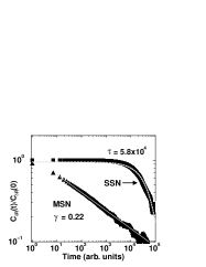
Figure 3: Auto-correlation functions of the resistance fluctuations calculated for a MSN (black triangles) and for a SSN (black squares). Both functions are obtained at 300 K. The solid and short dashed grey lines show the best-fit respectively with a power-law of exponent $\gamma=0.22$ and with an exponential with correlation time $\tau=5.8\times 10^{4}$. The time is expressed in iterative steps.

Figure 3 displays the auto-correlation functions of the resistance fluctuations in Figs. 1 and 2, corresponding to the MSN model (black triangles) and to the SSN model (black squares). A log-log representation is adopted for convenience. The solid and short dashed lines represent the best-fits to the two auto-correlation functions carried out, respectively, with a power-law and an exponential law. The fitting procedure confirms the exponential decay of the correlations in the resistance fluctuations of the SSN. Furthermore, it points out the existence of long-term correlations in the resistance fluctuations of the MSN, characterized by a power-law decay of the auto-correlation function:

$$C_{\delta R}(t)\sim t^{-\gamma}$$ (6)

with $0<\gamma<1$. In particular, here we have found a value $\gamma=0.22\pm 0.01$ for the correlation exponent. We stress that the above expression for the auto-correlation function implies a divergence of the correlation time, as can be easily seen by considering the following general definition of the correlation time bunde_pa2003 :

$$\tau=\int_{0}^{\infty}{C_{\delta R}(t)\over C_{\delta R}(0)}dt$$ (7)

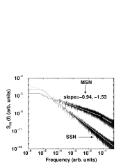
Figure 4: Power spectral density of the resistance fluctuations at 300 K calculated for a MSN (solid line) and for a SSN (dotted line). The grey solid line shows the best-fit to the MSN spectrum with a power-law of slope -0.94. The grey dashed curve represents the best-fit with a Lorentzian to the SSN spectrum.

Figure 4 shows the power spectral densities of the resistance fluctuations of a MSN and of a SSN calculated at 300 K by Fourier trasforming the auto-correlations functions of Fig. 3. Here, the two grey solid lines represent the best-fits with a power-law of the MSN spectrum in the low and high frequency regions. We can see that the resistance fluctuations of the multi-species network exhibit at low frequencies a power spectral density scaling as $1/f^{\alpha}$, with a value $\alpha=0.94$. We notice that this scaling behavior holds over several decades of frequency. This result is a consequence of the envelope of the different time scales associated with the different resistor species, described by Eq. (5). Instead, in the high frequency region, the slope of the spectrum is -1.53 (in fact, the slow relaxations are ineffective at such high frequencies). For contrast, the grey dashed curve in Fig. 4 is the best-fit with a Lorentzian to the SSN spectrum. The corner frequency of the Lorentzian, $f_{c}=4.0\times 10^{-6}$ (arbitrary units), is consistent with the correlation time reported in Fig. 3 and obtained by the best-fit of the corresponding auto-correlation function.

Now, we will discuss how the temperature of the thermal bath affects the resistance fluctuations of a multi-species network at equilibrium or nearly equilibrium conditions (low biases). In other terms, we will analyse the properties of the fluctuations in the Ohmic regime and for different temperatures. Figure 5 reports the resistance evolutions calculated at increasing temperatures: $T=400$ K (lower curve) and $T=600$ K (upper curve). Already this qualitative comparison between the $R(t)$ signals shows that a temperature increase implies a significant growth of both the average resistance and the variance of the resistance fluctuations (see also Figs. 1). Furthermore, this comparison points out a drastic reduction of the relaxation time at increasing temperatures (more than one order of magnitude when $T$ rises from 300 K to 400 K).

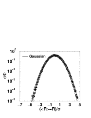
Figure 7: Normalized probability densities of the defect fraction fluctuations calculated at 300 K (full diamonds), 400 K (open circles), 500 K (open up-triangles), 600 K (full down-triangles) and 700 K (stars). Here $\sigma$ is the root-mean-square deviation from the average value of the defect fraction. The solid black curve is the Gaussian distribution.

The temperature is also found to affect the distribution of the resistance fluctuations by increasing its skewness, as shown in Fig. 6, which reports the probability density function (PDF) of the resistance fluctuations for several temperatures. A normalized lin-log representation has been adopted here for convenience ($\sigma$ is the root mean square deviation from the average resistance). The normalized Gaussian distribution is also reported for comparison. The figure shows a significant non-Gaussianity of the resistance fluctuations, which becomes stronger at high temperatures, when the system approaches failure conditions. This behavior is completely different from the behavior of the defect fraction fluctuations, shown in Fig. 7, which remains Gaussian at all temperatures. This different behavior can be easily understood. Actually, at increasing temperature, the local resistivity fluctuations become progressively larger. This fact emphasizes the dynamical redistribution of currents and brings to the emergence of long-range correlations inside the network seidler96 . Then, the violation of the validity conditions of the central limit theorem leads to a non-Gaussian resistance noise review ; kogan ; weissman_1f ; seidler96 ; ausloos . In other terms, the results in Fig. 6 imply that the correlation length of the resistance fluctuations progressively increases with the temperature. A discussion of the distribution of the resistance fluctuations and the role played on the non-Gaussianity by the size, shape and disorder of a SSN is reported in Refs. pen_ng, ; pen_ng_fn04, , where the link with the universal distribution of the fluctuations of Bramwell, Holdsworth and Pinton (BHP) bramwell ; clusel is analyzed.

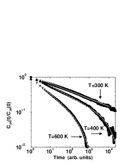
Figure 8: Auto-correlation functions of the resistance fluctuations of a MSN calculated at different temperatures. The solid grey curve shows the best-fit with a power-law to the auto-correlation function at 300 K (the same of Fig. 3). The dashed grey curves display the best-fit to the auto-correlation functions at 400 and 600 K with the function: $C(t)=C_{0}t^{-h}\exp[-t/u]$ (see the text for the values of the fit parameters). The time is expressed in iterative steps.

Figure 8 reports the auto-correlation functions of the resistance fluctuations of a MSN calculated at $400$ K and $600$ K. To help the comparison, the auto-correlation function at $300$ K (already shown in Fig. 3) has been drawn again in Fig. 8, together with its power-law best-fit (grey solid line). The dashed grey curves represent the best-fit to the correlation functions at $400$ K and $600$ K with the expression:

$$C_{\delta R}(t)=C_{0}t^{-h}\exp(-t/u)$$ (8)

The values of the best-fit parameters are: $C_{0}=1.13$, $h=0.30$ and $u=1.42\times 10^{4}$ for $T=400$ K and $C^{\prime}_{0}=0.965$, $h^{\prime}=0.46$ and $u^{\prime}=5.57\times 10^{2}$ for $T=600$ K. The fit to $C_{\delta R}$ with Eq. (8) is found to be very satisfactory. We conclude that at $T>300$ K, the auto-correlation function of the resistance fluctuations of the MSN is well described by a power-law with an exponential cut-off. Such kinds of mixed decays of the correlations, non-exponential and non power-law, are often found in the transition of a complex system from short-term correlated to long-term correlated regimes sornette ; weissman93 ; franz03 ; franz06 ; pen_epj ; caccioli ; coniglio ; parisi . It should be noted that for $u\rightarrow\infty$, Eq. (8) becomes a power-law, while for $h\rightarrow 0$, it describes an exponential decay. Actually, Fig. 8 highlights a strong reduction of the correlation time of the resistance fluctuations as the temperature increases. This result can be understood in terms of Eq. (4), by considering the thermally activated expressions of the breaking and recovery probabilities. Indeed, the increase of temperature above $T_{ref}$ implies the reduction of the ratio $\tau_{min}/\tau_{max}$ and the correspondent narrowing of the interval $[\tau_{min},\tau_{max}]$, where the $\tau_{i}$ are distributed. This trend tends to suppress the power-law decay of correlations in favor of the exponential decay. For similar reasons, the temperature decrease below $T_{ref}$, implies the opposite trend with the correlations keeping their power-law decay over wider time scales. For example, at $T=200$ K the ratio $\tau_{min}/\tau_{max}$ becomes $7.5\times 10^{7}$. Thus, we can define the transition temperature, $T^{*}$, as the temperature value which signs the crossing from a long-term correlated behavior (occurring for $T<T^{*}$), to a behavior characterized by a finite and relatively short correlation time (occurring for $T>T^{*}$).

The correlation time of the resistance fluctuations can be directly estimated by making use of Eq. (7) and Eq. (8). In terms of the best-fit parameters of the auto-correlation function, it is easy to derive the following analytical expression for $\tau$:

$$\tau=u^{1-h}\Gamma(1-h)$$ (9)

where $\Gamma$ is the Gamma function. The values of $\tau$ calculated in this way increase at decreasing temperatures. In particular, $\tau$ exhibits a sharp increase when $T$ approaches $T^{*}$, in agreement with the long-term decay of the correlation function at this temperature. We have found that the behavior of $\tau$ versus temperature is well fitted by the power-law: $\tau\sim(T-T^{*})^{-\theta}$. Then, the fit procedure allows us to determine the value of the transition temperature. We have found: $T^{*}=306$ K and $\theta=2.7$. Figure 9 reports the values of $\tau$ as a function of the difference $T-T^{*}$. The dashed straight line corresponds to the above mentioned power-law. Therefore, we can conclude that: $T^{*}\approx\Delta E^{*}/k_{B}$. Furthermore, as a result of the particular choice of the parameters adopted in the present calculations, the transition temperature is close also to the reference temperature, $T^{*}\approx T_{ref}$. However we remark that the temperature $T_{ref}$ has been introduced in the model merely to help the choice of the activation energies (to provide a sufficiently wide interval $[\tau_{min},\tau_{max}]$). While, $\Delta E^{*}$ is the relevant input parameter which determines $T^{*}$.

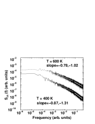
Figure 10: Power spectral density of the resistance fluctuations of a MSN at $T=400$ K and $T=600$ K. The grey lines show the best-fit with power-laws of slopes -0.87 and -0.78, respectively. The spectral density at 600 K has been multiplied by a factor 10 for visual reasons.

Figure 10 displays the spectral densities of the resistance fluctuations calculated at $400$ K and $600$ K. The grey lines represent the best-fits with a power-law of the MSN spectra in the low and high frequency regions. Precisely, at low-frequencies, the slopes of the lines are -0.87 and -0.78 respectively for $T=400$ K and $T=600$ K. Instead, at high frequencies the respective slopes are -1.31 and -1.02. Thus, in both frequency regions, low and high, the slopes of the specra are reduced when the temperature increases. We conclude that at $T>T^{*}$ the power spectrum keeps the $1/f^{\alpha}$ form with the value of ${\alpha}$ significantly decreasing below unity. This decrease is pointed out in Fig. 11, which reports ${\alpha}$ as a function of the temperature. The dashed line in Fig. 11 is the best-fit with a linear law. We notice that such a decrease of the exponent, from $\alpha\approx 1$ to $\alpha\approx 0.8-0.5$, is frequently observed in the experiments at intermediate temperatures review ; kogan ; upon05 ; bosman ; alers . On the other hand, many experiments have pointed out a strong dependence of the detailed behavior of $\alpha(T)$ also on the particular material review ; kogan ; upon05 ; alers . In this respect, we remark that in this work we are focusing our attention to the general features of the spectra, related to the term of correlations, rather than to the interpretation of a particular set of experiments. Actually, in our model the quantity $\Delta E^{*}$ (determining the transition temperature $T^{*}$) is the input parameter which can be adjusted for a quantitative fit of experiments. Furthermore, we stress that the monotonic decrease of ${\alpha}$ for $T>T^{*}$ is obtained here in the linear regime of currents, i.e. neglecting Joule heating effects. Actually, these effects, whose importance also depends on the temperature, can give rise to a more complicated behavior of ${\alpha}$ versus $T$, which are outside the interest of this research but can be implemented with minor efforts.

Now, to complete the analysis of the MSN model, we consider the dependence on the temperature of the average resistance, $\langle R\rangle$, and of the variance of the resistance fluctuations, $\langle(\Delta R)^{2}\rangle$ for a multi-species network in nearly equilibrium conditions. This dependence has been already qualitatively depicted in Figs. 1 and 5. However here we want to quantify these behaviors, also with the purpose of checking by numerical results the validity of the mean field-like approach discussed in Section II. Figure 12 displays $\langle R\rangle$ as a function of the temperature, while the inset shows the dependence on the temperature of the average defect fraction. We have performed a one parameter best-fit of the numerical values of $\langle p\rangle$ with the expression: $\langle p\rangle=c_{p}/(1+e^{\Delta E^{*}/K_{B}T})$. We have found $c_{p}=0.93\pm 0.03$, a value compatible with the expression: $\langle p\rangle\approx 1/(1+e^{\Delta E^{*}/K_{B}T})$. Thus, Eq. (2) qualitatively accounts for the behavior of the average defect fraction versus temperature.

For what concerns the dependence on temperature of the average resistance, in percolation theory stauffer it is well known the following scaling relation between the network resistance and the defect fraction: $R\sim|p-p_{c}|^{-\mu}$. We note that in the present model at the vanishing current limit prl_stat , the percolation is uncorrelated and the exponent $\mu$ takes the universal value stauffer $\mu=1.303$, while $p_{c}=0.5$ percol ; stauffer . The dashed curve in Fig. 12 shows the best-fit of the numerical data for the average resistance with the expression: $\langle R\rangle=c_{R}|\langle p\rangle-p_{c}|^{-\mu}$. In the best-fit procedure the values of $\mu$ and $p_{c}$ have been taken fixed to their theoretical values, while we have taken: $\langle p\rangle=c_{p}/(1+e^{\Delta E^{*}/K_{B}T})$. The values found for the fitting parameters are: $c_{R}=0.42\pm 0.01$ $\Omega$ and $c_{p}=0.80\pm 0.03$. Thus, the dependence on temperature of the average resistance of a MSN in the linear regime is well described by the usual scaling relation coupled with the mean field-like expression of $\langle p\rangle$.

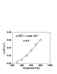
Figure 13: Variance of the resistance fluctuations as function of the temperature. The variance is espressed in $\Omega^{2}$ and the temperature in K. The dashed straight line shows a best-fit with the expression reported in the figure (see the text for the values of fit parameters).

Figure 13 reports the variance of the resistance fluctuations as a function of the temperature. This behavior can be easily understood by considering before the power-law relation between the variance of the resistance fluctuations and the average resistance stauffer ; rammal85 : $\langle(\Delta R)^{2}\rangle\sim\langle R\rangle^{\eta}$, often written in terms of the relative variance, as:

$$\langle(\Delta R)^{2}\rangle/\langle R\rangle^{2}\ \sim\langle R\rangle^{s}$$ (10)

where $s=\eta-2$. By reporting on a log-log plot the relative variance $\langle(\Delta R)^{2}\rangle/\langle R\rangle^{2}$ versus $\langle R\rangle$, the calculated slope provides for the exponent $s$ the value $s=2.6\pm 0.01$ We note that this value of the relative noise exponent agrees with the value reported in Ref. prl_stat, . This agreement is consistent with the fact that the MSN model generalizes the results of Ref. prl_stat, to networks characterized by $1/f^{\alpha}$ noise. Now, we can use the information on the exponent $\eta=s+2=4.6$ to check the consistency among the dependence on temperature of $\langle(\Delta R)^{2}\rangle$, Eq. (2), the scaling relations between $\langle R\rangle\sim\langle p\rangle$ and between $\langle(\Delta R)^{2}\rangle\sim\langle R\rangle$. The solid curve in Fig. 13 shows the best-fit to the variance of the resistance fluctuations considered versus temperature, with the following expression: $\langle(\Delta R)^{2}\rangle=c_{\Delta}c_{R}^{\eta}|\langle p\rangle-p_{c}|^{-\mu\eta}$ where the fitting parameters take the values: $c_{\Delta}=(4.42\pm 0.04)\times 10^{6}$, $c_{R}=1.0\pm 0.04$ and $c_{p}=0.74\pm 0.03$. Thus, a mean field-like framework is overall able to account for the dependence on temperature of the lowest two moments of resistance fluctuation distribution.

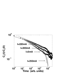
Figure 15: Auto-correlation functions of the resistance fluctuations of a MSN at room temperature for increasing value of the external current. Ohmic regime: $I=5$ mA (open square), non-linear-regime: $I=200$ mA (black triangles), $I=220$ mA (open circles) and $I=250$ mA (grey diamonds). The dotted grey line is the best-fit with a power-law, the dashed lines are the best-fit with the function: $C(t)=C_{0}t^{-h}\exp[-t/u]$ (see the text for the values of the fit parameters).

Until now we have analysed the resistance fluctuations of the network in equilibrium or in nearly equilibrium conditions, in the Ohmic regime, and for different temperatures. Now, we will briefly discuss the non equilibrium properties of the fluctuations at high biases, in the nonlinear regime, and for a given temperature. Figure 15 shows the auto-correlation functions of the resistance fluctuations of a MSN for increasing values of the external current. All the functions are calculated at $300$ K. The open squares represent the auto-correlation of the resistance fluctuations in the Ohmic regime: $I=5$ mA, the other three curves correspond to the non-linear regime. Precisely, black triangles: $I=200$ mA; open circles: $I=220$ mA; grey diamonds: $I=250$ mA $>I_{B}$. Thus, the last curve corresponds to failure of the network, i.e. non-stationary resistance fluctuations. In this case, the auto-correlation function has been calculated by considering only the nearly-stationary portion of the $R(t)$ signal (after subtraction of a linear trend). The dotted grey line is the best-fit with a power-law of slope $-0.22\pm 0.01$, the dashed lines are the best-fits with Eq. (8). The values of the parameter $h$ corresponding respectively to: $I=200$, $220$, $250$ mA are the following: $h=0.19$, $0.17$, $0.11$ (in all cases, the numerical error is estimated as $\pm 0.01$). The values of the parameter $u$ corresponding to the same currents respectively are: $(1.26\pm 0.01)\times 10^{5}$, $(9.15\pm 0.01)\times 10^{4}$, $(5.84\pm 0.01)\times 10^{3}$. Thus, both $h$ and $u$ decrease at increasing biases and for high biases $h\rightarrow 0$. In other terms, at increasing currents, time correlations decay progressively faster, the long-term correlated behavior is destroyed and it emerges a trend towards a simple exponential decay.

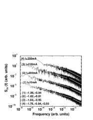
Figure 16: Power spectral density of the resistance fluctuations of a MSN at room temperature for increasing value of the external current. Ohmic regime: curve (1) $I=5$ mA; non-linear-regime: curve (2) $I=200$ mA, curve (3) $I=220$ mA and curve (4) $I=250$ mA. The solid grey lines are the best-fit with power-laws, the resulting slopes in the different regions of the spectrum are reported in the figure. For visual reasons curve (2) has been multiplied by a factor $2\times 10^{2}$, curve (3) by a factor $2\times 10^{4}$ and curve (4) by $1\times 10^{6}$.

The corresponding effect in the frequency domain of increasing biases is shown in Fig. 16, which reports the power spectral densities at $300$ K. The curve (1) is obtained for the Ohmic regime ($I=5$ mA); the other three curves display the spectra in the non-linear regime. The solid grey lines are the best-fits with power-laws in the low and high frequency regions of the spectrum. The slopes are specified in the figure. We note that: i) the corner frequency between the two regions progressively moves towards lower frequencies at increasing biases; ii) the slopes in the high frequency region are: $-1.56$, $-1.62$, $-1.66$, $-1.78$ respectively for $I=5$, $200$, $220$ and $250$ mA, i.e. the slopes increase at increasing currents (in all cases, the numerical error on the slope values is estimated as $\pm 0.01$). Thus, at high biases, the spectral densities show a trend towards a transition from an $1/f$ to a Lorentzian behavior. However, we remark that for the present choice of the initial conditions and/or the numerical values of the parameters used in these calculations we have not got a pure Lorentzian spectrum.

IV Conclusions

We have developed a stochastic model to investigate the $1/f^{\alpha}$, with $0<\alpha<2$, resistance noise in disordered materials. More precisely, we have considered the resistance fluctuations of a thin resistor with granular structure in different stationary states: from nearly equilibrium up to far from equilibrium conditions. Furthermore we have also considered fluctuations in non-stationary states, associated with failure of the electric properties. This system has been modeled as a two-dimensional network made by different species of elementary resistors. The steady state of this multi-species network is determined by the competition among different thermally activated and stochastic processes of breaking and recovery of the elementary resistors. The network properties have been studied by Monte Carlo simulations as a function of the temperature and applied current, in both Ohmic and non-Ohmic regimes. A mean field-like framework has been also used to qualitatively describe the dependence on temperature of the lowest two moments of the resistance fluctuation distribution. Furthermore, the correlation properties of the resistance fluctuations have been analyzed in both the time and the frequency domains. The model gives rise to resistance fluctuations with different power spectra, depending on the external conditions. Thus it provides a unified approach to the study of materials exhibiting either Lorentzian noise or $1/f^{\alpha}$ noise. By analyzing the correlations in the time domain, it has been found that the resistance fluctuations display a cross-over from long-term correlations to intermediate-term correlations. Although a trend towards an exponential decay has been identified, for the present choice of the parameters/initial conditions, we have not got a single exponential decay. However, the model proposed seems able to account for the complex interplay exerted on the correlation properties of the resistance fluctuations by the external conditions and resulting in the complicate behavior of the noise exponent observed in many experiments. In perspective, it should be explored the role of different initial conditions: such as unequal presence of the species and/or non-uniform distribution inside the network, which can give rise to interesting spatio-temporal organization patterns.

Figure 1: Resistance evolution of a multi-species network (MSN model) calculated at 300 K. The resistance is espressed in Ohm and the time in iterative steps. The inset highlights the resistance fluctuations on an enlarged time scale. In particular, the time units are divided by a factor $10^{-5}$.

Figure 2: Resistance evolution of a single-species network (SSN model) calculated at 300 K. The resistance is espressed in Ohm and the time in iterative steps. The inset displays the resistance fluctuations on the same enlarged time scale of the inset in Fig. 1. (the vertical scales of the insets in the two figures are different).

Figure 5: Resistance evolution of a MSN at 400 K and 600 K. The resistance is espressed in Ohm and the time in iterative steps.

Figure 6: Normalized probability densities of the resistance fluctuations of a MSN calculated at 300 K (full diamonds), 400 K (open circles), 500 K (open up-triangles), 600 K (full down-triangles) and 700 K (stars). $\sigma$ is the root-mean-square deviation from the average resistance. The solid black curve is the Gaussian distribution and the dashed one the BHP distribution (see text).

Figure 9: Correlation time of the resistance fluctuations of a MSN as a function of the difference $T-T^{*}$. The time is expressed in iterative steps and the temperature in K. The value of $T^{*}$ is reported in the figure. The dashed line shows the fit with a power-law of exponent $\theta=2.7$.

Figure 11: Noise exponent $\alpha$ as function of the temperature. The dashed line refers to a linear best-fit of the calculated values of the exponent.

Figure 12: Variation of the average resistance (full circles) and average defect fraction (stars, in the inset) as function of the temperature. The resistance is espressed in Ohm and the temperature in K. The solid and dashed straight lines are the best-fits with the expressions reported in the figure (see the text for the values of fit parameters).

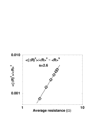
Figure 14: Relative variance of the resistance fluctuations as a function of the average resistance (this last expressed in Ohm). The dashed line shows a best-fit with a power-law of exponent $s=2.6$.

References

- (1) M. B. Weissman, Rev. Mod. Phys., 60, 537, (1988); F. N. Hooge, T. G. M. Kleinpenning and L. K. J. Vandamme, Rep. Prog. Phys., 44, 479 (1981); P. Dutta and P. M. Horn, Rev. Mod. Phys., 53, 497 (1981).
- (2) Sh. Kogan, Electronic Noise and Fluctuations in Solids, Cambridge Univ. Press, Cambridge (1996).
- (3) Unsolved Problems of Noise and Fluctuations, ed. by L. Reggiani, C. Pennetta, V. Akimov, E. Alfinito and M. Rosini, AIP Conf. Proc. 800, New York (2005); Noise and Fluctuations, ed. by T. González, J. Mateos and D. Pardo, AIP Conf. Proc. 780, New York (2005).
- (4) S. Reza, Q. T. Huynh, G. Bosman, J. Sippel-Oakley and A. G. Rinzler, J. Appl. Phys., 99, 114309 (2006); S. Reza, G. Bosman, M. S. Islam, T. I. Kamins, IEEE Trans. on Nanotech., 5, 523 (2006).
- (5) A. Bid, A. Bora, A. K. Raychaudhuri, Nanotechnology, 17, 152 (2006).
- (6) S. Soliveres, J. Gyani, C. Delseny, A. Hoffmann and F. Pascal, J. Appl. Phys., 90, 082107 (2007).
- (7) M. Tarsov, J. Svensson, L. Kuzmin, E. E. B. Campbell, J. Appl. Phys., 90, 163503 (2007).
- (8) J. Tersoff, Nanoletters, 7, 194 (2007).
- (9) Y.M. Lin, J. Appenzeller, J. Knoch, Z. Chen and P. Avouris, Nanoletters, 6, 930 (2006).
- (10) G. Deville, R. Leturcq, D. L’Hôte, R. Tourbot, C. J. Mellor and M. Henini, Physica E, 34, 252 (2006); R. Leturcq, D. L’Hôte, R. Tourbot, C. J. Mellor and M. Henini, Phys. Rev. Lett., 90, 076402 (2003).
- (11) S. Torquato, Random Heterogeneous Materials, Microscopic and Macroscopic Properties, Springer-Verlag, New York, 2002.
- (12) M. Sahimi, Phys. Rep. 306, 213 (1998).
- (13) C. D. Mukherjee and K. K. Bardhan, Phys. Rev. Lett. 91, 025702 (2003); C. D. Mukherjee, K. K. Bardhan and M. B. Heaney, Phys. Rev. Lett. 83, 1215 (1999); U. N. Nandi, C. D. Mukherjee and K. K. Bardhan, Phys. Rev. B, 54, 12903 (1996).
- (14) K. M. Abkemeier and D. G. Grier, Phys. Rev. B, 54, 2723 (1996).
- (15) I. Bloom and I. Balberg, Appl. Phys. Lett., 74, 1427 (1999).
- (16) L. M. Lust and J. Kakalios, Phys. Rev. Lett., 75, 2192 (1995).
- (17) L.M. Lust and J. Kakalios, Phys. Rev. E, 50, 3431 (1994).
- (18) G. B. Alers, M. B. Weissman, R. S. Averback and H. Shyu, Phys. Rev. B, 40, 900 (1989).
- (19) G. Snyder, M. B. Weissman, H. T. Hardner and C. Parman, Phys. Rev. B, 56, 9205 (1997).
- (20) J. Planes and A. Francois, Phys. Rev. B, 70, 184203 (2004).
- (21) A. Carbone, B. K. Kotowska and D. Kotowski, Phys. Rev. Let., 95, 236601 (2005).
- (22) K. M. Chen, G. W. Huang, D. Y. Chiu, H. J. Huang and C. Y. Chang, Appl. Phys. Lett., 81, 2578 (2002).
- (23) S. Kar, A. K. Raychaudhuri, A. Ghosh, H. V. Löhneysen and G. Weiss, Phys. Rev. Lett., 91, 216603 (2003).
- (24) C. Chiteme, D. S. McLachlan and I. Balberg, Phys. Rev. B, 67, 024207 (2003).
- (25) V. Emelianov, G. Ganesan, A. Puzic, S. Schulz, M. Eizenberg, H. U. Habermeier and H. Stoll, in Noise as a Tool for Studying Materials, p. 271, ed. by M. B. Weissman, N. E. Israeloff and A. S. Kogan, Procs. SPIE, 5112, Int. Soc. Opt. Eng., Bellingham (2004).
- (26) N. Garnier and S. Ciliberto, Phys. Rev. E, 71, 060101 (2005).
- (27) J. V. Andersen, D. Sornette and K.T. Leung, Phys. Rev. Lett. 78, 2140 (1997); L. Lamaignère, F. Carmona and D. Sornette, Phys. Rev. Lett. 77, 2738 (1996).
- (28) T. Bodineau and B. Derrida, Phys. Rev. Lett., 92, 180601 (2004).
- (29) C. Pennetta, L. Reggiani, G. Trefán and E. Alfinito, Phys. Rev. E, 65, 066119 (2002); C. Pennetta, Fluctuation and Noise Letters, 2, R29 (2002).
- (30) C. Pennetta, E. Alfinito, L. Reggiani and S. Ruffo, Physica A, 340, 380, (2004); C. Pennetta, E. Alfinito, L. Reggiani and S. Ruffo, Semicond. Sci. Technol., 19, S164 (2004).
- (31) T. Antal, M. Droz, G. Györgyi and Z. Rácz, Phys. Rev. Lett., 87, 240601 (2001).
- (32) G. Györgyi, N. R. Moloney, K. Ozogány and Z. Rácz, Phys. Rev. E, 75, 021123 (2007).
- (33) P. Dutta, P. Dimon and P.M. Horne, Phys. Rev. Lett., 43, 646 (1979).
- (34) Y. C. Zhang and S. Liang, Phys. Rev. B, 36, 2345 (1987).
- (35) M. B. Weissman Rev. Mod. Phys., 65, 829 (1993).
- (36) P. Bak, C. Tang and K. Wiesenfeld, Phys. Rev. Lett., 59, 381 (1987); P. De Los Rios and Y. C. Zhang, Phys. Rev. Lett., 82, 472 (1999).
- (37) L. Laurson, M. J. Alava and S. Zapperi, J. of Stat. Mec. 2005, 8 (2005).
- (38) J. Wang, S. Kadar, P. Jung and K. Showalter, Phys. Rev. Lett., 82, 855 (1999); S. S. Manna and D. V. Khakhar, Phys. Rev. E, 58, R6935 (1998).
- (39) B. Kaulakys and J. Ruseckas, Phys. Rev. E, 70, 020101 (2004).
- (40) L. B. Kiss and P. Svedlindh, Phys. Rev. Lett., 71, 2817 (1993).
- (41) M. Celasco and R. Eggenhöffner, Eur. Phys. J. B, 23, 415 (2001).
- (42) A. L. Rakhmanov, K.I. Kugel, Y.M. Blanter and M.Y. Kagan, Phys. Rev.B, 63, 174424 (2001).
- (43) B. I. Shklovskii, Phys. Rev. B, 67, 045201 (2003).
- (44) K. Shtengel and C. C. Yu, Phys. Rev. B, 67, 165106 (2004).
- (45) J. Davidsen, H. G. Schuster, Phys. Rev. E, 65, 026120 (2002).
- (46) D. Stauffer and A. Aharony, Introduction to Percolation Theory, Taylor & Francis, London (1992).
- (47) G. Odor, Rev. of Mod. Phys. 76, 663 (2004).
- (48) L. de Arcangelis, S. Redner and A. Coniglio, Phys. Rev. B, 34, 4656 (1986).
- (49) R. Rammal, C. Tannous and A. M. S. Tremblay, Phys. Rev. A, 31, 2662 (1985) and R. Rammal, C. Tannous, P. Breton and A. M. S. Tremblay, Phys. Rev. Lett., 54, 1718 (1985).
- (50) Y. Park, A.B. Harris and T.C. Lubensky, Phys. Rev. B, 35, 5048 (1987).
- (51) D. J. Bergman, Phys. Rev. B, 39, 4598 (1989).
- (52) R.R. Tremblay, G. Albinet and A. M. S. Tremblay, Phys. Rev. B, 43, 11546 (1991).
- (53) Z. Gingl, C. Pennetta, L. B. Kiss, and L. Reggiani, Semic. Sci. Technol., 11, 1770 (1996).
- (54) G.T. Seidler, S.A. Solin and A.C. Marley, Phys. Rev. Lett., 17, 3049 (1996).
- (55) D. Sornette, Critical Phenomena in Natural Sciences, Chaos, Fractals, Selforganization and Disorder: Concepts and Tools, Springer, Berlin, (2004).
- (56) C. Pennetta, L. Reggiani and G. Trefán, Phys. Rev. Lett., 84, 5006 (2000).
- (57) C. Pennetta, G. Trefan and L. Reggiani, Phys. Rev. Lett., 85, 5238 (2000).
- (58) C. Pennetta, E. Alfinito, L. Reggiani, F. Fantini, I. De Munari and A. Scorzoni, Phys. Rev. B, 70, 174305 (2004).
- (59) C. Pennetta, E. Alfinito, L. Reggiani and S. Ruffo, in Noise in Complex Systems and Stochastic Dynamics II, p. 38, ed. by Z. Gingl and J. M. Sancho and L. Schimansky-Geier and J. Kertesz, Procs. SPIE, 5471, Int. Soc. Opt. Eng., Bellingham (2004).
- (60) Actually, two-dimensional resistor networks of sizes with , or networks with different lattice structures can be easily considered.
- (61) D. Sornette and C. Vanneste, Phys. Rev. Lett., 68, 612, (1992); C. Vanneste and D. Sornette, J. Phys. I (France), 2, 16212, (1992).
- (62) for bond percolation on a square-lattice network of size in the limit . See for example Ref. stauffer, .
- (63) We take the correlation time associated with the fluctuations of the defect fraction, comparable with that corresponding to the fluctuations of the resistance, , i.e. we take . Our simulations confirm this assumption.
- (64) A. Bunde, J. F. Eichner, S. Havlin and J. W. Kantelhardt, Physica A, 330, 1 (2003).
- (65) N. Vandewalle, M. Ausloos, M. Houssa, P. W. Mertens, M. M. Heyns, Appl. Phys. Let., 74, 1579 (1999).
- (66) S. T. Bramwell, P. C. W. Holdsworth and J. F. Pinton, Nature, 396, 552 (1998) and S. T. Bramwell, K.Christensen, J. Y. Fortin, P. C. W. Holdsworth, H. J. Jensen, S. Lise, J. M. López, M. Nicodemi, J. F. Pinton and M. Sellitto, Phys. Rev. Lett., 84, 3744 (2000).
- (67) M. Clusel, J. Y. Fortin and P. C. W. Holdsworth, Phys. Rev. E, 70, 046112 (2004).
- (68) S. Franz, V. Lecomte and R. Mulet, Phys. Rev. E, 68, 066128 (2003).
- (69) S. Franz, Europhys. Lett., 73, 492 (2006).
- (70) C. Pennetta, Eur. Phys. J. B, 50, 95 (2006).
- (71) F. Caccioli, S. Franz and M. Marsili, J. Stat. Mech., P07006 (2008).
- (72) T. Abete, A. de Candia, E. Del Gado, A. Fierro and A. Coniglio, Phys. Rev. Let., 98, 088301 (2007).
- (73) G. Parisi and F. Zamponi, arXiv:0802.2180 (2008).